Inf 2B: Graphs, BFS, DFS

Kyriakos Kalorkoti

School of Informatics

University of Edinburgh

1 / 26

Directed and Undirected Graphs

I A graph is a mathematical structure consisting of a set of

vertices and a set of edges connecting the vertices.

I Formally: G = (V ,E), where V is a set and E ✓ V ⇥ V .

I For edge e = (u, v) we say that e is directed from u to v .

I G = (V ,E) undirected if for all v ,w 2 V :

(v ,w) 2 E () (w , v) 2 E .

Otherwise directed.

Directed ⇠ arrows (one-way)

Undirected ⇠ lines (two-way)

I We assume V is finite, hence E is also finite.

2 / 26

A directed graph

G = (V ,E),

V =�

0, 1, 2, 3, 4, 5, 6 ,

E =�(0, 2), (0, 4), (0, 5), (1, 0), (2, 1), (2, 5),

(3, 1), (3, 6), (4, 0), (4, 5), (6, 3), (6, 5) .

0

2 3

654

1

3 / 26

An undirected graph

ba

d

e

f

g

c

4 / 26

Examples

I Road Maps.Edges represent streets and vertices represent crossings

(junctions).

I Computer Networks.

Vertices represent computers and edges represent

network connections (cables) between them.

I The World Wide Web.

Vertices represent webpages, and edges represent

hyperlinks.

I . . .

5 / 26

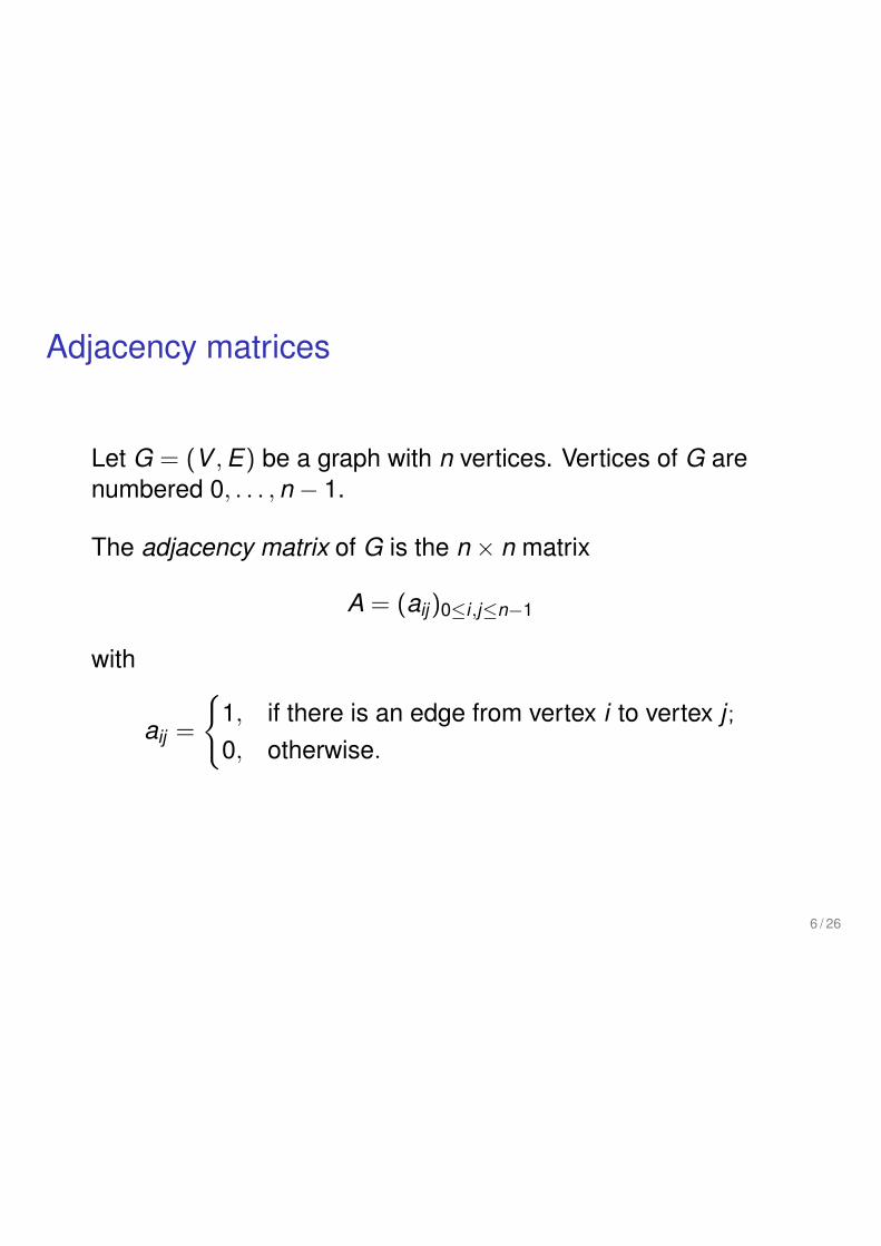
Adjacency matrices

Let G = (V ,E) be a graph with n vertices. Vertices of G are

numbered 0, . . . , n � 1.

The adjacency matrix of G is the n ⇥ n matrix

A = (aij)0i,jn�1

with

aij =

(1, if there is an edge from vertex i to vertex j ;0, otherwise.

6 / 26

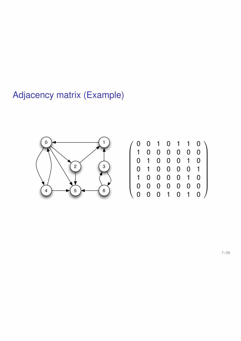
Adjacency matrix (Example)

0

2 3

654

10

BBBBBBBB@

0 0 1 0 1 1 0

1 0 0 0 0 0 0

0 1 0 0 0 1 0

0 1 0 0 0 0 1

1 0 0 0 0 1 0

0 0 0 0 0 0 0

0 0 0 1 0 1 0

1

CCCCCCCCA

7 / 26

Adjacency lists

Array with one entry for each vertex v , which is a list of all

vertices adjacent to v .

Example

0

2 3

654

12 4

5

5

1

0

35

50

61

0

1

2

5

6

3

4

8 / 26

Quick Question

Given: graph G = (V ,E), with n = |V |, m = |E |.For v 2 V , we write in(v) for in-degree, out(v) for out-degree.

Which data structure has faster (asymptotic) worst-case

running-time, for checking if w is adjacent to v , for a given pair

of vertices?

1. Adjacency list is faster.

2. Adjacency matrix is faster.

3. Both have the same asymptotic worst-case running-time.

4. It depends.

Answer: 2. For an Adjacency Matrix we can check in ⇥(1) time.

An adjacency list structure takes ⇥(1 + out(v)) time.

9 / 26

Quick Question

Given: graph G = (V ,E), with n = |V |, m = |E |.For v 2 V , we write in(v) for in-degree, out(v) for out-degree.

Which data structure has faster (asymptotic) worst-case

running-time, for visiting all vertices w adjacent to v , for a given

vertex v?

1. Adjacency list is faster.

2. Adjacency matrix is faster.

3. Both have the same asymptotic worst-case running-time.

4. It depends.

Answer: 3. Adjacency matrix requires ⇥(n) time always.

Adjacency list requires ⇥(1 + out(v)) time.

In worst-case out(v) = ⇥(n).

10 / 26

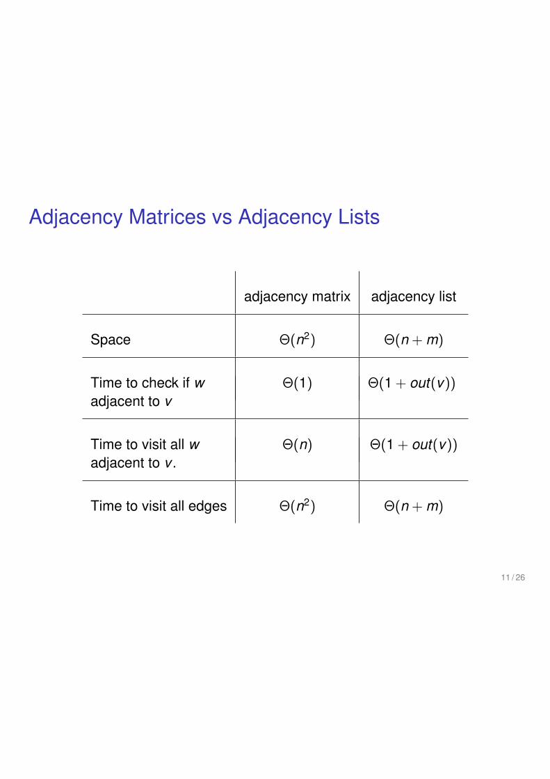
Adjacency Matrices vs Adjacency Lists

adjacency matrix adjacency list

Space ⇥(n2) ⇥(n + m)

Time to check if w ⇥(1) ⇥(1 + out(v))adjacent to v

Time to visit all w ⇥(n) ⇥(1 + out(v))adjacent to v .

Time to visit all edges ⇥(n2) ⇥(n + m)

11 / 26

Sparse and dense graphs

G = (V ,E) graph with n vertices and m edges

Observation: m n2

I G dense if m close to n2

I G sparse if m much smaller than n2

12 / 26

Graph traversals

A traversal is a strategy for visiting all vertices of a graph while

respecting edges.

BFS = breadth-first search

DFS = depth-first search

General strategy:

1. Let v be an arbitrary vertex

2. Visit all vertices reachable from v3. If there are vertices that have not been visited, let v be

such a vertex and go back to (2)

13 / 26

Graph Searching (general Strategy)

Algorithm searchFromVertex(G, v)

1. mark v2. put v onto schedule S3. while schedule S is not empty do

4. remove a vertex v from S5. for all w adjacent to v do

6. if w is not marked then

7. mark w8. put w onto schedule S

Algorithm search(G)

1. ensure that each vertex of G is not marked

2. initialise schedule S3. for all v 2 V do

4. if v is not marked then

5. searchFromVertex(G, v)14 / 26

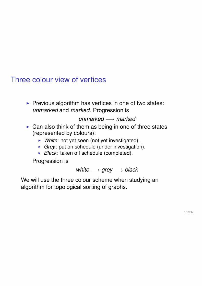
Three colour view of vertices

I Previous algorithm has vertices in one of two states:

unmarked and marked. Progression is

unmarked �! markedI Can also think of them as being in one of three states

(represented by colours):

I White: not yet seen (not yet investigated).

I Grey : put on schedule (under investigation).

I Black : taken off schedule (completed).

Progression is

white �! grey �! black

We will use the three colour scheme when studying an

algorithm for topological sorting of graphs.

15 / 26

BFS

Visit all vertices reachable from v in the following order:

I vI all neighbours of vI all neighbours of neighbours of v that have not been

visited yet

I all neighbours of neighbours of neighbours of v that have

not been visited yet

I etc.

16 / 26

BFS (using a Queue)

Algorithm bfs(G)

1. Initialise Boolean array visited , setting all entries to FALSE.

2. Initialise Queue Q3. for all v 2 V do

4. if visited [v ] = FALSE then

5. bfsFromVertex(G, v)

17 / 26

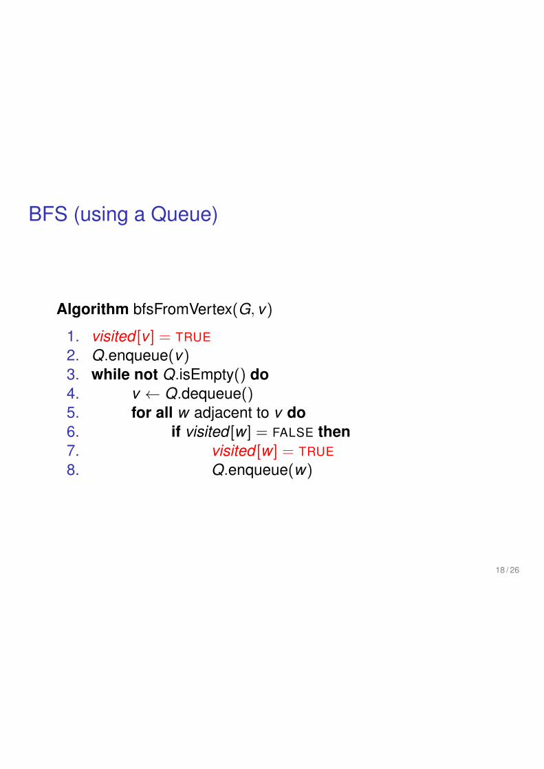
BFS (using a Queue)

Algorithm bfsFromVertex(G, v)

1. visited [v ] = TRUE

2. Q.enqueue(v)3. while not Q.isEmpty() do

4. v Q.dequeue()5. for all w adjacent to v do

6. if visited [w ] = FALSE then

7. visited [w ] = TRUE

8. Q.enqueue(w)

18 / 26

Algorithm bfsFromVertex(G, v)

1. visited [v ] = TRUE

2. Q.enqueue(v)3. while not Q.isEmpty() do

4. v Q.dequeue()5. for all w adjacent to v do

6. if visited [w ] = FALSE then

7. visited [w ] = TRUE

8. Q.enqueue(w)

0

2 3

654

1

19 / 26

Quick Question

Given a graph G = (V ,E) with n = |V |, m = |E |, what is the

worst-case running time of BFS, in terms of m, n?

1. ⇥(m + n)2. ⇥(n2)

3. ⇥(mn)4. Depends on the number of components.

Answer: 1. To see this need to be careful about bounding

running time for the loop at lines 5–8.

Must use the Adjacency List structure.

Answer: 2. if we use adjacency matrix representation.

20 / 26

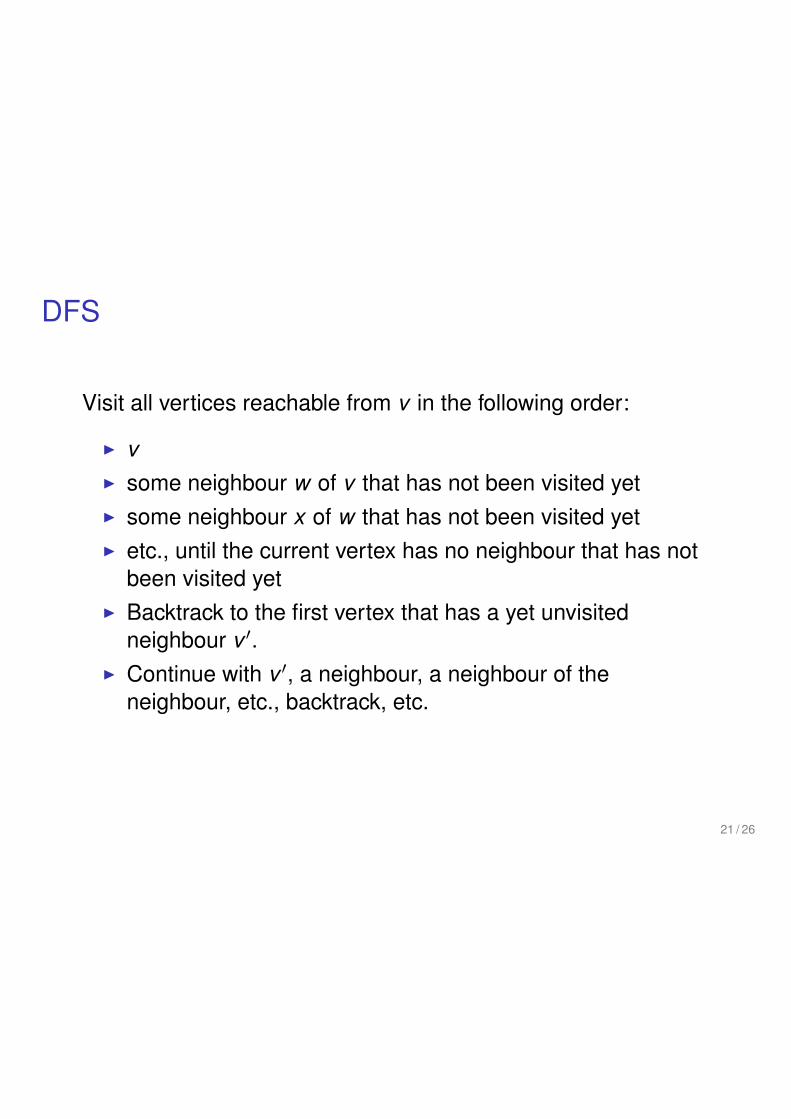
DFS

Visit all vertices reachable from v in the following order:

I vI some neighbour w of v that has not been visited yet

I some neighbour x of w that has not been visited yet

I etc., until the current vertex has no neighbour that has not

been visited yet

I Backtrack to the first vertex that has a yet unvisited

neighbour v 0.

I Continue with v 0, a neighbour, a neighbour of the

neighbour, etc., backtrack, etc.

21 / 26

DFS (using a stack)

Algorithm dfs(G)

1. Initialise Boolean array visited , setting all to FALSE

2. Initialise Stack S3. for all v 2 V do

4. if visited [v ] = FALSE then

5. dfsFromVertex(G, v)

22 / 26

DFS (using a stack)

Algorithm dfsFromVertex(G, v)

1. S.push(v)2. while not S.isEmpty() do

3. v S.pop()4. if visited [v ] = FALSE then

5. visited [v ] = TRUE

6. for all w adjacent to v do

7. S.push(w)

0

2 3

654

1

23 / 26

Recursive DFS

Algorithm dfs(G)

1. Initialise Boolean array visitedby setting all entries to FALSE

2. for all v 2 V do

3. if visited [v ] = FALSE then

4. dfsFromVertex(G, v)

Algorithm dfsFromVertex(G, v)

1. visited [v ] TRUE

2. for all w adjacent to v do

3. if visited [w ] = FALSE then

4. dfsFromVertex(G,w)

24 / 26

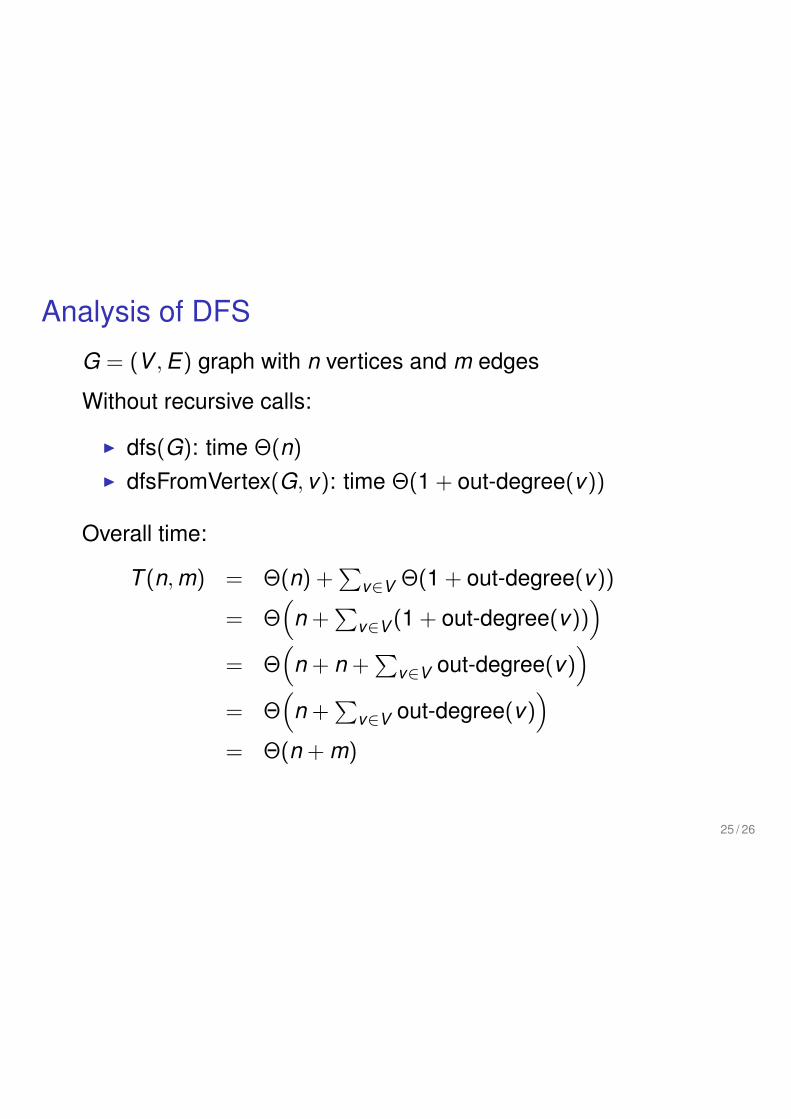
Analysis of DFS

G = (V ,E) graph with n vertices and m edges

Without recursive calls:

I dfs(G): time ⇥(n)I dfsFromVertex(G, v): time ⇥(1 + out-degree(v))

Overall time:

T (n,m) = ⇥(n) +P

v2V ⇥(1 + out-degree(v))

= ⇥⇣

n +P

v2V (1 + out-degree(v))⌘

= ⇥⇣

n + n +P

v2V out-degree(v)⌘

= ⇥⇣

n +P

v2V out-degree(v)⌘

= ⇥(n + m)

25 / 26