Genetic Theory

Manuel AR Ferreira

Egmond, 2007

Massachusetts General HospitalHarvard Medical School

Boston

Outline

1. Aim of this talk

2. Genetic concepts

3. Very basic statistical concepts

4. Biometrical model

1. Aim of this talk

Gene mapping

LOCALIZE and then IDENTIFY a locus that regulates a trait

Linkage analysis

Association analysis

If a locus regulates a trait, Trait Variance and Covariance between individuals can be expressed as a function of this locus.

Linkage:

Association:If a locus regulates a trait, Trait Mean in the population can be expressed as a function of this locus.

Revisit common genetic parameters - such as allele frequencies, genetic effects, dominance, variance components, etc

Use these parameters to construct a biometrical genetic model

Model that expresses the:

(1) Mean

(2) Variance

(3) Covariance between individuals

for a quantitative phenotype as a function of the genetic parameters of a given locus.

2. Genetic concepts

A. Population level

B. Transmission level

C. Phenotype level

G

G

G

G

G

G

G

G

G

GG

G

G

G

G

G

GG

G

G

G

G

GG

PP

Allele and genotype frequencies

Mendelian segregationGenetic relatedness

Biometrical modelAdditive and dominance components

A. Population

level 1. Allele frequencies

A single locus, with two alleles - Biallelic / diallelic - Single nucleotide polymorphism, SNP

Alleles A and a - Frequency of A is p - Frequency of a is q = 1 – p

A a

A a

Every individual inherits two alleles - A genotype is the combination of the two alleles - e.g. AA, aa (the homozygotes) or Aa (the heterozygote)

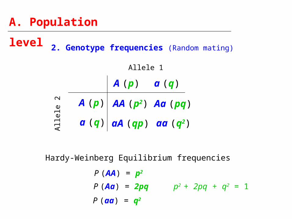
A. Population

level 2. Genotype frequencies (Random mating)

A (p) a (q)

A (p)

a (q)

Allele 1A

llele

2 AA (p2)

aA (qp)

Aa (pq)

aa (q2)

Hardy-Weinberg Equilibrium frequencies

P (AA) = p2

P (Aa) = 2pq

P (aa) = q2

p2 + 2pq + q2 = 1

Segregation, Meiosis

Mendel’s law of segregation

A3 (½) A4 (½)

A1 (½)

A2 (½)

Mother (A3A4)

A1A3 (¼)

A2A3 (¼)

A1A4 (¼)

A2A4 (¼)

Gametes

Father (A1A2)

B. Transmission level

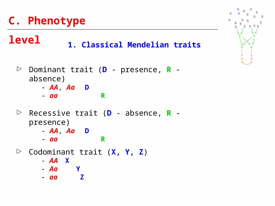
C. Phenotype

level 1. Classical Mendelian traits

Dominant trait (D - presence, R - absence) - AA, Aa D - aa R

Recessive trait (D - absence, R - presence) - AA, Aa D - aa R

Codominant trait (X, Y, Z) - AA X - Aa Y - aa Z

G

G

G

G

G

G

G

G

G

GG

G

G

G

G

G

GG

G

G

G

G

GG

PP

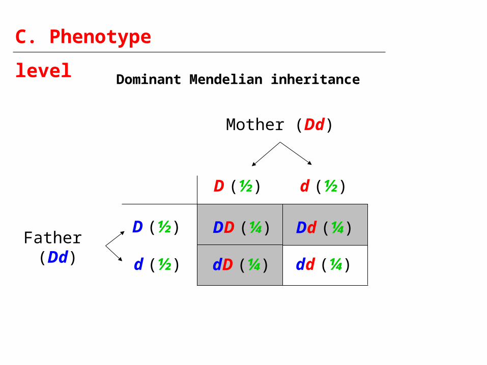
Dominant Mendelian inheritance

D (½) d (½)

D (½)

d (½)

Mother (Dd)

DD (¼)

dD (¼)

Dd (¼)

dd (¼)

Father (Dd)

C. Phenotype

level

D (½) d (½)

D (½)

d (½)

Mother (Dd)

DD (¼)

dD (¼)

Dd (¼)

dd (¼)Father (Dd)

Phenocopies

Incomplete penetrance

C. Phenotype

level Dominant Mendelian inheritance (with incomplete penetrance and phenocopies)

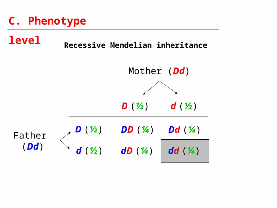
Recessive Mendelian inheritance

D (½) d (½)

D (½)

d (½)

Mother (Dd)

DD (¼)

dD (¼)

Dd (¼)

dd (¼)

Father (Dd)

C. Phenotype

level

2. Quantitative traits

Fra

ctio

n

Histograms by gqt

g==-1

0

.128205

g==0

-3.90647 2.7156g==1

-3.90647 2.7156

0

.128205

Fra

ctio

n

Histograms by gqt

g==-1

0

.128205

g==0

-3.90647 2.7156g==1

-3.90647 2.7156

0

.128205

Fra

ctio

n

Histograms by gqt

g==-1

0

.128205

g==0

-3.90647 2.7156g==1

-3.90647 2.7156

0

.128205

AA

Aa

aa

Fra

ctio

n

qt-3.90647 2.7156

0

.072

C. Phenotype

level

m

d +a

P(X)

X

AA

Aa

aa

m + a m + dm – a

– a

AAAaaa

Genotypic means

Biometric Model

Genotypic effect

C. Phenotype

level

3. Very basic statistical

concepts

Mean, variance,

covariance

i

iii

i

xfxn

xXE )(

1. Mean (X)

Mean, variance,

covariance

2. Variance (X)

iii

ii

xfxn

xXEXVar 2

2

2

1)()(

Mean, variance,

covariance

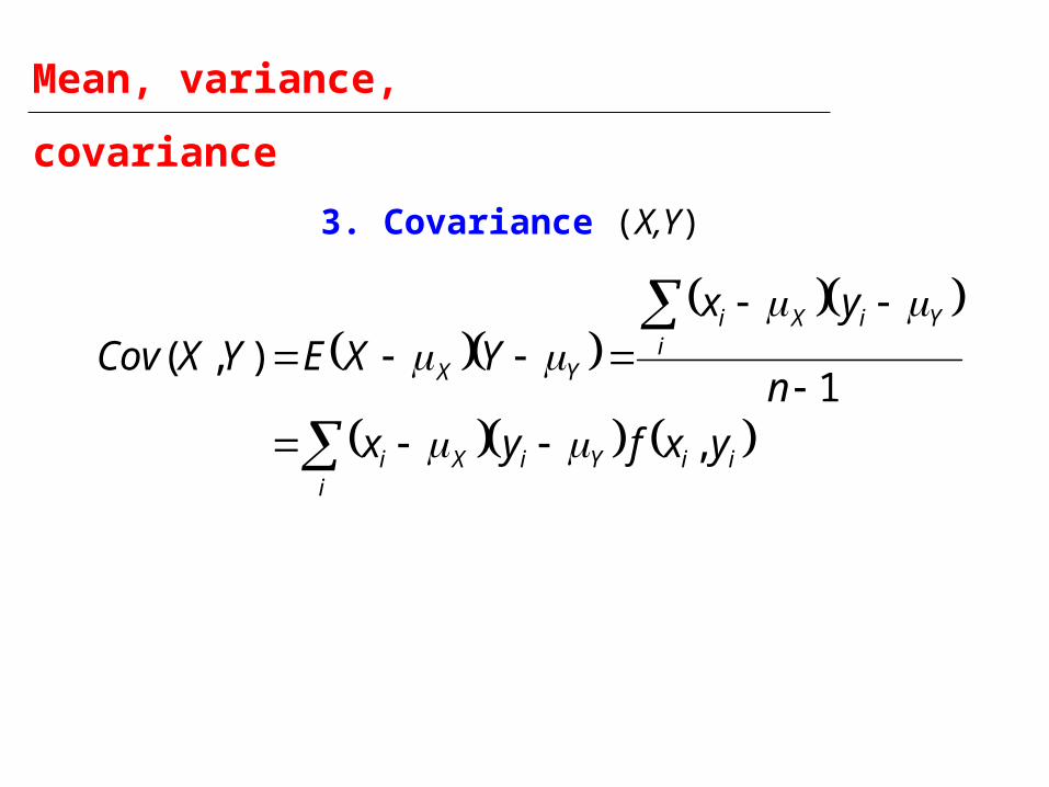
3. Covariance (X,Y)

iiiYiXi

iYiXi

YX

yxfyxn

yxYXEYXCov

,1

),(

4. Biometrical model

Biometrical model for single biallelic

QTLBiallelic locus - Genotypes: AA, Aa, aa - Genotype frequencies: p2, 2pq, q2

Alleles at this locus are transmitted from P-O according to Mendel’s law of segregation

Genotypes for this locus influence the expression of a quantitative trait X (i.e. locus is a QTL)

Biometrical genetic model that estimates the contribution of this QTL towards the (1) Mean, (2) Variance and (3) Covariance between individuals for this quantitative trait X

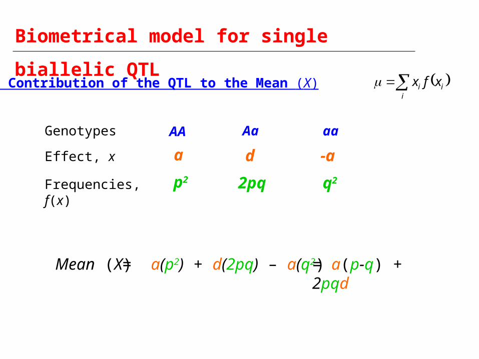
Biometrical model for single biallelic

QTL1. Contribution of the QTL to the Mean (X)

aaAaAAGenotypes

Frequencies, f(x)

Effect, x

p2 2pq q2

a d -a

i

ii xfx

= a(p2) + d(2pq) – a(q2)Mean (X) = a(p-q) + 2pqd

Biometrical model for single biallelic

QTL2. Contribution of the QTL to the Variance (X)

aaAaAAGenotypes

Frequencies, f(x)

Effect, x

p2 2pq q2

a d -a

= (a-m)2p2 + (d-m)22pq + (-a-m)2q2 Var (X)

i

ii xfxVar 2

= VQTL

Broad-sense heritability of X at this locus = VQTL / V Total

Broad-sense total heritability of X = ΣVQTL / V Total

Biometrical model for single biallelic

QTL = (a-m)2p2 + (d-m)22pq + (-a-m)2q2 Var (X)

= 2pq[a+(q-p)d]2 + (2pqd)2

= VAQTL + VDQTL

m

d +a– a

AAaa

Aa

Additive effects: the main effects of individual alleles

Dominance effects: represent the interaction between alleles

d = 0

Biometrical model for single biallelic

QTL = (a-m)2p2 + (d-m)22pq + (-a-m)2q2 Var (X)

= 2pq[a+(q-p)d]2 + (2pqd)2

= VAQTL + VDQTL

m

d +a– a

AAaa

Aa

Additive effects: the main effects of individual alleles

Dominance effects: represent the interaction between alleles

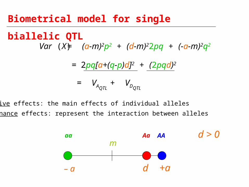
d > 0

Biometrical model for single biallelic

QTL = (a-m)2p2 + (d-m)22pq + (-a-m)2q2 Var (X)

= 2pq[a+(q-p)d]2 + (2pqd)2

= VAQTL + VDQTL

m

d +a– a

AAaa

Aa

Additive effects: the main effects of individual alleles

Dominance effects: represent the interaction between alleles

d < 0

Biometrical model for single biallelic

QTL

aa Aa AA

m

-a

ad

Var (X) = Regression Variance + Residual Variance= Additive Variance + Dominance Variance

PracticalH:\ferreira\biometric\sgene.exe

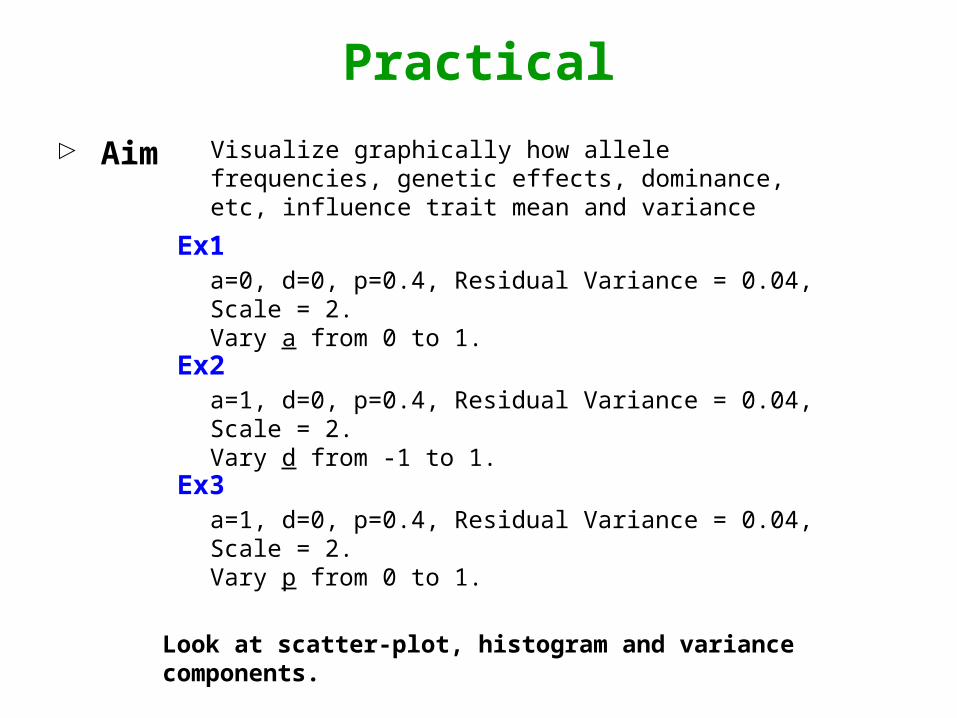
Practical

Aim Visualize graphically how allele frequencies, genetic effects, dominance, etc, influence trait mean and variance

Ex1a=0, d=0, p=0.4, Residual Variance = 0.04, Scale = 2.Vary a from 0 to 1.

Ex2a=1, d=0, p=0.4, Residual Variance = 0.04, Scale = 2.Vary d from -1 to 1.

Ex3a=1, d=0, p=0.4, Residual Variance = 0.04, Scale = 2.Vary p from 0 to 1.

Look at scatter-plot, histogram and variance components.

Some conclusions

1. Additive genetic variance depends on

allele frequency p

& additive genetic value a

as well as

dominance deviation d

2. Additive genetic variance typically greater than dominance variance

Biometrical model for single biallelic

QTLVar (X)= 2pq[a+(q-p)d]2 + (2pqd)2

VAQTL + VDQTL

Demonstrate

2A. Average allelic effect

2B. Additive genetic variance

Biometrical model for single biallelic

QTL2A. Average allelic effect (α)

The deviation of the allelic mean from the population mean

a(p-q) + 2pqd

Aaαa αA

? ?Mean (X)

Allele a Allele APopulation

AA Aa aaa d -a

A p q ap+dq q(a+d(q-p))

a p q dp-aq -p(a+d(q-p))

Allelic mean Average allelic effect (α)

1/3

Biometrical model for single biallelic

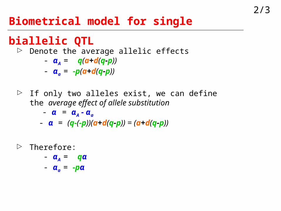
QTLDenote the average allelic effects - αA

= q(a+d(q-p)) - αa

= -p(a+d(q-p))

If only two alleles exist, we can define the average effect of allele substitution - α = αA - αa - α = (q-(-p))(a+d(q-p)) = (a+d(q-p))

Therefore: - αA

= qα - αa

= -pα

2/3

Biometrical model for single biallelic

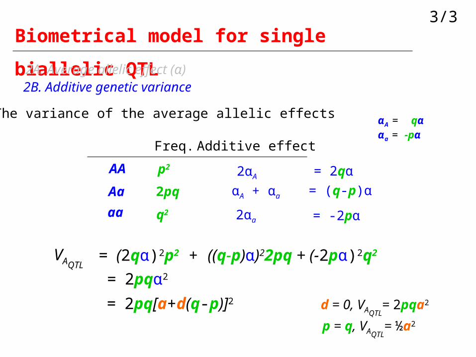
QTL2B. Additive genetic variance

The variance of the average allelic effects

2αA

Additive effect

2A. Average allelic effect (α)

Freq.

AA

Aa

aa

p2

2pq

q2

αA + αa

2αa

= 2qα

= (q-p)α

= -2pα

VAQTL= (2qα)2p2 + ((q-p)α)22pq + (-2pα)2q2

= 2pqα2

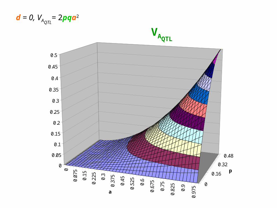
= 2pq[a+d(q-p)]2 d = 0, VAQTL= 2pqa2

p = q, VAQTL= ½a2

3/3

αA = qα

αa = -pα

0

0.07

5

0.15

0.22

5

0.3

0.37

5

0.45

0.52

5

0.6

0.67

5

0.75

0.82

5

0.9

0.97

5

0

0.16

0.32

0.48

0

0.05

0.1

0.15

0.2

0.25

0.3

0.35

0.4

0.45

0.5

a

p

d = 0, VAQTL= 2pqa2

VAQTL

-1

-0.8

-0.6

-0.4

-0.2 0

0.2

0.4

0.6

0.8 1

-1

-0.5

0

0.5

1

0

0.1

0.2

0.3

0.4

0.5

0.6

0.7

0.8

0.9

1

-1

-0.8

-0.6

-0.4

-0.2 0

0.2

0.4

0.6

0.8 1

-1

-0.4

0.2

0.8

0

0.1

0.2

0.3

0.4

0.5

0.6

0.7

0.8

0.9

1

-1

-0.8

-0.6

-0.4

-0.2 0

0.2

0.4

0.6

0.8 1

-1

-0.5

0

0.5

1

0

0.1

0.2

0.3

0.4

0.5

0.6

0.7

0.8

0.9

1

-1

-0.8

-0.6

-0.4

-0.2 0

0.2

0.4

0.6

0.8 1

-1

-0.4

0.2

0.8

0

0.1

0.2

0.3

0.4

0.5

0.6

0.7

0.8

0.9

1-1

-0.8

-0.6

-0.4

-0.2 0

0.2

0.4

0.6

0.8 1

-1

-0.5

0

0.5

1

0

0.1

0.2

0.3

0.4

0.5

0.6

0.7

0.8

0.9

1

-1

-0.8

-0.6

-0.4

-0.2 0

0.2

0.4

0.6

0.8 1

-1

-0.4

0.2

0.8

0

0.1

0.2

0.3

0.4

0.5

0.6

0.7

0.8

0.9

1

0.01 0.05 0.1 0.2 0.3 0.5

-1

-0.8

-0.6

-0.4

-0.2 0

0.2

0.4

0.6

0.8 1

-1

-0.5

0

0.5

1

0

0.1

0.2

0.3

0.4

0.5

0.6

0.7

0.8

0.9

1

-1

-0.8

-0.6

-0.4

-0.2 0

0.2

0.4

0.6

0.8 1

-1

-0.4

0.2

0.8

0

0.1

0.2

0.3

0.4

0.5

0.6

0.7

0.8

0.9

1

-1

-0.8

-0.6

-0.4

-0.2 0

0.2

0.4

0.6

0.8 1

-1

-0.4

0.2

0.8

0

0.1

0.2

0.3

0.4

0.5

0.6

0.7

0.8

0.9

1

-1

-0.8

-0.6

-0.4

-0.2 0

0.2

0.4

0.6

0.8 1

-1

-0.5

0

0.5

1

0

0.1

0.2

0.3

0.4

0.5

0.6

0.7

0.8

0.9

1

-1

-0.8

-0.6

-0.4

-0.2 0

0.2

0.4

0.6

0.8 1

-1

-0.4

0.2

0.8

0

0.1

0.2

0.3

0.4

0.5

0.6

0.7

0.8

0.9

1

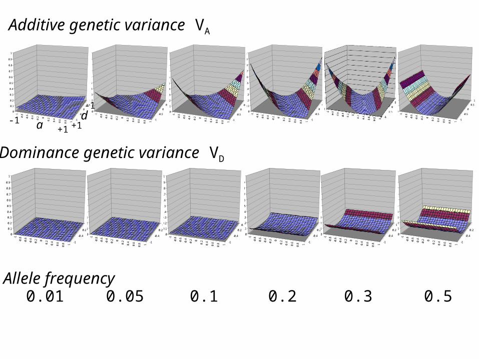
Allele frequency

Additive genetic variance VA

Dominance genetic variance VD

ad

+1-1

+1

-1

a

d

-1 0 +1

-1

0

+1

AA Aa aa

-1

-0.8

-0.6

-0.4

-0.2 0

0.2

0.4

0.6

0.8 1

-1

-0.9-0.8

-0.7-0.6

-0.5

-0.4-0.3

-0.2-0.1

0

0.10.2

0.30.4

0.5

0.60.7

0.80.9

1

-1

-0.8

-0.6

-0.4

-0.2 0

0.2

0.4

0.6

0.8 1

-1

-0.9-0.8

-0.7-0.6

-0.5

-0.4-0.3

-0.2-0.1

0

0.10.2

0.30.4

0.5

0.60.7

0.80.9

1

-1

-0.8

-0.6

-0.4

-0.2 0

0.2

0.4

0.6

0.8 1

-1

-0.9-0.8

-0.7-0.6

-0.5

-0.4-0.3

-0.2-0.1

0

0.10.2

0.30.4

0.5

0.60.7

0.80.9

1

-1

-0.8

-0.6

-0.4

-0.2 0

0.2

0.4

0.6

0.8 1

-1

-0.9-0.8

-0.7-0.6

-0.5

-0.4-0.3

-0.2-0.1

0

0.10.2

0.30.4

0.5

0.60.7

0.80.9

1

-1

-0.8

-0.6

-0.4

-0.2 0

0.2

0.4

0.6

0.8 1

-1

-0.9-0.8

-0.7-0.6

-0.5

-0.4-0.3

-0.2-0.1

0

0.10.2

0.30.4

0.5

0.60.7

0.80.9

1

-1

-0.8

-0.6

-0.4

-0.2 0

0.2

0.4

0.6

0.8 1

-1

-0.9-0.8

-0.7-0.6

-0.5

-0.4-0.3

-0.2-0.1

0

0.10.2

0.30.4

0.5

0.60.7

0.80.9

1

0.01 0.05 0.1 0.2 0.3 0.5Allele frequency

VA > VD

VA < VD

Biometrical model for single biallelic

QTL

2B. Additive genetic variance 2A. Average allelic effect (α)

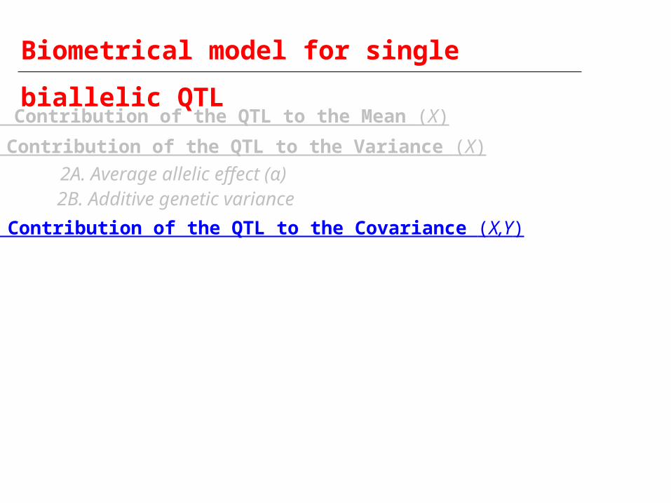
3. Contribution of the QTL to the Covariance (X,Y)

2. Contribution of the QTL to the Variance (X)

1. Contribution of the QTL to the Mean (X)

Biometrical model for single biallelic

QTL

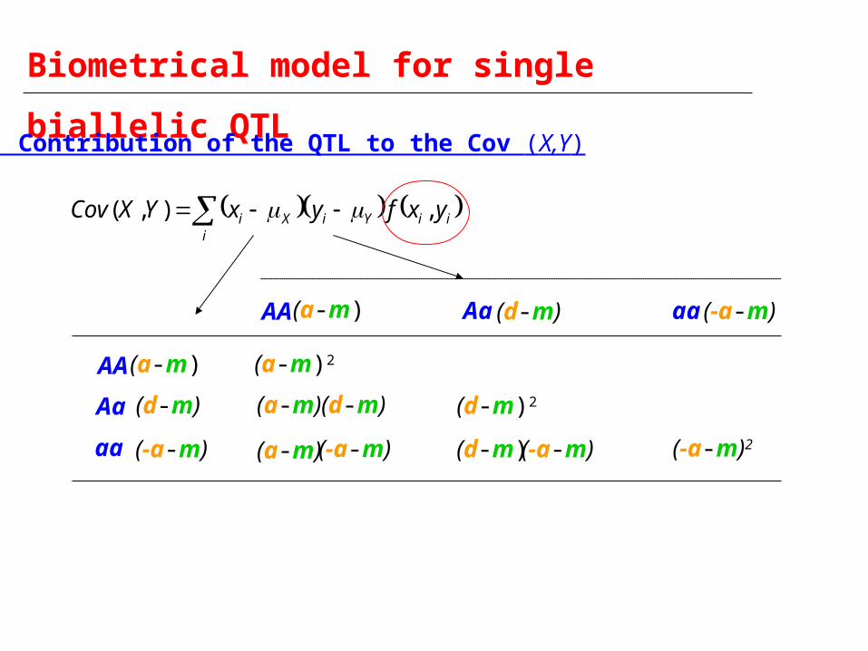
i

iiYiXi yxfyxYXCov ,),(

AA

Aa

aa

AA Aa aa(a-m) (d-m) (-a-m)

(a-m)

(d-m)

(-a-m)

(a-m)2

(a-m)

(-a-m)

(d-m)

(a-m)

(d-m)2

(d-m)(-a-m) (-a-m)2

3. Contribution of the QTL to the Cov (X,Y)

Biometrical model for single biallelic

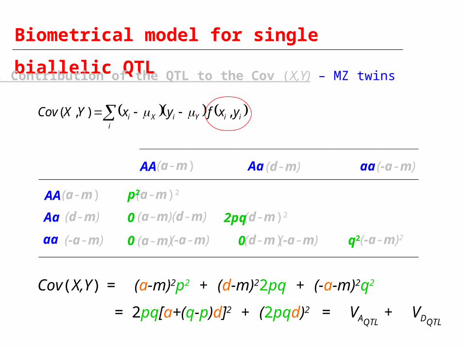
QTL

i

iiYiXi yxfyxYXCov ,),(

AA

Aa

aa

AA Aa aa(a-m) (d-m) (-a-m)

(a-m)

(d-m)

(-a-m)

(a-m)2

(a-m)

(-a-m)

(d-m)

(a-m)

(d-m)2

(d-m)(-a-m) (-a-m)2

p2

0

0

2pq

0 q2

3A. Contribution of the QTL to the Cov (X,Y) – MZ twins

= (a-m)2p2 + (d-m)22pq + (-a-m)2q2 Cov(X,Y)

= VAQTL + VDQTL

= 2pq[a+(q-p)d]2 + (2pqd)2

Biometrical model for single biallelic

QTL

AA

Aa

aa

AA Aa aa(a-m) (d-m) (-a-m)

(a-m)

(d-m)

(-a-m)

(a-m)2

(a-m)

(-a-m)

(d-m)

(a-m)

(d-m)2

(d-m)(-a-m) (-a-m)2

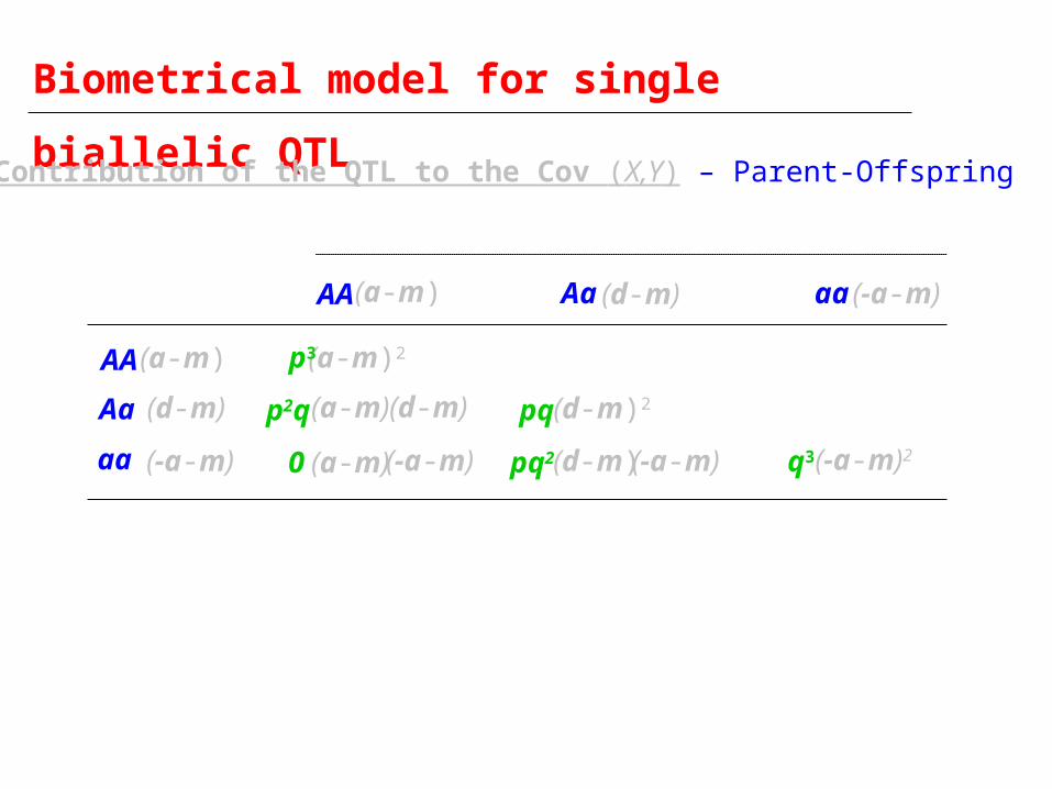
p3

p2q

0

pq

pq2 q3

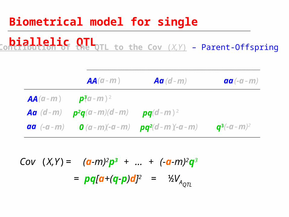
3B. Contribution of the QTL to the Cov (X,Y) – Parent-Offspring

• e.g. given an AA father, an AA offspring can come from either AA x AA or AA x Aa parental mating types

AA x AA will occur p2 × p2 = p4

and have AA offspring Prob()=1

AA x Aa will occur p2 × 2pq = 2p3q

and have AA offspring Prob()=0.5

and have Aa offspring Prob()=0.5

Therefore, P(AA father & AA offspring) = p4 + p3q

= p3(p+q)

= p3

Biometrical model for single biallelic

QTL

AA

Aa

aa

AA Aa aa(a-m) (d-m) (-a-m)

(a-m)

(d-m)

(-a-m)

(a-m)2

(a-m)

(-a-m)

(d-m)

(a-m)

(d-m)2

(d-m)(-a-m) (-a-m)2

p3

p2q

0

pq

pq2 q3

= (a-m)2p3 + … + (-a-m)2q3 Cov (X,Y)

= ½VAQTL= pq[a+(q-p)d]2

3B. Contribution of the QTL to the Cov (X,Y) – Parent-Offspring

Biometrical model for single biallelic

QTL

AA

Aa

aa

AA Aa aa(a-m) (d-m) (-a-m)

(a-m)

(d-m)

(-a-m)

(a-m)2

(a-m)

(-a-m)

(d-m)

(a-m)

(d-m)2

(d-m)(-a-m) (-a-m)2

p4

2p3q

p2q2

4p2q2

2pq3 q4

= (a-m)2p4 + … + (-a-m)2q4 Cov (X,Y)

= 0

3C. Contribution of the QTL to the Cov (X,Y) – Unrelated individuals

Biometrical model for single biallelic

QTL

Cov (X,Y)

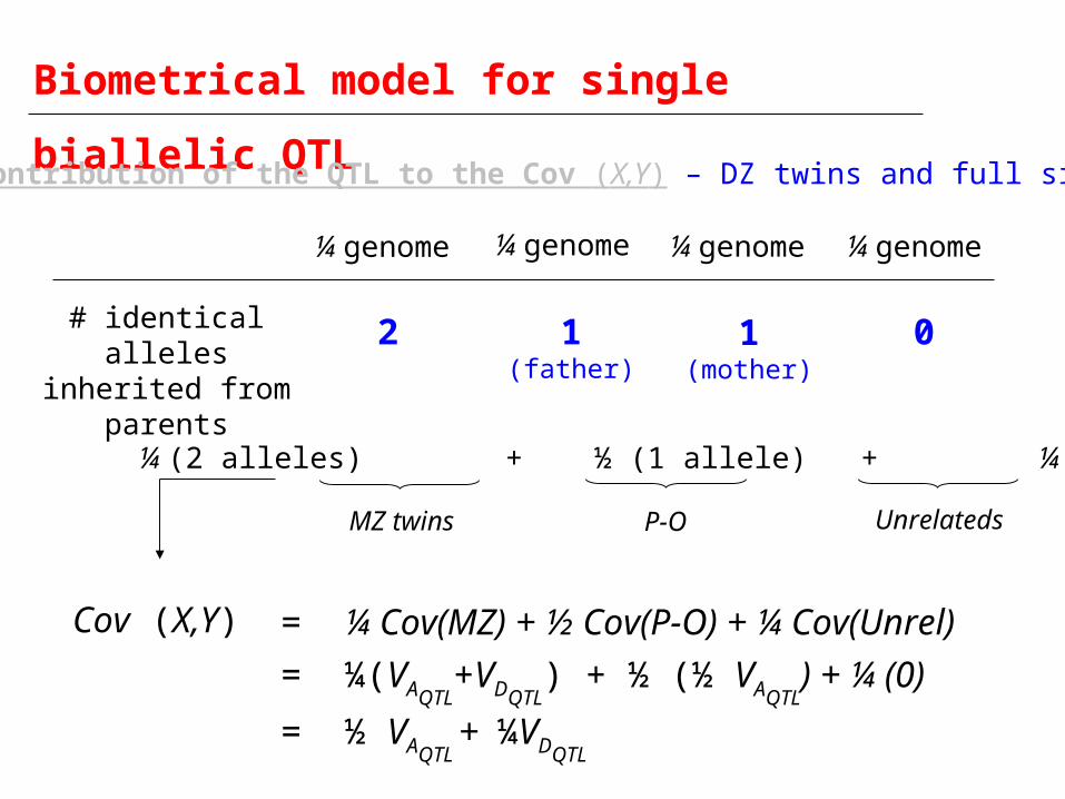
3D. Contribution of the QTL to the Cov (X,Y) – DZ twins and full sibs

¼ genome

¼ (2 alleles) + ½ (1 allele) + ¼ (0 alleles)

MZ twins P-O Unrelateds

¼ genome ¼ genome ¼ genome

# identical alleles inherited

from parents

01(mother)

1(father)

2

= ¼ Cov(MZ) + ½ Cov(P-O) + ¼ Cov(Unrel) = ¼(VAQTL

+VDQTL) + ½ (½ VAQTL

) + ¼

(0) = ½ VAQTL + ¼VDQTL

Summary

Biometrical model predicts contribution of a QTL to the mean, variance and covariances of a trait

Var (X) = VAQTL + VDQTL

1 QTL

Cov (MZ) = VAQTL + VDQTL

Cov (DZ) = ½VAQTL + ¼VDQTL

On average!

0 or 10, 1/2 or 1 IBD estimation /

Linkage

…Biometrical model underlies the variance components estimation performed in Mx, MERLIN, SOLAR, etc..

Var (X) = Σ(VAQTL) + Σ(VDQTL

) = VA + VDMultiple QTL

Cov (MZ)

Cov (DZ)

= Σ(VAQTL) + Σ(VDQTL

) = VA + VD

= Σ(½VAQTL) + Σ(¼VDQTL

) = ½VA +

¼VD