generic structures: exponential material delays · exponential delays in system dynamics are...
TRANSCRIPT

1 D-4614-F
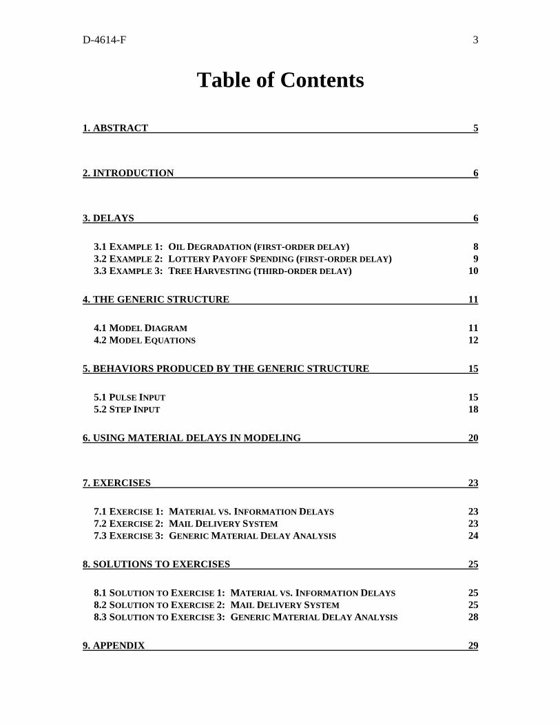
Generic Structures
Exponential Material Delays
Single Stock
outflow for single stockinflow for single stock
AVERAGE DELAY
INPUT
First-Order Material Delay
Prepared for theMIT System Dynamics in Education Project
Under the Supervision ofProf Jay W Forrester
byStephanie Albin
Copyright copy1998 by the Massachusetts Institute of TechnologyPermission granted to distribute for non-commercial educational purposes
6
D-4614-F 3
Table of Contents
1 ABSTRACT 5
2 INTRODUCTION
3 DELAYS
31 EXAMPLE 1 OIL DEGRADATION (FIRST-ORDER DELAY) 832 EXAMPLE 2 LOTTERY PAYOFF SPENDING (FIRST-ORDER DELAY) 933 EXAMPLE 3 TREE HARVESTING (THIRD-ORDER DELAY) 10
4 THE GENERIC STRUCTURE 11
41 MODEL DIAGRAM 1142 MODEL EQUATIONS 12
5 BEHAVIORS PRODUCED BY THE GENERIC STRUCTURE 15
51 PULSE INPUT 1552 STEP INPUT 18
6 USING MATERIAL DELAYS IN MODELING 20
7 EXERCISES
71 EXERCISE 1 MATERIAL VS INFORMATION DELAYS 2372 EXERCISE 2 MAIL DELIVERY SYSTEM 2373 EXERCISE 3 GENERIC MATERIAL DELAY ANALYSIS 24
8 SOLUTIONS TO EXERCISES 25
81 SOLUTION TO EXERCISE 1 MATERIAL VS INFORMATION DELAYS 2582 SOLUTION TO EXERCISE 2 MAIL DELIVERY SYSTEM 2583 SOLUTION TO EXERCISE 3 GENERIC MATERIAL DELAY ANALYSIS 28
9 APPENDIX 29
6
23
4 D-4614-F
91 EQUATIONS FOR EXAMPLE 1 OIL DEGRADATION MODEL 2992 EQUATIONS FOR EXAMPLE 2 LOTTERY PAYOFF SPENDING MODEL 3193 EQUATIONS FOR EXAMPLE 3 TREE HARVESTING MODEL 3194 EQUATIONS FOR SECTION 6 FACTORY-DISTRIBUTOR MODEL 33
5 D-4614-F
1 ABSTRACT
This paper introduces the generic structure of a material delay A material delay is
a delay in a physical flow In contrast an information delay is a delay in perception
All delays are characterized by two parameters the order of the delay and the
average length of the delay This paper uses Oil Degradation and Lottery Payoff Spending
models as examples of first-order delays A Tree Harvesting model is used as an example
of a third-order delay
After presenting the generic model diagram and equations this paper analyzes the
behaviors produced by the generic structure with various inputs The outflows to a first-
second- third- fourth- and infinite-order delay with pulse and step inputs are examined
After presenting a brief section containing hints to using material delays in
modeling this paper concludes with three exercises
6 D-4614-F
2 INTRODUCTION
Generic structures are relatively simple structures that recur in many diverse
situations In this paper for example spilled oil degradation inheritance spending and
tree harvesting systems are shown to share the same basic structure Transferability of
structure between systems makes the study of generic structures a fundamental part of
learning system dynamics
Road Maps contains a series of papers which use generic structures to develop an
understanding of the relationship between the structure and behavior of a system Such an
understanding should help one refine intuition about surrounding systems and improve
onersquos ability to model system behaviors
Knowledge about a generic structure in one system is transferable to understand
the behavior of other systems with the same structure Thus generic structures assist one
in understanding systems never studied before
This paper introduces the generic structure of material delays Many examples of
systems containing the material delay generic structure will be used to illustrate both the
transferability and functionality of the structure Soon the reader will be able to recognize
material delays in many new and different models
3 DELAYS
In real life the flow of non-physical information and physical material from one
place to another takes time Delivery of a package takes days and full comprehension of a
new idea can take years Delays are an inherent part of all flows Including a time delay in
every flow when building a system dynamics model however is impractical Often a
system delay is so short that its effect is negligible in comparison to longer or more
significantly located delays For example the delay in loading a delivery van is
insignificant to the delay in driving the van from its origin in New York to its destination
in California Through practice a modeler will learn to recognize which delays are
significant and which are not
7 D-4614-F
An delay is a stock-and-flow structure that accepts a given inflow and delivers a
resulting outflow A delay can be characterized as an exponential delay because in the
simplest form the outflow equals the stock divided by the average delay which
characteristically produces exponential decay1 Note that the outflow from the delay
structure is determined only by the stocks of the delay and by the average delay time The
inflow to the delay is independent of the delay structure Essentially a delay modifies the
time relationship between the inflow and outflow delay structure
Exponential delays in system dynamics are defined by two parameters the order
of the delay and the average length of the delay The order of the delay is the number of
stocks (or integrations) between the inflow and outflow of the delay structure The
average length of the delay is the average time between the initial input and the final
output The average length of the total delay is divided evenly among each stock in a
higher-order delay
Exponential delays can be divided into two categories material and information
A material delay modifies a physical flow while an information delay is a delay in
perception Under most conditions with identical inputs the output of a material delay is
identical to the output of an information delay The stock-and-flow structures are
however fundamentally different This paper will cover only material delays The reader
should keep in mind that a material delay does not lose or create any units of the flow
traveling through the delay structure Each unit that flows into the delay must either be
stored in a stock of the delay or flow out of the delay
Many software programs such as STELLA allow the modeler to define a
converter as a delay using special functions without explicitly modeling the stock-and-flow
structure While such short-cuts are useful the modeler must understand that all delays
contain stocks as part of the delay structure If the STELLA diagram contains a special
function converter defined as a delay then the diagram contains a stock within that
1 For more information see Stephanie Albin 1996 Generic Structures First order negative feedback loops (D-4475-1) System Dynamics Group Sloan School of Management Massachusetts Institute of Technology September 25 22 pp
8 D-4614-F
converter When simulating the model the software treats the delay converter as
containing a stock and carries out the appropriate integrations
9 D-4614-F
31 Example 1 Oil Degradation (first-order delay) 2
Figure 1 depicts a model of a simple pollution degradation system When oil is
spilled and contaminates a shoreline such as the Exxon Valdez spill that contaminated
Prince William Sound often the best course of action is to do nothing Adding additional
detergents or bacteria too speed up oil degradation may do more harm than good by
further damaging the natural habitat The oil will naturally disappear through a
combination of biodegradation evaporation and dissipation due to weather patterns The
stock ldquoOil Spilled on Shorerdquo represents the amount of oil spilled that reaches the shore
The oil accumulates at a rate equal to the ldquoOIL SPILLrdquo Through various factors
mentioned above the oil will degrade naturally at a rate equal to the ldquoOil Spilled on
Shorerdquo divided by the ldquoAVERAGE TIME TO DEGRADE OILrdquo After a certain length
of time (equal to the ldquoAVERAGE TIME TO DEGRADE OILrdquo) the oil levels on the
shore should be at minute non-toxic levels
Oil Spilled on Shore
natural degradation rateoil accumulation rate
OIL SPILL
AVERAGE TIME TO DEGRADE OIL
Figure 1 Oil Degradation Model
The degradation of oil a time-delayed process is the environmentrsquos response to an
oil spill The degradation of spilled oil is a material delay because it deals with the flow of
a material substance (the oil) into and out of a stock (the oil spilled on the shore) Figure
2 For equations of all example models please see appendix
10 D-4614-F
1 contains only one stock making the Oil Spill Degradation model a first-order material
delay
32 Example 2 Lottery Payoff Spending (first-order delay)
Figure 2 shows another example of a first-order material delay In the Lottery
Payoff Spending model a first-order material delay is used to represent the delay in
spending a large sum of money such as a lottery winning Often a person who has won a
large sum of money will spend large amounts of money the first few weeks and
substantially less as time goes on and the novelty of being a millionaire has worn off A
first-order delay is a good approximation of such behavior The stock ldquoMoney in Bank
Accountrdquo represents the delay between the time the money is won and the time the money
is spent The ldquomoney accumulation raterdquo equals the weekly ldquoLOTTERY WINNINGSrdquo
The winnings are spent each week at a ldquomoney spending raterdquo equal to the value of ldquoBank
Accountrdquo divided by the ldquoAVERAGE TIME TO SPEND WINNINGSrdquo
LOTTERY WINNINGS
Money in Bank Account
money accumulation rate money spending rate
AVERAGE TIME TO SPEND WINNINGS
Figure 2 Lottery Payoff Spending Model
Again the Lottery Payoff Spending model deals with the material flow of money
from being won to being spent The model is first-order because it only contains one
stock the inflow is only being delayed once by a single stock
D-4614-F 11
33 Example 3 Tree Harvesting (third-order delay)
The Tree Harvesting model in Figure 3 captures the dynamics of a tree farm where
a delay exists between the time a tree is planted and the time the tree is harvested The
length of the overall delay is the ldquoAVERAGE MATURATION TIMErdquo With three stocks
present in the delay the tree harvesting model contains a third-order delay In higher-
order delays (structures with two or more delay stocks) the convention is to spread the
delay evenly over each stock In the rate equations which flow out of a stock the
ldquoAVERAGE MATURATION TIMErdquo constant is divided by three The ldquosapling
maturation raterdquo equals ldquoSaplingsrdquo divided by one-third of the ldquoAVERAGE
MATURATION TIMErdquo The ldquomedium tree maturation raterdquo equals ldquoMedium Treesrdquo
divided by one-third of the ldquoAVERAGE MATURATION TIMErdquo The ldquoharvest raterdquo
equals ldquoHarvestable Treesrdquo divided by one-third of the ldquoAVERAGE MATURATION
TIMErdquo
AVERAGE MATURATION TIME
Saplings Medium Trees Harvestable Trees
planting rate sapling maturation rate
NUMBER PLANTED
medium tree maturation rate harvest rate
Figure 3 Tree Harvesting Model
ldquoNUMBER PLANTEDrdquo is simply the number of trees planted each year The
ldquoplanting raterdquo is equal to the ldquoNUMBER PLANTEDrdquo
Even though Figure 3 contains three stocks whereas Figures 1 and 2 contain only
one stock similarities in structure exist Each outflow equation is simply the stock divided
by the time constant scaled by the number of stocks in the delay The similarities exist
because all three example models contain the same material delay generic structure
12 D-4614-F
4 THE GENERIC STRUCTURE
This paper will now examine the generic structure of material delays used in all
three examples First two models of the generic structure first- and third-order will be
presented Then model equations for both cases will be examined
41 Model Diagram
Single Stock
inflow for single stock outflow for single stock
AVERAGE DELAY FOR FIRST ORDER DELAY
INPUT for first order delay
INPUT for third order delay
FIRST-ORDER DELAY
THIRD-ORDER DELAY
Stock 1 of 3 Stock 2 of 3 Stock 3 of 3
inflow for chain flow from stock 1 to 2 outflow for chainflow from stock 2 to 3
AVERAGE DELAY FOR THIRD ORDER DELAY
Figure 4 Generic Structures of a First- and Third-order Delay
Figure 4 contains the generic structures of first- and third-order delays Note that
to create a second- fourth- or higher-order delay one must either lengthen or shorten the
chain of stocks in the third-order delay model and put in the appropriate links from the
average delay converter to the flows Given any ldquoINPUTrdquo the models in Figure 4 will
create an appropriate delay of length equal to the ldquoAVERAGE DELAYrdquo between the
inflow and final outflow of the single stock or stock chain The behavior of the outflow
D-4614-F 13
will differ depending on the order of delay The different outflow curves will be examined
in a later section of this paper
42 Model Equations
FIRST-ORDER DELAY
INPUT_for_first_order_delay = a constant
DOCUMENT ldquoINPUT for first order delayrdquo is the input to the delay It can be a
constant a pulse a sine wave or any other function
UNIT Unittime
inflow_for_single_stock = INPUT_for_first_order_delay
DOCUMENT The inflow for a single stock is the input to the system It is the inflow
that undergoes the first-order time delay
UNIT Unittime
Single_Stock(t) = Single_Stock(t - dt) + (inflow_for_single_stock -
outflow_for_single_stock) dt
DOCUMENT This is the single stock in a first-order delay It corresponds to the stocks
of ldquoOil Spilled on Shorerdquo and ldquoMoney in Bank Accountrdquo in examples 1 and 2 This stock
holds the amount of material stored in the delay which is in transit between the inflow and
outflow for the stock
UNIT Unit
outflow_for_single_stock = Single_Stock
AVERAGE_DELAY_FOR_FIRST_ORDER_DELAY
DOCUMENT The outflow for a single stock is the delayed response of the input inflow
for a single stock
UNIT Unittime
14 D-4614-F
AVERAGE_DELAY_FOR_FIRST_ORDER_DELAY = a constant
DOCUMENT This is the average time it takes each unit to go from flowing into the
stock to flowing out of the stock
UNIT Time
THIRD-ORDER DELAY3
INPUT_for_third_order_delay = a constant
DOCUMENT ldquoINPUT for third order delayrdquo is the input to the delay It can be a
constant a pulse a sine wave or any other function
UNIT Unittime
inflow_for_chain = INPUT_for_third_order_delay
DOCUMENT The inflow for chain represents the inflow to the third-order delay
UNIT Unittime
Stock_1_of_3(t) = Stock_1_of_3(t - dt) + (inflow_for_chain - flow_from_stock_1_to_2)
dt
DOCUMENT This is the first stock in a chain of three stocks that constitute the third-
order delay This stock is delaying the ldquoinflow for chainrdquo and corresponds to ldquoSaplingsrdquo
in example 3
UNIT Unit
flow_from_stock_1_to_2 =
Stock_1_of_3(AVERAGE_DELAY_FOR_THIRD_ORDER_DELAY3)
DOCUMENT The ldquoflow from stock 1 to 2rdquo is the outflow of the first stock of the delay
chain and is the inflow for the remaining chain
UNIT Unittime
3 Mathematically any delay of order ldquonrdquo with an average delay equal to ldquoDrdquo is equivalent to ldquonrdquo cascaded first-order delays each having an average delay equal to ldquoDnrdquo
D-4614-F 15
Stock_2_of_3(t) = Stock_2_of_3(t - dt) + (flow_from_stock_1_to_2 -
flow_from_stock_2_to_3) dt
DOCUMENT ldquoStock 2 of 3rdquo stores part of the input material that is being delayed This
stock is further delaying the already-delayed material transferred by ldquoflow from stock 1 to
2rdquo ldquoStock 2 of 3rdquo corresponds to ldquoMedium Treesrdquo in example 3
UNIT Unit
flow_from_stock_2_to_3 =
Stock_2_of_3(AVERAGE_DELAY_FOR_THIRD_ORDER_DELAY3)
DOCUMENT The ldquoflow from stock 2 to 3rdquo is the outflow of the second stock of the
delay chain and is the inflow for the remaining chain
UNIT Unittime
Stock_3_of_3(t) = Stock_3_of_3(t - dt) + (flow_from_stock_2_to_3 shy
outflow_for_chain) dt
DOCUMENT ldquoStock 3 of 3rdquo accumulates the already-delayed outflow from stock 2 and
delays it again ldquoStock 3 of 3rdquo corresponds to the ldquoHarvestable Treesrdquo in example 3
UNIT Unit
outflow_for_chain =
Stock_3_of_3(AVERAGE_DELAY_FOR_THIRD_ORDER_DELAY3)
DOCUMENT The outflow for the entire chain is a delayed appearance of the ldquoINPUT
for third order delayrdquo material inflow for the chain
UNIT Unittime
AVERAGE_DELAY_FOR_THIRD_ORDER_DELAY = a constant
DOCUMENT This is the average time it takes for each unit from flowing into to flowing
out of the entire chain It is important to note that the total ldquoAVERAGE DELAY FOR
16 D-4614-F
THIRD ORDER DELAYrdquo is spread out over all three stocks of the delay Division by 3
in each of the outflow equations is necessary to accurately capture the average delay
UNIT time
5 BEHAVIORS PRODUCED BY THE GENERIC STRUCTURE
The transient response of a material delay changes as the number of stocks in the
delay is increased This section will examine the transient responses of first- second-
third- and fourth-order delays to various inputs
51 Pulse Input
The STELLA software has a built-in function called ldquoPULSErdquo This paper will
use the PULSE function as an input to material delays of various orders and will graph
and analyze the resulting outputs
The PULSE function generates an input of a specified size at a specified time for a
length of time equal to the simulation time step (DT) of the model The PULSE function
in STELLA takes the form
PULSE(ltvolumegt[ ltfirst pulsegt ltintervalgt])
The height of the pulse equals the volume divided by DT If for example a volume of 10
is pulsed with a simulation DT set to 025 time-units the actual number of units pulsed is
10025 which equals 40 units The pulse of 40 units lasts 025 time-units of the model If
the PULSE(10 0 9999) with a DT of 025 were the inflow to a stock (initial value equal
to zero) then the value of the stock after the first time step would be 10 units The rate of
inflow would equal 40 units but only for 025 time-units resulting in a stock value of only
40 025 or 10 units First pulse specifies the time at which the first pulse occurs
Interval is the period of time between subsequent pulses If only one initial pulse is
desired the interval value should be set to a number that is greater than the maximum
length of simulation 9999 years is greater than any of the simulation lengths that will be
used in this paper
D-4614-F 17
1 INPUT 2 1st order outflow 3 2nd order outflow 4 3rd order outflow 5 4th order outflow 1 2 3 4 5
1 2 3 4 5
1 2 3 4 5
100000 1000
50000
500
000
000
1
5 1 3 4
2 5
1 2 3
41
1 1
2 3 4
5 1
2 3 4 5
-500 500 1500 2500 3500
time-unit PULSE at time = 0
Figure 5 Outflows for First- Second- Third- and Fourth-Order Delays4
Figure 5 contains a graph of the outflows of first- second- third- and fourth-
order delays5 The initial inflow for each delay is a pulse of 1000 units of material over 01
time-units With a DT of 01 the volume of the pulse is thus 100 units The exact
equation of the ldquoINPUTrdquo for the STELLA models is INPUT = PULSE(100 0 9999)
which creates a pulse of 1000 units at time zero The initial level of each stock was set to
zero and the average delay for each material delay was set to 10 time-units Note that the
delay is divided evenly among each of the flows in a higher-order delay
The pulse input is simply depositing 100 units of material into the delay chain at
time zero Imagine the inflow of the delay as 100 items inserted into a transportation
system at one moment and the outflow of the delay as the rate of arrival of the items at
their destinations
4 The time scale of the graph in Figure 7 begins at -5 time-units so that the PULSE input at time 0 can be easily seen 5 The structures used for the first- and third-order delays are identical to those presented in Figure 4 The structures for the second- and fourth-order delays are similar varying only by the number of stocks present
18 D-4614-F
Curve 2 in Figure 5 shows the outflow of a first-order exponential delay From the
graph one can see that the maximum rate of output occurs immediately after the pulse
input and the outflow decreases exponentially thereafter
For the second-order delay outflow curve 3 the initial outflow is zero because the
entire input is momentarily stored in the first stock of the two-stock delay chain The level
of the second stock is thus zero immediately after the pulse so there can be no outflow
from it Note also that the output curve has its maximum slope at the origin The
maximum slope occurs at the origin because the second stock of the two-stock delay chain
is delaying the outflow from the first stock The outflow from the first stock is an
exponential decay similar in shape to curve 2 and has the maximum value immediately
after time zero
Curve 4 the outflow of a third-order material delay has an initial output of zero
and an initial slope also of zero The outflow curve begins to rise slowly reaches a
maximum slope and a peak value and then falls off The third-order delay outflow peaks
higher and later in time than the second-order delay outflow The third stock of the three-
stock delay chain acts like a first-order delay with an input similar in shape to curve 3
The initial slope equals zero because the initial input to the third-stock of the delay chain is
zero
The fourth-order delay curve is very much like the third-order delay curve The
fourth-order outflow curve also begins with a value of zero and a slope equal to zero
characteristics that are shared by all higher-order curves Again the fourth-order outflow
peaks higher in magnitude but later in time than the third-order outflow curve From
Figure 5 one can observe that as the order of the delay increases the outflow peaks at a
higher value and at a time that is closer to the average delay time Continuing along
similar lines of reasoning the ultimate end member of the delay family is the hypothetical
infinite-order delay6 An infinite-order delay also known as a discrete or pipeline delay is
shown in Figure 6
6 Jay W Forrester 1961 Industrial Dynamics (p 86-92) Portland OR Productivity Press 464 pp
D-4614-F 19
1 INPUT 2 infinite order outflow 100000
50000
1
2
1
1
2 1 2
2
AVERAGE DELAY
1 2 1 2 -500 500 1500 2500 3500
time-unit PULSE at time = 0
Figure 6 Outflow for Infinite-Order Delay
The outflow of the infinite-order delay is zero until at a time equal to the average
delay the entire pulse input flows out of the delay chain To model an infinite-order delay
in STELLA one can use the built-in DELAY function The DELAY function takes the
form
DELAY(ltinputgt ltdelay durationgt [ltinitialgt])
The delay outflow in Figure 6 was created with the identical pulse ldquoINPUTrdquo used in
Figure 5 a delay duration or average delay equal to 10 and an initial delay value of zero
for the stocks in the infinite-chain In STELLA the equation for the converter ldquoinfinite
order outflowrdquo equals DELAY(INPUT 10 0) As one can see the amount of material
pulsed into the delay is conserved as that same volume is pulsed out at a time equal to the
average delay
The model of an infinite-order delay is simply the ldquoINPUTrdquo converter connected
by an information link to a converter whose equation is the DELAY function as described
above Even though the model diagram does not contain any stocks the stocks of the
delay are internal to the second converter STELLA simulates the two-converter model as
if it were a model containing an infinitely long chain of stocks
000
20 D-4614-F
52 Step Input
The STELLA software also has a built-in function called ldquoSTEPrdquo This section
will use the STEP function as an input to material delays of various orders and the output
will be graphed and analyzed
The STEP function generates a step input of a specified size or height at a
specified time The input to the STEP function is in the form
STEP(ltheightgt lttimegt)
For the graphs in Figures 7 and 8 a STEP of 100 units of material flows into the delay at
time 0 The INPUT equals STEP(100 0) and each delay-chain has an average delay of
10 time-units and the stocks had an initial value of zero Figure 7 graphs the outflows
resulting from the STEP input to a first- second- third- and fourth-order delay
1 INPUT 2 1st order outflow 3 2nd order outflow 4 3rd order outflow 5 4th order outflow 1 1 1 510000
5000
000 1 2
2
2
2
3
3
3
3
4
4
4 4
5
5
5
AVERAGE DELAY
-500 500 1000 1500 2500 3500
time-unit STEP at time = 0
Figure 7 Outflows for First- Second- Third- and Fourth-Order Delays
Curve 2 represents the output of a first-order material exponential delay in
response to a STEP input at time zero equal to 100 units The first-order outflow is an
exponential rise in outflow of the units of material The area between the ldquoINPUTrdquo curve
1 and the first-order output curve 2 is a measure of the number of units that accumulate in
D-4614-F 21
the delay stock For the first-order delay graphed in Figure 7 the ldquoINPUTrdquo is constant
and equal to 100 units resulting in a total output (the outflow summed over time) which is
less than the total input (the ldquoINPUTrdquo summed over time) by the number of units stored in
the delay stock It is also important to note that the first-order outflow curve has its
maximum slope at the time of the STEP
Curve 3 the outflow of a second-order delay in response to a STEP input curve
4 the outflow of a third-order delay and curve 5 the outflow of a fourth-order delay all
have the same basic S-shape The outflow curves 3 4 and 5 initially have a slope of zero
because the outflow from the first stock in the chain equals zero The slope then increases
at first and then decreases as the outflow asymptotically approaches the level of input
Mathematically the outflow of an exponential material delay of any order (with the
exception of an infinite-order delay) will never ldquoreachrdquo the value of the inflow but the
difference is so small in magnitude that the effect is usually insignificant Also as the
order of the delay (greater than second-order) increases the point of time at which the
slope changes from increasing to decreasing approaches the average delay time
The outflow of an infinite-order delay in response to the identical STEP input is
shown in Figure 8 The input step rises suddenly from zero to its final value and the
infinite-order delay steps from zero to final value at 10 time-units later The outflow
mirrors the step input after a time shift equal to the average delay time
22 D-4614-F
1 INPUT 2 infinite order outflow 10000
5000
000 -500 500 1500 2500 3500
time-unit
1
1 1 1
2 2
2 2
AVERAGE DELAY
STEP at time = 0
Figure 8 Outflow for Infinite-Order Delay
6 USING MATERIAL DELAYS IN MODELING
Material delays exist in many diverse systems such as a mail delivery system
breakdown of a radioactive isotope or construction of buildings In order to best
approximate the order of a delay in a system dynamics model a modeler must consider the
systemrsquos real-life behavior The shape of the systemrsquos real-life delayed outflow should be
approximated by the material delayrsquos outflow Consider the delay in shipping goods from
a factory to distributors7 Think of a large shipment of simultaneous orders (a ldquopulserdquo)
that is being transported from a factory to its distributors and try to characterize the delay
in the rate of arrival to the distributor
Figures 5 and 6 show the outflows of a pulse input to first- second- third- fourthshy
and infinite-order delays A modeler can consider the curves in Figures 5 and 6 to be
possible rates of arrival of a good with the ldquoINPUTrdquo equaling the large shipment of
simultaneous orders The outflow curve of a first-order material delay in response to a
pulse input is an exponentially decreasing curve with the maximum rate of arrival of the
7 Jay W Forrester 1961 Industrial Dynamics (p 89-92) Portland OR Productivity Press 464 pp
D-4614-F 23
good at the instant the shipments are made Because the maximum rate of arrival of a
good does not occur at the moment the goods have been shipped the first-order delay
should be eliminated as a possible structure in the factory-distributor model
The second-order delay outflow curve in Figure 5 has a zero rate of outflow at
time zero Similarly our example system has a zero rate of arrival at the time the
shipments are made The second-order delay outflow curve however has its maximum
slope at the origin which is unrealistic in the factory-distributor system One does not
expect the rate of arrivals to rise rapidly at the moment the shipments leave the factory
Now consider the infinite-order delay outflow curve in Figure 6 Because the
goods being shipped do not all arrive at the distributors at the same instant the infinite-
order delay possibility can be eliminated
The delay outflow curves in Figure 5 for the third- and fourth-order delay both
contain the necessary requirements of an arrival rate of zero at the time the shipments are
made and a slowly increasing arrival rate of goods Choosing between third- and higher-
order delays means studying the actual rate of arrival carefully and picking the order of
delay that most closely matches the behavior of the system In most cases however the
extra precision gained from an intensive study of the real system will not have an
appreciable effect on model behavior and the cost of such a study will not be worthwhile
Goods in Factory Goods at DistributorGoods in Transit 1
arrival rate of goodsshipment rate of goods flow 1 to 2
Goods in Transit 2 Goods in Transit 3
flow 2 to 3
AVERAGE DELAY FROM FACTORY TO DISTRIBUTOR
Figure 9 Factory - Distributor Model8
Figure 9 contains a model of a factory-distributor system The three stocks of the
third-order delay are ldquoGoods in Transit 1rdquo ldquoGoods in Transit 2rdquo and ldquoGoods in Transit
8 Equations for the Factory-Distributor Model are located in Section 94 of the Appendix
24 D-4614-F
3rdquo The actual names of the three delay stocks are unimportant because the modeler is
only interested in the ldquoarrival rate of goodsrdquo If the goods were being shipped from a
factory in Mexico to a distributor in Canada through the United States for example the
names of the delay stocks could be ldquoGoods in Californiardquo ldquoGoods in Oregonrdquo and
ldquoGoods in Washingtonrdquo The ldquoarrival rate of goodsrdquo will be the outflow of a third-order
delay with an input of the ldquoshipment rate of goodsrdquo regardless of the names of the internal
delay stocks and flows
Some system dynamics modeling software programs have built-in functions for
material delays where the modeler can specify the average delay and the order of the delay
without needing to explicitly model the stock-and-flow delay structure Consult the
technical manual of the particular modeling software used for more information
D-4614-F 25
7 EXERCISES
The following exercises provide the reader with a chance to apply and practice using the
generic structure of a material delay Solutions are located in section 8 of this paper
71 Exercise 1 Material vs Information Delays
Section 31 of this paper briefly explained the difference between material and
information delays Remember a material delay modifies a physical flow Information
delays are delays in perception Below is a list of systems in which some flow is being
delayed Which are material delays Which are information delays
1 Delay in production of applesauce from harvested apples
2 Delay in firing team manager when sports team loses games
3 Delay in arrival of mail
4 Delay in the increased number of carpools due to an increase in price of gas
5 Delay in growth of ripe tomatoes from a tomato plant seed
6 Delay in making a decision after collecting necessary data
72 Exercise 2 Mail Delivery System
Rachel and Ross are getting married They want to get married as soon as
possible but they are afraid that if they pick a day too soon their invitations will not be
delivered on time To help them pick a date they have asked you to build a system
dynamics model of the mail system
Assume it takes an average of 3 days for any invitation to get sorted at the post-
office of origin transported and sorted again at the destination post-office Rachel and
Ross are sending out 200 invitations and would be satisfied if 175 of them were delivered
the day before the wedding Try carrying out the same type of analysis done in section 6
of this paper to help build the delay structure of the mail delivery model Use a PULSE
function input on day zero as the depositing of 200 invitations into the mail system What
is the earliest day when Rachel and Ross can get married if the invitations are sent out on
February 8th
D-4614-F 27
73 Exercise 3 Generic Material Delay Analysis
Consider the following two generic delay structures
Delay Structure 1 A third-order delay with an average delay length of 20 time-units
Delay Structure 2 Three cascaded first-order delays forming a chain The first delay has
an average delay of 1 time-unit the second delay has an average delay of 1 time-unit and
the third-delay has an average delay of 18 time-units Note these three average delays add
up to 20 time-units the average delay length of Delay Structure 1
Figure 10 contains a picture of the two structures but the model diagram is not
necessary to solve this exercise
AVERAGE DELAY FOR THIRD ORDER DELAY
Delay Stock 1 of 3
flow of stock 1 to 2
Delay Stock 1
Delay Stock 2 of 3
flow of stock 2 to 3
Delay Stock 2
Delay Stock 3 of 3
outflow of third order delay
Delay Stock 3
flow of 1 to 2 flow of 2 to 3 outflow of 3 first order delays
INPUT
inflow to third order delay
inflow to 3 first order delays
AVERAGE DELAY 1 AVERAGE DELAY 2 AVERAGE DELAY 3
Figure 10 Stock-and-flow Diagram of Delay Structures 1 and 2
Answer the following questions assuming an initial INPUT pulse of 100 units of material
1 Will the outflow curves for the third-order delay structure be identical to the outflow
of the chain of three first-order delays
2 Which outflow curve will have a higher peak Which outflow curve will peak at a
time closer to 20 time-units Why
28 D-4614-F
8 SOLUTIONS TO EXERCISES
81 Solution to Exercise 1 Material vs Information Delays
1 Material (delay in the physical flow of apples from tree to factory through mashing
machines)
2 Information (delay in the realization that the team is on a losing streak due to bad
management)
3 Material (delay in the physical flow of letters due to sorting and transportation)
4 Information (delay in realization that the increase in gas prices is permanent and to join
a carpool is more economical)
5 Material (delay in maturation of a seed to a fruit-bearing plant)
6 Information (delay in analyzing data to making the final decision based on the data)
82 Solution to Exercise 2 Mail Delivery System
Following the same reasoning presented in Section 6 as to why the ldquoarrival rate of goodsrdquo
is the outflow to a third-order delay the ldquomail delivery raterdquo is also a third-order material
delay outflow The model diagram in Figure 11 contains a third-order delay with stocks
of ldquoMail Sorted at Post Office 1rdquo ldquoMail in Transitrdquo and ldquoMail Sorted at Post Office 2rdquo
Note that the names of the three delay stocks are unimportant and the exercise focuses on
the number of delivered invitations as the important variable of the system The equations
at the end of this subsection in particular the equation of ldquomail deposit raterdquo were
selected with a DT of 025 For the Mail Delivery System the ldquomail deposit raterdquo equals
800 invitationsday at day zero but only lasts one-quarter day The ldquomail deposit raterdquo
then dumps in exactly 200 invitations into the ldquoMail Sorted at Post Office 1rdquo stock
D-4614-F 29
Mail Sorted at Post Office 1 Mail in Transit Mail Sorted at Post Office 2 Delivered Mail
mail delivery ratemail deposit rate rate of mail flow 1 rate of mail flow 2
AVERAGE DELAY FOR MAIL DELIVERY
Figure 11 Mail Deliver System
1 Mail Sorted at Post Office 1 2 Delivered Mail
000 200 400 600 800 000
10000
20000
1
1
1 12
2
2
2
500
175
Days
Figure 12
From the graph in Figure 12 a simulation run of the model in Figure 11 it is obvious that
175 invitations will be delivered by the fifth day after mailing the invitations Rachel and
Ross should have their wedding one day latermdash on February 14th Valentinersquos Day
Equations
mail_deposit_rate = PULSE(20009999)
DOCUMENT The pulse function is used to represent the deposit of 200 wedding
invitations into the mailbox DT is set to 025 so the number of invitations pulsed into the
first stock of the delay equals 200
30 D-4614-F
UNIT Invitation
Mail_Sorted_at_Post_Office_1(t) = Mail_Sorted_at_Post_Office_1(t - dt) +
(mail_deposit_rate - rate_of_mail_flow_1) dt
INIT Mail_Sorted_at_Post_Office_1 = 0
DOCUMENT The first stock of the delay
UNIT Invitation
rate_of_mail_flow_1 =
Mail_Sorted_at_Post_Office_1(AVERAGE_DELAY_FOR_MAIL_DELIVERY3)
DOCUMENT The flow of invitations from the post office of origin to a mail truck en
route
UNIT Invitationday
Mail_in_Transit(t) = Mail_in_Transit(t - dt) + (rate_of_mail_flow_1 -
rate_of_mail_flow_2) dt
INIT Mail_in_Transit = 0
DOCUMENT The second stock of the delay
UNIT Invitation
rate_of_mail_flow_2 =
Mail_in_Transit(AVERAGE_DELAY_FOR_MAIL_DELIVERY3)
DOCUMENT The flow of invitations from the mail in trucks to being sorted mail at the
post-office
UNIT Invitationday
Mail_Sorted_at_Post_Office_2(t) = Mail_Sorted_at_Post_Office_2(t - dt) +
(rate_of_mail_flow_2 - mail_delivery_rate) dt
INIT Mail_Sorted_at_Post_Office_2 = 0
DOCUMENT The third stock of the delay
D-4614-F 31
UNIT Invitationday
mail_delivery_rate =
Mail_Sorted_at_Post_Office_2(AVERAGE_DELAY_FOR_MAIL_
DELIVERY3)
DOCUMENT The rate of arrival of invitations after a third-order delay
UNIT Invitationday
Delivered_Mail(t) = Delivered_Mail(t - dt) + (mail_delivery_rate) dt
INIT Delivered_Mail = 0
DOCUMENT The stock of delivered mail is not part of the third-order delay and
represents the mail that has been successfully delivered
UNIT Invitation
AVERAGE_DELAY_FOR_MAIL_DELIVERY = 3
DOCUMENT The average time it takes one invitation of Rachel and Ross to reach its
destination The average delay time is divided evenly over the three stocks of the delay
UNIT Day
83 Solution to Exercise 3 Generic Material Delay Analysis
1 The two outflows are not identical
2 The outflow of the three first-order delays will peak higher than the outflow of the
third-order delay The higher peak is also further away from 20 time-units An actual
simulation of the two structures shown in Figure 13 verifies that the outflow from the
three first order delays peaks higher and earlier than the outflow of the third-order delay
The behavior of the two outflow curves can be explained by considering the time
one is dividing by in each internal flow equation For the third-order delay each stock is
being divided by one-third the total average delay (20 time-units 3) Each third-order
delay stock is thus being divided by 667 time-units
32 D-4614-F
For the outflow of the third-order delay the material is being delayed the same
amount of time 667 time-units in each stock For the outflow of the three first-order
delays the material is only being delayed a short time one time-unit in each of the first
two stocks in the chain The outflow rate for the three first-order delays will thus peak
earlier because the material is being pumped through the first two stocks of the chain
rather quickly More material will reach the last stock of the three first-order delays chain
than the last stock of the third-order delay so the peak occurs earlier in time
The easiest way to think about exercise 3 is to realize that the chain of three first-
order delays is behaving almost like a single first-order delay of 20 time-units The
previous statement is verified by examining the graph in Figure 13 Notice that the
ldquooutflow of 3 first order delaysrdquo curve looks very much like the exponential decay outflow
curve of a single first-order delay examined in Figure 5
1 outflow of third order delay 2 outflow of 3 first order delays 1 2
1 2
1 2
500
250
000
2 1
2 1
2
1
1 2
000 1250 2500 3750 5000
Time
Figure 13 Outflow of the two structures in exercise 3
D-4614-F 33
9 APPENDIX
91 Equations for Example 1 Oil Degradation Model
Oil_Spilled_on_Shore(t) = Oil_Spilled_on_Shore(t - dt) + (oil_accumulation_rate -
natural_degredation_rate) dt
INIT Oil_Spilled_on_Shore = 0
DOCUMENT The amount of oil contaminating the shore
UNIT Gallon
INFLOWS
oil_accumulation_rate = OIL_SPILL
DOCUMENT Oil accumulates on the shore from oil spills
UNIT Gallonyear
OUTFLOWS
natural_degradation_rate =
Oil_Spilled_on_ShoreAVERAGE_TIME_TO_DEGRADE_OIL
DOCUMENT The rate at which oil degrades
UNIT Gallonyear
AVERAGE_TIME_TO_DEGRADE_OIL = 6
DOCUMENT The average time for oil spilled on the shore to be naturally degraded
UNIT year
OIL_SPILL = PULSE(5000000 1 9999)
DOCUMENT The amount of oil spilled that reaches the shore
UNIT Gallon
34 D-4614-F
92 Equations for Example 2 Lottery Payoff Spending Model
Money_in_Bank_Account(t) = Money_in_Bank_Account(t - dt) +
(money_accumulation_rate - money_spending_rate) dt
INIT Money_in_Bank_Account = 0
DOCUMENT The amount of money in a bank account
UNIT Dollar
INFLOWS
money_accumulation_rate = LOTTERY_WINNINGS
DOCUMENT The accumulation of money from the lottery winnings into a bank
account
UNIT Dollarweek
OUTFLOWS
money_spending_rate =
Money_in_Bank_AccountAVERAGE_TIME_TO_SPEND_WINNINGS
DOCUMENT The rate at which each weeks winnings are spent
UNIT Dollarweek
AVERAGE_TIME_TO_SPEND_WINNINGS = 9
DOCUMENT The average length of time it takes the winner to spend his winnings is 2
months or 9 weeks
UNIT Week
LOTTERY_WINNINGS = PULSE(10000009999)
DOCUMENT The lottery payoff is a $100000 lump sum
UNIT Dollarweek
D-4614-F 35
93 Equations for Example 3 Tree Harvesting Model
NUMBER_PLANTED = PULSE(250 0 9999)
DOCUMENT The number of trees planted in the initial base year 250 trees are planted
the first year
UNIT Treeyear
planting_rate = NUMBER_PLANTED
DOCUMENT The number of trees planted each year In this model 250 trees are
planted the first year and no trees are planted in subsequent years
UNIT Treeyear
Saplings(t) = Saplings(t - dt) + (planting_rate - sapling_maturation_rate) dt
INIT Saplings = 0
DOCUMENT The number of saplings (baby trees) in a tree nursery
UNIT Tree
sapling_maturation_rate = Saplings(AVERAGE_MATURATION_TIME3)
DOCUMENT The rate at which saplings mature into medium sized trees Note that the
average maturation time from a sapling to a harvestable tree must be split up over 3
stocks thus the division by 3 in the equation
UNIT Treeyear
Medium_Trees(t) = Medium_Trees(t - dt) + (sapling_maturation_rate -
medium_tree_maturation_rate) dt
INIT Medium_Trees = 0
DOCUMENT The number of medium size trees in tree nursery
UNIT Tree
medium_tree_maturation_rate = Medium_Trees(AVERAGE_MATURATION_TIME3)
36 D-4614-F
DOCUMENT The rate at which medium trees mature into harvestable trees Note that
the maturation time from a sapling to a harvestable tree must be split up over 3 stocks
thus the division by 3 equation
UNIT Treeyear
Harvestable_Trees(t) = Harvestable_Trees(t - dt) + (medium_tree_maturation_rate -
harvest_rate) dt
INIT Harvestable_Trees = 0
DOCUMENT The number of trees ready to be cut down and sold in a nursery
UNIT Tree
harvest_rate = Harvestable_Trees(AVERAGE_MATURATION_TIME3)
DOCUMENT The rate at which harvestable trees are cut down Note that the average
maturation time from a sapling to a harvestable tree must be split up over 3 stocks thus
the division by 3 in the equation
UNIT Treeyear
AVERAGE_MATURATION_TIME = 20
DOCUMENT The average time it takes a sapling to grow into a full-sized harvested
tree
UNIT year
94 Equations for Section 6 Factory-Distributor Model
Goods_in_Factory(t) = Goods_in_Factory(t - dt) + (- shipment_rate_of_goods) dt
INIT Goods_in_Factory = 1000
DOCUMENT The stock of goods in a factory
UNIT Widget
shipment_rate_of_goods = PULSE(10001E6)
D-4614-F 37
DOCUMENT The shipment rate of goods is the input to the third-order shipping delay
For the example in section 6 a test of the model using a PULSE function was used to
decide what order delay to use
UNIT Widgetsweek
Goods_in_Transit_1(t) = Goods_in_Transit_1(t - dt) + (shipment_rate_of_goods -
flow_1_to_2) dt
INIT Goods_in_Transit_1 = 0
DOCUMENT The first stock of the delay
UNIT Widget
flow_1_to_2 =
Goods_in_Transit_1(AVERAGE_DELAY_FROM_FACTORY_TO_
DISTRIBUTOR 3)
DOCUMENT The flow of goods from the first to the second stock of the delay
UNIT Widgetweek
Goods_in_Transit_2(t) = Goods_in_Transit_2(t - dt) + (flow_1_to_2 - flow_2_to_3) dt
INIT Goods_in_Transit_2 = 0
DOCUMENT The second stock of the delay
UNIT Widget
flow_2_to_3 =
Goods_in_Transit_2(AVERAGE_DELAY_FROM_FACTORY_TO_
DISTRIBUTOR 3)
DOCUMENT The flow of goods from the second to the third stock of the delay
UNIT Widgetweek
Goods_in_Transit_3(t) = Goods_in_Transit_3(t - dt) + (flow_2_to_3 -
arrival_rate_of_goods) dt
38 D-4614-F
INIT Goods_in_Transit_3 = 0
DOCUMENT The third stock of the delay
UNIT Widget
arrival_rate_of_goods =
Goods_in_Transit_3(AVERAGE_DELAY_FROM_FACTORY_TO_
DISTRIBUTOR 3)
DOCUMENT The arrival rate of goods is the outflow of the third-order shipping delay
with an input of the shipment rate of goods
UNIT Widgetweek
Goods_at_Distributor(t) = Goods_at_Distributor(t - dt) + (arrival_rate_of_goods) dt
INIT Goods_at_Distributor = 0
DOCUMENT The stock of goods at the distributor that is not part of the third-order
delay
UNIT Widget
AVERAGE_DELAY_FROM_FACTORY_TO_DISTRIBUTOR = 3
DOCUMENT The average time it takes for a good to reach the distributor once it has
been shipped out of the factory The average delay is divided evenly over the three stocks
of the delay
UNIT week
6
D-4614-F 3
Table of Contents
1 ABSTRACT 5
2 INTRODUCTION
3 DELAYS
31 EXAMPLE 1 OIL DEGRADATION (FIRST-ORDER DELAY) 832 EXAMPLE 2 LOTTERY PAYOFF SPENDING (FIRST-ORDER DELAY) 933 EXAMPLE 3 TREE HARVESTING (THIRD-ORDER DELAY) 10
4 THE GENERIC STRUCTURE 11
41 MODEL DIAGRAM 1142 MODEL EQUATIONS 12
5 BEHAVIORS PRODUCED BY THE GENERIC STRUCTURE 15
51 PULSE INPUT 1552 STEP INPUT 18
6 USING MATERIAL DELAYS IN MODELING 20
7 EXERCISES
71 EXERCISE 1 MATERIAL VS INFORMATION DELAYS 2372 EXERCISE 2 MAIL DELIVERY SYSTEM 2373 EXERCISE 3 GENERIC MATERIAL DELAY ANALYSIS 24
8 SOLUTIONS TO EXERCISES 25
81 SOLUTION TO EXERCISE 1 MATERIAL VS INFORMATION DELAYS 2582 SOLUTION TO EXERCISE 2 MAIL DELIVERY SYSTEM 2583 SOLUTION TO EXERCISE 3 GENERIC MATERIAL DELAY ANALYSIS 28
9 APPENDIX 29
6
23
4 D-4614-F
91 EQUATIONS FOR EXAMPLE 1 OIL DEGRADATION MODEL 2992 EQUATIONS FOR EXAMPLE 2 LOTTERY PAYOFF SPENDING MODEL 3193 EQUATIONS FOR EXAMPLE 3 TREE HARVESTING MODEL 3194 EQUATIONS FOR SECTION 6 FACTORY-DISTRIBUTOR MODEL 33
5 D-4614-F
1 ABSTRACT
This paper introduces the generic structure of a material delay A material delay is
a delay in a physical flow In contrast an information delay is a delay in perception
All delays are characterized by two parameters the order of the delay and the
average length of the delay This paper uses Oil Degradation and Lottery Payoff Spending
models as examples of first-order delays A Tree Harvesting model is used as an example
of a third-order delay
After presenting the generic model diagram and equations this paper analyzes the
behaviors produced by the generic structure with various inputs The outflows to a first-
second- third- fourth- and infinite-order delay with pulse and step inputs are examined
After presenting a brief section containing hints to using material delays in
modeling this paper concludes with three exercises
6 D-4614-F
2 INTRODUCTION
Generic structures are relatively simple structures that recur in many diverse
situations In this paper for example spilled oil degradation inheritance spending and
tree harvesting systems are shown to share the same basic structure Transferability of
structure between systems makes the study of generic structures a fundamental part of
learning system dynamics
Road Maps contains a series of papers which use generic structures to develop an
understanding of the relationship between the structure and behavior of a system Such an
understanding should help one refine intuition about surrounding systems and improve
onersquos ability to model system behaviors
Knowledge about a generic structure in one system is transferable to understand
the behavior of other systems with the same structure Thus generic structures assist one
in understanding systems never studied before
This paper introduces the generic structure of material delays Many examples of
systems containing the material delay generic structure will be used to illustrate both the
transferability and functionality of the structure Soon the reader will be able to recognize
material delays in many new and different models
3 DELAYS
In real life the flow of non-physical information and physical material from one
place to another takes time Delivery of a package takes days and full comprehension of a
new idea can take years Delays are an inherent part of all flows Including a time delay in
every flow when building a system dynamics model however is impractical Often a
system delay is so short that its effect is negligible in comparison to longer or more
significantly located delays For example the delay in loading a delivery van is
insignificant to the delay in driving the van from its origin in New York to its destination
in California Through practice a modeler will learn to recognize which delays are
significant and which are not
7 D-4614-F
An delay is a stock-and-flow structure that accepts a given inflow and delivers a
resulting outflow A delay can be characterized as an exponential delay because in the
simplest form the outflow equals the stock divided by the average delay which
characteristically produces exponential decay1 Note that the outflow from the delay
structure is determined only by the stocks of the delay and by the average delay time The
inflow to the delay is independent of the delay structure Essentially a delay modifies the
time relationship between the inflow and outflow delay structure
Exponential delays in system dynamics are defined by two parameters the order
of the delay and the average length of the delay The order of the delay is the number of
stocks (or integrations) between the inflow and outflow of the delay structure The
average length of the delay is the average time between the initial input and the final
output The average length of the total delay is divided evenly among each stock in a
higher-order delay
Exponential delays can be divided into two categories material and information
A material delay modifies a physical flow while an information delay is a delay in
perception Under most conditions with identical inputs the output of a material delay is
identical to the output of an information delay The stock-and-flow structures are
however fundamentally different This paper will cover only material delays The reader
should keep in mind that a material delay does not lose or create any units of the flow
traveling through the delay structure Each unit that flows into the delay must either be
stored in a stock of the delay or flow out of the delay
Many software programs such as STELLA allow the modeler to define a
converter as a delay using special functions without explicitly modeling the stock-and-flow
structure While such short-cuts are useful the modeler must understand that all delays
contain stocks as part of the delay structure If the STELLA diagram contains a special
function converter defined as a delay then the diagram contains a stock within that
1 For more information see Stephanie Albin 1996 Generic Structures First order negative feedback loops (D-4475-1) System Dynamics Group Sloan School of Management Massachusetts Institute of Technology September 25 22 pp
8 D-4614-F
converter When simulating the model the software treats the delay converter as
containing a stock and carries out the appropriate integrations
9 D-4614-F
31 Example 1 Oil Degradation (first-order delay) 2
Figure 1 depicts a model of a simple pollution degradation system When oil is
spilled and contaminates a shoreline such as the Exxon Valdez spill that contaminated
Prince William Sound often the best course of action is to do nothing Adding additional
detergents or bacteria too speed up oil degradation may do more harm than good by
further damaging the natural habitat The oil will naturally disappear through a
combination of biodegradation evaporation and dissipation due to weather patterns The
stock ldquoOil Spilled on Shorerdquo represents the amount of oil spilled that reaches the shore
The oil accumulates at a rate equal to the ldquoOIL SPILLrdquo Through various factors
mentioned above the oil will degrade naturally at a rate equal to the ldquoOil Spilled on
Shorerdquo divided by the ldquoAVERAGE TIME TO DEGRADE OILrdquo After a certain length
of time (equal to the ldquoAVERAGE TIME TO DEGRADE OILrdquo) the oil levels on the
shore should be at minute non-toxic levels
Oil Spilled on Shore
natural degradation rateoil accumulation rate
OIL SPILL
AVERAGE TIME TO DEGRADE OIL
Figure 1 Oil Degradation Model
The degradation of oil a time-delayed process is the environmentrsquos response to an
oil spill The degradation of spilled oil is a material delay because it deals with the flow of
a material substance (the oil) into and out of a stock (the oil spilled on the shore) Figure
2 For equations of all example models please see appendix
10 D-4614-F
1 contains only one stock making the Oil Spill Degradation model a first-order material
delay
32 Example 2 Lottery Payoff Spending (first-order delay)
Figure 2 shows another example of a first-order material delay In the Lottery
Payoff Spending model a first-order material delay is used to represent the delay in
spending a large sum of money such as a lottery winning Often a person who has won a
large sum of money will spend large amounts of money the first few weeks and
substantially less as time goes on and the novelty of being a millionaire has worn off A
first-order delay is a good approximation of such behavior The stock ldquoMoney in Bank
Accountrdquo represents the delay between the time the money is won and the time the money
is spent The ldquomoney accumulation raterdquo equals the weekly ldquoLOTTERY WINNINGSrdquo
The winnings are spent each week at a ldquomoney spending raterdquo equal to the value of ldquoBank
Accountrdquo divided by the ldquoAVERAGE TIME TO SPEND WINNINGSrdquo
LOTTERY WINNINGS
Money in Bank Account
money accumulation rate money spending rate
AVERAGE TIME TO SPEND WINNINGS
Figure 2 Lottery Payoff Spending Model
Again the Lottery Payoff Spending model deals with the material flow of money
from being won to being spent The model is first-order because it only contains one
stock the inflow is only being delayed once by a single stock
D-4614-F 11
33 Example 3 Tree Harvesting (third-order delay)
The Tree Harvesting model in Figure 3 captures the dynamics of a tree farm where
a delay exists between the time a tree is planted and the time the tree is harvested The
length of the overall delay is the ldquoAVERAGE MATURATION TIMErdquo With three stocks
present in the delay the tree harvesting model contains a third-order delay In higher-
order delays (structures with two or more delay stocks) the convention is to spread the
delay evenly over each stock In the rate equations which flow out of a stock the
ldquoAVERAGE MATURATION TIMErdquo constant is divided by three The ldquosapling
maturation raterdquo equals ldquoSaplingsrdquo divided by one-third of the ldquoAVERAGE
MATURATION TIMErdquo The ldquomedium tree maturation raterdquo equals ldquoMedium Treesrdquo
divided by one-third of the ldquoAVERAGE MATURATION TIMErdquo The ldquoharvest raterdquo
equals ldquoHarvestable Treesrdquo divided by one-third of the ldquoAVERAGE MATURATION
TIMErdquo
AVERAGE MATURATION TIME
Saplings Medium Trees Harvestable Trees
planting rate sapling maturation rate
NUMBER PLANTED
medium tree maturation rate harvest rate
Figure 3 Tree Harvesting Model
ldquoNUMBER PLANTEDrdquo is simply the number of trees planted each year The
ldquoplanting raterdquo is equal to the ldquoNUMBER PLANTEDrdquo
Even though Figure 3 contains three stocks whereas Figures 1 and 2 contain only
one stock similarities in structure exist Each outflow equation is simply the stock divided
by the time constant scaled by the number of stocks in the delay The similarities exist
because all three example models contain the same material delay generic structure
12 D-4614-F
4 THE GENERIC STRUCTURE
This paper will now examine the generic structure of material delays used in all
three examples First two models of the generic structure first- and third-order will be
presented Then model equations for both cases will be examined
41 Model Diagram
Single Stock
inflow for single stock outflow for single stock
AVERAGE DELAY FOR FIRST ORDER DELAY
INPUT for first order delay
INPUT for third order delay
FIRST-ORDER DELAY
THIRD-ORDER DELAY
Stock 1 of 3 Stock 2 of 3 Stock 3 of 3
inflow for chain flow from stock 1 to 2 outflow for chainflow from stock 2 to 3
AVERAGE DELAY FOR THIRD ORDER DELAY
Figure 4 Generic Structures of a First- and Third-order Delay
Figure 4 contains the generic structures of first- and third-order delays Note that
to create a second- fourth- or higher-order delay one must either lengthen or shorten the
chain of stocks in the third-order delay model and put in the appropriate links from the
average delay converter to the flows Given any ldquoINPUTrdquo the models in Figure 4 will
create an appropriate delay of length equal to the ldquoAVERAGE DELAYrdquo between the
inflow and final outflow of the single stock or stock chain The behavior of the outflow
D-4614-F 13
will differ depending on the order of delay The different outflow curves will be examined
in a later section of this paper
42 Model Equations
FIRST-ORDER DELAY
INPUT_for_first_order_delay = a constant
DOCUMENT ldquoINPUT for first order delayrdquo is the input to the delay It can be a
constant a pulse a sine wave or any other function
UNIT Unittime
inflow_for_single_stock = INPUT_for_first_order_delay
DOCUMENT The inflow for a single stock is the input to the system It is the inflow
that undergoes the first-order time delay
UNIT Unittime
Single_Stock(t) = Single_Stock(t - dt) + (inflow_for_single_stock -
outflow_for_single_stock) dt
DOCUMENT This is the single stock in a first-order delay It corresponds to the stocks
of ldquoOil Spilled on Shorerdquo and ldquoMoney in Bank Accountrdquo in examples 1 and 2 This stock
holds the amount of material stored in the delay which is in transit between the inflow and
outflow for the stock
UNIT Unit
outflow_for_single_stock = Single_Stock
AVERAGE_DELAY_FOR_FIRST_ORDER_DELAY
DOCUMENT The outflow for a single stock is the delayed response of the input inflow
for a single stock
UNIT Unittime
14 D-4614-F
AVERAGE_DELAY_FOR_FIRST_ORDER_DELAY = a constant
DOCUMENT This is the average time it takes each unit to go from flowing into the
stock to flowing out of the stock
UNIT Time
THIRD-ORDER DELAY3
INPUT_for_third_order_delay = a constant
DOCUMENT ldquoINPUT for third order delayrdquo is the input to the delay It can be a
constant a pulse a sine wave or any other function
UNIT Unittime
inflow_for_chain = INPUT_for_third_order_delay
DOCUMENT The inflow for chain represents the inflow to the third-order delay
UNIT Unittime
Stock_1_of_3(t) = Stock_1_of_3(t - dt) + (inflow_for_chain - flow_from_stock_1_to_2)
dt
DOCUMENT This is the first stock in a chain of three stocks that constitute the third-
order delay This stock is delaying the ldquoinflow for chainrdquo and corresponds to ldquoSaplingsrdquo
in example 3
UNIT Unit
flow_from_stock_1_to_2 =
Stock_1_of_3(AVERAGE_DELAY_FOR_THIRD_ORDER_DELAY3)
DOCUMENT The ldquoflow from stock 1 to 2rdquo is the outflow of the first stock of the delay
chain and is the inflow for the remaining chain
UNIT Unittime
3 Mathematically any delay of order ldquonrdquo with an average delay equal to ldquoDrdquo is equivalent to ldquonrdquo cascaded first-order delays each having an average delay equal to ldquoDnrdquo
D-4614-F 15
Stock_2_of_3(t) = Stock_2_of_3(t - dt) + (flow_from_stock_1_to_2 -
flow_from_stock_2_to_3) dt
DOCUMENT ldquoStock 2 of 3rdquo stores part of the input material that is being delayed This
stock is further delaying the already-delayed material transferred by ldquoflow from stock 1 to
2rdquo ldquoStock 2 of 3rdquo corresponds to ldquoMedium Treesrdquo in example 3
UNIT Unit
flow_from_stock_2_to_3 =
Stock_2_of_3(AVERAGE_DELAY_FOR_THIRD_ORDER_DELAY3)
DOCUMENT The ldquoflow from stock 2 to 3rdquo is the outflow of the second stock of the
delay chain and is the inflow for the remaining chain
UNIT Unittime
Stock_3_of_3(t) = Stock_3_of_3(t - dt) + (flow_from_stock_2_to_3 shy
outflow_for_chain) dt
DOCUMENT ldquoStock 3 of 3rdquo accumulates the already-delayed outflow from stock 2 and
delays it again ldquoStock 3 of 3rdquo corresponds to the ldquoHarvestable Treesrdquo in example 3
UNIT Unit
outflow_for_chain =
Stock_3_of_3(AVERAGE_DELAY_FOR_THIRD_ORDER_DELAY3)
DOCUMENT The outflow for the entire chain is a delayed appearance of the ldquoINPUT
for third order delayrdquo material inflow for the chain
UNIT Unittime
AVERAGE_DELAY_FOR_THIRD_ORDER_DELAY = a constant
DOCUMENT This is the average time it takes for each unit from flowing into to flowing
out of the entire chain It is important to note that the total ldquoAVERAGE DELAY FOR
16 D-4614-F
THIRD ORDER DELAYrdquo is spread out over all three stocks of the delay Division by 3
in each of the outflow equations is necessary to accurately capture the average delay
UNIT time
5 BEHAVIORS PRODUCED BY THE GENERIC STRUCTURE
The transient response of a material delay changes as the number of stocks in the
delay is increased This section will examine the transient responses of first- second-
third- and fourth-order delays to various inputs
51 Pulse Input
The STELLA software has a built-in function called ldquoPULSErdquo This paper will
use the PULSE function as an input to material delays of various orders and will graph
and analyze the resulting outputs
The PULSE function generates an input of a specified size at a specified time for a
length of time equal to the simulation time step (DT) of the model The PULSE function
in STELLA takes the form
PULSE(ltvolumegt[ ltfirst pulsegt ltintervalgt])
The height of the pulse equals the volume divided by DT If for example a volume of 10
is pulsed with a simulation DT set to 025 time-units the actual number of units pulsed is
10025 which equals 40 units The pulse of 40 units lasts 025 time-units of the model If
the PULSE(10 0 9999) with a DT of 025 were the inflow to a stock (initial value equal
to zero) then the value of the stock after the first time step would be 10 units The rate of
inflow would equal 40 units but only for 025 time-units resulting in a stock value of only
40 025 or 10 units First pulse specifies the time at which the first pulse occurs
Interval is the period of time between subsequent pulses If only one initial pulse is
desired the interval value should be set to a number that is greater than the maximum
length of simulation 9999 years is greater than any of the simulation lengths that will be
used in this paper
D-4614-F 17
1 INPUT 2 1st order outflow 3 2nd order outflow 4 3rd order outflow 5 4th order outflow 1 2 3 4 5
1 2 3 4 5
1 2 3 4 5
100000 1000
50000
500
000
000
1
5 1 3 4
2 5
1 2 3
41
1 1
2 3 4
5 1
2 3 4 5
-500 500 1500 2500 3500
time-unit PULSE at time = 0
Figure 5 Outflows for First- Second- Third- and Fourth-Order Delays4
Figure 5 contains a graph of the outflows of first- second- third- and fourth-
order delays5 The initial inflow for each delay is a pulse of 1000 units of material over 01
time-units With a DT of 01 the volume of the pulse is thus 100 units The exact
equation of the ldquoINPUTrdquo for the STELLA models is INPUT = PULSE(100 0 9999)
which creates a pulse of 1000 units at time zero The initial level of each stock was set to
zero and the average delay for each material delay was set to 10 time-units Note that the
delay is divided evenly among each of the flows in a higher-order delay
The pulse input is simply depositing 100 units of material into the delay chain at
time zero Imagine the inflow of the delay as 100 items inserted into a transportation
system at one moment and the outflow of the delay as the rate of arrival of the items at
their destinations
4 The time scale of the graph in Figure 7 begins at -5 time-units so that the PULSE input at time 0 can be easily seen 5 The structures used for the first- and third-order delays are identical to those presented in Figure 4 The structures for the second- and fourth-order delays are similar varying only by the number of stocks present
18 D-4614-F
Curve 2 in Figure 5 shows the outflow of a first-order exponential delay From the
graph one can see that the maximum rate of output occurs immediately after the pulse
input and the outflow decreases exponentially thereafter
For the second-order delay outflow curve 3 the initial outflow is zero because the
entire input is momentarily stored in the first stock of the two-stock delay chain The level
of the second stock is thus zero immediately after the pulse so there can be no outflow
from it Note also that the output curve has its maximum slope at the origin The
maximum slope occurs at the origin because the second stock of the two-stock delay chain
is delaying the outflow from the first stock The outflow from the first stock is an
exponential decay similar in shape to curve 2 and has the maximum value immediately
after time zero
Curve 4 the outflow of a third-order material delay has an initial output of zero
and an initial slope also of zero The outflow curve begins to rise slowly reaches a
maximum slope and a peak value and then falls off The third-order delay outflow peaks
higher and later in time than the second-order delay outflow The third stock of the three-
stock delay chain acts like a first-order delay with an input similar in shape to curve 3
The initial slope equals zero because the initial input to the third-stock of the delay chain is
zero
The fourth-order delay curve is very much like the third-order delay curve The
fourth-order outflow curve also begins with a value of zero and a slope equal to zero
characteristics that are shared by all higher-order curves Again the fourth-order outflow
peaks higher in magnitude but later in time than the third-order outflow curve From
Figure 5 one can observe that as the order of the delay increases the outflow peaks at a
higher value and at a time that is closer to the average delay time Continuing along
similar lines of reasoning the ultimate end member of the delay family is the hypothetical
infinite-order delay6 An infinite-order delay also known as a discrete or pipeline delay is
shown in Figure 6
6 Jay W Forrester 1961 Industrial Dynamics (p 86-92) Portland OR Productivity Press 464 pp
D-4614-F 19
1 INPUT 2 infinite order outflow 100000
50000
1
2
1
1
2 1 2
2
AVERAGE DELAY
1 2 1 2 -500 500 1500 2500 3500
time-unit PULSE at time = 0
Figure 6 Outflow for Infinite-Order Delay
The outflow of the infinite-order delay is zero until at a time equal to the average
delay the entire pulse input flows out of the delay chain To model an infinite-order delay
in STELLA one can use the built-in DELAY function The DELAY function takes the
form
DELAY(ltinputgt ltdelay durationgt [ltinitialgt])
The delay outflow in Figure 6 was created with the identical pulse ldquoINPUTrdquo used in
Figure 5 a delay duration or average delay equal to 10 and an initial delay value of zero
for the stocks in the infinite-chain In STELLA the equation for the converter ldquoinfinite
order outflowrdquo equals DELAY(INPUT 10 0) As one can see the amount of material
pulsed into the delay is conserved as that same volume is pulsed out at a time equal to the
average delay
The model of an infinite-order delay is simply the ldquoINPUTrdquo converter connected
by an information link to a converter whose equation is the DELAY function as described
above Even though the model diagram does not contain any stocks the stocks of the
delay are internal to the second converter STELLA simulates the two-converter model as
if it were a model containing an infinitely long chain of stocks
000
20 D-4614-F
52 Step Input
The STELLA software also has a built-in function called ldquoSTEPrdquo This section
will use the STEP function as an input to material delays of various orders and the output
will be graphed and analyzed
The STEP function generates a step input of a specified size or height at a
specified time The input to the STEP function is in the form
STEP(ltheightgt lttimegt)
For the graphs in Figures 7 and 8 a STEP of 100 units of material flows into the delay at
time 0 The INPUT equals STEP(100 0) and each delay-chain has an average delay of
10 time-units and the stocks had an initial value of zero Figure 7 graphs the outflows
resulting from the STEP input to a first- second- third- and fourth-order delay
1 INPUT 2 1st order outflow 3 2nd order outflow 4 3rd order outflow 5 4th order outflow 1 1 1 510000
5000
000 1 2
2
2
2
3
3
3
3
4
4
4 4
5
5
5
AVERAGE DELAY
-500 500 1000 1500 2500 3500
time-unit STEP at time = 0
Figure 7 Outflows for First- Second- Third- and Fourth-Order Delays
Curve 2 represents the output of a first-order material exponential delay in
response to a STEP input at time zero equal to 100 units The first-order outflow is an
exponential rise in outflow of the units of material The area between the ldquoINPUTrdquo curve
1 and the first-order output curve 2 is a measure of the number of units that accumulate in
D-4614-F 21
the delay stock For the first-order delay graphed in Figure 7 the ldquoINPUTrdquo is constant
and equal to 100 units resulting in a total output (the outflow summed over time) which is
less than the total input (the ldquoINPUTrdquo summed over time) by the number of units stored in
the delay stock It is also important to note that the first-order outflow curve has its
maximum slope at the time of the STEP
Curve 3 the outflow of a second-order delay in response to a STEP input curve
4 the outflow of a third-order delay and curve 5 the outflow of a fourth-order delay all
have the same basic S-shape The outflow curves 3 4 and 5 initially have a slope of zero
because the outflow from the first stock in the chain equals zero The slope then increases
at first and then decreases as the outflow asymptotically approaches the level of input
Mathematically the outflow of an exponential material delay of any order (with the
exception of an infinite-order delay) will never ldquoreachrdquo the value of the inflow but the
difference is so small in magnitude that the effect is usually insignificant Also as the
order of the delay (greater than second-order) increases the point of time at which the
slope changes from increasing to decreasing approaches the average delay time
The outflow of an infinite-order delay in response to the identical STEP input is
shown in Figure 8 The input step rises suddenly from zero to its final value and the
infinite-order delay steps from zero to final value at 10 time-units later The outflow
mirrors the step input after a time shift equal to the average delay time
22 D-4614-F
1 INPUT 2 infinite order outflow 10000
5000
000 -500 500 1500 2500 3500
time-unit
1
1 1 1
2 2
2 2
AVERAGE DELAY
STEP at time = 0
Figure 8 Outflow for Infinite-Order Delay
6 USING MATERIAL DELAYS IN MODELING
Material delays exist in many diverse systems such as a mail delivery system
breakdown of a radioactive isotope or construction of buildings In order to best
approximate the order of a delay in a system dynamics model a modeler must consider the
systemrsquos real-life behavior The shape of the systemrsquos real-life delayed outflow should be
approximated by the material delayrsquos outflow Consider the delay in shipping goods from
a factory to distributors7 Think of a large shipment of simultaneous orders (a ldquopulserdquo)
that is being transported from a factory to its distributors and try to characterize the delay
in the rate of arrival to the distributor
Figures 5 and 6 show the outflows of a pulse input to first- second- third- fourthshy
and infinite-order delays A modeler can consider the curves in Figures 5 and 6 to be
possible rates of arrival of a good with the ldquoINPUTrdquo equaling the large shipment of
simultaneous orders The outflow curve of a first-order material delay in response to a
pulse input is an exponentially decreasing curve with the maximum rate of arrival of the
7 Jay W Forrester 1961 Industrial Dynamics (p 89-92) Portland OR Productivity Press 464 pp
D-4614-F 23
good at the instant the shipments are made Because the maximum rate of arrival of a
good does not occur at the moment the goods have been shipped the first-order delay
should be eliminated as a possible structure in the factory-distributor model
The second-order delay outflow curve in Figure 5 has a zero rate of outflow at
time zero Similarly our example system has a zero rate of arrival at the time the
shipments are made The second-order delay outflow curve however has its maximum
slope at the origin which is unrealistic in the factory-distributor system One does not
expect the rate of arrivals to rise rapidly at the moment the shipments leave the factory
Now consider the infinite-order delay outflow curve in Figure 6 Because the
goods being shipped do not all arrive at the distributors at the same instant the infinite-
order delay possibility can be eliminated
The delay outflow curves in Figure 5 for the third- and fourth-order delay both
contain the necessary requirements of an arrival rate of zero at the time the shipments are
made and a slowly increasing arrival rate of goods Choosing between third- and higher-
order delays means studying the actual rate of arrival carefully and picking the order of
delay that most closely matches the behavior of the system In most cases however the
extra precision gained from an intensive study of the real system will not have an
appreciable effect on model behavior and the cost of such a study will not be worthwhile
Goods in Factory Goods at DistributorGoods in Transit 1
arrival rate of goodsshipment rate of goods flow 1 to 2
Goods in Transit 2 Goods in Transit 3
flow 2 to 3
AVERAGE DELAY FROM FACTORY TO DISTRIBUTOR
Figure 9 Factory - Distributor Model8
Figure 9 contains a model of a factory-distributor system The three stocks of the
third-order delay are ldquoGoods in Transit 1rdquo ldquoGoods in Transit 2rdquo and ldquoGoods in Transit
8 Equations for the Factory-Distributor Model are located in Section 94 of the Appendix
24 D-4614-F
3rdquo The actual names of the three delay stocks are unimportant because the modeler is
only interested in the ldquoarrival rate of goodsrdquo If the goods were being shipped from a
factory in Mexico to a distributor in Canada through the United States for example the
names of the delay stocks could be ldquoGoods in Californiardquo ldquoGoods in Oregonrdquo and
ldquoGoods in Washingtonrdquo The ldquoarrival rate of goodsrdquo will be the outflow of a third-order
delay with an input of the ldquoshipment rate of goodsrdquo regardless of the names of the internal
delay stocks and flows
Some system dynamics modeling software programs have built-in functions for
material delays where the modeler can specify the average delay and the order of the delay
without needing to explicitly model the stock-and-flow delay structure Consult the
technical manual of the particular modeling software used for more information
D-4614-F 25
7 EXERCISES
The following exercises provide the reader with a chance to apply and practice using the
generic structure of a material delay Solutions are located in section 8 of this paper
71 Exercise 1 Material vs Information Delays
Section 31 of this paper briefly explained the difference between material and
information delays Remember a material delay modifies a physical flow Information
delays are delays in perception Below is a list of systems in which some flow is being
delayed Which are material delays Which are information delays
1 Delay in production of applesauce from harvested apples
2 Delay in firing team manager when sports team loses games
3 Delay in arrival of mail
4 Delay in the increased number of carpools due to an increase in price of gas
5 Delay in growth of ripe tomatoes from a tomato plant seed
6 Delay in making a decision after collecting necessary data
72 Exercise 2 Mail Delivery System
Rachel and Ross are getting married They want to get married as soon as
possible but they are afraid that if they pick a day too soon their invitations will not be
delivered on time To help them pick a date they have asked you to build a system
dynamics model of the mail system
Assume it takes an average of 3 days for any invitation to get sorted at the post-
office of origin transported and sorted again at the destination post-office Rachel and
Ross are sending out 200 invitations and would be satisfied if 175 of them were delivered
the day before the wedding Try carrying out the same type of analysis done in section 6
of this paper to help build the delay structure of the mail delivery model Use a PULSE
function input on day zero as the depositing of 200 invitations into the mail system What
is the earliest day when Rachel and Ross can get married if the invitations are sent out on
February 8th
D-4614-F 27
73 Exercise 3 Generic Material Delay Analysis
Consider the following two generic delay structures
Delay Structure 1 A third-order delay with an average delay length of 20 time-units
Delay Structure 2 Three cascaded first-order delays forming a chain The first delay has
an average delay of 1 time-unit the second delay has an average delay of 1 time-unit and
the third-delay has an average delay of 18 time-units Note these three average delays add
up to 20 time-units the average delay length of Delay Structure 1
Figure 10 contains a picture of the two structures but the model diagram is not
necessary to solve this exercise
AVERAGE DELAY FOR THIRD ORDER DELAY
Delay Stock 1 of 3
flow of stock 1 to 2
Delay Stock 1
Delay Stock 2 of 3
flow of stock 2 to 3
Delay Stock 2
Delay Stock 3 of 3
outflow of third order delay
Delay Stock 3
flow of 1 to 2 flow of 2 to 3 outflow of 3 first order delays
INPUT
inflow to third order delay
inflow to 3 first order delays
AVERAGE DELAY 1 AVERAGE DELAY 2 AVERAGE DELAY 3
Figure 10 Stock-and-flow Diagram of Delay Structures 1 and 2
Answer the following questions assuming an initial INPUT pulse of 100 units of material
1 Will the outflow curves for the third-order delay structure be identical to the outflow
of the chain of three first-order delays
2 Which outflow curve will have a higher peak Which outflow curve will peak at a
time closer to 20 time-units Why
28 D-4614-F
8 SOLUTIONS TO EXERCISES
81 Solution to Exercise 1 Material vs Information Delays
1 Material (delay in the physical flow of apples from tree to factory through mashing
machines)
2 Information (delay in the realization that the team is on a losing streak due to bad
management)
3 Material (delay in the physical flow of letters due to sorting and transportation)
4 Information (delay in realization that the increase in gas prices is permanent and to join
a carpool is more economical)
5 Material (delay in maturation of a seed to a fruit-bearing plant)
6 Information (delay in analyzing data to making the final decision based on the data)
82 Solution to Exercise 2 Mail Delivery System
Following the same reasoning presented in Section 6 as to why the ldquoarrival rate of goodsrdquo
is the outflow to a third-order delay the ldquomail delivery raterdquo is also a third-order material
delay outflow The model diagram in Figure 11 contains a third-order delay with stocks
of ldquoMail Sorted at Post Office 1rdquo ldquoMail in Transitrdquo and ldquoMail Sorted at Post Office 2rdquo
Note that the names of the three delay stocks are unimportant and the exercise focuses on
the number of delivered invitations as the important variable of the system The equations
at the end of this subsection in particular the equation of ldquomail deposit raterdquo were
selected with a DT of 025 For the Mail Delivery System the ldquomail deposit raterdquo equals
800 invitationsday at day zero but only lasts one-quarter day The ldquomail deposit raterdquo
then dumps in exactly 200 invitations into the ldquoMail Sorted at Post Office 1rdquo stock
D-4614-F 29
Mail Sorted at Post Office 1 Mail in Transit Mail Sorted at Post Office 2 Delivered Mail
mail delivery ratemail deposit rate rate of mail flow 1 rate of mail flow 2
AVERAGE DELAY FOR MAIL DELIVERY
Figure 11 Mail Deliver System
1 Mail Sorted at Post Office 1 2 Delivered Mail
000 200 400 600 800 000
10000
20000
1
1
1 12
2
2
2
500
175
Days
Figure 12
From the graph in Figure 12 a simulation run of the model in Figure 11 it is obvious that
175 invitations will be delivered by the fifth day after mailing the invitations Rachel and
Ross should have their wedding one day latermdash on February 14th Valentinersquos Day
Equations
mail_deposit_rate = PULSE(20009999)
DOCUMENT The pulse function is used to represent the deposit of 200 wedding
invitations into the mailbox DT is set to 025 so the number of invitations pulsed into the
first stock of the delay equals 200
30 D-4614-F
UNIT Invitation
Mail_Sorted_at_Post_Office_1(t) = Mail_Sorted_at_Post_Office_1(t - dt) +
(mail_deposit_rate - rate_of_mail_flow_1) dt
INIT Mail_Sorted_at_Post_Office_1 = 0
DOCUMENT The first stock of the delay
UNIT Invitation
rate_of_mail_flow_1 =
Mail_Sorted_at_Post_Office_1(AVERAGE_DELAY_FOR_MAIL_DELIVERY3)
DOCUMENT The flow of invitations from the post office of origin to a mail truck en
route
UNIT Invitationday
Mail_in_Transit(t) = Mail_in_Transit(t - dt) + (rate_of_mail_flow_1 -
rate_of_mail_flow_2) dt
INIT Mail_in_Transit = 0
DOCUMENT The second stock of the delay
UNIT Invitation
rate_of_mail_flow_2 =
Mail_in_Transit(AVERAGE_DELAY_FOR_MAIL_DELIVERY3)
DOCUMENT The flow of invitations from the mail in trucks to being sorted mail at the
post-office
UNIT Invitationday
Mail_Sorted_at_Post_Office_2(t) = Mail_Sorted_at_Post_Office_2(t - dt) +
(rate_of_mail_flow_2 - mail_delivery_rate) dt
INIT Mail_Sorted_at_Post_Office_2 = 0
DOCUMENT The third stock of the delay
D-4614-F 31
UNIT Invitationday
mail_delivery_rate =
Mail_Sorted_at_Post_Office_2(AVERAGE_DELAY_FOR_MAIL_
DELIVERY3)
DOCUMENT The rate of arrival of invitations after a third-order delay
UNIT Invitationday
Delivered_Mail(t) = Delivered_Mail(t - dt) + (mail_delivery_rate) dt
INIT Delivered_Mail = 0
DOCUMENT The stock of delivered mail is not part of the third-order delay and
represents the mail that has been successfully delivered
UNIT Invitation
AVERAGE_DELAY_FOR_MAIL_DELIVERY = 3
DOCUMENT The average time it takes one invitation of Rachel and Ross to reach its
destination The average delay time is divided evenly over the three stocks of the delay
UNIT Day
83 Solution to Exercise 3 Generic Material Delay Analysis
1 The two outflows are not identical
2 The outflow of the three first-order delays will peak higher than the outflow of the
third-order delay The higher peak is also further away from 20 time-units An actual
simulation of the two structures shown in Figure 13 verifies that the outflow from the
three first order delays peaks higher and earlier than the outflow of the third-order delay
The behavior of the two outflow curves can be explained by considering the time
one is dividing by in each internal flow equation For the third-order delay each stock is
being divided by one-third the total average delay (20 time-units 3) Each third-order
delay stock is thus being divided by 667 time-units
32 D-4614-F
For the outflow of the third-order delay the material is being delayed the same
amount of time 667 time-units in each stock For the outflow of the three first-order
delays the material is only being delayed a short time one time-unit in each of the first
two stocks in the chain The outflow rate for the three first-order delays will thus peak
earlier because the material is being pumped through the first two stocks of the chain
rather quickly More material will reach the last stock of the three first-order delays chain
than the last stock of the third-order delay so the peak occurs earlier in time
The easiest way to think about exercise 3 is to realize that the chain of three first-
order delays is behaving almost like a single first-order delay of 20 time-units The
previous statement is verified by examining the graph in Figure 13 Notice that the
ldquooutflow of 3 first order delaysrdquo curve looks very much like the exponential decay outflow
curve of a single first-order delay examined in Figure 5
1 outflow of third order delay 2 outflow of 3 first order delays 1 2
1 2
1 2
500
250
000
2 1
2 1
2
1
1 2
000 1250 2500 3750 5000
Time
Figure 13 Outflow of the two structures in exercise 3
D-4614-F 33
9 APPENDIX
91 Equations for Example 1 Oil Degradation Model
Oil_Spilled_on_Shore(t) = Oil_Spilled_on_Shore(t - dt) + (oil_accumulation_rate -
natural_degredation_rate) dt
INIT Oil_Spilled_on_Shore = 0
DOCUMENT The amount of oil contaminating the shore
UNIT Gallon
INFLOWS
oil_accumulation_rate = OIL_SPILL
DOCUMENT Oil accumulates on the shore from oil spills
UNIT Gallonyear
OUTFLOWS
natural_degradation_rate =
Oil_Spilled_on_ShoreAVERAGE_TIME_TO_DEGRADE_OIL
DOCUMENT The rate at which oil degrades
UNIT Gallonyear
AVERAGE_TIME_TO_DEGRADE_OIL = 6
DOCUMENT The average time for oil spilled on the shore to be naturally degraded
UNIT year
OIL_SPILL = PULSE(5000000 1 9999)
DOCUMENT The amount of oil spilled that reaches the shore
UNIT Gallon
34 D-4614-F
92 Equations for Example 2 Lottery Payoff Spending Model
Money_in_Bank_Account(t) = Money_in_Bank_Account(t - dt) +
(money_accumulation_rate - money_spending_rate) dt
INIT Money_in_Bank_Account = 0
DOCUMENT The amount of money in a bank account
UNIT Dollar
INFLOWS
money_accumulation_rate = LOTTERY_WINNINGS
DOCUMENT The accumulation of money from the lottery winnings into a bank
account
UNIT Dollarweek
OUTFLOWS
money_spending_rate =
Money_in_Bank_AccountAVERAGE_TIME_TO_SPEND_WINNINGS
DOCUMENT The rate at which each weeks winnings are spent
UNIT Dollarweek
AVERAGE_TIME_TO_SPEND_WINNINGS = 9
DOCUMENT The average length of time it takes the winner to spend his winnings is 2
months or 9 weeks
UNIT Week
LOTTERY_WINNINGS = PULSE(10000009999)
DOCUMENT The lottery payoff is a $100000 lump sum
UNIT Dollarweek
D-4614-F 35
93 Equations for Example 3 Tree Harvesting Model
NUMBER_PLANTED = PULSE(250 0 9999)
DOCUMENT The number of trees planted in the initial base year 250 trees are planted
the first year
UNIT Treeyear
planting_rate = NUMBER_PLANTED
DOCUMENT The number of trees planted each year In this model 250 trees are
planted the first year and no trees are planted in subsequent years
UNIT Treeyear
Saplings(t) = Saplings(t - dt) + (planting_rate - sapling_maturation_rate) dt
INIT Saplings = 0
DOCUMENT The number of saplings (baby trees) in a tree nursery
UNIT Tree
sapling_maturation_rate = Saplings(AVERAGE_MATURATION_TIME3)
DOCUMENT The rate at which saplings mature into medium sized trees Note that the
average maturation time from a sapling to a harvestable tree must be split up over 3
stocks thus the division by 3 in the equation
UNIT Treeyear
Medium_Trees(t) = Medium_Trees(t - dt) + (sapling_maturation_rate -
medium_tree_maturation_rate) dt
INIT Medium_Trees = 0
DOCUMENT The number of medium size trees in tree nursery
UNIT Tree
medium_tree_maturation_rate = Medium_Trees(AVERAGE_MATURATION_TIME3)
36 D-4614-F
DOCUMENT The rate at which medium trees mature into harvestable trees Note that
the maturation time from a sapling to a harvestable tree must be split up over 3 stocks
thus the division by 3 equation
UNIT Treeyear
Harvestable_Trees(t) = Harvestable_Trees(t - dt) + (medium_tree_maturation_rate -
harvest_rate) dt
INIT Harvestable_Trees = 0
DOCUMENT The number of trees ready to be cut down and sold in a nursery
UNIT Tree
harvest_rate = Harvestable_Trees(AVERAGE_MATURATION_TIME3)
DOCUMENT The rate at which harvestable trees are cut down Note that the average
maturation time from a sapling to a harvestable tree must be split up over 3 stocks thus
the division by 3 in the equation
UNIT Treeyear
AVERAGE_MATURATION_TIME = 20
DOCUMENT The average time it takes a sapling to grow into a full-sized harvested
tree
UNIT year
94 Equations for Section 6 Factory-Distributor Model
Goods_in_Factory(t) = Goods_in_Factory(t - dt) + (- shipment_rate_of_goods) dt
INIT Goods_in_Factory = 1000
DOCUMENT The stock of goods in a factory
UNIT Widget
shipment_rate_of_goods = PULSE(10001E6)
D-4614-F 37
DOCUMENT The shipment rate of goods is the input to the third-order shipping delay
For the example in section 6 a test of the model using a PULSE function was used to
decide what order delay to use
UNIT Widgetsweek
Goods_in_Transit_1(t) = Goods_in_Transit_1(t - dt) + (shipment_rate_of_goods -
flow_1_to_2) dt
INIT Goods_in_Transit_1 = 0
DOCUMENT The first stock of the delay
UNIT Widget
flow_1_to_2 =
Goods_in_Transit_1(AVERAGE_DELAY_FROM_FACTORY_TO_
DISTRIBUTOR 3)
DOCUMENT The flow of goods from the first to the second stock of the delay
UNIT Widgetweek
Goods_in_Transit_2(t) = Goods_in_Transit_2(t - dt) + (flow_1_to_2 - flow_2_to_3) dt
INIT Goods_in_Transit_2 = 0
DOCUMENT The second stock of the delay
UNIT Widget
flow_2_to_3 =
Goods_in_Transit_2(AVERAGE_DELAY_FROM_FACTORY_TO_
DISTRIBUTOR 3)
DOCUMENT The flow of goods from the second to the third stock of the delay
UNIT Widgetweek
Goods_in_Transit_3(t) = Goods_in_Transit_3(t - dt) + (flow_2_to_3 -
arrival_rate_of_goods) dt
38 D-4614-F
INIT Goods_in_Transit_3 = 0
DOCUMENT The third stock of the delay
UNIT Widget
arrival_rate_of_goods =
Goods_in_Transit_3(AVERAGE_DELAY_FROM_FACTORY_TO_
DISTRIBUTOR 3)
DOCUMENT The arrival rate of goods is the outflow of the third-order shipping delay
with an input of the shipment rate of goods
UNIT Widgetweek
Goods_at_Distributor(t) = Goods_at_Distributor(t - dt) + (arrival_rate_of_goods) dt
INIT Goods_at_Distributor = 0
DOCUMENT The stock of goods at the distributor that is not part of the third-order
delay
UNIT Widget
AVERAGE_DELAY_FROM_FACTORY_TO_DISTRIBUTOR = 3
DOCUMENT The average time it takes for a good to reach the distributor once it has
been shipped out of the factory The average delay is divided evenly over the three stocks
of the delay
UNIT week
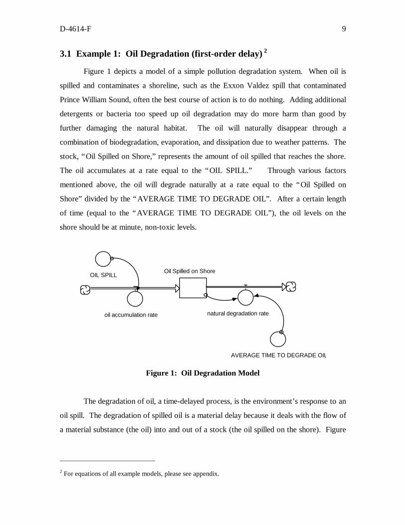
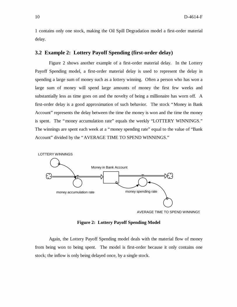
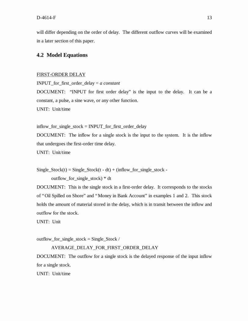
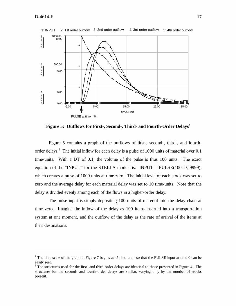
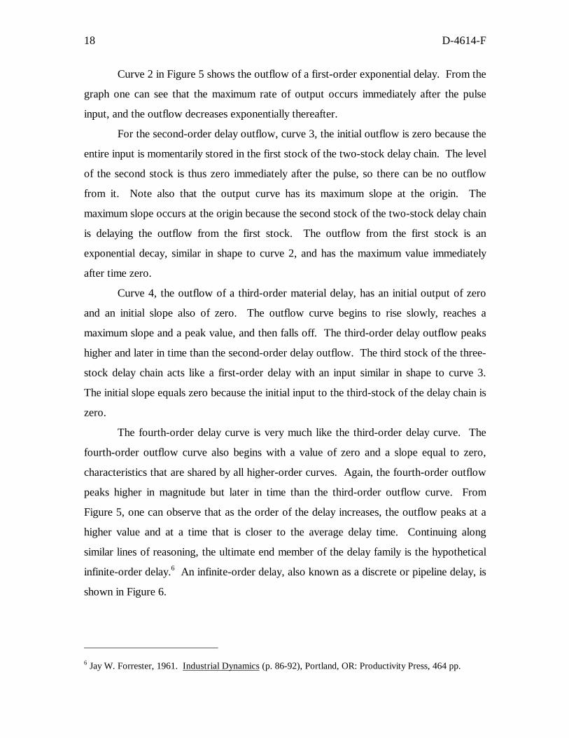
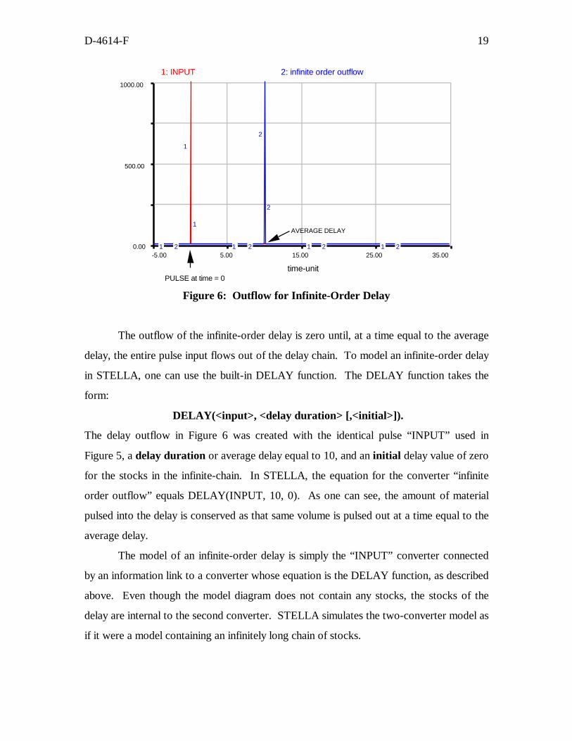
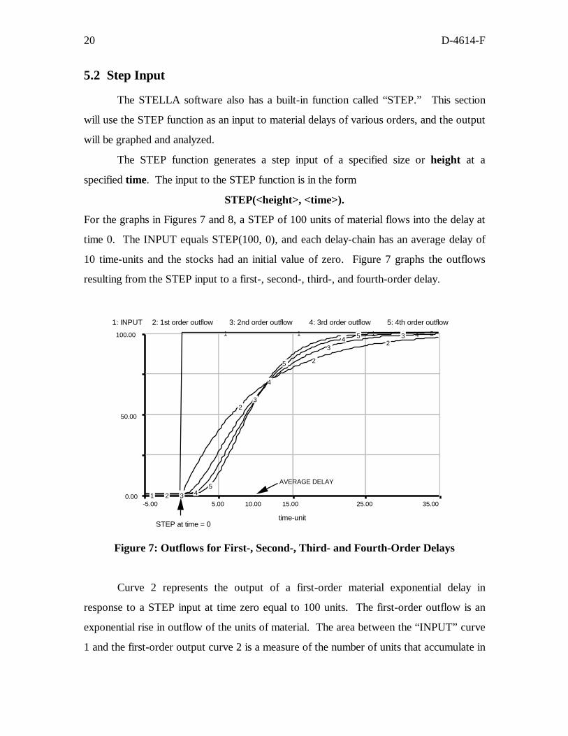
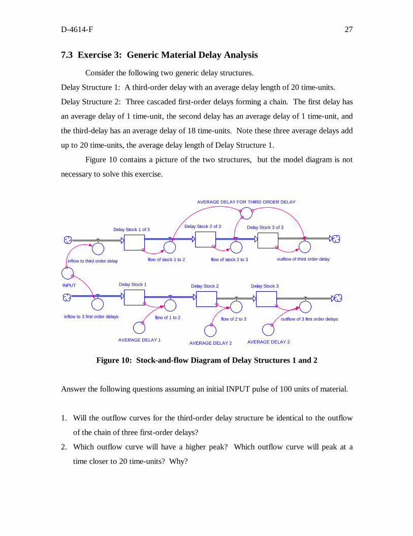
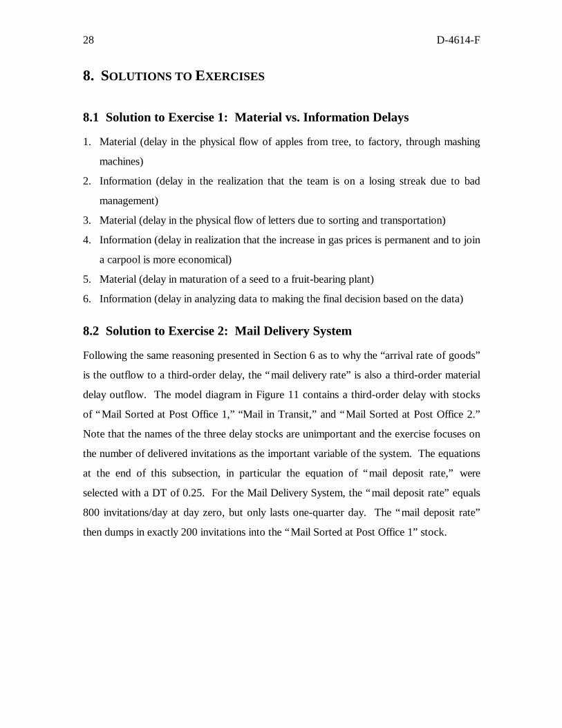
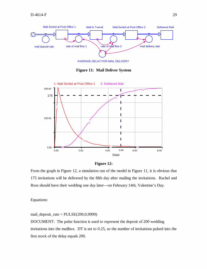
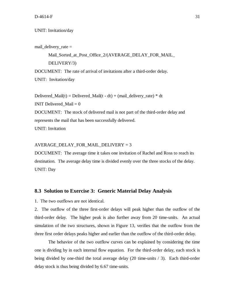
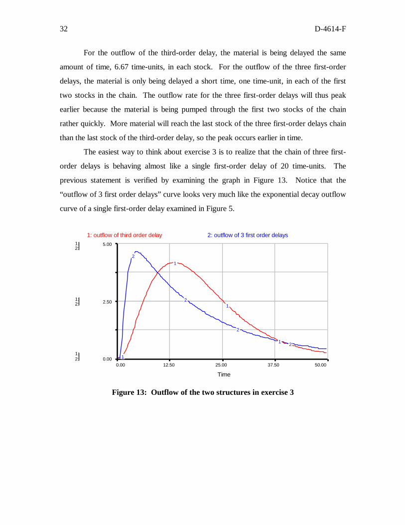