Delft University of Technology

Generic EMT Model for Real-Time Simulation of Large Disturbances in 2 GW OffshoreHVAC-HVDC Renewable Energy Hubs

Ganesh, Saran ; Perilla , Arcadio; Rueda Torres, Jose ; Palensky, Peter; Lekic, Aleksandra; van derMeijden, MartDOI10.3390/en14030757Publication date2021Document VersionFinal published versionPublished inEnergies

Citation (APA)Ganesh, S., Perilla , A., Rueda Torres, J., Palensky, P., Lekic, A., & van der Meijden, M. (2021). GenericEMT Model for Real-Time Simulation of Large Disturbances in 2 GW Offshore HVAC-HVDC RenewableEnergy Hubs. Energies, 14(3), 1-30. [757]. https://doi.org/10.3390/en14030757

Important noteTo cite this publication, please use the final published version (if applicable).Please check the document version above.

CopyrightOther than for strictly personal use, it is not permitted to download, forward or distribute the text or part of it, without the consentof the author(s) and/or copyright holder(s), unless the work is under an open content license such as Creative Commons.

Takedown policyPlease contact us and provide details if you believe this document breaches copyrights.We will remove access to the work immediately and investigate your claim.

This work is downloaded from Delft University of Technology.For technical reasons the number of authors shown on this cover page is limited to a maximum of 10.

energies

Article

Generic EMT Model for Real-Time Simulation of LargeDisturbances in 2 GW Offshore HVAC-HVDC RenewableEnergy Hubs

Saran Ganesh 1, Arcadio Perilla 1 , Jose Rueda Torres 1,* , Peter Palensky 1 , Aleksandra Lekic 1

and Mart van der Meijden 1,2

�����������������

Citation: Ganesh, S.; Perilla, A.;

Rueda Torres, J.; Palensky, P.; Lekic,

A.; van der Meijden, M. Generic EMT

Model for Real-Time Simulation of

Large Disturbances in 2 GW Offshore

HVAC-HVDC Renewable Energy

Hubs. Energies 2021, 14, 757. https://

doi.org/10.3390/en14030757

Academic Editor: Georgios Konstantinou

Received: 30 November 2020

Accepted: 22 January 2021

Published: 1 February 2021

Publisher’s Note: MDPI stays neutral

with regard to jurisdictional claims in

published maps and institutional

affiliations.

Copyright: © 2021 by the authors.

Licensee MDPI, Basel, Switzerland.

This article is an open access article

distributed under the terms and

conditions of the Creative Commons

Attribution (CC BY) license (https://

creativecommons.org/licenses/by/

4.0/).

1 Department of Electrical Sustainable Energy, Delft University of Technology, Mekelweg 4,2628 CD Delft, The Netherlands; S.GANESH-2@student.tudelft.nl (S.G.); A.Perilla@tudelft.nl (A.P.);P.Palensky@tudelft.nl (P.P.); A.Lekic@tudelft.nl (A.L.); Mart.vander.Meijden@tennet.eu (M.v.d.M.)

2 TenneT TSO B.V., 6812 AR Arnhem, The Netherlands* Correspondence: J.L.RuedaTorres@tudelft.nl

Abstract: This paper proposes a Electro-Magnetic Transient (EMT) model of a 2 GW offshore networkwith the parallel operation of two Modular Multi-level Converter (MMC)—High Voltage DirectCurrent (HVDC) transmission links connecting four Offshore Wind Farms (OWFs) to two onshoresystems, which represent a large scale power system. Additionally, to mitigate the challenges corre-sponding to voltage and frequency stability issues in large scale offshore networks, a Direct VoltageControl (DVC) strategy is implemented for the Type-4 Wind Generators (WGs), which representthe OWFs in this work. The electrical power system is developed in the power system simulationsoftware RSCADTM, that is suitable for performing EMT based simulations. The EMT model of2 GW offshore network with DVC in Type-4 WGs is successfully designed and it is well-coordinatedbetween the control structures in MMCs and WGs.

Keywords: large scale offshore network; direct voltage control; EMT; MMC; HVDC

1. Introduction

According to the Paris Agreement, the European Union’s (EU) should contribute inreduction of greenhouse gas emissions by at least 40% by 2030 when compared to 1990 [1].The plans involve a future target between 70 GW to 150 GW offshore wind power installedin the North Sea by 2040. The latest European Commission prediction estimates installationof 140 to 450 GW offshore wind power in the EU by 2050. With the current pace, the rateof offshore wind energy deployment is deficient in comparison to the Paris Agreementobjectives [1]. To comply with these objectives, an extraordinary jump in offshore windenergy is required. A practical solution calls for an increase in large scale offshore windenergy deployment in the North Sea [2]. As the part of the North Sea Wind Power HubProgramme [3], the Transmission System Operator (TSO) of the Netherlands, TenneT, hasalready entered into an innovation partnership with its suppliers to establish a 2 GWoffshore platform. Likewise, Denmark is progressing with the first hub-and-spoke energyisland with a vision of connecting at least 10 GW of offshore wind power in the NorthSea [4].

Currently, the state-of-the-art technology for the transfer of offshore wind power tothe onshore system are Voltage Source Converter (VSC) based-HVDC transmission links.Presently, MMC topology, that falls under the classification of VSC topologies, is the mostsuitable solution. Advantages of the MMC are [5]: (1) ease of integration with OWFs, (2) sup-port of the bi-directional power flow between the offshore network and onshore system, and(3) independent control of active and reactive powers in the network. However, with theavailable technology, MMC-HVDC transmission are limited to a rated capacity of 1.2 GW [6].

Energies 2021, 14, 757. https://doi.org/10.3390/en14030757 https://www.mdpi.com/journal/energies

Energies 2021, 14, 757 2 of 30

The implementation of large scale offshore networks (greater than or equal to 2 GW)creates a highly Power Electronic (PE) converter dominated network. The absence ofconventional generators would mean that the PE converters will have to take into accountthe decreasing inertia of the system that leads to faster dynamic behaviour, and it requirescontrollers with shorter time response. The challenges in design of PE converters’ voltageand frequency controls, without conventional units, are prominent in large scale offshorenetworks. Moreover, distant OWFs would be connected in parallel. With the paralleloperation of the conventional current controllers in WGs, interactions can persist amongthem and could lead to instability of the network. Additionally, the restoration of the grid,following disturbances by the PE converter units, is a serious matter of concern. With theconventional current control approach, grid restoration is challenging without the helpof auxiliary diesel generators. However, in the case of large scale offshore networks, PEconverters take the role of grid restoration. There can be arguments that storage facilitiessuch as battery and thermal can be a realizable solution in case when there are no conven-tional generators available. Huge investment costs, low lifetime and low efficiency whencompared to controller modifications are the drawbacks that make these storage facilitiespractically unusable in large scale offshore networks [7].

Conventionally, the OWFs are coupled to an AC collector platform through 33 kVHigh Voltage Alternating Current (HVAC) cables. The voltage is stepped-up to 145 kVusing a power transformer at the collector platform, and power is transferred to the offshoreconverter station using 145 kV HVAC cables. However, in the upcoming projects, the ratedvoltage levels are expected to increase from 33 kV to 66 kV to avoid the use of a collectorplatform and to directly transfer power from OWFs to the offshore converter station using66 kV HVAC cables. Hence, it is necessary understand the performance of large scaleoffshore networks developed with 66 kV voltage rating.

With the available MMC-HVDC transmission technology, multiple MMC-HVDCtransmission links connected in parallel would be required to transfer the bulk amount ofoffshore wind power generated from large scale offshore networks to the onshore system.The power flow between the parallel operated MMCs and the OWFs must be coordinatedboth during steady state and dynamic conditions. The major challenges regarding voltageand frequency control during islanding of the OWFs must be taken into account. Thescenario of reactive current injection that needs to be provided by the WGs during dynamicconditions must also be taken into consideration [8]. Therefore, the progress towards thedevelopment of large scale offshore networks calls for a generic model with a suitablelayout and available technology that is capable of tackling the aforementioned technicalchallenges and providing stable operation during steady state and dynamic conditions.

This paper adopts the latest trend in technology, and achieves the overall goal ofdeveloping a generic EMT model of 2 GW, 66 kV HVAC offshore network in RSCAD. Theperformance of the model is analyzed based on the voltage and active power values atvarious locations in the network for highly severe dynamic conditions. The EMT modeldeveloped in this paper adopts a modified layout with two MMCs working in parallel andconnecting four OWFs to the onshore system. The layout of the 2 GW offshore network isachieved using hub-and-spoke principle from [9] which involves connecting an offshore“hub” to several onshore grids in same or different areas through “spokes”. Additionally,the technical challenges faced while using conventional current control strategies in WGs,related to voltage and frequency control, are mitigated by implementing DVC from [10] inall Type-4 WGs in RSCAD for real-time application. The novelty of the paper lies in theimplementation of DVC in four WGs in parallel operation and work in coordination withtwo MMCs with different control strategies during steady-state and dynamic conditions inthe network.

The sections of the paper are arranged as follows. In Section 2, the processors availablefor modelling in RSCAD are described. Furthermore, it is given the topology selected forthe 2 GW offshore network. Section 3 describes the model layout of the 2 GW offshorenetwork. The control structures utilized in the 2 GW offshore network are discussed in

Energies 2021, 14, 757 3 of 30

Section 4. Section 5 depicts preset conditions before the start of the simulation of the model,the synchronization of the offshore converter stations, and the energization of the HVACcables and OWFs. It also employs the dynamic performance analysis for the 2 GW EMTmodel. Section 6 concludes the paper.

2. Defining the Layout for the 2 GW Offshore Network

The initial aspect of an offshore network is the topology of the network. The MMC,due to its improved controllability and superior system performances, has been oftenemployed for MMC-HVDC transmission for integration of the distant OWFs. For theconnection of new OWFs in the vicinity of the already existing ones, parallel operation ofMMC-HVDC transmission systems can be constructed. It is expected that in the near futurewill be used parallel MMC-HVDC to create multiple connections to the onshore system.Thus, the interest in hybrid systems with the hub-and-spoke principle proposed by ABB [9]has been increased. It is represented in Figure 1. In the Figure 1a is depicted connection ofOWFs to an offshore converter station, which in turn transfers power to the onshore systemthrough multi-terminal HVDC connections. However, the scaling of offshore wind poweris limited to the installed capacity of MMC unit in such a layout. Another layout involvesthe OWFs connected through AC links to a back-to-back HVDC converter station as shownin Figure 1b. Long distance HVAC transmission is required for the transfer of power fromOWFs to the onshore network, and hence, it contributes to high losses in the network whencompared to HVDC transmission for larger distances. Figure 1c represents the connectionof multiple OWFs to the offshore converter station, where the power is transferred to theonshore system through multiple HVDC links. This layout provides contingency in thenetwork by supplying offshore wind power to at least one onshore system if one of theHVDC links gets disconnected [11]. A stage-wise construction of such a HVDC project iseasier to be achieved by the developers as well [5].

A specific configuration for a 2 GW offshore network is currently non-existent, andthis paper tries to fill this research gap. This paper expands the single OWF model from [12]to create 2 GW offshore wind power network. This is possible by connecting four OWFmodels, each generating power of ∼500 MW, in parallel. The reason for choosing fourOWFs is to ensure a symmetrical layout and to test the ability of RSCAD to perform simu-lations on such configuration. Correspondingly, a 2 GW offshore converter station capacityis required to transfer the generated amount of power to the onshore system. However,currently deployed (state-of-the-art) MMC-HVDC transmission, has a maximum ratedcapacity of 1.2 GW [6]. Hence, with the available technology, two MMC offshore stationsof 1 GW each will be required for 2 GW power transmission. Taking the aforementionedfactors into account, a modified layout of Figure 1c is developed for this work.

2.1. Scaling of Single OWF Model for 2 GW Offshore Network

The 2 GW offshore network is modelled using RSCAD simulation tool which runs onReal Time Digital Simulator (RTDS) clusters. RSCAD simulations can be run either usingNovaCor or PB5 processor cards. For this workd is chosen NovaCor processor, because ithas 2–3 times higher simulation capacity than completely loaded PB5 processor [13]. For anextensive power system network, NovaCor processor requires distribution of the systeminto subsystems. RSCAD allows provision for splitting of the network into subsystems ifthe network is large. This feature is utilized using Tline modules, that are used to connectsubsystems, which is explained in Section 3.2 in detail.

There are two NovaCor processors available at TU Delft, and they are equipped withfour cores each. These cores are utilized to solve the overall network solution, auxiliarycomponents (such as transformers, cables, generators etc.) and the controls present inthe simulation. Assignment of cores for solving various components of the network is animportant step that needs to be considered while modelling, as they depict the total loadthat is distributed over the available cores. The process is detailed in Section 3.1.

Energies 2021, 14, 757 4 of 30

Onshore grid

A

Onshore grid

B

Offshore

(a)

Onshore grid

A

Onshore grid

B

Offshore

(b)

Onshore grid

A

Onshore grid

B

Offshore

(c)

Figure 1. Different configurations available for Hub-and-spoke principle. (a) Hub-and-spoke withmulti-terminal HVDC system; (b) Hub-and-spoke with AC links and HVDC back-to-back station;(c) Hub-and-spoke with multiple HVDC links.

The layout of the 2 GW offshore network is built in RSCAD by scaling aggregatedOWF model from [12]. A modular topology is considered to achieve the capacity of 2 GW.The following steps are utilized:

• The aggregated OWF model in [12] provides a generation of ∼700 MW. The first stepinvolves reducing this generation to ∼500 MW, because there are four planned OWFs.This is achieved by reducing the number of parallel WG units from 116 (116 × 6 MW= 696 MW) to 83 (83 × 6 MW = 498 MW), which is done by changing the scaling factor

Energies 2021, 14, 757 5 of 30

at the OWF transformer. Thus, OWF generates approximately ∼500 MW, as shown inFigure 2.

• The second step involves the connection of two OWFs in parallel to the external ACsystem in a modular approach. This allows for the generation of 1 GW of power,as depicted in Figure 3. All control structures incorporated in OWF-1 are replicatedfor OWF-2.

• In the third step, the external AC system is replaced by an offshore converter station,consisting of the average EMT model of MMC (MMC-1) and the interface transformer(IT-1), which is available in the CIGRE B4 DC Grid Test System [14]. The same isdepicted in Figure 4. As the final layout network would be extensive, it is required tosplit the network into subsystems. The splitting into two subsystems is performed inthis step. The offshore converter station is modelled in subsystem-1, and the OWFsare modelled in subsystem-2. MMC-1 is designed to operate in V/F control (or gridforming control), which is explained at the end of this section.

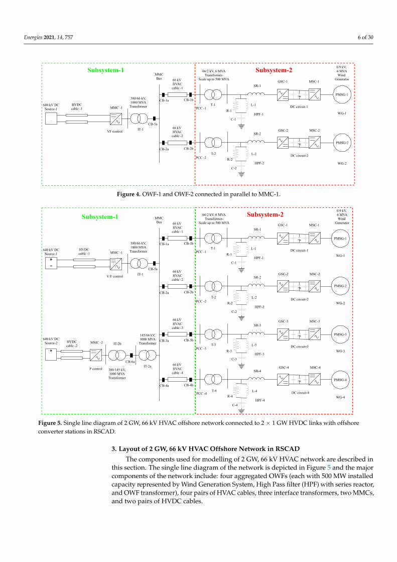
• The final step involves parallel connection of the two more OWF models (OWF-3 andOWF-4), generating ∼500 MW each, using modular approach. Additionally, anotheroffshore converter station, consisting of a similar average EMT model of MMC (MMC-2) and two interface transformers (IT-2a and IT-2b), is connected in parallel to theprevious converter station. The need for two interface transformers in MMC-2 bus isexplained in the following sections of the paper. Therefore, the final layout shown inFigure 5 represents a total of 2 GW offshore wind power transmission.

T-1

0.9kV,6MVAWind

GeneratorMSC-1GSC-1SR-1

66/2kV,6MVA

Transformer-Scaleupto500MVA66kV

HVACcable-1

ExternalACsystem

DCcircuit-1R-1

L-1

C-1

WG-1

PMSG-1

OWF-1

MMCBus

PCC-1

HPF-1

CB-1bCB-1a

Figure 2. OWF-1 connected to external AC system.

0.9kV,6MVAWind

Generator

R-2

R-1

CB-2bCB-2a

CB-1bCB-1a

SR-1

HPF-1

66/2kV,6MVATransformer-

Scaleupto500MVAMMCBus 66kV

HVACcable-1

WG-1L-1

C-1

MSC-1GSC-1

DCcircuit-1

66kVHVACcable-2

WG-2

T-1

SR-2

HPF-2

L-2

C-2

MSC-2GSC-2

DCcircuit-2T-2PCC-2

PCC-1

PMSG-1

PMSG-2

ExternalACsystem

Figure 3. OWF-1 and OWF-2 connected in parallel to external AC system.

Energies 2021, 14, 757 6 of 30

0.9kV,6MVAWind

Generator

R-2

R-1

CB-2bCB-2a

CB-1bCB-1a

SR-1

HPF-1

66/2kV,6MVATransformer-

Scaleupto500MVAMMCBus 66kV

HVACcable-1

WG-1

L-1

C-1

MSC-1GSC-1

DCcircuit-1

66kVHVACcable-2

WG-2

T-1

SR-2

HPF-2

L-2

C-2

MSC-2GSC-2

DCcircuit-2T-2PCC-2

PCC-1

Subsystem-1 Subsystem-2

PMSG-1

PMSG-2

380/66kV,1000MVATransformerMMC-1

HVDCcable-1

640kVDCSource-1

VFcontrol IT-1CB-5a

Figure 4. OWF-1 and OWF-2 connected in parallel to MMC-1.

CB-6a

0.9kV,6MVAWind

Generator

R-2

R-3

R-4

R-1

CB-4bCB-4a

145/66kV,1000MVATransformer

CB-3bCB-3a

CB-2bCB-2a

CB-1bCB-1a

380/145kV,1000MVATransformer

SR-1

HPF-1

66/2kV,6MVATransformer-

Scaleupto500MVAMMCBus

380/66kV,1000MVATransformerMMC-1

66kVHVACcable-1

HVDCcable-1

640kVDCSource-1

V/Fcontrol

Pcontrol

MMC-2HVDCcable-2

WG-1

640kVDCSource-2

L-1

C-1

MSC-1GSC-1

DCcircuit-1

66kVHVACcable-2

WG-2

66kVHVACcable-3

WG-3

66kVHVACcable-4

WG-4

T-1

SR-2

HPF-2

L-2

C-2

MSC-2GSC-2

DCcircuit-2T-2

SR-3

HPF-3

L-3

C-3

MSC-3GSC-3

DCcircuit-3T-3

SR-4

HPF-4

L-4

C-4

MSC-4GSC-4

DCcircuit-4T-4PCC-4

PCC-3

PCC-2

PCC-1

IT-1

IT-2a

IT-2b

Subsystem-1 Subsystem-2

PMSG-1

PMSG-2

PMSG-3

PMSG-4

CB-5a

Figure 5. Single line diagram of 2 GW, 66 kV HVAC offshore network connected to 2 × 1 GW HVDC links with offshoreconverter stations in RSCAD.

3. Layout of 2 GW, 66 kV HVAC Offshore Network in RSCAD

The components used for modelling of 2 GW, 66 kV HVAC network are described inthis section. The single line diagram of the network is depicted in Figure 5 and the majorcomponents of the network include: four aggregated OWFs (each with 500 MW installedcapacity represented by Wind Generation System, High Pass filter (HPF) with series reactor,and OWF transformer), four pairs of HVAC cables, three interface transformers, two MMCs,and two pairs of HVDC cables.

Energies 2021, 14, 757 7 of 30

3.1. Aggregated OWF

As mentioned in Section 2.1, the 2 GW offshore wind power is split into four OWFs,with approximately 500 MW rated capacity each. Currently, the largest offshore WGdeveloped by GE Renewable Energy has a rating of 12 MW [15]. The standard model fora Type-4 WG in RSCAD is rated 6 MW. Hence, to represent a 500 MW OWF, 83 WGs arerequired. All OWFs are at a distance of 30 km from the MMC bus.

The average RSCAD model of Type-4 WG is used. The aggregated OWF modelrepresented in a small time step environment described in [12] is used here for all thefour OWFs. As the entire network is extensive, it is split into two subsystems in RSCAD,as shown in Figure 5. The four OWFs are modelled in subsystem-2, and the rest of thesystem is modelled in subsystem-1. Each subsystem requires one rack for operation, andhence two NovaCor racks are used. It is also possible to simulate the network with PB5processor. However, this requires three subsystems, since PB5 racks allow only smallnetwork simulation [16]. Therefore, two OWFs are to be modelled in subsystem-3, othertwo OWFs in subsystem-2 and the rest of the network in subsystem-1. Henceforth, thesimulations are implemented only on NovaCor processor. Since there is a need for fourdifferent small time step blocks which represent four OWFs, each block needs to be setwith different step sizes to avoid conflict during initialization. Moreover, if the time stepsare not initialized properly, it could lead to the occurrence of a time step overflow errorduring the simulation in the Runtime module.

Another essential parameter to be considered here is the assignment of the coresfor the small time step blocks. NovaCor processor at TU Delft has four cores, and eachcomponent used in the network can be assigned to specific core (1 to 4 in number). Sincethere are six small time step blocks (OWF-1, 2, 3 and 4; MMC-1 and MMC-2), the coresneed to be manually assigned to each block to allocate the load on each processor withintheir capacity. The core allocation of the small time step blocks representing OWFs for thisnetwork is chosen, as shown in Table 1.

Table 1. Core assignment of OWF models in subsystem-2.

Small Time Step Block Core Assignment

OWF-1 4OWF-2 1OWF-3 3OWF-4 1

3.2. HVAC Cables

The HVAC cables transfer power from the OWFs to the offshore converter stations.Hence, four pairs of HVAC cables are required to transfer power from four OWFs. Thecables are rated at 66 kV and are 30 km long. In the RSCAD network layout, as shown inFigure 5, the HVAC cables connect OWFs in subsystem-1 with the MMC bus in subsystem-2. To provide connection between components placed in different subsystems in RSCAD, afeature called Tline module is used.

The cables are modelled as Bergeron models with RLC data parameters. Bergeronmodel is chosen to test the working of the network using travelling wave model. Moreover,as the 2 GW offshore network is developed from the single OWF model in [12], the sameRLC cable parameters used in [12] are used in the Tline module for all four pairs of cables.

3.3. Offshore Converter Stations

The offshore converter stations convert HVAC offshore wind power to HVDC totransfer the power to the onshore system through HVDC links. The existing availableHVDC links in the industry have a rated capacity of 1.4 GW. Examples of these projectsare the NordLink cable connecting Norway and Denmark, NSN Link connecting Norwayand the United Kingdom [17]. Moreover, the standard EMT models for MMCs available

Energies 2021, 14, 757 8 of 30

in CIGRE B4 DC Grid Test System [14] have a rated capacity of 1.2 GW. Therefore, withthe currently available technology, two offshore converter stations are required for thetransfer of 2 GW offshore wind power. As MMCs also involve PE components, similarto the OWF model, the average EMT model of MMC is also represented in a small timestep environment in RSCAD, in order to represent fast switching events accurately. Theaverage EMT model consists of the MMC and interface transformer modelled in the smalltime step environment, which represents the offshore converter station. For this work, twosmall time step blocks are required for the representation of two offshore converter stations.Both blocks are placed in subsystem-1. Again, these two blocks need to be initializedwith different time step to avoid conflict during initialization and thereby, avoiding thetime step overflow error during the start of simulation. To evenly distribute the load onfour cores, considering the core allocation for OWFs in Table 1, the cores for MMCs areallocated as shown in Table 2. The offshore converter station-1 consists of the interfacetransformer (IT-1) and MMC-1 whereas offshore converter station-2 consists of the interfacetransformers (IT-2a, IT-2b) and MMC-2.

Table 2. Core assignment of MMC models in subsystem-1.

Small Time Step Block Core Assignment

MMC-1 3MMC-2 2

3.3.1. Interface Transformers

Interface transformers (also termed as converter transformers) are connected to theAC side of MMCs and depicted as IT-1 for offshore converter station-1 and IT-2a and IT-2bfor offshore converter station-2, see Figure 5. As explained in [18], these transformersprovide reactance between the offshore network and the MMC, and prevent the flow ofzero sequence currents between the offshore network and the MMC.

As mentioned in Section 3.3, in the available average EMT models in RSCAD library,the interface transformer is modelled with the MMC in a small time step environment.Considering a delta-wye type interface transformer and connecting MMC to the deltaside of the transformer, allows isolation of the zero sequence currents during faults. Theavailable EMT models for offshore MMC stations from [14] are utilized in this work. Thesemodels are designed for 145 kV HVAC offshore network. Hence, the secondary side voltageof the transformer is changed from 145 kV to 66 kV. Additionally, there were modificationsin the control structures of the MMC to make them fitting for the 66 kV HVAC network.Control modifications are explained in the next section.

There are mainly three interface transformers used in this work. The transformer(IT-1) is rated 66/380 kV, 1000 MVA in the offshore converter station-1. Two interfacetransformers in the offshore converter station-2 are rated 66/145 kV, 1000 MVA (IT-2a) and145/380 kV, 1000 MVA (IT-2b) respectively. The need for two interface transformers inoffshore converter station-2 is explained in the later sections in the paper.

3.3.2. Modular Multilevel Converters (MMCs)

The average EMT model of MMC in RSCAD has the option of modelling the MMCusing half-bridge submodules or full-bridge submodules [19]. The voltage levels for HVDCoffshore wind farm projects in Europe range from 300 kV to 640 kV DC voltage [17]. Hence,to continue with the latest trend, a voltage level of 640 kV DC is chosen for this work.Therefore, 320 submodules are required per arm to create a voltage of ±320 kV for thepositive and negative poles, respectively. Both MMCs (MMC-1 and MMC-2) in the offshoreconverter stations are modelled for 640 kV DC.

Energies 2021, 14, 757 9 of 30

3.4. HVDC Cables

The HVDC cables transfer the generated wind power from the offshore converterstation to the onshore system. As mentioned in the section above, the voltage level chosenfor HVDC transmission in this work is 640 kV DC. Therefore, each cable model mustbe suitable for ±320 kV. The cable parameters available in [14] designed for ±400 kVvoltage are utilized in this work. The cable model is represented in frequency-dependentphase domain using the Cable module available in RSCAD. The cables are modelled insubsystem-1 and labelled as HVDC cable-1,2 for the connection from offshore converterstation-1 and offshore converter station-2 to the onshore system, respectively (see Figure 5).

3.5. Onshore Equivalent Converter Stations

The connection between offshore converter station and the onshore converter stationfollows a symmetrical monopole configuration, as shown in Figure 6a [20]. The DC partof the onshore converter stations are simplified and represented using an equivalent DCsource, as shown in Figure 6b. This simplification is valid, because the paper deals withdynamical performance on the network’s AC side. Conventionally, the onshore converterstations provide DC voltage and reactive power control. Hence, the representation of aconstant DC voltage source ensures the DC voltage control during the time of disturbancesin the AC offshore network. The voltages of the DC sources are 640 kV.

Offshoreconverterstation

Onshoreconverterstation HVDCcable

(a)

DCsource

Offshoreconverterstation

Onshoreequivalentconverterstation HVDCcable

(b)

Figure 6. Symmetrical monopole configuration in HVDC network. (a) Symmetrical monopoleconfiguration; (b) Symmetrical monopole configuration by equivalent representation of DC side ofonshore MMC station using a constant DC source.

4. Control Structures

This section explains the different control structures and the modifications required toensure converters’ operation in the 66 kV HVAC network. The DVC from [21] for Type-4WG, firstly implemented in [12], is extended for the 2 GW offshore network. There arethree control strategies used: DVC in the GSCs of the WGs used to represent aggregatedOWFs, island mode control in MMC-1, and non- island mode control in MMC-2.

4.1. DVC

The control structure explained in [12] is implemented for all the four WGs. Since thesame type of model is used for GSCs in all four WGs, the control loop parameters remainthe same.

4.2. Island Mode Control

It is highly necessary to use a control strategy in any of the MMCs which couldprovide the voltage and frequency reference for the MMC bus since it is connected to aweak network (OWF network). The reference voltage is created by the V/F control mode,

Energies 2021, 14, 757 10 of 30

which comes under the classification of the islanded mode of control for VSCs [14]. Forthis study, MMC-1 is operated in the V/F control. A basic control strategy was developedaccording to the illustration provided in [22] and it is shown in Figure 7. Since the voltageangle reference (θ) is generated by an independent Voltage Controlled Oscillator (VCO),this control is termed under island mode operation. Such an approach provides the gridforming behaviour for MMC-1, which is responsible for providing and absorbing powerfrom the OWF network when required. With this control the power flow is kept in balanceduring the steady state and transient conditions [5].

The V/F control consists of a PI controller whose input is the difference betweenthe measured voltage (VPCC) and the reference PCC voltage (VPCC_re f ), given in p.u. PIcontroller provides a reference d-axis converter voltage (VPCC_d) that is translated to abcframe (Vabc_re f ), as shown in Figure 7. This makes VPCC_d to be aligned with the gridvoltage and the q-axis voltage (VPCC_q) is set to zero. The parameters for the PI gainsused for this control are referred from [14]. It should be noted that all figures representingcontrol approach have notation in Laplace domain, where s is a Laplace operator.

+-

𝑉𝑃𝐶𝐶

𝑉𝑃𝐶𝐶_𝑟𝑒𝑓

𝑉𝑚𝑎𝑥

𝑉𝑎𝑏𝑐_𝑟𝑒𝑓𝑉𝑚𝑖𝑛

θ50 𝐻𝑧

𝑉𝑃𝐶𝐶_𝑑𝑘𝑝_𝑣𝑓 +

𝑘𝑖_𝑣𝑓

𝑠

0

2𝜋

𝑅𝑎𝑚𝑝

𝑑𝑞0

𝑎𝑏𝑐𝑉𝑃𝐶𝐶_𝑞 = 0

Figure 7. V/F control in MMC-1.

4.3. Non-Island Mode Control

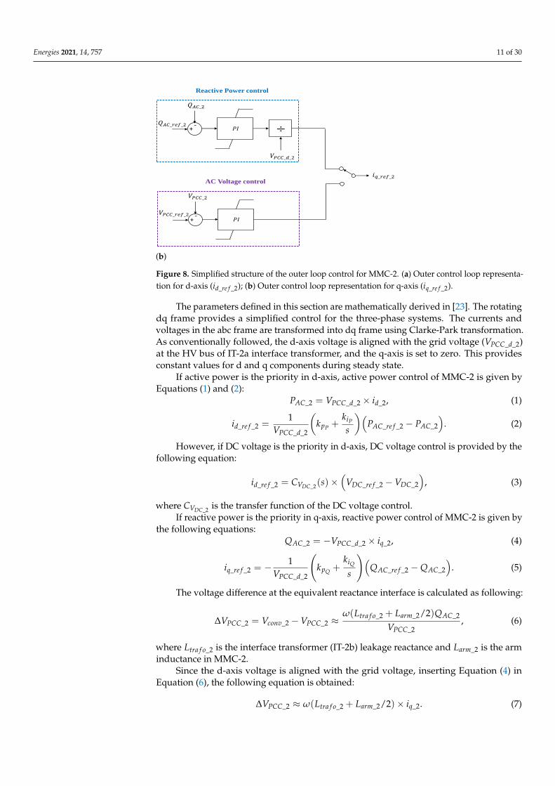
This mode of operation is based on the conventional current control (grid following)approach, which consists of the outer control loop and the inner control loop. The outerloop consists of the direct (d) and quadrature (q) axes loops. The d-axis loop can providecontrol of DC voltage or active power and the q-axis loop can provide control of an ACvoltage or reactive power, as depicted in Figure 8a and Figure 8b, respectively. The outercontrol loop provides the respective current reference values as inputs for the inner currentloops. MMC-2 is configured with this control for this work.

𝑃𝐼+-

𝑃𝐴𝐶_2

𝑃𝐴𝐶_𝑟𝑒𝑓_2

Active Power control

𝑉𝑃𝐶𝐶_𝑑_2

𝑃𝐼+-

𝑉𝐷𝐶_2

𝑉𝐷𝐶_𝑟𝑒𝑓_2

DC Voltage control𝑖𝑑_𝑟𝑒𝑓_2

÷

(a)

Figure 8. Cont.

Energies 2021, 14, 757 11 of 30

𝑃𝐼+-

𝑄𝐴𝐶_2

𝑄𝐴𝐶_𝑟𝑒𝑓_2

Reactive Power control

÷

𝑉𝑃𝐶𝐶_𝑑_2

𝑃𝐼+-

𝑉𝑃𝐶𝐶_2

𝑉𝑃𝐶𝐶_𝑟𝑒𝑓_2

AC Voltage control𝑖𝑞_𝑟𝑒𝑓_2

(b)

Figure 8. Simplified structure of the outer loop control for MMC-2. (a) Outer control loop representa-tion for d-axis (id_re f _2); (b) Outer control loop representation for q-axis (iq_re f _2).

The parameters defined in this section are mathematically derived in [23]. The rotatingdq frame provides a simplified control for the three-phase systems. The currents andvoltages in the abc frame are transformed into dq frame using Clarke-Park transformation.As conventionally followed, the d-axis voltage is aligned with the grid voltage (VPCC_d_2)at the HV bus of IT-2a interface transformer, and the q-axis is set to zero. This providesconstant values for d and q components during steady state.

If active power is the priority in d-axis, active power control of MMC-2 is given byEquations (1) and (2):

PAC_2 = VPCC_d_2 × id_2, (1)

id_re f _2 =1

VPCC_d_2

(kpP +

kiP

s

)(PAC_re f _2 − PAC_2

). (2)

However, if DC voltage is the priority in d-axis, DC voltage control is provided by thefollowing equation:

id_re f _2 = CVDC_2(s)×(

VDC_re f _2 −VDC_2

), (3)

where CVDC_2 is the transfer function of the DC voltage control.If reactive power is the priority in q-axis, reactive power control of MMC-2 is given by

the following equations:QAC_2 = −VPCC_d_2 × iq_2, (4)

iq_re f _2 = − 1VPCC_d_2

(kpQ +

kiQ

s

)(QAC_re f _2 −QAC_2

). (5)

The voltage difference at the equivalent reactance interface is calculated as following:

∆VPCC_2 = Vconv_2 −VPCC_2 ≈ω(Ltra f o_2 + Larm_2/2)QAC_2

VPCC_2, (6)

where Ltra f o_2 is the interface transformer (IT-2b) leakage reactance and Larm_2 is the arminductance in MMC-2.

Since the d-axis voltage is aligned with the grid voltage, inserting Equation (4) inEquation (6), the following equation is obtained:

∆VPCC_2 ≈ ω(Ltra f o_2 + Larm_2/2)× iq_2. (7)

Energies 2021, 14, 757 12 of 30

The control of AC voltage is obtained with the following equation:

iq_re f _2 =

(kpV +

kiVs

)(VPCC_re f _2 −VPCC_2

). (8)

The inner loop consists of PI controllers for d and q axis separately, and it provides adecoupled control action. The output from the inner control loop control is then translatedback to the abc frame using dq to abc frame transformation.

As the DC voltage in the HVDC link is maintained and controlled by the onshoreequivalent MMC station represented by a constant DC source, the active power control ischosen as priority for d-axis for MMC-2 control. Similarly, as the AC voltage is controlledby the V/F control in MMC-1, reactive power control is chosen as priority chosen forq-axis for MMC-2. When active power is the chosen priority, PAC_re f _2 represents therequired amount of active power that must flow through offshore converter station-2 andmust be defined externally by the user. However, the outer loop control available for thenon-islanded mode in [14] is not suitable for parallel operation with V/F control. Hence,the outer loop is simplified, and the reference points id_re f _2 and iq_re f _2 for the inner loopare controlled directly by the user. The inner control loop consists of PI controllers that playthe major role in ensuring minimum steady state error. The inner control also contains thefeed-forward term to compensate the cross coupling terms. The mathematical equations forthe parameters of inner control loop are derived as provided in [23]. Applying Kirchoff’sVoltage Law in Figure 9 and with the MMC representation in Figure 10, the equations arederived for offshore converter station-2 connected to the AC network. The assumptionsinvolve, the direction of current is from the AC network to the MMC (the condition whenoffshore wind power is transferred from the offshore network to onshore system) andavoiding the star-point reactor:

VDC_2

2= vuj + Larm_2

diuj

dt+ Rarm_2iuj − Ltra f o_2

dij

dt− Rtra f o_2ij + vPCCj , (9)

VDC_2

2= vl j + Larm_2

dil jdt

+ Rarm_2il j + Ltra f o_2dij

dt+ Rtra f o_2ij − vPCCj , (10)

where Rtra f o_2 is the interface transformer (IT-2b) resistance, Rarm_2 is the equivalent armresistance in MMC-2, vPCCj is the voltage at HV bus of IT-2a, j ∈ {a, b, c} represents phases.Upper arm and lower arm of the MMC-2 are denoted as u and l, respectively.

HV bus of IT-2a

Sta

rt-p

oin

t re

acto

r AC breaker

MMC-2

Interface

transformer

IT-2b

Figure 9. Representation of offshore converter station-2 connection to the AC offshore network.

Energies 2021, 14, 757 13 of 30

𝑆𝑀1𝑢𝑐

𝑆𝑀2𝑢𝑐

𝑆𝑀𝑁𝑢𝑐

𝑆𝑀1𝑢𝑏

𝑆𝑀2𝑢𝑏

𝑆𝑀𝑁𝑢𝑏 𝑆𝑀𝑁𝑢𝑎

𝑆𝑀2𝑢𝑎

𝑆𝑀1𝑢𝑎

𝑣𝑢𝑎

𝐿𝑎𝑟𝑚_2

+

-

𝑖𝑢𝑏

𝐿𝑎𝑟𝑚_2𝐿𝑎𝑟𝑚_2

𝑆𝑀1𝑙𝑐

𝑆𝑀2𝑙𝑐

𝑆𝑀𝑁𝑙𝑐

𝑆𝑀1𝑙𝑏

𝑆𝑀2𝑙𝑏

𝑆𝑀𝑁𝑙𝑏 𝑆𝑀𝑁𝑙𝑎

𝑆𝑀2𝑙𝑎

𝑆𝑀1𝑙𝑎

𝑣𝑙𝑎

𝐿𝑎𝑟𝑚_2

+

-

𝐿𝑎𝑟𝑚_2 𝐿𝑎𝑟𝑚_2

𝑣𝑎𝑣𝑏𝑣𝑐

𝐼𝐷𝐶_2

𝑉𝐷𝐶_2

+

-

𝑖𝑎𝑖𝑏𝑖𝑐

𝑖𝑢𝑐 𝑖𝑢𝑎

𝑖𝑙𝑎𝑖𝑙𝑏𝑖𝑙𝑐

Figure 10. MMC-2 representation.

The equations in dq frame can be represented as follows:

VPCC_d_2 −Vconv_d_2 =

(Larm_2

2+ Ltra f o_2

)diddt

+

(Rarm_2

2+ Rtra f o_2

)id −ω

(Larm_2

2+ Ltra f o_2

)iq, (11)

VPCC_q_2 −Vconv_q_2 =

(Larm_2

2+ Ltra f o_2

)diqdt

+

(Rarm_2

2+ Rtra f o_2

)iq + ω

(Larm_2

2+ Ltra f o_2

)id. (12)

The control loop is defined as follows:

Vconv_re f _d_2 = −(

id_re f _2 − id

)Ciac(s) + VPCC_d_2 + ω

(Larm_2

2+ Ltra f o_2

)iq, (13)

Vconv_re f _q_2 = −(

iq_re f _2 − iq)

Ciac(s) + VPCC_q_2 + ω

(Larm_2

2− Ltra f o_2

)id, (14)

where Ciac(s) is the transfer function of the PI controller.The inner control loop provides the control of the reference voltages, as depicted in

Figure 11, which are then used as inputs for the lower level control.The inner control loop model available in [14] is only suitable for a 145 kV HVAC

network. This is why a second interface transformer (IT-2a) is used to convert the 66 kVHVAC voltage to 145 kV, as shown in Figure 5. To mitigate the effect of this transformerin terms of an impedance, the leakage reactance and the resistance of the transformer arekept minimal (0.001 p.u.). However, it should be noted that this is a simplification usedin this work, and such a transformer with very low reactance is not practically used in apower system network. The non-island mode control in MMC-2 identifies the frequencyand phase angle at the HV bus of the interface transformer (IT-2a) in Figure 5. The PLLin MMC-2 control performs this task and synchronizes with the measured grid voltageat the HV bus of IT-2a. The PI gains for the PLL were set based on parameter sensitivityanalysis. The phase angle is generated by the PLL, which is used to transform it from abcto dq frame.

Energies 2021, 14, 757 14 of 30

𝑃𝐼+-

𝑖𝑑

𝑉𝑐𝑜𝑛𝑣_𝑟𝑒𝑓_𝑞_2

𝑖𝑑_𝑟𝑒𝑓_2

×

-

𝑉𝑃𝐶𝐶_𝑑_2

++

×𝑖𝑞

-

𝑖𝑞_𝑟𝑒𝑓_2 + 𝑃𝐼 -+

-

𝜔𝐿𝑎𝑟𝑚_2

2+ 𝐿𝑡𝑟𝑎𝑓𝑜_2

𝑉𝑐𝑜𝑛𝑣_𝑟𝑒𝑓_𝑑_2

Low Pass Filter

𝑉𝑃𝐶𝐶_𝑞_2

Low Pass Filter

Figure 11. Inner loop control for MMC-2.

The lower level controls such as circulating current suppression control, modulationand third harmonic injection are available in the average EMT model of MMC controlsin [14]. They are used in both MMC-1 and MMC-2. Further, the performance of the 2 GWoffshore network needs to be analyzed during steady state and dynamic conditions afterincorporating the aforementioned control strategies. Therefore, two most severe dynamicscenarios are studied, as depicted in Figure 12, in the following section.

CB-6a

0.9kV,6MVAWind

Generator

R-2

R-3

R-4

R-1

CB-4bCB-4a

145/66kV,1000MVATransformer

CB-3bCB-3a

CB-2bCB-2a

CB-1bCB-1a

380/145kV,1000MVATransformer

SR-1

HPF-1

66/2kV,6MVATransformer-

Scaleupto500MVAMMCBus

380/66kV,1000MVATransformerMMC-1

66kVHVACcable-1

HVDCcable-1

640kVDCSource-1

V/Fcontrol

Pcontrol

MMC-2HVDCcable-2

WG-1

640kVDCSource-2

L-1

C-1

MSC-1GSC-1

DCcircuit-1

66kVHVACcable-2

WG-2

66kVHVACcable-3

WG-3

66kVHVACcable-4

WG-4

T-1

SR-2

HPF-2

L-2

C-2

MSC-2GSC-2

DCcircuit-2T-2

SR-3

HPF-3

L-3

C-3

MSC-3GSC-3

DCcircuit-3T-3

SR-4

HPF-4

L-4

C-4

MSC-4GSC-4

DCcircuit-4T-4PCC-4

PCC-3

PCC-2

PCC-1

IT-1

IT-2a

IT-2b

Subsystem-1 Subsystem-2

PMSG-1

PMSG-2

PMSG-3

PMSG-4

CB-5a

Figure 12. 66 kV HVAC offshore network connected to 2 × 1 GW HVDC links with offshore converter stations in RSCADfor two dynamic scenarios: Disconnection of OWF-2 (represented by the cross symbol); Three-phase line to ground fault inthe middle of cable-1 (represented by the fault symbol).

Energies 2021, 14, 757 15 of 30

5. Numerical Simulations in RSCAD5.1. General Settings, Control Modes and Pre-Set Conditions

The simulation time step for all the simulations is set to 50 µs. All plots are simulatedfor a time span of 5 s. Faults or switching events are timed to occur at 0.5 s of the simulation.The three-phase voltage and current graphs for all simulations are plotted for a shorterperiod (0.4 s to 1.3 s) to have a clearer view of the signals during the occurrence of anevent. However, the voltage in p.u., active and reactive power graphs are plotted for thewhole time (5 s) to analyze the voltage stability and power flow in the network during thesimulation. In order to analyze the dynamic and steady state operation of the network, thecontrollers and set points need to be initialized before charging. They are set as follows:

• MMC-1:

– Islanded mode operation (V/F control)– AC voltage control, VPCC_re f = 1 p.u. (Reference AC voltage)

• MMC-2:

– Non-islanded mode operation– Active power control, Id_re f _2 = 0 (No power flow through MMC-2 in the ini-

tial conditions)

• Network:

– Circuit breakers (CB-1a, CB-1b, CB-2a, CB-2b, CB-3a, CB-3b, CB-4a, CB-4b, CB-5aand CB-6a) in open condition

5.2. Synchronization of the Offshore Converter Stations

The AC side of MMCs need to be connected to simulate the synchronization scenario.Since the DC side is connected to DC sources, the charging of HVDC cables is not consideredfor this study. As mentioned in Section 4, MMC-1 works as grid forming (V/F control) andMMC-2 works as grid following (active power control). Once the simulation is started,the network is charged through the interface transformer, IT-1. The measurements ofvoltages, currents and powers for the offshore converter stations are done at the LV side ofIT-1 for converter station-1 and LV side of IT-2a for converter station-2. At the points ofmeasurement, the voltages are the same, because they are connected to the same potential(connected to MMC bus). Firstly, the circuit breaker, CB-5a is closed and the MMC bus ischarged. The MMC bus voltage builds up to nearly 0.98 p.u. as shown in Figure 13. Thecurrents at the measurement points for both MMCs also increase and settle, as it is shownin Figures 14a,b. The current takes nearly 0.35 s to settle after breaker’s closing due toselected PI parameters of the V/F control in MMC-1. Additionally, the transformer IT-2a isalso charged in this process.

0 0.5 1 1.5 2 2.5 3 3.5 4 4.5 5

Time (s)

0

0.25

0.5

0.75

1

1.25

1.5

1.75

2

MM

C B

us

Vo

lta

ge

(p

u)

Voltage

Figure 13. Voltage in p.u. at MMC bus upon CB-5a closing operation.

Energies 2021, 14, 757 16 of 30

0.4 0.5 0.6 0.7 0.8 0.9 1 1.1 1.2 1.3

Time (s)

-0.9

-0.6

-0.3

0

0.3

0.6

0.9

MM

C-1

Cu

rre

nt

(kA

)

Phase A Phase B Phase C

(a) Currents in MMC-1 bus

0.4 0.5 0.6 0.7 0.8 0.9 1 1.1 1.2 1.3

Time (s)

-0.9

-0.6

-0.3

0

0.3

0.6

0.9

MM

C-2

Cu

rre

nt

(kA

)

Phase A Phase B Phase C

(b) Currents in MMC-2 bus

Figure 14. Currents in (a) MMC-1 bus and (b) MMC-2 bus upon CB-5a closing operation.

The next step is to close the circuit breaker, CB-6a to connect MMC-2 to the networkand hence, synchronize it with MMC-1. The voltage at the MMC bus remains the sameafter connecting MMC-2, as shown in Figure 15. Reason for that is the voltage referenceprovided and maintained by MMC-1.

0 0.5 1 1.5 2 2.5 3 3.5 4 4.5 5

Time (s)

0.85

0.9

0.95

1

1.05

1.1

1.15

MM

C B

us

Vo

lta

ge

(p

u)

Voltage

Figure 15. Voltage in p.u. at MMC bus upon CB-6a closing operation.

Energies 2021, 14, 757 17 of 30

The currents also remain the same in both MMCs after connection of MMC-2, seeFigure 16a,b.

0.4 0.5 0.6 0.7 0.8 0.9 1 1.1 1.2 1.3

Time (s)

-3

-2

-1

0

1

2

3

MM

C-1

Cu

rre

nt

(kA

)

Phase A Phase B Phase C

(a) Currents in MMC-1 bus

0.4 0.5 0.6 0.7 0.8 0.9 1 1.1 1.2 1.3

Time (s)

-3

-2

-1

0

1

2

3

MM

C-2

Cu

rre

nt

(kA

)

Phase A Phase B Phase C

(b) Currents in MMC-2 bus

Figure 16. Currents in (a) MMC-1 bus and (b) MMC-2 bus upon CB-6a closing operation.

5.3. Energization of the HVAC Cables and OWFs

The energization procedure of the AC network, that is followed in this work, involvescharging of each HVAC cable and the corresponding OWF. Initially, cable-1 is charged andthen OWF-1 is connected. The same is followed for the other OWFs. As mentioned inSection 3.1, each OWF has a maximum capacity of ∼500 MW that is represented by scalingup (by using the scaling factor function in RSCAD) of a WG model with 6 MW rated power.For the energization process, the OWFs are connected initially with lesser number of WGunits of ∼50 MW (8 × 6 MW = 48 MW) power to avoid a surge of voltage at PCC and tomaintain the voltage within limits. Once stability is attained after connecting all OWFs, thescaling in all OWFs is incremented. Since power only flows through MMC-1, the incrementis limited with maximum capacity of MMC-1, i.e., 1 GW.

Cable-1 gets energized when the CB-1a circuit breaker is switched on, as shown inFigure 12. The voltage at MMC bus is increased and set to a value of nearly 1.05 p.u. asseen in Figure 17. MMC-1 provides the current for cable charging and the active powerreference for the MMC-2 is not changed in this process. Hence, current flow in MMC-1bus increases for cable-1 charging as shown in Figure 18a, and the current flow in MMC-2bus remains unchanged as shown in Figure 18b. The disturbances observed during the

Energies 2021, 14, 757 18 of 30

switching operation at 0.5 s occur due to the PI parameters chosen for the V/F control inMMC-1. The current in cable-1 upon CB-1a closing is depicted in Figure 19.

0 0.5 1 1.5 2 2.5 3 3.5 4 4.5 5

Time (s)

0

0.2

0.4

0.6

0.8

1

1.2

1.4

1.6

MM

C B

us

Vo

lta

ge

(p

u)

Voltage

Figure 17. Voltage at MMC bus upon charging of cable-1.

0.4 0.5 0.6 0.7 0.8 0.9 1 1.1 1.2 1.3

Time (s)

-2

-1.5

-1

-0.5

0

0.5

1

1.5

2

MM

C-1

Cu

rre

nt

(kA

)

Phase A Phase B Phase C

(a) Currents in MMC-1 bus

0.4 0.5 0.6 0.7 0.8 0.9 1 1.1 1.2 1.3

Time (s)

-4

-3

-2

-1

0

1

2

3

4

MM

C-2

Cu

rre

nt

(kA

)

Phase A Phase B Phase C

(b) Currents in MMC-2 bus

Figure 18. Currents in (a) MMC-1 bus (b) MMC-2 bus upon CB-1a closing operation for charging of cable-1.

Energies 2021, 14, 757 19 of 30

0.4 0.5 0.6 0.7 0.8 0.9 1 1.1 1.2 1.3

Time (s)

-5

-4

-3

-2

-1

0

1

2

3

4

5

Cab

le-1

Cur

rent

(kA

)

Phase A Phase B Phase C

Figure 19. Currents in cable-1 upon CB-1a closing operation for charging of cable-1.

After cable-1 has been charged, the breaker at the OWF-1 end (CB-1b) is switchedon. OWF-1 gets connected to the network. As mentioned in Section 5.3, the OWF-1 isconnected initially with less generation to keep the voltage at PCC-1 within limits. Theinitial high voltage at the PCC-1 before closing the breaker, as seen in Figure 20, is due tothe capacitance at the DC link. Once the breaker is closed, the voltage is maintained atnearly 1 p.u. as shown in Figure 20. The currents through PCC-1 also increase as shown inFigure 21. The OWF starts generating ∼50 MW, which flows through MMC-1 as shownin Figure 22. In a similar way all other OWFs are connected. All OWFs are connectedwith ∼50 MW generation. A total power of ∼200 MW through MMC-1 after connection ofOWF-1, OWF-2, OWF-3 and OWF-4 is clearly depicted in Figure 22. There is no flow ofactive power in MMC-2 (Figure 23) since the rated capacity of 1 GW of MMC-1 is yet tobe reached.

0 0.5 1 1.5 2 2.5 3 3.5 4 4.5 5

Time (s)

0.8

1

1.2

1.4

1.6

1.8

2

PC

C-1

Vol

tage

(pu)

Voltage

Figure 20. Voltage in p.u. at PCC-1 upon connecting OWF-1 with 50 MW generation to the network.

0.4 0.5 0.6 0.7 0.8 0.9 1 1.1 1.2 1.3

Time (s)

-3

-2

-1

0

1

2

3

PC

C-1

Cur

rent

(kA

)

Phase A

Phase B

Phase C

Figure 21. Currents in PCC-1 upon connecting OWF-1 with 50 MW generation to the network.

Energies 2021, 14, 757 20 of 30

0 0.5 1 1.5 2 2.5 3 3.5 4 4.5 5

Time (s)

-200

-100

0

100

200

300

400

500

MM

C-1

Act

ive

pow

er (M

W)

OWF-1

OWF-1 & 2

OWF-1, 2 & 3

OWF-1, 2, 3 & 4

Figure 22. Active power in MMC-1 bus upon connecting all OWFs with 50 MW generation each.

0 0.5 1 1.5 2 2.5 3 3.5 4 4.5 5

Time (s)

-250

-200

-150

-100

-50

0

50

100

150

MM

C-2

Act

ive

pow

er (M

W)

OWF-1

OWF-1 & 2

OWF-1, 2 & 3

OWF-1, 2, 3 & 4

Figure 23. Active power in MMC-2 bus upon connecting all OWFs with 50 MW generation each.

Once the system gets stabilized, the generation is increased in steps, by increasingthe number of parallel WG units. Such procedure ensures the voltage to be within limitsat all PCCs. The power flow to the MMC-2 has to be controlled in the next step. This isdone by controlling the active power reference of the MMC-2. For this study, OWFs aremodelled to have the same scaling of power, and hence generate the same amount of power.A step-by-step increment of ∼50 MW in all OWF is done, and correspondingly the activepower reference for MMC-2 is also increased. Finally, the OWFs are made to generate∼500 MW each and the total of nearly 2 GW power is equally split between MMC-1 andMMC-2. Power losses are expected to occur during the transmission, and the active poweris nearly 960 MW in both MMCs as seen from the final steady state plots (Figure 24).

0 0.5 1 1.5 2 2.5 3 3.5 4 4.5 5

Time (s)

600

700

800

900

1000

1100

1200

Act

ive

pow

er (M

W)

MMC-1

MMC-2

Figure 24. Active power in MMC-1 and MMC-2 buses upon connecting all OWFs with 500 MW generation each.

Energies 2021, 14, 757 21 of 30

In Figures 13–24, it can be seen on the respective voltages, currents and powers, thatthe synchronization of both MMCs, and the energization of the offshore AC grid are donesuccessfully. The offshore AC grid converters and cables now operate at a voltage of 66 kV,the HVDC voltage is set to 640 kV and the total active power is nearly 2 GW. Frequency ofthe system is stabilized at 50 Hz, and the power system operates in the steady state.

5.4. Dynamic Performance Analysis

Faults and perturbations can occur in the grid, and the components in the system mustbe able to withstand these voltage surges and fault currents for a short duration of time.The performance of the network in terms of short-term voltage stability (fault occurringfor a span of 6–10 cycles accounting for 120–200 ms) and power flow is analyzed. Thecoordination among different controllers available in the network is studied during severeperturbations.

5.4.1. Disconnection of One OWF

The first event is a sudden disconnection of one OWF. OWF-2 is permanently discon-nected from the circuit by opening the breaker, CB-2a connected towards the OWF-2 cableend at the time instance 0.5 s. Once the breaker is opened, the generation of ∼500 MW islost, and the power flow is reduced through MMC-1, as shown in Figure 25. This is becausethe MMC-1 is the one in grid forming control (provides power balance in the network), andalso because active power reference of MMC-2 is unchanged. In the post-fault period, theactive power flow through MMC-2 is seen to be higher than in the pre-fault period. Reasonfor this can be the increase in voltage at the OWF side. MMC-2 is seen to be operatingwith the maximum rated capacity of 1 GW in this condition. The decrease in generation inMMC-1 can also be viewed from the currents flowing in MMC-1 as witnessed in Figure 26a,whereas the currents remain the same in MMC-2, as seen from the current in Figure 26b.

0 0.5 1 1.5 2 2.5 3 3.5 4 4.5 5

Time (s)

400

500

600

700

800

900

1000

1100

Act

ive

pow

er (M

W) MMC-1

MMC-2

Figure 25. Active power in MMC-1 and MMC-2 buses upon OWF-2 disconnection event.

0.4 0.5 0.6 0.7 0.8 0.9 1 1.1 1.2 1.3

Time (s)

-15

-10

-5

0

5

10

15

MM

C-1

Cur

rent

(kA

)

Phase A Phase B Phase C

(a) Currents in MMC-1 bus

Figure 26. Cont.

Energies 2021, 14, 757 22 of 30

0.4 0.5 0.6 0.7 0.8 0.9 1 1.1 1.2 1.3

Time (s)

-15

-10

-5

0

5

10

15

MM

C-2

Cur

rent

(kA

)

Phase A Phase B Phase C

(b) Currents in MMC-2 bus

Figure 26. Currents in (a) MMC-1 bus and (b) MMC-2 bus upon OWF-2 disconnection event.

On the OWFs side, the voltage at PCC-2 goes beyond bounds and it has the samevalue as before energizing. This can be observed from the voltage in p.u. graph in Figure 27.During the disconnection of OWF-2, occurs a drop in voltages at PCC-1, 3 and 4. This isdepicted in Figure 28. It happens since they are all connected to a common bus (MMCbus). Moreover, in the post-fault period, voltages at PCC-1, 3 and 4 are stabilized andsettle to a higher value (nearly 1.08 p.u.) than the pre-fault voltage in order to compensatefor the loss of OWF-2. This is due to the fast local voltage control in the DVC loop of theWGs. But the currents at these OWFs remain the same since the scaling factor for eachOWF is still 83 (83 × 6 MW = 498 MW). This can be viewed from the current measured atPCC-1 in Figure 29. As voltage increases and current remains the same, the active powergenerated from the OWF-1, 3 and 4 increases and therefore the power flowing throughMMC-2 also increases.

0 0.5 1 1.5 2 2.5 3 3.5 4 4.5 5

Time (s)

1

1.2

1.4

1.6

1.8

2

2.2

2.4

PC

C-2

Vol

tage

(pu)

Voltage

Figure 27. Voltage in p.u. at PCC-2 upon OWF-2 disconnection event.

0 0.5 1 1.5 2 2.5 3 3.5 4 4.5 5

Time (s)

0.5

0.6

0.7

0.8

0.9

1

1.1

1.2

1.3

1.4

1.5

PC

C-1

Vol

tage

(pu)

Voltage

Figure 28. Voltage in p.u. at PCC-1 upon OWF-2 disconnection event.

Energies 2021, 14, 757 23 of 30

0.4 0.5 0.6 0.7 0.8 0.9 1 1.1 1.2 1.3

Time (s)

-8

-6

-4

-2

0

2

4

6

8

PC

C-1

Cur

rent

(kA

)

Phase A Phase B Phase C

Figure 29. Currents at PCC-1 upon OWF-2 disconnection event.

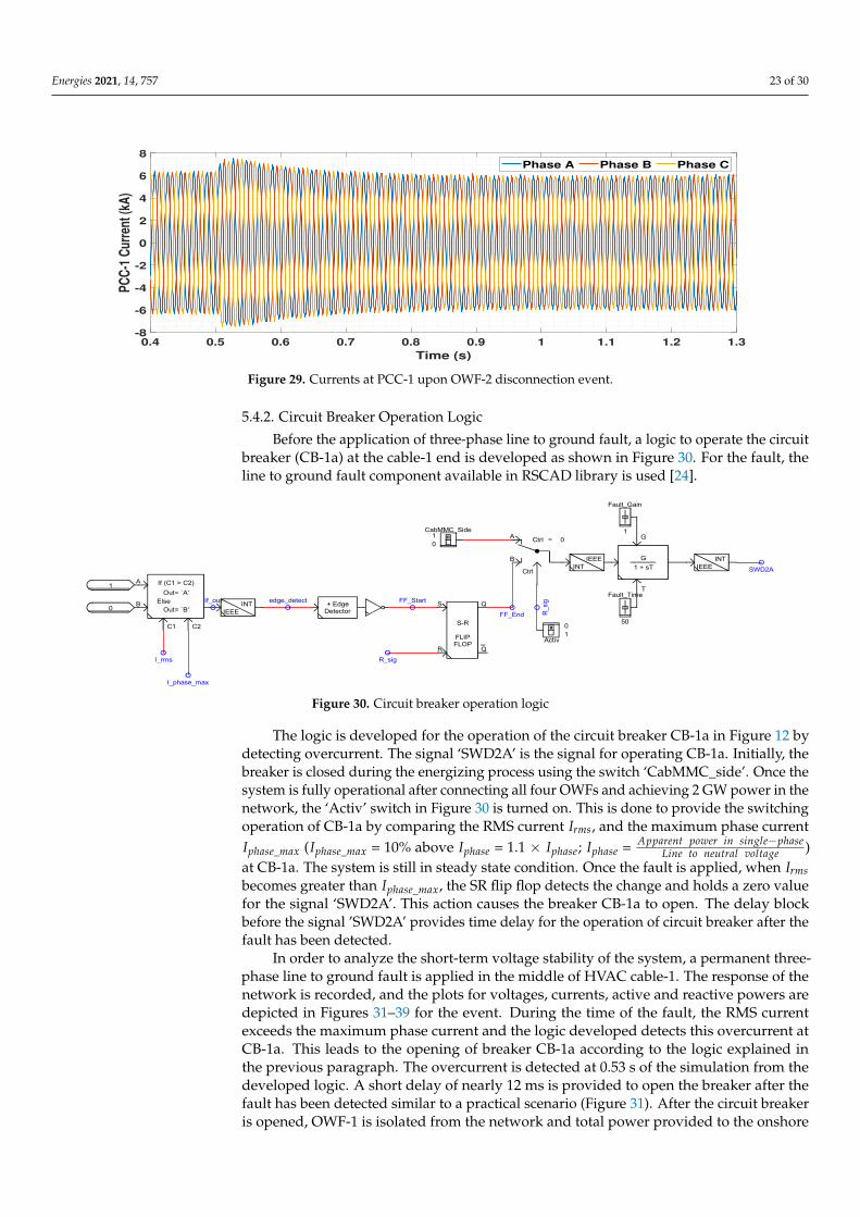
5.4.2. Circuit Breaker Operation Logic

Before the application of three-phase line to ground fault, a logic to operate the circuitbreaker (CB-1a) at the cable-1 end is developed as shown in Figure 30. For the fault, theline to ground fault component available in RSCAD library is used [24].

S-R

FLIPFLOP

S

R

Q

Q

FF_Start

R_sig

+ EdgeDetectorIEEE

INT

A

B

C1 C2

If (C1 > C2)

ElseOut= `A'

Out= `B'

If_out edge_detect

I_rms

I_phase_max

1

0FF_End

CabMMC_Side10

A

B

Ctrl

Ctrl = 0

R_s

ig

INTIEEE

1

Fault_Gain

50

Fault_Time

IEEEINTG

1 + sT

T

G

SWD2A

Activ10

Figure 30. Circuit breaker operation logic

The logic is developed for the operation of the circuit breaker CB-1a in Figure 12 bydetecting overcurrent. The signal ‘SWD2A’ is the signal for operating CB-1a. Initially, thebreaker is closed during the energizing process using the switch ‘CabMMC_side’. Once thesystem is fully operational after connecting all four OWFs and achieving 2 GW power in thenetwork, the ‘Activ’ switch in Figure 30 is turned on. This is done to provide the switchingoperation of CB-1a by comparing the RMS current Irms, and the maximum phase currentIphase_max (Iphase_max = 10% above Iphase = 1.1 × Iphase; Iphase = Apparent power in single−phase

Line to neutral voltage )at CB-1a. The system is still in steady state condition. Once the fault is applied, when Irmsbecomes greater than Iphase_max, the SR flip flop detects the change and holds a zero valuefor the signal ‘SWD2A’. This action causes the breaker CB-1a to open. The delay blockbefore the signal ’SWD2A’ provides time delay for the operation of circuit breaker after thefault has been detected.

In order to analyze the short-term voltage stability of the system, a permanent three-phase line to ground fault is applied in the middle of HVAC cable-1. The response of thenetwork is recorded, and the plots for voltages, currents, active and reactive powers aredepicted in Figures 31–39 for the event. During the time of the fault, the RMS currentexceeds the maximum phase current and the logic developed detects this overcurrent atCB-1a. This leads to the opening of breaker CB-1a according to the logic explained inthe previous paragraph. The overcurrent is detected at 0.53 s of the simulation from thedeveloped logic. A short delay of nearly 12 ms is provided to open the breaker after thefault has been detected similar to a practical scenario (Figure 31). After the circuit breakeris opened, OWF-1 is isolated from the network and total power provided to the onshore

Energies 2021, 14, 757 24 of 30

system is reduced. The total power in the pre-fault period is nearly 2 GW, and after thefault, the total power is reduced to nearly 1500 MW. Similarly to the disconnection of oneOWF, discussed earlier in Section 5.4.1, the power flow is reduced through MMC-1 asshown by the blue line in Figure 32. It is worth of mentioning that the network is stable byviewing the stable voltage in the post-fault period in MMC bus, as shown in Figure 33.

0.4 0.5 0.6 0.7 0.8 0.9 1 1.1 1.2 1.3

Time (s)

-40

-30

-20

-10

0

10

20

30

40

CB

-1a

Cu

rre

nt

(kA

)

Phase A

Phase B

Phase C

0.48 0.5 0.52 0.54 0.56 0.58 0.6

-30

-20

-10

0

10

20

30

40

0.53 s

Figure 31. Currents in circuit breaker (CB-1a) upon three-phase line to ground fault in the middle of cable-1.

0 0.5 1 1.5 2 2.5 3 3.5 4 4.5 5

Time (s)

-200

0

200

400

600

800

1000

1200

1400

Ac

tiv

e p

ow

er

(MW

)

MMC-1

MMC-2

Figure 32. Active power in MMC-1 bus and MMC-2 bus upon three-phase line to ground fault in the middle of cable-1.

0.4 0.5 0.6 0.7 0.8 0.9 1 1.1 1.2 1.3

Time (s)

-80

-60

-40

-20

0

20

40

60

80

MM

C B

us

Vo

lta

ge

(k

V)

Phase A Phase B Phase C

Figure 33. Voltages at MMC bus upon three-phase line to ground fault in the middle of cable-1.

Energies 2021, 14, 757 25 of 30

0.4 0.5 0.6 0.7 0.8 0.9 1 1.1 1.2 1.3

Time (s)

-20

-15

-10

-5

0

5

10

15

20

MM

C-1

Cu

rre

nt

(kA

)

Phase A Phase B Phase C

(a) Currents in MMC-1 bus

0.4 0.5 0.6 0.7 0.8 0.9 1 1.1 1.2 1.3

Time (s)

-30

-20

-10

0

10

20

30

MM

C-2

Cu

rre

nt

(kA

)

Phase A Phase B Phase C

(b) Currents in MMC-2 bus

Figure 34. Currents in (a) MMC-1 bus and (b) MMC-2 bus upon three-phase line to ground fault in the middle of cable-1.

0 0.5 1 1.5 2 2.5 3 3.5 4 4.5 5

Time (s)

0

0.2

0.4

0.6

0.8

1

1.2

PC

C-1

Vo

lta

ge

(p

u)

Voltage

Figure 35. Voltage in p.u. at PCC-1 upon three-phase line to ground fault in the middle of cable-1.

Energies 2021, 14, 757 26 of 30

0.4 0.5 0.6 0.7 0.8 0.9 1 1.1 1.2 1.3

Time (s)

-10

-5

0

5

10

PC

C-1

Cu

rre

nt

(kA

)

Phase A Phase B Phase C

Figure 36. Currents in PCC-1 upon three-phase line to ground fault in the middle of cable-1.

0 0.5 1 1.5 2 2.5 3 3.5 4 4.5 5

Time (s)

0

0.2

0.4

0.6

0.8

1

1.2

1.4

1.6

PC

C-2

Vo

lta

ge

(p

u)

Voltage

Figure 37. Voltage in p.u. at PCC-2 upon three-phase line to ground fault in the middle of cable-1.

0.4 0.5 0.6 0.7 0.8 0.9 1 1.1 1.2 1.3

Time (s)

-10

-5

0

5

10

PC

C-2

Cu

rre

nt

(kA

)

Phase A Phase B Phase C

Figure 38. Currents in PCC-2 upon three-phase line to ground fault in the middle of cable-1.

Energies 2021, 14, 757 27 of 30

0 0.5 1 1.5 2 2.5 3 3.5 4 4.5 5

Time (s)

-2

-1.5

-1

-0.5

0

0.5

1

1.5

2

PC

C-1

Cu

rre

nt

(pu

)

Id

Iq

Figure 39. Currents in d and q axes in PCC-1 upon three-phase line to ground fault in the middle of cable-1.

Increase in active power in MMC-2 after the fault has been cleared, can be explainedby viewing the current profiles in the OWFs detailed in the following paragraph. A majorobservation can be derived from the profile of transients during the fault in the currents ofboth the MMCs in Figure 34a,b. The initial rise in current till 0.53 s is due to the occurrenceof the three-phase fault. The breaker is opened at 0.542 s. The profile of currents at nearly0.59 s are complementary in both MMCs, i.e., the currents are decreasing in MMC-1 andincreasing in MMC-2. This is due to the difference in control strategies in MMC-1 (V/Fcontrol) and MMC-2 (active power control).

Analyzing at the OWFs side of the network, the DVC is modelled to provide ratedreactive current to flow to the fault location by controlling the voltage of the GSC. From thevoltage in p.u. in Figure 35, it can be seen that the voltage at the PCC-1 drops and remainslow throughout the fault period. During the time of fault in cable-1 and after CB-1a isopened, the voltage angle and magnitude at PCC-1 goes to zero. The PLL in GSC-1 issynchronized with the AC voltage at PCC-1. The voltage magnitude at GSC-1 remainsnon-zero, and the voltage angle is zero during the time of fault as the PLL follows theangular reference at PCC-1. Therefore, due to higher voltage magnitude at GSC-1 thanat PCC-1, reactive power will flow from GSC-1 to PCC-1, and since the voltage angle iszero at GSC-1 and PCC-1, active power transmitted is zero during the time of the fault.This is performed in DVC by controlling the d-axis reference voltage of GSC-1 and therebyindirectly controlling the current coming out of the GSC-1 to PCC-1. The current limitationalgorithm implemented in the DVC limits the output current to the rating of the converterand hence rated reactive current flows from the GSC-1 as seen in Figure 36.

Voltages at PCC-2, 3 and 4 have transients during the time of fault and are thenstabilized to a slightly higher value than the pre-fault state to compensate for the lossof OWF-1. This is due to the fast local voltage control in DVC as seen for the case ofdisconnection of one OWF. The post-fault voltage value is within the tolerance limit(±10%), and it can be viewed from the graphs in Figure 37. An important observation inthe voltage graphs of OWFs-2, 3 and 4 is the occurrence of spikes right after the circuitbreaker CB-1a is opened, as can be seen in Figure 37. There can be two reasons for such aphenomenon to occur. The first is that after the circuit breaker CB-1a is opened, reactivecurrent injection still takes place (at 0.59 s in Figure 38 for PCC-2) and this causes thevoltage at the corresponding PCC also to rise. Such a rise in voltage is not applicable inreal-world OWFs and is, therefore, a drawback due to the OWF modelling. These spikescan be ignored as they do not represent the performance of the real hardware. The secondreason could be due to two control strategies that provide the voltage reference in thenetwork. It is seen that during the steady state and post-fault condition, the V/F controlis dominant and provides the voltage reference in the network. However, during thetime of the fault, DVC in all OWFs takes the role of providing the voltage reference in the

Energies 2021, 14, 757 28 of 30

corresponding PCCs, as seen in PCC-1 during the time of three-phase line to ground faultin cable-1. The sudden change back to the steady state condition after the fault is releasedcould lead to discrepancies between the V/F mode and the DVC. The conflict betweenthese control strategies occur as to which control strategy provides the voltage referenceright after the circuit breaker is open and hence this causes a spike in voltage at the PCCs.

The currents from the OWFs-2, 3 and 4 are the same in the post-fault region as thepre-fault condition (Figure 38 for PCC-2) since the scaling factor for each OWF is still thesame. DVC control in these OWFs operate during the time of fault and limit the currentsby controlling the voltages at corresponding PCCs. Due to the increase in voltage in thepost-fault period at the PCCs-2, 3 and 4, the active power generated also will be higherfrom the OWFs-2, 3 and 4. It is reflected in the increase in active power in MMC-2 as shownin Figure 32. Another important observation is in the profile of transients in currents inPCCs-2, 3 and 4 following the occurrence of the fault. As shown in Figure 38 for PCC-2,the current is limited from 0.5 to 0.54 s during the time of fault. After the breaker hasbeen operated at 0.542 s, the profile of currents (from 0.55 s to 0.6 s) is similar to that ofthe MMC-2 (Figure 34b). This is due to the re-synchronization to the grid by the PLL inMMC-2 control and the PLL in DVC of WG-2, 3 and 4.

In practice, if a three-phase fault occurs in a subsea cable, it is hardly that the faultclears on its own and it would require human interference. During such critical islandingsituations, the DVC allows rated reactive current to flow to the fault location by controllingthe GSC voltage and thereby protecting the converters in the OWF from high overcurrents.Based on the reference grid codes mentioned in [8], during steady state operation, theactive current must be the priority, and during the time of the fault, the priority mustbe changed to reactive current. The major takeaway is that the DVC follows the reactivecurrent injection requirement during the time of the fault, as shown from the currents inPCC-1 in Figure 39, even while working in coordination with other control strategies in thenetwork. Current is limited to the rated current of the converter by the current limitationalgorithm in DVC without the requirement of any external controls.

6. Conclusions

In this paper, the development of a large scale EMT model of a 2 GW offshore networkin RSCAD is explained in detail. The modifications in the control structures of the MMCsto work in coordination with the implemented DVC in WGs are addressed. The operationof the developed large scale 2 GW network is discussed. The interplay of offshore MMCsand Type-4 WGs in terms of dynamic power flow control within the offshore network (byanalyzing the voltage and current profiles in the electrical path between the WGs and theMMCs) is performed. The coordination between the V/F control in MMC-1, active powercontrol in MMC-2 and the DVC in OWFs provide a synchronized operation during thesteady state and dynamic conditions in the network. One of the highly severe conditions isthe disconnection of one OWF. In that situation, it is observed that the network remainsstable following the disconnection and the power flowing through MMC-1 reduces as it isworking in V/F control, i.e., capable of providing and absorbing power. Another highlysevere event is the three-phase line to ground fault in one of the HVAC cables. A circuitbreaker logic is modelled to isolate OWF-1 from the network when the fault occurs inHVAC cable-1. It is observed that the operation of the entire network remains stable duringthe pre-fault condition where active current is injected, or can be termed as active powergenerated by all the OWFs. During the time of fault in HVAC cable-1, circuit breaker at theend of the cable is opened upon detection of overcurrent and thereby, islanding OWF-1.The fast local voltage control in DVC in OWF-1 provides voltage support during the timeof the fault, and due to the grid conditions, the reactive current is injected by OWF-1 tothe fault location. The currents are limited to the current rating of the GSC to avoid thedamage of the components in the converter. Hence, it can be concluded that the V/Fcontrol provides the voltage reference during the pre-fault and post fault condition for thenetwork and DVC provides voltage reference at the corresponding PCC when the OWF

Energies 2021, 14, 757 29 of 30

is islanded. Such a generic model provides scope for expansion to a larger scale of 4 GW.The practicality of the DVC can be tested by performing Hardware In Loop testing of theimplemented DVC in a properly set-up test bench. The model also allows to incorporateother control strategies, and studies related to the interoperability of these controllers,coordination with MMC control strategies and higher order contingencies (for e.g., shortcircuit of two or more WGs, disconnection of two or more WGs) can be performed asfuture work.

Author Contributions: Conceptualization, S.G., A.P. and J.R.T.; formal analysis, S.G., A.P. and J.R.T.;investigation, S.G., A.P. and J.R.T.; methodology, S.G., A.P. and J.R.T.; resources, S.G., A.P. andJ.R.T.; software, S.G., A.P. and J.R.T.; supervision, J.R.T., A.P., A.L., P.P. and M.v.d.M.; validation,S.G., A.P. and J.R.T.; visualization, S.G., A.P. and J.R.T.; writing—original draft, S.G., A.P. and J.R.T.;writing—review & editing, S.G., A.P., A.L., J.R.T., P.P and M.v.d.M. All authors have read and agreedto the published version of the manuscript.

Funding: This research received no external funding.

Data Availability Statement: Data sharing not applicable.

Acknowledgments: This research was fully funded by Delft University of Technology. The authorsthank the experts and technical support staff of RTDS Technologies Inc. and DIgSILENT GmbH forthe insightful discussions during the execution of this research.

Conflicts of Interest: The authors declare no conflict of interest. The funders had no role in the designof the study; in the collection, analyses, or interpretation of data; in the writing of the manuscript, orin the decision to publish the results.

References1. UNFCCC. Adoption of the Paris agreement. COP. In 25th Session Paris; UNFCCC: Rio de Janeiro, Brazil; New York, NY, USA,

2015; Volume 30. Available online: https://unfccc.int/sites/default/files/english_paris_agreement.pdf (accessed on 29 January2021).

2. Vision—North Sea Wind Power Hub. 2020. Available online: https://northseawindpowerhub.eu/vision/ (accessed on 26January 2021).

3. TenneT Develops First 2 GW Offshore Grid Connection with Suppliers. Daily Offshore Wind News, 13 February 2020.4. The First Hub-and-Spoke Energy Island—North Sea Wind Power Hub. 2020. Available online: https://northseawindpowerhub.

eu/the-first-hub-and-spoke-energy-island/ (accessed on 26 January 2021).5. Bolik, S.; Ebner, G.; Elahi, H.; Gomis Bellmunt, O.; Hjerrild, J.; Horne, J.; Kilter, J.; Rimez, J.; Temtem, S.; Visiers Guixot, M. HVDC

Connection of Offshore Wind Power Plants; Technical Brochure 619; CIGRE Working Group B4.55. 2015. Available online:https://e-cigre.org/publication/619-hvdc-connection-of-offshore-wind-power-plants (accessed on 29 January 2021).

6. Peralta, J.; Saad, H.; Dennetière, S.; Mahseredjian, J.; Nguefeu, S. Detailed and Averaged Models for a 401-level MMC-HVDCsystem. IEEE Trans. Power Deliv. 2012, 27, 1501–1508. [CrossRef]

7. Telaretti, E.; Graditi, G.; Ippolito, M.; Zizzo, G. Economic feasibility of stationary electrochemical storages for electric billmanagement applications: The Italian scenario. Energy Policy 2016, 94, 126–137. [CrossRef]

8. Mohseni, M.; Islam, S.M. Review of international grid codes for wind power integration: Diversity, technology and a case forglobal standard. Renew. Sustain. Energy Rev. 2012, 16, 3876–3890. [CrossRef]

9. HVDC Technology for Offshore Wind is Maturing; ABB: Zürich, Switzerland, 2018. Available online: https://new.abb.com/news/detail/8270/hvdc-technology-for-offshore-wind-is-maturing (accessed on 26 January 2021).

10. Korai, A.W. Dynamic Performance of Electrical Power Systems with High Penetration of Power Electronic Converters: Analysisand New Control Methods for Mitigation of Instability Threats and Restoration. Ph.D. Thesis, Universität Duisburg-Essen,Duisburg, Germany, 2019. [CrossRef]

11. Lescale, V.; Holmberg, P.; Ottersten, R.; Hafner, Y. Parallelling offshore wind farms HVDC ties on offshore side. Proc. CIGRE 2012 2012.12. Ganesh, S.; Perilla, A.; Torres, J.; Palensky, P.; van der Meijden, M. Validation of EMT Digital Twin Models for Dynamic Voltage

Performance Assessment of 66 kV Offshore Transmission Network. Appl. Sci. 2021, 11, 244. [CrossRef]13. RTDS Technologies Inc. Novacor. 2020. Available online: https://knowledge.rtds.com/hc/en-us/articles/360034290474

-NovaCor- (accessed on 26 January 2021).14. Vrana, T.K.; Yang, Y.; Jovcic, D.; Dennetière, S.; Jardini, J.; Saad, H. The CIGRE B4 DC grid test system. Electra 2013, 270, 10–19.15. World’s Most Powerful Offshore Wind Turbine: Haliade-X 12 MW | GE Renewable Energy. 2020. Available online: https:

//www.ge.com/renewableenergy/wind-energy/offshore-wind/haliade-x-offshore-turbine (accessed on 26 January 2021).16. RTDS Technologies Inc. PB5 Card. 2020. Available online: https://knowledge.rtds.com/hc/en-us/articles/360034285894-PB5

-Card (accessed on 26 January 2021).

Energies 2021, 14, 757 30 of 30

17. Ryndzionek, R.; Sienkiewicz, L. Evolution of the HVDC Link Connecting Offshore Wind Farms to Onshore Power Systems.Energies 2020, 13, 1914. [CrossRef]

18. CIGRE Working Group B4.37. VSC Transmission. Technical Brochure 269. 2005. Available online: https://e-cigre.org/publication/269-vsc-transmission (accessed on 26 January 2021).

19. RTDS Technologies Inc. MMC Modeling. 2020.Available online: https://knowledge.rtds.com/hc/en-us/articles/360039628773-MMC-Modeling (accessed on 26 January 2021).

20. Sharifabadi, K.; Harnefors, L.; Nee, H.P.; Norrga, S.; Teodorescu, R. Design, Control, and Application of Modular Multilevel Convertersfor HVDC Transmission Systems; John Wiley & Sons: Hoboken, NJ, USA, 2016.

21. Erlich, I.; Korai, A.; Neumann, T.; Koochack Zadeh, M.; Vogt, S.; Buchhagen, C.; Rauscher, C.; Menze, A.; Jung, J. New Control ofWind Turbines Ensuring Stable and Secure Operation Following Islanding of Wind Farms. IEEE Trans. Energy Convers. 2017,32, 1263–1271. [CrossRef]

22. CIGRE Working Group B4.57. Guide for the Development of Models for HVDC Converters in a HVDC Grid. Tech. Rep. 2014.Available online: https://e-cigre.org/publication/604-guide-for-the-development-of-models-for-hvdc-converters-in-a-hvdc-grid (accessed on 26 January 2021).

23. Saad, H.A. ModÉlisation et Simulation D’Une Liaison Hvdc de Type Vsc-Mmc. Ph.D. Thesis, Polytechnique Montréal, Montreal,QC, Canada, 2015.

24. RTDS Technologies Inc. RSCAD Modules. 2020. Available online: https://knowledge.rtds.com/hc/en-us/articles/360037537653-RSCAD-Modules (accessed on 26 January 2021).