generating high frequency trading strategies with arti cial …mas02mb/cognitive...
TRANSCRIPT

Generating high frequency trading strategies
with arti�cial neural networks and testing them
through simulation
September 24, 2010
A comparison of second order training methods for time series modelling
Nicolas Dickreuter - University of London, Goldsmiths College
MSc in Cognitive Computing and Arti�cial Intelligence
Abstract
Various backpropagation algorithms are used to test whether a weak
or a semi-strong form of the e�cient market hypothesis can be rejected in
trying to predict stock market returns with neural networks. First training
algorithms such as Levengerg-Marquardt, Bayesian Regularization, BFGS
Quasi-Newton and various (scaled) conjugate gradient gradient methods
are used to train a network. In a second step the result is simulated to
see whether the neural network can outperform a simple buy-and-hold
strategy. Three examples are presented. In the �rst two, past returns of
the Dow Jones Industrial average are used to predict future returns; in the
�rst case with a 3-day and in the second case with a 1-day time horizon.
In the third example input neurons are fed �nancial data of individual
stocks, such as p/e, p/b and dividend payout ratios. The neural network
then optimizes how a constant amount of money is allocated between
stocks of the S&P100. While the di�erent training methods converge to
an optimum at di�erent speeds and to di�erent degrees, some of them
can be described as being more e�cient than others. However, in all the
examples and all the methods, a simple, passive buy-and-hold strategy
1

has not been outperformed by a neural network over the entire period.
Much more imporant than the backpropagation training method of the
neural network is the actual model speci�cation. The aim of this thesis is
much more to lay the grounds of a theoretical framework how potential
strategies need to be tested before they can be con�rmed to be working,
rather than �nding actual working strategies.
2

Contents
1 Introduction 6
2 Theoretical Framework 8
2.1 E�cient market hypothesis (EMH) - expectations based on
other research . . . . . . . . . . . . . . . . . . . . . . . . . . 8
2.2 Development of trading strategies . . . . . . . . . . . . . . . 10
2.3 Out of sample testing . . . . . . . . . . . . . . . . . . . . . 11
2.4 Procedure of the simulation . . . . . . . . . . . . . . . . . . 12
2.4.1 Simulation with di�erent parameters after training
of the network . . . . . . . . . . . . . . . . . . . . . 12
2.4.2 Calculation of returns . . . . . . . . . . . . . . . . . 13
2.4.3 Calculation of other metrics . . . . . . . . . . . . . . 14
2.4.4 Necessity of statistical testing . . . . . . . . . . . . . 14
2.4.5 Non parametric test . . . . . . . . . . . . . . . . . . 15
3 Neural networks 16
3.1 Structure and properties of neural networks . . . . . . . . . 16
3.1.1 Neural networks vs. other statistical methods . . . . 16
3.1.2 Structure . . . . . . . . . . . . . . . . . . . . . . . . 17
3.1.3 Activation function . . . . . . . . . . . . . . . . . . . 18
3.1.4 Momentum . . . . . . . . . . . . . . . . . . . . . . . 18
3.1.5 Learning Rate . . . . . . . . . . . . . . . . . . . . . 19
3.1.6 Threshold function . . . . . . . . . . . . . . . . . . . 19
3.2 Handling of time series . . . . . . . . . . . . . . . . . . . . . 19
3.3 Preprocessing of data . . . . . . . . . . . . . . . . . . . . . . 20
3.3.1 Normalization . . . . . . . . . . . . . . . . . . . . . . 20
3.3.2 Absolute vs. relative changes . . . . . . . . . . . . . 20
3.3.3 Generalization . . . . . . . . . . . . . . . . . . . . . 21
3.3.4 Division of data . . . . . . . . . . . . . . . . . . . . . 22
3.4 Postprocessing and assessment . . . . . . . . . . . . . . . . 22
3.4.1 Performance function - mean square error . . . . . . 22
4 Training algorithms 23
4.1 Overview . . . . . . . . . . . . . . . . . . . . . . . . . . . . 23
4.1.1 Presented methods . . . . . . . . . . . . . . . . . . . 23
4.1.2 Application in Matlab . . . . . . . . . . . . . . . . . 24
4.2 Gradient Descent . . . . . . . . . . . . . . . . . . . . . . . . 25
4.3 Gradient Descent with Momentum . . . . . . . . . . . . . . 27
4.4 Variable Learning Rate Gradient Descent . . . . . . . . . . 27
3

4.5 Gauss Newton method . . . . . . . . . . . . . . . . . . . . . 28
4.6 Levenberg-Marquardt . . . . . . . . . . . . . . . . . . . . . 29
4.7 Bayesian Regularization . . . . . . . . . . . . . . . . . . . . 30
4.8 BFGS Quasi-Newton . . . . . . . . . . . . . . . . . . . . . 31
4.9 Resilient Backpropagation (Rprop) . . . . . . . . . . . . . . 32
4.10 One Step Secant . . . . . . . . . . . . . . . . . . . . . . . . 33
4.11 Conjugate Gradient Algorithms . . . . . . . . . . . . . . . . 34
4.11.1 General notes . . . . . . . . . . . . . . . . . . . . . . 34
4.11.2 Scaled Conjugate Gradient . . . . . . . . . . . . . . 35
4.11.3 Conjugate Gradient with Powell/Beale Restarts . . . 35
4.11.4 Fletcher-Powell Conjugate Gradient . . . . . . . . . 36
4.11.5 Polak-Ribiére Conjugate Gradient . . . . . . . . . . 36
5 Implemented Matlab Classes 36
5.1 Neural network . . . . . . . . . . . . . . . . . . . . . . . . . 36
5.2 Simulator . . . . . . . . . . . . . . . . . . . . . . . . . . . . 37
6 Empirical results of neural network strategies 39
6.1 Overview . . . . . . . . . . . . . . . . . . . . . . . . . . . . 39
6.2 Expected sum of returns of the next 3 days . . . . . . . . . 39
6.2.1 Setup . . . . . . . . . . . . . . . . . . . . . . . . . . 39
6.2.2 Results . . . . . . . . . . . . . . . . . . . . . . . . . 40
6.2.3 Statistical signi�cance of out of sample test . . . . . 41
6.3 10 past days as input predicting next day . . . . . . . . . . 41
6.3.1 Setup . . . . . . . . . . . . . . . . . . . . . . . . . . 41
6.3.2 Results . . . . . . . . . . . . . . . . . . . . . . . . . 42
6.4 High frequency trading example: multiple �nancial factors
as input neurons . . . . . . . . . . . . . . . . . . . . . . . . 42
6.4.1 Setup . . . . . . . . . . . . . . . . . . . . . . . . . . 42
6.4.2 Results . . . . . . . . . . . . . . . . . . . . . . . . . 43
6.4.3 Statistical signi�cance of out of sample test . . . . . 43
7 Conclusion 44
7.1 Summary of results . . . . . . . . . . . . . . . . . . . . . . . 44
7.2 Suggested future research . . . . . . . . . . . . . . . . . . . 44
A Figures for strategy 1: 3-day forecast based on past prices 46
B Figures for Strategy 2: 1 day price forecast based on past
prices 55
C Figures for Strategy 3: forecast based on �nancial factors 63
4
D Program Listings 70
D.1 Neural Network . . . . . . . . . . . . . . . . . . . . . . . . . 70
D.1.1 Neural Network Main program (training) [training.m] 70
D.1.2 Neuron Class [Neuron.m] . . . . . . . . . . . . . . . 72
D.1.3 Neuron Class [NeuronNewton.m] . . . . . . . . . . . 76
D.1.4 Forward Propagation Function [NeuronCalc.m] . . . 77
D.1.5 Sigmoid function [sigmoid.m] . . . . . . . . . . . . . 78
D.1.6 Neural Network Training with Toolbox [train_matlab1.m] 78
D.1.7 Neural Network Training with Toolbox [train_matlab3.m] 80
D.2 Trading Simulator . . . . . . . . . . . . . . . . . . . . . . . 82
D.2.1 Main program [main.m] . . . . . . . . . . . . . . . . 82
D.2.2 TimeSeries Class [Time_series.m] . . . . . . . . . . 85
D.2.3 Trade Generator Class [TradeGenerator.m] . . . . . 88
D.2.4 Trade Analyzer Class [TradeAnalyzer.m] . . . . . . . 91
D.2.5 Trade Graph generator Class [TradeGraphs.m] . . . 96
D.2.6 Trade Class [Trade.m] . . . . . . . . . . . . . . . . . 103
D.2.7 Fund Class [FundReturn.m] . . . . . . . . . . . . . . 104
D.2.8 Strategy Class [STRATEGY_NeuralNetwork1.m] . 108
D.2.9 Strategy Class [STRATEGY_NeuralNetwork2.m] . 109
D.2.10 Strategy Class [STRATEGY_NeuralNetwork3.m] . 111
E Figures, Tables and Bibliography 114
5

1 Introduction
When forecasting the future of markets we can broadly distinguish between two
categories: a) strategies which rely on historical data such as prices, volume of
trading or volatility and b) fundamental analysis, which is based on external in-
formation from the economic system, such as company �nancial, interest rates,
pro�tability ratios of the companies and other micro- and macroeconomic data.
The use of technical analysis is mostly frowned upon in academic circles. The
e�cient markets hypothesis (EMH) asserts that the price of an asset re�ects
all of the information that can be obtained from past prices of the asset. Any
opportunity for a pro�t will be exploited immediately and hence disappear. De-
spite the controversial reputation of technical analysis, it still �nds respectable
application among amateur traders, and professionals in the equity world often
base their trading decisions on historical prices, among other information (oth-
erwise, why would anybody look at price charts?). If there are some patterns
which lead indeed to an outperformance, they should be detectable with the
help of neural networks. It is the goal of this thesis to describe how such a
trading strategy would have to be developed and tested for validity.
The �rst part (Chapter 2) describes the theoretical �nancial framework
which is used as a basis to forecast prices with the help of neural networks.
In Chapter 3 general properties of neural networks are described and in Chap-
ter 4 the di�erent training algorithms which are used in the analysis are de-
scribed, and how generally neural networks and the simulator are programmed
on Chapter 5.
I then show empirical results in Chapter 6 how the neural networks can be
used to test the strong form of the e�cient market hypothesis in trying to make
predictions of the Dow Jones Industrial when only taking price as an input
and empirically test the application of neural networks to trading strategies.
Two such examples are presented. In a third example the input neurons are no
longer past prices, but rather �nancial factors of individual stocks. The neural
network should then decide how a �xed amount of money should be allocated
among stocks of the S&P100.
First a network is trained to recognize buying and selling signals. This is
done with a variety of di�erent training algorithms that are described in more
detail. The trained neural network is then implemented into a simulator which
calculates trading results with various parameters in the threshold function,
which activates buying and selling signals. The calculated optimal parameters
6

which are extracted through numerical approximation are then used as a trading
strategy. In order to claim that a trading strategy is potentially working in a
real-life environment, it needs to be tested for statistical signi�cance in an out-
of-sample test.
Finally the conclusion (Chapter 7) ends the thesis with a summary of the
�ndings.
7
2 Theoretical Framework
2.1 E�cient market hypothesis (EMH) - expectations based
on other research
The E�cient market hypothesis assumes that �nancial markets are information-
ally e�cient and that excess market return cannot be generated consistently
through any strategy.
There are three forms of the EMH: The weak, the semi-strong and the strong
form. In the weak form, future prices can't be predicted simply by analyzing
past prices and no excess returns can be achieved in the long run using historical
price data only. In other words technical analysis won't be able to produce
abnormal returns when the weak form of the EMH is assumed to be holding
but other forms such as insider trading and fundamental analysis may still be
applied successfully.
The semi-strong form of the EMH implies that all publicly available informa-
tion, meaning not just historical prices but also company or securities speci�c
information is included in the current price, making it impossible to outperform
the market not just by technical analysis, but also by fundamental analysis.
Whenever a new piece of information about a security or any of its underlyings
becomes available, this would be incorporated into the price instantly.
To test for strong-form e�ciency, a market needs to exist where investors
cannot consistently earn excess returns over a long period of time. Even if some
money managers are consistently observed to beat the market, no refutation
even of strong-form e�ciency follows: with hundreds of thousands of fund man-
agers worldwide, even a normal distribution of returns (as e�ciency predicts)
should be expected to produce a few dozen "star" performers.
Various research papers have disputed the e�cient-market hypothesis, both
on empirical and theoretical basis. For example �Behavioral economists� claim
that factors such as overcon�dence, overreaction, representative bias, informa-
tion bias, and various other predictable human errors can cause distortions
which could potentially be exploited from investors recognizing them. Empiri-
cal evidence has been mixed, but has generally not supported strong forms of
the e�cient-market hypothesis. (Nicholson [Jan/Feb 1968], Basu [1977], Rosen-
berg B [1985], Fama E [1992], Michaely R [1993])
Other papers have shown that P/E ratios can have in�uence on stock re-
turns N. and A. [1992] and other company speci�c (or �fundamental� factors)
8

have been identi�ed to have potentially predictive power on stock returns. While
only a fraction of academic research in the �eld has been able to produce abnor-
mal return in empirical application, any such market ine�ciency would auto-
matically vanish once the volume of the pro�t generating trades is high enough.
That's why it is very likely that if any neural network could �nd a successful
strategy from the past, it may potentially only last for a short period of time
because market participants quickly exploit it.
In this thesis I aim to show how a weak and semi-strong form of the EMH
could be rejected or accepted with the help of neural networks. In the �rst case
I only use past prices of the Dow Jones Industrial as input neurons. If the neural
network would �nd any strategy which could outperform the market, the weak
form of the EMH would be rejected. Given the large amount of research which
does have con�rmed the weak form of EMH, this would be unexpected when
based purely on plain vanilla equity instruments.
When taking fundamental factors (company speci�c �nancial information)
into account the neural networks are set up to reject or accept the semi-strong
EMH. As in this analysis only a fraction of the available information about
the companies' �nancials are used in the model, it won't be possible to draw
any de�nitive conclusions from the results. Moreover, the forthcoming analy-
ses should give a framework under which potential market ine�ciencies can be
tested for possible exploitation. Research in this domain is mixed and opinions
are polarized very strongly. Advocates of an ine�cient market often point to
start fund managers and skeptics often try to highlight the fact that ex-post
academic analyses are often �awed and biased. When looking at the perfor-
mance of professionally managed funds, where many of them take fundamental
factors into consideration, it is in my view very unlikely that a semi-strong form
of the EMH can be rejected. The reason behind this is based on two factors:
1. Market complexity is generally underestimated. To be able to predict the
outcome of a stock price based on a small number of factors is intuitively
impossible when assuming the following: When hitting a billiard ball on a
table and trying to predict the second or third bounce is relatively simple in
reality and can be replicated in a laboratory. However, the ninth bounce,
an equation that includes every single person around is needed, because
the gravitational pull of a man will impact the trajectory. The equation
will get signi�cantly more complex. To predict the 53rd bounce of the
billiard ball on the table every single elementary particle in the universe
9

needs to be part of the equation. There is no question that to predict
the future price of a stock is more complicated that predicting the 53rd
bounce of a billiard ball (Taleb [2007]).
2. Large, unpredictable (exceptional) events (black swans) have a signi�cant
in�uence on returns. �Based on data for the Dow Jones Industrial Average
over the last 107 years, is unequivocal: outliers have a massive impact on
long-term performance. Missing the best 10 days resulted in portfolios
65% less valuable than a passive investment, whereas avoiding the worst
10 days resulted in portfolios 206% more valuable than a passive invest-
ment.�Estrada [2009]. It appears that the outliers are the decisive events
rather than the small �uctuations. Those outliers are per de�nition un-
expected and would not be predicted by any related variables, even when
statistical signi�cance is given. That's why any investment approach based
on a neural network (or probably worse: based on normal distribution and
linear regression) would most likely fail in the long run.
Nevertheless, it is possible that a neural network may spot some market ine�-
ciencies that could reject the weak form of the EMH for a short period of time.
It would be virtually impossible to transform this into a pro�t in a real-world
environment, but I'd like to outline the theoretical framework that could be
applied to identify such ine�ciencies and then test them on statistical signi�-
cance. While passing the tests would still be no guarantee of potential success
in a real environment, failing them would have to lead to an exclusion of the
active strategy.
2.2 Development of trading strategies
In order to test whether the neural network can generate a trading strategy, we
need to give some framework under which the strategy is developed. Since the
neural network can only act within its own model speci�cations, it helps when
some economic intuition is behind the data that is fed to the input neurons.
As outlined above, historical prices are only one factor that is potentially of
value. Intuitively (although not necessarily so in reality) additional factors
should improve the performance of the neural network.
In this paper the following strategies are being testes:
1. Buying and selling signal given through a 3-day forward looking neural
network, taking into consideration the returns that will be earned over
10

the next 3 days as output neuron, and the last 5 days as input neurons.
This strategy is based on the Dow Jones Industrial Index.
2. Buying and selling signal given through a 1-day forward looking neural
network, considering the next day's return as output neuron and the last 10
days as input neurons. This strategy is based on the Dow Jones Industrial
Index.
3. Buying and selling signal given through a network which takes 3 �nancial
factors of di�erent companies into consideration. The output neuron is
connected to the next day's return of the respective stocks. This strategy
is based on individual stocks of the S&P100.
2.3 Out of sample testing
Once the network has been trained with a subset of the dataset, the neural
network needs to be tested with an out-of-sample application. It is generally
agreed that for forecasting methods out-of sample tests rather than goodness of
�t to past data (in-sample tests) should be used. The performance of a model on
data outside of that used in its construction and training remains the ultimate
touchstone which determines its validity. There are two arguments as shown
by[Tashman, 2001]:
For a given forecasting model, in-sample errors are likely to understate fore-
casting errors. Estimation and method selection are designed to calibrate a
forecasting procedure. This leads to the problem that in many cases the small
nuances of past history are not repeated in the future and other occurrences
which may occur in the future may not be part of the training sample. Needless
to say, this can have a strong impact on the performance of the model.
In addition common extrapolative forecasting methods, such as exponential
smoothing or also neural networks, are based on updating procedures, in which
one makes each forecast as if one were standing in the immediately prior period.
For updating methods, the traditional measurement of goodness-of-�t is based
on one step-ahead errors - errors made in estimating the next time period from
the current time period. Real time assessment has practical limitations for fore-
casting practitioners, since a long wait may be necessary before a reliable picture
of a forecasting track record will materialize. As a result, tests based on holdout
samples have become commonplace. If the forecaster withholds all data about
events occurring after the end of the �t period, the forecast-accuracy evaluation
11

is structurally identical to the real-world-forecasting environment, in which we
stand in the present and forecast the future. However, taking already into con-
sideration the held-out data while selecting the forecasting method pollutes the
evaluation environment.
2.4 Procedure of the simulation
2.4.1 Simulation with di�erent parameters after training of the net-
work
Once the neural network has been trained, its e�ectiveness needs to be tested
with a trading simulation. It is not enough to just look at the mean square
error of the trained neural network but an actual simulation is imperative. In
our case the testing is done with a custom built simulator in Matlab where
di�erent strategies can be easily de�ned in rewriting the respective class.
While the total trading performance is the most important factor to look at,
it is crucial to see it in the context with what the strategy actually does, such
as the amount of total trades, % of winning trades and % of days long. As a
benchmark we always take a simple buy-and-hold strategy (passive investment
strategy) which can always be achieved at much lower cost as there is only
minimal infrastructure necessary. In the active strategy the model assumes a
2% risk free rate, meaning that when the index (or security) is sold, a 2% p.a.
return can be achieved.
12

Figure 2.1: Procedure of simulation
There are 3 steps in the actual simulation:
1. The simulation takes the trained neural network and varies the di�erent
threshold parameters for the buying and selling decision individually (see
Fig. 3.3 on page 19 for examples of threshold functions).
2. An optimal strategy will evolve. In Fig 2.1 we can see at the bottom left
how the total annual return of the strategy will peek for some parame-
ters. This strategy will need to be further investigated as it is the most
promising one.
3. The optimal strategy is tested for statistical signi�cant outperformance
versus a buy-and-hold strategy in an out of sample test.
2.4.2 Calculation of returns
There are two ways to calculate the return between t and t+1. For the purposes
to calculate cumulative abnormal return, the compounded return (i.e. logarith-
mic) presents the distinctive advantage that di�erent time periods of return can
be added up in order to calculate the return of a cumulative period. Unless
stated otherwise I use for all calculations in this paper compounded returns:
13

R := LN
(StSt+x
)= LN(St)− LN(Xt+x)
St is the stock price (or index price) at day t. With the given calculation each
strategy is compared with a buy-and-hold approach of the same securities and
a number of di�erent metrics are calculated as outlined below. Returns are
calculated in the TimeSeries class right after the excel �les are loaded.
2.4.3 Calculation of other metrics
� The total performance of a given trading strategy is calculated in summing
up the individual logarithmic returns of the generated trades, such as
Rs = (∑ni=1Ri)+R
fx where Ri depicts the return of each individual trades
from 1 . . . n and Rfxthe risk free return of the period where no trade was
open.
� The total strategy performance p.a. is the annualized version of the above:
Rsp = Rs
totaldays · 365
� The total risk free return Rf for period xis calculated as Rfx = Rf · xwhere x constitutes the amount of idle days where no trade is open.
� The number of idle days is calculated as TSn −∑T di where TSnis the
total amount of returns of the time series and T di the duration of trade i.
� The buy-and-hold performance is simply calculated in summing up all the
individual returns of the time series or Rb =Log(TSstop)Log(TSstart)
� The buy-and-hold performance p.a. is calculated as Rbp = Rb
totaldays · 365
� The out-performance p.a. Rop is calculated as Rop = Rsp −Rpb
The calculations above are taking place in the Trade Analyzer class and is listed
in Chapter D.2.4 on page 91.
2.4.4 Necessity of statistical testing
In order to determine whether the neural network's generated trading perfor-
mance is better than a random strategy, we need to test the result for statistical
signi�cance.
Hypothesis testing is de�ned by the following general procedure:
14

1. State the relevant null hypothesis. In our case this is µr = µnwhere as
µris the result of a random investment strategy and the µnthe average
return of the strategy developed by the neural network.
2. Statistical assumptions need to be tested. For our purposes what matters
is whether returns are normally distributed. �The normal distribution is
a poor �t to the daily percentage returns of the S&P 500. The log-normal
distribution is a poor �t to single period continuously compounded returns
for the S&P 500, which means that future prices are not log-normally
distributed. However, sums of continuously compounded returns are much
more normal in their distribution, as would be expected based on the
central limit theorem. The t-distribution with location/scale parameters
is shown to be an excellent �t to the daily percentage returns of the S&P
500 Index.� Egan [2007]
3. Decision of which statistical test is applied: Due to the inconclusive results
I use a non-parametric test which is much more lax in terms of statistical
assumptions: The Wilcoxon signed-rank test can be used as alternative to
t-tests when the sample cannot be assumed to be normally distributed.
4. Next the values need to be computed.
5. Decision whether the null hypothesis can be rejected and the returns are
statistically signi�cantly di�erent to 0. Alternatively the null hypothe-
sis cannot be rejected and the Neural network does not outperform the
random strategy
2.4.5 Non parametric test
The Wilcoxon signed-rank test is a statistical hypothesis test for the case of two
related samples or repeated measurements on a single sample. It can be used
as an alternative to the paired Student's t-test when the population cannot be
assumed to be normally distributed. Similar to the paired or related sample
t-test, the Wilcoxon test involves comparisons of di�erences between measure-
ments. The advantage is that it doesn't require assumptions about the form of
the distribution.
The Wilcoxon test transforming each instance of XA −XB into its absolute
value, and removes all the positive and negative signs. In most applications of
the Wilcoxon procedure, the cases in which there is zero di�erence between XA
15

and XB are at this point eliminated from consideration, since they provide no
useful information, and the remaining absolute di�erences are then ranked from
lowest to highest, with tied ranks included where appropriate.
Suppose we collect 2n observations, two observations of each of the n sub-
jects. Let i denote the particular subject that is being referred to and the �rst
observation measured on subject i be denoted by xi and second observation be
yi. For each i in the observations, xi and yi should be paired together. The
null hypothesis tested is H0 : θ = 0. The Wilcoxon signed rank statistic W+ is
computed by ordering the absolute values |Z1| . . . , |Zn| the rank of each ordered
Zi is given a rank of Ri. Denote the positive Zi values with ϕi = I(Zi > 0)
where I(.) is an indicator function. The Wilcoxon signed ranked statistic W+
is de�ned as
W+ =
n∑i=1
φiRi
Tied scores are assigned a mean rank. The sums for the ranks of scores
with positive and negative deviations from the central point are then calculated
separately. A value S is de�ned as the smaller of these two rank sums. S is
then compared to a table of all possible distributions of ranks to calculate p,
the statistical probability of attainingS from a population of scores that is sym-
metrically distributed around the central point. The test statistic is analyzed
using a table of critical values. If the test statistic is less than or equal to the
critical value based on the number of observations n, then the null hypothesis
is rejected in favor of the alternative hypothesis. Otherwise, the null cannot be
rejected. Lowry [2010],Wikipedia [2010]
3 Neural networks
3.1 Structure and properties of neural networks
3.1.1 Neural networks vs. other statistical methods
Neural networks have a similar approach to other statistical methods used for
data modeling1. In all cases it is the goal to limit the number of assumptions
and to use the method to optimize a procedure to �nd the best parameters
to reproduce the results. As described in Carverhill and Cheuk [2003] already
countless research has been made in the �nancial industry where neural networks
1See Riplay [1996] for a general discussion of Neural Networks and its relation to non-parametric estimation methods
16
have been used to forecast option prices (as substitute method for Black-scholes)
or Kwon et al. [2010] used a neural network in an attempt to forecast stock prices.
While it may be possible that neural networks can indeed predict prices more
accurately than other models, research which is actually testing the success of
the neural network in a statistically rigorous manner is very rare.
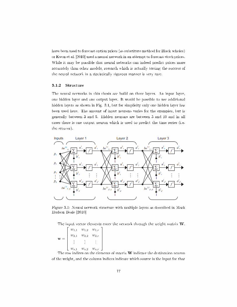
3.1.2 Structure
The neural networks in this thesis are build on three layers. An input layer,
one hidden layer and one output layer. It would be possible to use additional
hidden layers as shown in Fig. 3.1, but for simplicity only one hidden layer has
been used here. The amount of input neurons varies for the examples, but is
generally between 3 and 5. Hidden neurons are between 5 and 10 and in all
cases there is one output neuron which is used to predict the time series (i.e.
the returns).
Figure 3.1: Neural network structure with multiple layers as described in MarkHudson Beale [2010]
The input vector elements enter the network through the weight matrix W.
w =
w1,1 w1,2 w1,r
w2,1 w2,2 w2,r
......
...
ws,1 ws,2 ws,r
The row indices on the elements of matrixW indicate the destination neuron
of the weight, and the column indices indicate which source is the input for that
17

weight. Before training of the network can start the weights will need to be
initialized with random values.
3.1.3 Activation function
Hidden layers are using the sigmoid activation function which is de�ned as
P (x) = 11+e−xHaykin [2009]. Experiments have also been made with the TanH
function, but no signi�cant di�erence could be found in the results. The com-
parison of the two functions is shown in Fig. 3.2. The output neuron is using
a linear activation function which is sometimes activating the signal through a
threshold as is further explained in Chapter 3.1.6.
-10 -8 -6 -4 -2 0 2 4 6 8 100
0.1
0.2
0.3
0.4
0.5
0.6
0.7
0.8
0.9
1
(a) Sigmoid function
-10 -8 -6 -4 -2 0 2 4 6 8 10-1
-0.8
-0.6
-0.4
-0.2
0
0.2
0.4
0.6
0.8
1
(b) TANH function
Figure 3.2: Activation functions
3.1.4 Momentum
Momentum is used to stabilize the weight change by making nonradical revi-
sions using a combination of the gradient decreasing term with a fraction of
the previous weight change: This gives the system a certain amount of inertia
since the weight vector will tend to continue moving in the same direction un-
less opposed by the gradient term. The momentum smooths the weight changes
and suppresses cross-stitching, that is cancels side-to-side-oscillations across the
error valley. When all weight changes are all in the same direction the momen-
tum ampli�es the learning rate causing a faster convergence. Momentum also
enables to escape from small local minima on the error surface. We can de�ne
momentum as follows:
wij = w′ij + (1−M) · LR · ej ·Xj +M · (w′ij − w′′ij)
18

The results of the neural network (in this case the gradient descent back-
propagation method) has not been strongly in�uenced on whether momentum
has been applied or not. This is mainly a dependent on the form of the error
surface as described above. An example of where momentum would have an
e�ect is shown in the error surface of Fig. 4.2 on page 27.
3.1.5 Learning Rate
In the program a learning rate of η = 0.1 has been found to be a good measure
to start. Depending on the backpropagation method the learning rate performs
di�erent functions. The variable learning rate method experiments with a non-
constant learning rate.
3.1.6 Threshold function
θ denotes the threshold. In the simulation the optimal threhold is found out
through experimentation. When the output neuron passes a threshold, a buying
or selling action is performed.
(a) Binary activation function
0 50 100 150 200 250 300 3500
0.2
0.4
0.6
0.8
1
1.2
1.4
(b) Example of binary activation function
Figure 3.3: Threshold functions
3.2 Handling of time series
In order for the program to be able to handle the time series, a variety of addi-
tional enhancements need to be implemented: In the gradient descent method
each datasets leads to an adjustment of the weights. The time series then moves
one step forward and the input neurons are adjusted accordingly. Input neu-
19
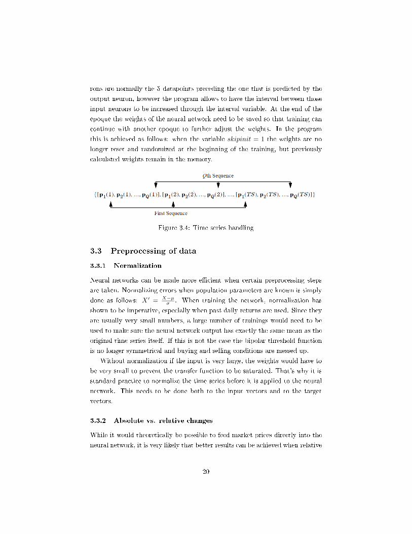
rons are normally the 5 datapoints preceding the one that is predicted by the
output neuron, however the program allows to have the interval between those
input neurons to be increased through the interval variable. At the end of the
epoque the weights of the neural network need to be saved so that training can
continue with another epoque to further adjust the weights. In the program
this is achieved as follows: when the variable skipinit = 1 the weights are no
longer reset and randomized at the beginning of the training, but previously
calculated weights remain in the memory.
Figure 3.4: Time series handling
3.3 Preprocessing of data
3.3.1 Normalization
Neural networks can be made more e�cient when certain preprocessing steps
are taken. Normalizing errors when population parameters are known is simply
done as follows: X ′ = X−µσ . When training the network, normalization has
shown to be imperative, especially when past daily returns are used. Since they
are usually very small numbers, a large number of trainings would need to be
used to make sure the neural network output has exactly the same mean as the
original time series itself. If this is not the case the bipolar threshold function
is no longer symmetrical and buying and selling conditions are messed up.
Without normalization if the input is very large, the weights would have to
be very small to prevent the transfer function to be saturated. That's why it is
standard practice to normalize the time series before it is applied to the neural
network. This needs to be done both to the input vectors and to the target
vectors.
3.3.2 Absolute vs. relative changes
While it would theoretically be possible to feed market prices directly into the
neural network, it is very likely that better results can be achieved when relative
20

changes to previous periods (i.e. log returns as described in 2.4.2 on page 13) are
used, especially as the returns are more likely to approach a normal distribution
than the prices themselves.
0 0.5 1 1.5 2 2.5 3
x 104
101
102
103
104
105
(a) Dow Jones Industrial Average 1929-2008:Absolute values in log scale
0 0.5 1 1.5 2 2.5 3
x 104
-0.3
-0.25
-0.2
-0.15
-0.1
-0.05
0
0.05
0.1
0.15
(b) Dow Jones Industrial Average 1929-2008:daily log returns
Figure 3.5: Absolute values vs. relative returns
For the purpose of exploiting the strong form of the EMH (for further details
see Chapter 2.1 on page 8) it makes sense to use a normalized form of logarithmic
returns as we want to extract buying and selling signals. For that we need to
know what happens to the returns R in the period t + x. An example of the
results from a trained network see A.14 on page 52.
3.3.3 Generalization
A well trained network should be able to give good answers even with inputs
that have not been seen during the training. The more similar the new input is
to the ones that have been used during training, the better are the answers. To
improve generalization there are two features that can be used:
1. Early stopping: It is important that the network is not overtrained, as
this will lead to much worse results when being applied with untrained
input data. In Matlab early stopping can be automatically handled in
monitoring the error of the validation set while training on the train-
ing set. Training is then stopped when the validation increases over
net.trainParam.max_fail iterations (maximum number of validation In-
creases).
21

2. Regularization: Regularization can be done by using the Bayesian regular-
ization training function. Any data in the valuation set should be moved
to the training set.
3.3.4 Division of data
When training multilayer networks, the general practice is to �rst divide the
data into three subsets. The �rst subset is the training set, which is used for
computing the gradient and updating the network weights and biases. The
second subset is the validation set where the error on the validation set is mon-
itored during the training process. The validation error should decrease during
the initial phase of training, as does the training set error. However, when the
network begins to over�t the data, the error on the validation set begins to
rise. The test set error (which constitutes the third type of dataset) is not used
during training. If the error on the test set reaches a minimum at a signi�cantly
di�erent iteration number than the validation set error, this might indicate a
poor division of the data set. The division can be done in blocks, randomly,
using interleaved sections or by data index. (Mark Hudson Beale [2010])
3.4 Postprocessing and assessment
3.4.1 Performance function - mean square error
A good initial assessment for the neural network is the mean square error (MSE)
which gives us indication how the di�erent training epoques improved its per-
formance. It is de�ned as follows:
MSE =1
N
n∑i=1
(ti − ai)2
While it is generally desirable to reduce the MSE as much as possible, over-
�tting may quickly become a problem when the network is trained too much.
An enhancement to the above function gives us the the Bayesian Regularization
approach involves modifying the usually used objective function. As shown in
Chi Dung Doan [2009] the modi�cation can enhance the model's generalization
capability in expanding the term. Ew which is the sum of the square of the
network weights.
Matlab o�ers a variety of tools to further test the validity of the network. The
foundations for this are already laid in the steps where the data is preprocessed
22

and the data is split into training, validation and testing set for each epoch for
each of the training sets and continues progress of the neural network should
be observable. Ideally the validation and test MSE should develop in a similar
manner. If the test curve had increased signi�cantly before the validation curve
increased, then it would be an indication that over�tting had occurred. An
example is shown in Fig. A.5 on page 48 where a repetitive pattern is used as
input to BFGS quasi newton method. In Fig. A.14 on page 52 we can see the
di�erence of the results when various training methods are used.
4 Training algorithms
4.1 Overview
4.1.1 Presented methods
While some of the training algorithms were programmed from scratch, I have
taken the liberty to use some of the integrated Matlab functions, as they o�er
much greater e�ciency and speed and also �exibility. The following methods
have been used for testing:
Function Algorithm
trainlm Levenberg-Marquardttrainbr Bayesian Regularizationtrainbfg BFGS Quasi-Newtontrainrp Resilient Backpropagationtrainscg Scaled Conjugate Gradienttraincgb Conjugate Gradient with Powell/Beale Restartstraincgf Fletcher-Powell Conjugate Gradienttraincgp Polak-Ribiére Conjugate Gradienttrainoss One Step Secanttraingdx Variable Learning Rate Gradient Descenttraingdm Gradient Descent with Momentumtraingd Gradient Descent
Table 1: Training algorithms used for testing
Each of the training algorithms have their advantages and disadvantages.
While for the overall performance of the trading simulator the actual training
algorithm may only have an insigni�cant e�ect, as other factors, such as quality
of data and correctness of the model speci�cation (i. e. picking the relevant
23

data) is much more important. Nevertheless, for completeness's sake I analyze
the performance of the di�erent algorithms and give a short assessment on what
their e�ects are when used with returns on the Dow Jones Industrial Average.
It is complex and and time consuming to compute the Hessian matrix for
feedforward neural networks. Algorithms that are based on Newton's method,
do not require calculation of second derivatives. These are called quasi-Newton
(or secant) methods. They update an approximate Hessian matrix at each
iteration of the algorithm. The update is computed as a function of the gradient.
The quasi-Newton method that has been most successful in published studies is
the Broyden, Fletcher, Goldfarb, and Shanno (BFGS) update. This algorithm
is implemented in the trainbfg routine.Mark Hudson Beale [2010]
The training algorithms all aim to reduce the error produced by the neural
network in �nding a way to strive to the ideally global minimum of the n-
dimensional error surface.
Figure 4.1: Gradients of a vector �eld
4.1.2 Application in Matlab
At �rst network and weights need to be initialized and then the network can
be trained. The network can be trained for function approximation (nonlinear
regression), pattern association, or pattern classi�cation. A set of examples with
network input p and target t is required.
For batch gradient descent the traingd function is used. The weights will be
updated in the direction of the negative gradient.
There are seven training parameters associated with traingd :
� epochs: number of epochs
� show: The training status is displayed for every show iterations of the
24

algorithm
� goal: The training stops if the number of iterations exceeds epochs, if the
performance function drops below goal
� time: Training stops after a certain amount of time
� min_grad: Training stops if gradient falls below min_grad
� max_fail: If training is lager than maxfail
� lr: The learning rate lr is multiplied times the negative of the gradient to
determine the changes to the weights
The network is trained on the training data until its performance begins to
decrease on the validation data, which signals that generalization has peaked.
The test data provides a completely independent test of network generalization
(Mark Hudson Beale [2010]).
4.2 Gradient Descent
Weights and biases are updated in the direction of the negative gradient of the
performance function which is the direction where the performance function
decreases the most.
Gradient descent iteratively updates w replacing wt by wt+1 using the fol-
lowing update equation where η is a learning rate that typically declines with
t. wt+1 = wt − η∇L. Note that here we are minimizing L so we want to move
in the opposite direction from the gradient.
wt+1 = wt − ηtw∂L∂wj
(Mark Hudson Beale [2010] use the notation as follows: xk+1 = xk − αkgk
where xk is a vector of the current weights and gk is the current gradient and
αk is the learning rate.)
Through one-dimensional optimization wj is adjusted while holding the other
weights �xed. We do this for each j and because the weights have changed, we
may need to repeat the process until all weights are simultaneously at optimal
values.
For a normal multilayer perceptron with incremental method the following
method has been applied in the computer program:
25

1. A training sample if presented to the neural network which is normalized.
X ′i =[xiµi
σi
]2. The z-score normalization uses the mean and the standard deviation for
each feature across a set of training data.This produces data where each
feature has a zero mean and a unit variance.Priddy [2005]. For our given
purposes this appears to be the method of normalization which makes the
most sense.
3. The desired output is compared to the actual output after forward prop-
agation.
4. β is calculated for each node The beta for the TanH equals β = q ·y ·(1−y),where q is the weighted sum of the betas of the following layer, where the
respective network is connected to. The weights are given by the weights
of the connection themselves. y denotes the output signal.
5. The weights of each connection are adjusted with the delta, which is cal-
culated as follows: 4 = βi · η · yxy(in the program listing this is neu-
ron(id).beta * learningRate * neuron(neuron(id).connections(n)).outputsignal)
6. The previous steps are repeated until the mean square error is no longer
decreasing. This prevents over�tting.
Minimization by gradient descent is based on the linear approximation E(w +
y) ≈ E(w) + E′(w)T y, which is the main reason why the algorithm is often
inferior to other methods. In addition the algorithm uses constant step size,
which in many cases are ine�cient.
A simple form of gradient descent su�ers from serious convergence problems.
Ideally we should be able to take steps as large as possible down to the gradient
where it is small (small slope) and and take smaller steps when the gradient
is large, so that we don't jump of of the minimum. With the update rule of
the gradient descent we do right the opposite of that. In addition to that the
curvature of the error surface may not be the same in all directions. A long and
narrow valley for example the motion could be more along the wall (bouncing
from one wall to the other) even though we want to move as fast as possible
out of the valley without bouncing the walls. This can be improved with not
only using gradient information but also the curvature (i.e. second derivatives).
(Ranganathan [2004])
26

(a) Error function with local minima as de-scribed in Rojas [1996]
(b) Gradient descent method(green) vs. conjugate gradientillustration (red) as shown inAlexandrov [2010]
Figure 4.2: Moving on the error surface: method comparison
4.3 Gradient Descent with Momentum
In adding momentum to the gradient descent method, the network can also
respond to recent trends in the error surface. In that sense momentum can
ignore small features on the error surface and act like a lowpass �lter. It will
help to avoid that the network gets stuck in a shallow local minimum that could
be slid through with momentum. (Mark Hudson Beale [2010]).
Including a momentum term in the algorithm is a way to force the algo-
rithm to use second order information from the network. Unfortunately the
momentum term is not able to speed up the algorithm considerable, and may
cause the algorithm to be even less robust, because of the inclusion of another
user dependent parameter, the momentum constant (Møller [1990]). This is in
accordance with the observations made in this paper as is visible in Fig. A.12
compared to Fig.A.13.
4.4 Variable Learning Rate Gradient Descent
This method uses a variable learning rate η that is adjusted depending on how
the performance of the network evolves during training. η is decreased whenever
27

performance has increased while if performance deteriorates η is increased. As
calculation normal gradient descent backpropagation is used as described in
Chapter 4.2 is used.
4.5 Gauss Newton method
The Gauss�Newton algorithm is a method used to solve non-linear least squares
problems. It can be seen as a modi�cation of Newton's method for �nding a
minimum of a function. Unlike Newton's method, the Gauss�Newton algorithm
can only be used to minimize a sum of squared function values, but it has
the advantage that second derivatives, which can be challenging to compute,
are not required. The Gauss�Newton algorithm will be derived from Newton's
method for function optimization via an approximation. As a consequence,
the rate of convergence of the Gauss�Newton algorithm is at most quadratic.
The recurrence relation for Newton's method for minimizing a function S of
parameters, β is βs+1 = βs − H−1g where g denotes the gradient vector of
S and H the hessian matrix of S. Elements of the Hessian are calculated by
di�erentiating the gradient gj = 2∑mi=1
(ri
ariaβi
)with respect to Bk Hjk =
2∑mi=1
(ariaβj
ariaβk
+ ria2ri
aβiaβk
).
In order to apply the hessian matrix to the neural network the following
methodology has been applied in the computer program
1. Through normal forward propagation the values of each nodes are calcu-
lated.
2. βj is calculated for each node. For the output nodes βj always takes the
value 1. For the inner nodes it will take the value of βj = qi ·(1−y2) whereqi is again the weighted sum of the following betas (assuming there might
be more than one output node) weighted by the connection's weight.
3. Two vectors are calculated for each dataset whereas each value depicts
one weight of the network Jn = βjn · yn and Gnβn · yn. J in this case is
recalculated for each dataset, while G is cumulatively added and averaged
at the end of the dataset.
4. The Hessian Matrix is calculated for each dataset so that H = J ′ · J and
is summed up with each dataset (as in Matlab the vector is a column, the
multiplication needs to be J ′ · J and not vice versa).
28

5. The hessian matrix is summed up and averaged at the end of the batch.
To avoid a singular matrix a small value is added to the diagonal of the
Hessian after which the deltas can be calculated.
6. At the end of each epoque the delta is calculated in multiplying the G with
the inverse hessian. (In Matlab this can be accelerated with d = g/H)
4.6 Levenberg-Marquardt
As described in Mark Hudson Beale [2010], similar to the quasi-Newton method,
the Levenberg-Marquardt algorithm is designed to approach second-order train-
ing speed without having to compute the Hessian matrix. Levenberg-Marquardt
can be thought of as a combination of steepest descent and the Gauss-Newton
method. When the current solution is far from the correct one, the algorithm be-
haves like a gradient descent method: slow, but guaranteed to converge. When
the current solution is close to the correct solution, it becomes a Gauss-Newton
method.
The Hessian matrix is approximated as H = JTJ and the gradient g = JTe
where J is the Jacobian matrix that contains �rst derivatives of the network
errors with respect to the weights and biases and e is a vector of network errors.
In vector calculus, the Jacobian marix is the matrix of all �rst-order partial
derivatives of a vector- or scalar-valued function with respect to another vector.
In our case it contains the �rst derivatives of the network errors with respect to
the weights and biases.
J(n) =
∂e(1)∂w1
∂e(1)∂w2
∂e(1)∂w3
· · · ∂e(1)∂wm
∂e(2)∂w1
∂e(2)∂w2
∂e(2)∂w3
· · · ∂e(2)∂wm
∂e(3)∂w1
∂e(3)∂w1
∂e(3)∂w1
· · · ∂e(3)∂wm
......
.... . .
...∂e(n)∂w1
∂e(n)∂w2
∂e(n)∂w3
· · · ∂e(n)∂wm
w=w(n)
The importance of the Jacobian lies in the fact that it represents the best
linear approximation to a di�erentiable function near a given point. It is the
derivative of a multivariate function. For a function of n variables, n > 1, the
derivative of a numerical function must be matrix-valued, or a partial deriva-
tive.Haykin [2009]
29

Finally, the weights are updated as follows:
xk+1 = xk −[JTJ+ µI
]−1JTe
.
With a µ is zero the method coincides with Newton's method using the
Hessian Matrix as approximation as shown in Chapter 4.5 and implemented
manually in Matlab as shown in Chapter D.1.3. With a large µ the method
become identical to gradient descent with a very small step size. In di�erent
positions on the error surface, one or the other method is at an advantage.
Generally it is Newton's method that is faster and more accurate near an error
minimum, which means a shifting towards that method is desired as quickly as
possible. That's why µ is increased after each successful step.
4.7 Bayesian Regularization
Bayesian regularized neural networks have the advantage that they are di�cult
to overtrain, as an evidence procedure provides an objective criterion for stop-
ping training. They are di�cult are inherently insensitive to the architecture
of the network, as long as a minimal architecture has been provided. It has
also been shown mathematically that they do not need a test set, as they can
produce the best possible model most consistent with the data (Burden and
Winkler [2009]).
In our case the network training function updates the weight and bias values
according to Levenberg-Marquardt optimization. Backpropagation is used to
calculate the Jacobian jX of performance perf with respect to the weight and bias
variables X. Each variable is adjusted according to Levenberg-Marquardt,Mark
Hudson Beale [2010].
jj = jX * jX
je = jX * E
dX = -(jj+I*mu) \ je
where E is all errors and I is the identity matrix. The adaptive value mu is
increased by mu_inc until the change shown above results in a reduced perfor-
mance value.
In bayesian regularization training not only aims to minimize the sum of
squared errors but instead adds an additional term. The objective function
30

becomes
F = βEd + αEw
where Ewis the sum of squares of the network weights and Edis the sum
of the squared errors. αand β are coe�cients giving di�erent weights to the
optimization functions. There is a trade o� between reducing the errors more
emphasizing network size reduction, which will produce a smoother network
response. It minimizes a combination of squared errors and weights, and then
determines the correct combination so as to produce a network that generalizes
well.
4.8 BFGS Quasi-Newton
As described in Schoenberg [2001], Sir Isaac Newton applied calculus was the
optimization of a function. in observing that the derivative of a function being
zero gave its extremum. The problem is that �nding this extremum for non-
quadratic functions is not always easy. Newton proposed an iterative solution
in using a Taylor series approximation about some given point of the function's
surface. If the function is quadratic, we arrive at the solution in a single step.
If the function is not quadratic, we must solve it iteratively. While I don't want
to go into further detail how the actual Newton method is working exactly, it is
su�cient to understand that the inverse of the Hessian will determine the angle
of the direction and the gradient. The issue comes from the fact that a function
for computing an analytical Hessian is almost never available and that's why
methods have been developed to compute it numerically.
The BFGS Quasi Newton method is a variation of Newton's optimization
algorithm, in which an approximation of the Hessian matrix is obtained from
gradients computed at each iteration of the algorithm.
As described in Mark Hudson Beale [2010] the BFGS Quasi-Newton method's
backpropagation adjusts the weights and biases as X = X + a · dX where dX
is the search direction. The parameter a is selected to minimize the perfor-
mance along the search direction. A line search function is used to locate the
minimum point while the �rst search direction is the negative of the gradient
of performance. In succeeding iterations the search direction is computed as
dX = −H/(gX)−1 where gX is the gradient and H is a approximate Hessian
31
matrix. The Hessian matrix is de�ned as:
H(f) =
∂2f∂x2
1
∂2f∂x1∂x2
. . . ∂2f∂x1∂xn
∂2f∂x2∂x1
∂2f∂x2
2. . . ∂2f
∂x2∂xn
......
. . ....
∂2f∂xn∂x1
∂2f∂xn∂x2
. . . ∂2f∂x2
n
To compute the Hessian matrix is relatively complex and can take a lot of
resources. Quasi-Newton methods avoid the calculation in updating an approx-
imate Hessian matrix at each iteration. The update is computed as a function
of the gradient. The BFGS is the quasi-Newton method which has been most
successful.
The procedure is described in detail in Edwain K.P. Chong [2008].
Hk = Hk−1 +
(yyT
yT s
)− Hk−1ss
THk−1
sTHk−1s
H−1k =
(I − syT
yT s
)H−1k−1 −
(I − ysT
yT s
)+ssT
yT s
where s = x(k) − x(k−1)
Like other methods, the BFGS method can also get stuck on a saddle-point.
In Newton's method, a saddle-point can be detected during modi�cations of
the (true) Hessian. Therefore, search around the �nal point when using quasi-
Newton methods.
4.9 Resilient Backpropagation (Rprop)
Neural networks usually use sigmoid or TanH transfer functions (activation func-
tions in the hidden layer). As a side e�ect they sometimes compress a large
input range into a limited output range. In both Sigmoid and TanH functions
the slopes approach zero when the input gets large. This causes the gradient to
have a very small magnitude and therefore weights and biases are changed only
slightly from their original value.
The resilient backpropagation tries to mitigate these side e�ects of the partial
derivatives. The principle works as follows: Only the sign of the derivative of
the error function can determine the direction of the weight update while the
magnitude of the derivative has no e�ect on the weight update. The size of the
weight change is determined by a separate update value which is decreased by
32

a constant factor whenever the derivative with respect to that weight changes
sign from the previous iteration. If the derivative is zero, the update value will
remain the same. The e�ect is a decreasing oscillation that updates the weight
as whenever an oscillation occurs, the weights change is reduce. If the weight
continues to change in the same direction for several iterations, the magnitude
of the weight change increases.
Each variable is adjusted according to the following: dX = deltaX ·sign(gX)
where the elements of deltaX are all initialized to delta0, and gX is the gradi-
ent. At each iteration the elements of deltaX are modi�ed.(Mark Hudson Beale
[2010])
As described in Riedmiller [1994], for Faster Backpropagation Learning: The
RPROP Algorithm, each weight has an individual update value 4ij which de-
termines the up.
4w(t)ij =
−4ij, ∂e∂wij
> 0
+4ij , ∂e∂wij
< 0
w(t)ij = w
(t)ij +4w(t)
ij
If the partial derivative changes sign, meaning that the previous step was
too large and the minimum was missed, the previous weight-update is reverted:
4w(t)ij = −4w(t+1)
ij ,∂e
∂wij
(t+1)
· ∂e
∂wij
(t)
< 0
4.10 One Step Secant
The term secant methods used in is reminiscent of the fact that derivatives
are approximated by the secants through two function values although in many
dimensions the function values here the function is the gradient do not determine
uniquely the secant here the approximated Hessian.
Weights and biases are adjusted as follows in the backpropagation as de-
scribed in Mark Hudson Beale [2010]:
X = X+a∗dX where dX is the search direction. The parameter a is selected
to minimize the performance along the search direction. A line search function
is used to locate the minimum point. The �rst search direction is the negative
of the gradient of performance. In succeeding iterations the search direction is
computed from the new gradient and the previous steps and gradients, according
33

to the following formula:
dX = −gX +Ac ∗Xstep+Bc ∗ dgX; where gX is the gradient, Xstep is the
change in the weights on the previous iteration, and dgX is the change in the
gradient from the last iteration.
4.11 Conjugate Gradient Algorithms
4.11.1 General notes
As described in Mark Hudson Beale [2010]the basic backpropagation algorithm
adjusts the weights in the steepest descent direction (negative of the gradient),
the direction in which the performance function is decreasing most rapidly.
While the function decreases most rapidly along the negative of the gradient, it
does not produce the fastest convergence.
In the conjugate gradient algorithms a search is performed along conjugate
directions, which produces generally faster convergence than steepest descent
directions. In most of the algorithms the learning rate η is used to determine
the lenght of the weight update. In conjugate gradient algorithms the step
size is adjusted at each iteration. A line search determines the step size that
minimizes the performance function. Repeated line searches work well when the
following condition is satis�ed: ∂2f∂wj∂wk
= 0. The conjugate gradient method
does line searches along the conjugate directions given by the eigenvectors of
the Hessian.Haykin [2009]
In conjugate gradient methods and quasi-Newton methods the descent path
is not determined by the steepest gradient and a line search routines have to be
applied. The search routines have to be applied several times for each individual
search, which makes the conjugate gradient methods time-consuming. As a
positive factor the methods have a convergence which is usually much quicker
as less iterations are needed. They become particularly interesting for large
scale networks.
A bisection algorithm is the simplest version of a line search but has usually
quite poor performance. The golden section search does not require calculation
of the slope either. It just starts by determining an interval, beginning at a given
point and extending the interval border in increasing steps until the minimum
of the error function is bracketed. The position of the minimum is estimated
by narrowing down the current interval. However, a combination of a golden
section search and a quadratic interpolation between the intervals is much more
e�ective. It will lead to an asymptotic convergence (Sei�ert [2006]).
34

4.11.2 Scaled Conjugate Gradient
As described in Møller [1990], who developed the algorithm, ,the scaled conju-
gate gradient method distinguishes itself form the other methods in the fact that
it chooses the search direction and step size more carefully by using information
from the second order approximation E(w+y) ≈ E(w)+E′(w)T y+ 12yTE′′(w)y,
where E(w) denotes the error function in a given point (w + y) in RN.
The scaled conjugate gradient algorithm is based on conjugate directions,
but this algorithm does not perform a line search at each iteration which can
potentially safe a lot of time. The method may use more iterations than other
conjugate gradient methods, but the amount of computations can be signi�-
cantly reduced as no line search needs to be performed.
As shown in Mark Hudson Beale [2010] most of the optimization methods
used to minimize functions are based on the same strategy. The minimization is
a local iterative process in which an approximation to the function in a neigh-
borhood of the current point in weight space is minimized. The approximation
is often given by a �rst or second order Taylor expansion of the function. The
error function in minimized as follows (Møller [1990]):
1. Choose initial weight vector w1 and set k = 1
2. Determine a search direction pk and a step size αk so that E(wk+αkpk) <
E(wk)
3. Update vector: w+1 = wk + αkpk
4. If E′(wk) 6= 0 then set k = k + 1 and go to 2 else return wk + 1 as the
desired minimum
Through an iterative process the next point is determined. This takes two
steps: In the �rst one the search direction is determined. It is decided in which
direction the the search in the weight-space should be performed to �nd a new
point. In a second step it has to be determined how far in the speci�ed direction
the search needs to go. If the search direction pk is set to the negative gradient
�E′(w) and the step size αk to a constant e, then the algorithm becomes the
gradient descent algorithm as described in 4.2 on page 25.
4.11.3 Conjugate Gradient with Powell/Beale Restarts
This conjugate gradient method uses a line search to determine the minimum
point. The �rst search direction is the negative of the gradient. In succeed-
35

ing iterations the search direction is computed from the new gradient and the
previous search direction according the the following formula:
dX = −gX+ dXold · Z where gX is the gradient. Z can be computed in
di�erent ways. The Powell-Beale variation of conjugate gradient is distinguished
by two features. First, the algorithm uses a test to determine when to reset the
search direction to the negative of the gradient. Second, the search direction
is computed from the negative gradient, the previous search direction, and the
last search direction before the previous reset. (Mark Hudson Beale [2010])
For all conjugate gradient algorithms, the search direction is periodically
reset to the negative of the gradient. In the Powell/Beale restart method the
restart occurs if there is very little orthogonality left between the current gra-
dient and the previous gradient.
| gTk−1 − gk |≥ θ | gk |2
Whenever this condition is met, the search condition is reset to the negative
of the gradient.
4.11.4 Fletcher-Powell Conjugate Gradient
For the Fletcher-Reeves variation of conjugate gradient it is computed accord-
ing to Z=normnew_sqr/norm_sqr; where norm_sqr is the norm square of the
previous gradient and normnew_sqr is the norm square of the current gradient.
4.11.5 Polak-Ribiére Conjugate Gradient
For the Polak-Ribiére variation of conjugate gradient, it is computed according
to Z = ((gX - gX_old)'*gX)/norm_sqr; where norm_sqr is the norm square of
the previous gradient, and gX_old is the gradient on the previous iteration.
5 Implemented Matlab Classes
5.1 Neural network
In the simplest case we use a gradient descent method: One way to program
the backpropagation algorithm with the �exibility of adjusting the size of the
network is in creating a neuron class that handles all the functions itself and
where the initial structure is set up through properties of the class itself. Once
the Neurons have been instantiated, the addConnection method is called which
36

sets the connections between the neurons and assigns them a certain type. All
the di�erent connections have to be de�ned.
Figure 5.1: UML diagram of Neural Network training
The training can then start in looping through a procedure that �rst calls
the forward propagation. The result is then compared to the desired output
and a backpropagation method is called for all the neurons, �rst for the output
layer, then for each of the neurons in the hidden layer. Once all the β and γ are
calculated, the weights need to be updated. This is done through the weight
updating method.
For the approximate Newton method an additional class (NeutonNeuron) is
made available which inherits the Neuron class with all its functions. The full
listing is provided in Chapter D.1 on page 70.
5.2 Simulator
The trading simulator is fully object oriented and �exible to assess any trad-
ing strategy in changing di�erent parameters and making it easy to assess the
outcome through a 3-dimensional graphical depiction. It consists of a variety of
classes which an overview is given in Fig. 5.2.
37

Figure 5.2: UML diagram of trading simulator
The procedure of the simulation is as follows: At �rst a time series is loaded,
this is done in the TimeSeries class as listed in Chapter D.2.2 on page 85.
Depending on whether only one series (in the case of an index) or multiple
series when various stocks are loaded as in the third example that is presented
below. In a next step the trades are generated, based on the strategy that is
applied. This is done through the TradeGenerator class and its subclass, which
is always a prede�ned strategy. In our case, the strategy class is generating an
output value in the neural network which is then used to make a buying and
selling decision. Once all the trades are generated (which each having properties
such as buying price, selling price and return, etc), the trades need to be bundled
and analyzed. This is the purpose of the trade analyzer class: returns of all the
trades are averaged and summed up and a great variety of analysis is done. The
di�erent metrics that are calculated are described in more detail in Chapter 2.4.3
on page 14.
Once all the di�erent metrics are stored, they have to be graphically dis-
played. This is done by the TradeGraphs class (see Chapter D.2.5 on page 96
for a full listing of the class). The di�culty there lies to understandably depict
the 3d Arrays that were generated by the TradeAnalyzer class. This is best
done with 3d mesh diagrams where all the results are displayed as a function
38

of varying parameters (buying and selling thresholds). In the 3d graphs it is
relatively easy to spot the best trading strategy, which can then be analyzed in
more detail.
Finally it is always of interest for any strategy to see the actual performance
in a simulated scenario, so that the day-to-day behaviour of the hypothetical
fund can actually be observed.
6 Empirical results of neural network strategies
6.1 Overview
As outlined earlier it is questionable whether trying to make predictions based
on price only are a meaningful method of forecasting prices. But to outline a
procedure of how such a testing would have to be done I present some examples
that are simply based on past prices. In a �rst step the neural network is trained
according to a certain rule and in a second step the results are simulated and
assessed.
In total there are 3 examples: the �rst two examples are trying to make
predictions based on past prices only. The �rst one focuses on the following 3
days as a whole, assuming that it might be ine�cient to try to predict what hap-
pens the very next day. The second example focuses on the following day only.
Both of them are trading the Dow Jones Industrial index. The third example
goes beyond only looking at past prices of an index and incorporates �nancial
factors from di�erent companies to decide, which stock should be bought and
sold. The neural network then decides how a given amount of money should be
distributed among 100 di�erent stocks, depending on how the �nancial factors,
which are used as input neurons, evolve.
6.2 Expected sum of returns of the next 3 days
6.2.1 Setup
In this setup the input neurons represent the returns of the last 5 days and the
output neuron is the sum of the returns of the next 3 days. In a �rst step we
need to train the neural network with all available backpropagation algorithms,
so we can decide which was is delivering the best results. Once this is done, the
neural network is saved so we can apply it for further testing.
39

Buying and selling signals are triggered with the binary activation function
when the output neuron exceeds the parameter θband θsfor the buying and
selling thresholds. The optimal thresholds are decided through a simulation
and by trial and error. The results of the simulation are presented in Fig. A.15
on page 53.
As described in [Rojas, 1996] it is of advantage to use a bipolar network in-
stead of a binary one: �Many models of neural networks use bipolar, not binary,
vectors. In a bipolar coding the value 0 is substituted by =1. This change does
not a�ect the essential properties of the perceptrons, but changes the symmetry
of the solution regions. It is well known that the algebraic development of some
terms useful for the analysis of neural networks becomes simpler when bipolar
coding is used.�
6.2.2 Results
Sharp Ratio for Dow Jones of the given period 1.1786Sharp Ratio for simulated Fund 1.3515
peakToTroughLogFund -23.7709peakToTroughLogIndex -23.7709
Statistical signi�cance of di�erence p =0.1759Outperformance p.a. 0.2062
Buy and hold performance p.a. 14.2208Strategy performance p.a. 14.4269Buy and hold longdays 3650Strategy Longdays 3611
Table 2: Strategy 1 Summary
The results of the trained networks can be seen in Chapter A.14 on page 52
and the actual results of the simulation are printed in Chapter A.15 on page 53.
While the above results show that the neural network is not outperforming the
market as such, the good news is that the sharp ratio is actually higher. It
seems that the neural network is able to avoid certain periods of high volatility.
40

6.2.3 Statistical signi�cance of out of sample test
Outperformance p.a. -0.6843Buy and hold performance p.a. -1.9609
Strategy performance p.a. -2.6451Buy and hold longdays 3225Strategy Longdays 3208
Table 3: Strategy 1 Summary (out of sample)
The out of sample results are shown in chapter A.16 on page 54.
6.3 10 past days as input predicting next day
6.3.1 Setup
Similar to the above example, we �rst train the network. The di�erence to
the method user in Chapter 6.2 is that we are using di�erent input and output
neurons. As input neurons we go further back: using the returns of the last 10
days as input neurons. As output neuron on the other hand, we only use the
return on of the following day.
Once the neural network has been trained with all the di�erent backprop-
agation methods, we decide which one was most successful. After that we can
apply the neural network in a testing environment and try to �nd out, at which
threshold level buying and selling signals should be triggered. They are trig-
gered with the binary activation function when the output neuron exceeds the
parameter θband θsfor the buying and selling thresholds. The results of the
simulation are presented in Fig. B.14 on page 62.
41

6.3.2 Results
Sharp Ratio for Dow Jones of the given period 1.19Sharp Ratio for simulated Fund 1.22
peakToTroughLogFund -15.2peakToTroughLogIndex -22.7
Statistical signi�cance of di�erence p =0.63Outperformance p.a. 0.71
Buy and hold performance p.a. 14.3Strategy performance p.a. 15.0Buy and hold longdays 3650Strategy Longdays 3388Number of trades 93
Table 4: Strategy 2 Summary
6.4 High frequency trading example: multiple �nancial
factors as input neurons
6.4.1 Setup
This setup distinguishes itself that it is not simply relying on past prices of
the securities but it takes additional company-speci�c information into account.
In this example we no longer examine an index of securities, but we trade
the actually securities themselves. The sample consists of 100 securities of the
S&P100, for a timeframe of 1980 to 2008, subject to data availability (when one
of the factors is not yet available, the period for that stock is ignored). The
neural network determines how a given amount of money (starting with e.g.
$1000) is distributed among the 100 securities. The neural network is trained
in a way that the 3 input neurons will generate one output signal. If the output
signal increases relative to the previous day, then this is considered a buying
signal. If the output signal decreases to the previous day, it is considered a
selling signal.
When the neural network is trained, the output neuron is connected to the
next day's return of the respective security. If it is relatively high, it will end
up training the network to buy at this point and if it is low, the network will
be trained to sell.
The following factors are fed as input neurons into the neural networks:
1. Change in payout ratio over the last day: The payout ratio of a security
depicts the portion of net income of the company that is distributed as
42

a dividend to stockholders. There is no consensus on whether this factor
has in�uence on future stock price development. Nevertheless, traders
sometimes take it into consideration and base their decisions among others
on this indicator.
2. Change in p/e ratio over the last day: The p/e ratio indicates how a
stock is priced relative to it's projected or past earnings. In our case, the
p/e ratio is calculated in dividing the current stock price by last year's
earnings per share.
3. Change in p/b ratio over the last day: Similar to the p/e ratio, the p/b
ratio refers to a stock's price per book value.
4. Output signal: The output signal is trained to the price change to the
next day
The above factors can be replaced with other factors that may be more appro-
priate. To avoid distortions in the neural network it is important that they are
of the same magnitude as the output neuron (i.e. % change towards it's last
value). If absolute values are taken, they would have to be normalized.
The results of this simulation are presented in Fig. C.13 on page 69.
6.4.2 Results
Outperformance median -6.2Buy and hold median. 10.2
Strategy median 4.0Fund Sharpe Ratio 1.66Index Sharpe Ratio 1.59
Table 5: Strategy 3 Summary
The result in this case shows a clear underperformance. When loking at Fig. C.13
on page 69 we can see that for many of the stocks the amount of winning trades
was less than 50%. The given con�guration is not suitable for a neural network
and the strategy clearly does not work.
6.4.3 Statistical signi�cance of out of sample test
No out of sample test has been performed in this case as the results of the
in-sample test are not satisfactory.
43

7 Conclusion
7.1 Summary of results
Similar to Malikel [1973] view of Technical analysis, it is not possible with a
simple neural network to outperform the market when the input neurons are
based on price only. In addition to that the simulations have shown that neural
networks are unable to outperform the market for an extended period of time
when input neurons are connected to p/e, p/b and payout ratios. However in
one case an increase in the sharp ratio has been observed.
The di�erent training algorithms have shown relatively large divergence in
how they manage to reduce the error. Generally, second order training methods
have been most successful while the gradient descent method is clearly not
suitable for these kind of large scale problems.
Nevertheless, it is not the backpropagation algorithm which makes a dif-
ference whether the market can be outperformed or not, it is much more the
speci�cation of the model itself (i.e. the input neurons and the de�nition of
the output neuron) that are important. If the input factors have no signi�cant
connection to the output factors, there is no use in training the network.
7.2 Suggested future research
In this thesis it was tested whether neural networks could outperform the market
over an extended period of time in using past prices and some �nancial ratios.
While there was no restriction on when the trades should be made, the used
dataset was using end of day prices. The trades were thus limited on a maximum
one one trade per day.
In future research it might make sense to loosen this restriction and allow
multiple trades per day. This would require to signi�cantly enhance the dataset:
using order book data instead of only actual last prices and use them as input
neurons might give a better understanding about the current psychology of the
market. Research in this area is relatively limited because datasets are not
readily available in information systems such as Bloomberg or Factset. It is
likely that when using this additional information and testing the success of a
trained neural network based on order book information for a relatively short
period of time, success rates could be higher than what is presented in the
context of this thesis.
In addition it would be interesting to explore di�erent asset classes. The
44

equity market is generally researched relatively well. Neural networks could
�nd better application when used in connection with derivatives or potentially
also forex products, where data is less prone to be contaminated by accounting
standards as it is the case in the equity market. In addition it would be interest-
ing to include a quanti�ed form of general news�ow. This would be especially
interesting in connection with high frequency trading and detailed information
about order books of individual securities. Since this information is not readily
available, market ine�ciencies are much more likely to surface.
45

A Figures for strategy 1: 3-day forecast based on
past prices
0 10 20 30 40 50 60 70 80 90 10010
-6
10-4
10-2
100
102
Best Validation Performance is 0.21314 at epoch 100
Mea
n S
quar
ed E
rror
(m
se)
100 Epochs
Train
Validation
TestBest
Goal
(a) MSE
-3 -2 -1 0 1
-3
-2
-1
0
1
Target
Out
put~
=-0
.028
*Tar
get+
-0.0
056 Training: R=-0.70084
Data
FitY = T
-1 0 1
-1
0
1
Target
Out
put~
=-0
.024
*Tar
get+
-0.0
06 Validation: R=-0.69564
Data
FitY = T
-1 0 1
-1
0
1
TargetOut
put~
=-0
.026
*Tar
get+
-0.0
063 Test: R=-0.73165
Data
FitY = T
-3 -2 -1 0 1
-3
-2
-1
0
1
TargetOut
put~
=-0
.027
*Tar
get+
-0.0
058 All: R=-0.70303
Data
FitY = T
(b) Regression
Figure A.1: Gradient Descent (Trained network for DJ Industrial's returns 1990-2000)
0 5 10 15 20 25 30 35 40 4510
-6
10-4
10-2
100
Best Validation Performance is 0.00025293 at epoch 43
Mea
n S
quar
ed E
rror
(m
se)
49 Epochs
Train
Validation
TestBest
Goal
(a) MSE
-3 -2 -1 0 1
-3
-2
-1
0
1
Target
Out
put~
=1*
Tar
get+
-4.6
e-00
5 Training: R=0.99956
Data
FitY = T
-1 0 1
-1
0
1
Target
Out
put~
=1*
Tar
get+
-0.0
0086
Validation: R=0.99931
Data
FitY = T
-1 0 1
-1
0
1
Target
Out
put~
=1*
Tar
get+
-0.0
0069
Test: R=0.99953
Data
FitY = T
-3 -2 -1 0 1
-3
-2
-1
0
1
Target
Out
put~
=1*
Tar
get+
-0.0
0025
All: R=0.99952
Data
FitY = T
(b) Regression
Figure A.2: Scaled conjugate gradient (Trained network for DJ Industrials re-turns 1990-2000)
46

0 5 10 15 20 25 30 35 40 4510
-6
10-4
10-2
100
Best Validation Performance is 0.00017199 at epoch 40M
ean
Squ
ared
Err
or
(mse
)
46 Epochs
Train
Validation
TestBest
Goal
(a) MSE
-3 -2 -1 0 1-3
-2
-1
0
1
Target
Out
put~
=0.
0056
*Tar
get+
1.1 Training: R=0.043927
Data
FitY = T
-1 0 1
-1
0
1
Target
Out
put~
=1*
Tar
get+
0.00
047
Validation: R=0.99955
Data
FitY = T
-3 -2 -1 0 1
-3
-2
-1
0
1
Target
Out
put~
=0.
99*T
arge
t+0.
0002
5 Test: R=0.99925
Data
FitY = T
-3 -2 -1 0 1
-3
-2
-1
0
1
Target
Out
put~
=0.
31*T
arge
t+0.
8
All: R=0.24017
Data
FitY = T
(b) Regression
Figure A.3: BFGS quasi Newton (Trained network for DJ Industrials returns1990-2000)
0 0.5 1 1.5 2 2.5 3 3.5 4 4.5 510
-6
10-4
10-2
100
Best Validation Performance is 3.3282e-006 at epoch 5
Mea
n S
quar
ed E
rror
(m
se)
5 Epochs
Train
Validation
TestBest
Goal
(a) MSE
-3 -2 -1 0 1
-3
-2
-1
0
1
Target
Out
put~
=1*
Tar
get+
0.00
099
Training: R=1
Data
FitY = T
-1 0 1
-1
0
1
TargetO
utpu
t~=
1*T
arge
t+0.
001
Validation: R=1
Data
FitY = T
-1 0 1
-1
0
1
Target
Out
put~
=1*
Tar
get+
0.00
1
Test: R=1
Data
FitY = T
-3 -2 -1 0 1
-3
-2
-1
0
1
Target
Out
put~
=1*
Tar
get+
0.00
1
All: R=1
Data
FitY = T
(b) Regression
Figure A.4: Levenberg-Marquardt (Trained network for DJ Industrials returns1990-2000)
47

0 5 10 15 20 25 3010
-6
10-4
10-2
100
102
104
Best Validation Performance is 2.799e-005 at epoch 32M
ean
Squ
ared
Err
or
(mse
)
32 Epochs
Train
Validation
TestBest
Goal
(a) MSE
-3 -2 -1 0 1
-3
-2
-1
0
1
Target
Out
put~
=1*
Tar
get+
-5.9
e-00
5 Training: R=1
Data
FitY = T
-1 0 1
-1
0
1
Target
Out
put~
=1*
Tar
get+
-3.7
e-00
5 Validation: R=1
Data
FitY = T
-3 -2 -1 0 1-3
-2
-1
0
1
Target
Out
put~
=1*
Tar
get+
-2e-
005
Test: R=1
Data
FitY = T
-3 -2 -1 0 1
-3
-2
-1
0
1
Target
Out
put~
=1*
Tar
get+
-5e-
005
All: R=1
Data
FitY = T
(b) Regression
Figure A.5: Bayesian Regularization (Trained network for DJ Industrials returns1990-2000)
0 10 20 30 40 50 60 70 80 90 10010
-6
10-4
10-2
100
102
Best Validation Performance is 0.0037938 at epoch 100
Mea
n S
quar
ed E
rror
(m
se)
100 Epochs
Train
Validation
TestBest
Goal
(a) MSE
-3 -2 -1 0 1
-3
-2
-1
0
1
Target
Out
put~
=0.
96*T
arge
t+-0
.002
1 Training: R=0.99208
Data
FitY = T
-1 0 1
-1
0
1
TargetO
utpu
t~=
0.95
*Tar
get+
-0.0
044 Validation: R=0.99157
Data
FitY = T
-2 -1 0 1-2
-1
0
1
Target
Out
put~
=0.
95*T
arge
t+-0
.001
4 Test: R=0.99135
Data
FitY = T
-3 -2 -1 0 1
-3
-2
-1
0
1
Target
Out
put~
=0.
96*T
arge
t+-0
.002
4 All: R=0.99189
Data
FitY = T
(b) Regression
Figure A.6: Resilient Backpropagation (Trained network for DJ Industrials re-turns 1990-2000)
48

0 5 10 15 20 25 30 35 4010
-6
10-4
10-2
100
Best Validation Performance is 0.00026079 at epoch 41M
ean
Squ
ared
Err
or
(mse
)
42 Epochs
Train
Validation
TestBest
Goal
(a) MSE
-3 -2 -1 0 1
-3
-2
-1
0
1
Target
Out
put~
=0.
11*T
arge
t+-2
.8
Training: R=0.4038
Data
FitY = T
-1 0 1
-1
0
1
Target
Out
put~
=0.
99*T
arge
t+-0
.001
9 Validation: R=0.99931
Data
FitY = T
-1 0 1
-1
0
1
Target
Out
put~
=0.
99*T
arge
t+-0
.003
1 Test: R=0.9991
Data
FitY = T
-3 -2 -1 0 1
-3
-2
-1
0
1
Target
Out
put~
=0.
28*T
arge
t+-2
All: R=0.098188
Data
FitY = T
(b) Regression
Figure A.7: Conjugate Gradient with Powell/Beale Restarts (Trained networkfor DJ Industrials returns 1990-2000)
0 2 4 6 8 10 1210
-6
10-4
10-2
100
Best Validation Performance is 0.0033967 at epoch 12
Mea
n S
quar
ed E
rror
(m
se)
13 Epochs
Train
Validation
TestBest
Goal
(a) MSE
-3 -2 -1 0 1
-3
-2
-1
0
1
Target
Out
put~
=-0
.2*T
arge
t+-1
.6
Training: R=-0.69393
Data
FitY = T
-3 -2 -1 0 1
-3
-2
-1
0
1
TargetO
utpu
t~=
1*T
arge
t+-0
.002
1
Validation: R=0.99253
Data
FitY = T
-1 0 1
-1
0
1
Target
Out
put~
=0.
99*T
arge
t+5.
5e-0
05 Test: R=0.99365
Data
FitY = T
-3 -2 -1 0 1
-3
-2
-1
0
1
Target
Out
put~
=0.
19*T
arge
t+-1
.1
All: R=0.10538
Data
FitY = T
(b) Regression
Figure A.8: Fletcher-Powell Conjugate Gradient (Trained network for DJ In-dustrials returns 1990-2000)
49

0 5 10 15 20 25 30 3510
-6
10-5
10-4
10-3
10-2
10-1
100
Best Validation Performance is 0.0013095 at epoch 36M
ean
Squ
ared
Err
or
(mse
)
37 Epochs
Train
Validation
TestBest
Goal
(a) MSE
-3 -2 -1 0 1
-3
-2
-1
0
1
Target
Out
put~
=0.
04*T
arge
t+0.
54
Training: R=0.20316
Data
FitY = T
-1 0 1
-1
0
1
Target
Out
put~
=0.
99*T
arge
t+-0
.000
15 Validation: R=0.99635
Data
FitY = T
-1 0 1
-1
0
1
Target
Out
put~
=1*
Tar
get+
-0.0
012
Test: R=0.99545
Data
FitY = T
-3 -2 -1 0 1
-3
-2
-1
0
1
Target
Out
put~
=0.
34*T
arge
t+0.
37
All: R=0.42005
Data
FitY = T
(b) Regression
Figure A.9: Polak-Ribiére Conjugate Gradient (Trained network for DJ Indus-trials returns 1990-2000)
0 5 10 15 20 25 30 35 40 4510
-6
10-4
10-2
100
Best Validation Performance is 0.0012815 at epoch 43
Mea
n S
quar
ed E
rror
(m
se)
49 Epochs
Train
Validation
TestBest
Goal
(a) MSE
-2 -1 0 1
-2
-1
0
1
Target
Out
put~
=-0
.016
*Tar
get+
-1.8
Training: R=-0.056119
Data
FitY = T
-3 -2 -1 0 1
-3
-2
-1
0
1
TargetO
utpu
t~=
1*T
arge
t+-0
.001
3
Validation: R=0.99748
Data
FitY = T
-3 -2 -1 0 1-3
-2
-1
0
1
Target
Out
put~
=0.
99*T
arge
t+0.
0047
Test: R=0.99847
Data
FitY = T
-3 -2 -1 0 1
-3
-2
-1
0
1
Target
Out
put~
=0.
29*T
arge
t+-1
.3
All: R=0.14511
Data
FitY = T
(b) Regression
Figure A.10: One Step Secant (Trained network for DJ Industrials returns 1990-2000)
50

0 5 10 1510
-6
10-4
10-2
100
102
Best Validation Performance is 0.29779 at epoch 9M
ean
Squ
ared
Err
or
(mse
)
15 Epochs
Train
Validation
TestBest
Goal
(a) MSE
-1 0 1
-1
0
1
Target
Out
put~
=-0
.13*
Tar
get+
0.09
7 Training: R=-0.32453
Data
FitY = T
-3 -2 -1 0 1
-3
-2
-1
0
1
Target
Out
put~
=-0
.13*
Tar
get+
0.1
Validation: R=-0.36127
Data
FitY = T
-1 0 1
-1
0
1
Target
Out
put~
=-0
.13*
Tar
get+
-0.0
22
Test: R=-0.32705
Data
FitY = T
-3 -2 -1 0 1
-3
-2
-1
0
1
Target
Out
put~
=-0
.13*
Tar
get+
0.08
All: R=-0.32408
Data
FitY = T
(b) Regression
Figure A.11: Variable Learning Rate Gradient Descent (Trained network for DJIndustrials returns 1990-2000)
0 1 2 3 4 5 6 710
-6
10-4
10-2
100
102
Best Validation Performance is 6.5282 at epoch 1
Mea
n S
quar
ed E
rror
(m
se)
7 Epochs
Train
Validation
TestBest
Goal
(a) MSE
-2 0 2 4
-2
0
2
4
Target
Out
put~
=-0
.17*
Tar
get+
3.5
Training: R=-0.67179
Data
FitY = T
-1 0 1 2 3
-1
0
1
2
3
TargetO
utpu
t~=
-0.1
4*T
arge
t+3.
5
Validation: R=-0.67878
Data
FitY = T
-1 0 1 2 3
-1
0
1
2
3
Target
Out
put~
=-0
.16*
Tar
get+
2.5
Test: R=-0.49836
Data
FitY = T
-2 0 2 4
-2
0
2
4
Target
Out
put~
=-0
.19*
Tar
get+
3.4
All: R=-0.2196
Data
FitY = T
(b) Regression
Figure A.12: Gradient Descent with Momentum (Trained network for DJ In-dustrials returns 1990-2000)
51

0 1 2 3 4 5 6 710
-6
10-4
10-2
100
102
Best Validation Performance is 6.5282 at epoch 1M
ean
Squ
ared
Err
or
(mse
)
7 Epochs
Train
Validation
TestBest
Goal
(a) MSE
-2 0 2 4
-2
0
2
4
Target
Out
put~
=-0
.17*
Tar
get+
3.5
Training: R=-0.67179
Data
FitY = T
-1 0 1 2 3
-1
0
1
2
3
Target
Out
put~
=-0
.14*
Tar
get+
3.5
Validation: R=-0.67878
Data
FitY = T
-1 0 1 2 3
-1
0
1
2
3
Target
Out
put~
=-0
.16*
Tar
get+
2.5
Test: R=-0.49836
Data
FitY = T
-2 0 2 4
-2
0
2
4
Target
Out
put~
=-0
.19*
Tar
get+
3.4
All: R=-0.2196
Data
FitY = T
(b) Regression
Figure A.13: Gradient Descent (Trained network for DJ Industrials returns1990-2000)
0 500 1000 1500 2000 2500 3000 3500 4000-12
-10
-8
-6
-4
-2
0
2
4
6
8
(a) Gradient Descent with Momentum
0 500 1000 1500 2000 2500 3000 3500 4000-12
-10
-8
-6
-4
-2
0
2
4
6
8
(b) Bayesian Regularization
Figure A.14: Trained network for DJ Industrials returns 1990-2000, log returns,comparison between two methods
52
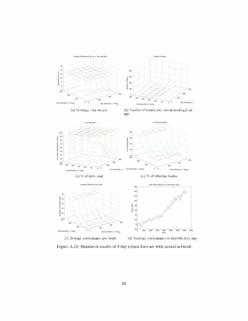
0
200
400
600
0
100
200
3004
6
8
10
12
14
16
Buy threshold: y > thetab
Strategy Performance % p.a. vs. buy-and-hold
Sell threshold: y < thetas
Per
form
ance
% p
.a.
(a) Strategy returns p.a.
0
200
400
600
050100
150200250
3000
100
200
300
400
Buy threshold: y >
Number of trades
Sell threshold: y < thetas
Num
ber
of t
rade
s
(b) Number of trades with corresponding strat-egy
0
200
400
600
05010015020025030020
30
40
50
60
70
80
90
100
Buy threshold: y > th
% of long days
Sell threshold: y < thetas
% o
f da
ys lo
ng p
ositi
on is
tak
en
(c) % of days long
0
200
400
600
0
100
200
30020
40
60
80
100
Buy threshold: y > thetab
% of winning trades
Sell threshold: y < thetas
% o
f w
inni
ng t
rade
s
(d) % of winning trades
0
200
400
600
0
100
200
3000
10
20
30
40
50
Buy threshold: y > thetab
Average Performance per trade
Sell threshold: y < thetas
Ave
rage
% r
etur
n pe
r tr
ade
(e) Average performance per trade
0 500 1000 1500 2000 2500 3000 3500 4000-20
0
20
40
60
80
100
120
140
160
Days
Ret
urn
(log)
Index Return (black) vs. Fund Return (red)
(f) Strategy performance as hypothetical fund
Figure A.15: Simulated results of 3-day return forecast with neural network
53

0 500 1000 1500 2000 2500 3000 3500-50
-40
-30
-20
-10
0
10
20
30
Days
Ret
urn
(log)
Index Return (black) vs. Fund Return (red)
(a) Fund performance
-35 -30 -25 -20 -15 -10 -5 0 5 100
0.1
0.2
0.3
0.4
0.5
0.6
0.7
0.8
0.9
1Trade Performance %
% performance per trade
Num
ber
of c
ases
(b) Trade histogram
Figure A.16: Simulated results of 3-day return forecast with neural network -out of sample application
54
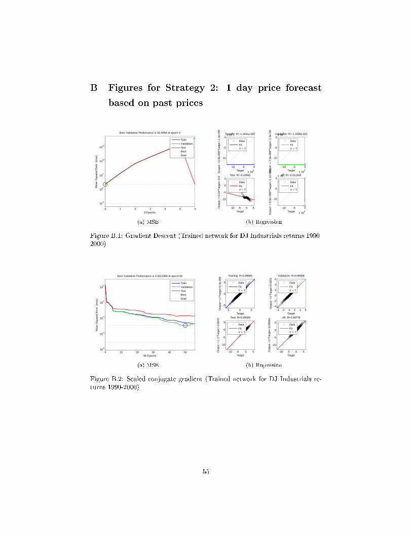
B Figures for Strategy 2: 1 day price forecast
based on past prices
0 1 2 3 4 5 6
10-5
100
105
1010
1015
Best Validation Performance is 81.6358 at epoch 0
Mea
n S
quar
ed E
rror
(m
se)
6 Epochs
Train
Validation
TestBest
Goal
(a) MSE
-10 -5 0
x 108
-10
-5
0x 10
8
Target
Out
put~
=2.
8e-0
09*T
arge
t+-1
.3e+
009
Training: R=-1.3441e-020
Data
FitY = T
-10 -5 0
x 108
-10
-5
0x 10
8
Target
Out
put~
=-7
.9e-
008*
Tar
get+
-1.3
e+00
9
Validation: R=-1.1936e-021
Data
FitY = T
-10 -5 0 5
-10
-5
0
5
Target
Out
put~
=-0
.24*
Tar
get+
-8.8
Test: R=-0.43562
Data
FitY = T
-10 -5 0
x 108
-10
-5
0x 10
8
Target
Out
put~
=-5
.6e+
006*
Tar
get+
-1.1
e+00
9
All: R=-0.011949
Data
FitY = T
(b) Regression
Figure B.1: Gradient Descent (Trained network for DJ Industrials returns 1990-2000)
0 10 20 30 40 5010
-6
10-4
10-2
100
102
Best Validation Performance is 0.0012369 at epoch 50
Mea
n S
quar
ed E
rror
(m
se)
56 Epochs
Train
Validation
TestBest
Goal
(a) MSE
-5 0 5
-5
0
5
Target
Out
put~
=1*
Tar
get+
3.4e
-005
Training: R=0.99905
Data
FitY = T
-4 -2 0 2 4 6-4
-2
0
2
4
6
Target
Out
put~
=1*
Tar
get+
0.00
21
Validation: R=0.99908
Data
FitY = T
-10 -5 0 5
-10
-5
0
5
Target
Out
put~
=1.
1*T
arge
t+-0
.004
3 Test: R=0.99309
Data
FitY = T
-10 -5 0 5
-10
-5
0
5
Target
Out
put~
=1*
Tar
get+
-0.0
0094
All: R=0.99778
Data
FitY = T
(b) Regression
Figure B.2: Scaled conjugate gradient (Trained network for DJ Industrials re-turns 1990-2000)
55
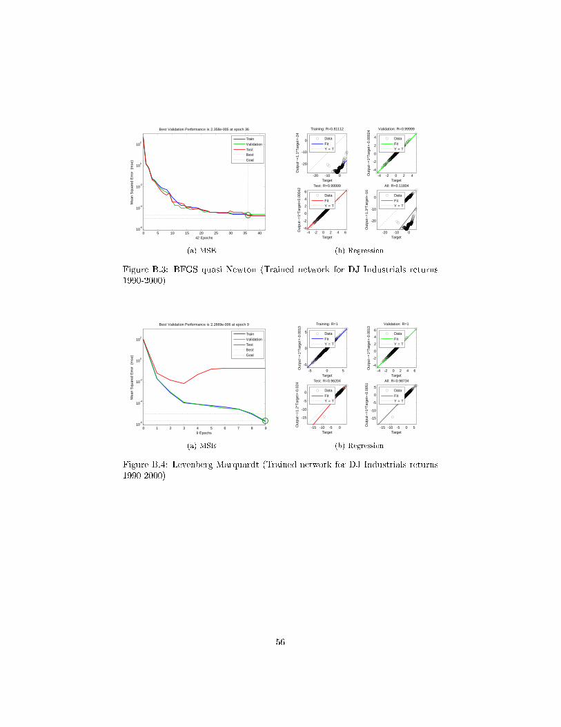
0 5 10 15 20 25 30 35 4010
-6
10-4
10-2
100
102
Best Validation Performance is 2.358e-005 at epoch 36M
ean
Squ
ared
Err
or
(mse
)
42 Epochs
Train
Validation
TestBest
Goal
(a) MSE
-20 -10 0
-20
-10
0
Target
Out
put~
=1.
1*T
arge
t+-2
4
Training: R=0.81112
Data
FitY = T
-4 -2 0 2 4
-4
-2
0
2
4
Target
Out
put~
=1*
Tar
get+
-0.0
0024
Validation: R=0.99999
Data
FitY = T
-4 -2 0 2 4 6-4
-2
0
2
4
6
Target
Out
put~
=1*
Tar
get+
0.00
042
Test: R=0.99999
Data
FitY = T
-20 -10 0
-20
-10
0
Target
Out
put~
=1.
3*T
arge
t+-1
6
All: R=0.11804
Data
FitY = T
(b) Regression
Figure B.3: BFGS quasi Newton (Trained network for DJ Industrials returns1990-2000)
0 1 2 3 4 5 6 7 8 910
-6
10-4
10-2
100
102
Best Validation Performance is 2.2669e-006 at epoch 9
Mea
n S
quar
ed E
rror
(m
se)
9 Epochs
Train
Validation
TestBest
Goal
(a) MSE
-5 0 5
-5
0
5
Target
Out
put~
=1*
Tar
get+
-0.0
013
Training: R=1
Data
FitY = T
-4 -2 0 2 4 6
-4
-2
0
2
4
6
Target
Out
put~
=1*
Tar
get+
-0.0
013
Validation: R=1
Data
FitY = T
-15 -10 -5 0
-15
-10
-5
0
Target
Out
put~
=1.
2*T
arge
t+-0
.024
Test: R=0.96204
Data
FitY = T
-15 -10 -5 0 5
-15
-10
-5
0
5
Target
Out
put~
=1*
Tar
get+
-0.0
051
All: R=0.98734
Data
FitY = T
(b) Regression
Figure B.4: Levenberg-Marquardt (Trained network for DJ Industrials returns1990-2000)
56

0 1 2 3 4 5 6 7 8
10-5
100
105
Best Validation Performance is 7.2872e-008 at epoch 8M
ean
Squ
ared
Err
or
(mse
)
8 Epochs
Train
Validation
TestBest
Goal
(a) MSE
-10 -5 0 5-10
-5
0
5
Target
Out
put~
=1*
Tar
get+
3.9e
-007
Training: R=1
Data
FitY = T
-4 -2 0 2 4
-4
-2
0
2
4
Target
Out
put~
=1*
Tar
get+
-2.2
e-00
7 Validation: R=1
Data
FitY = T
-4 -2 0 2 4 6-4
-2
0
2
4
6
Target
Out
put~
=1*
Tar
get+
2.9e
-009
Test: R=1
Data
FitY = T
-10 -5 0 5-10
-5
0
5
Target
Out
put~
=1*
Tar
get+
2.4e
-007
All: R=1
Data
FitY = T
(b) Regression
Figure B.5: Bayesian Regularization (Trained network for DJ Industrials returns1990-2000)
0 10 20 30 40 50 60 70 80 90 10010
-6
10-4
10-2
100
102
Best Validation Performance is 0.0012437 at epoch 99
Mea
n S
quar
ed E
rror
(m
se)
100 Epochs
Train
Validation
TestBest
Goal
(a) MSE
-5 0 5
-5
0
5
Target
Out
put~
=1*
Tar
get+
0.00
14
Training: R=0.99939
Data
FitY = T
-4 -2 0 2 4-4
-2
0
2
4
Target
Out
put~
=1*
Tar
get+
0.00
17
Validation: R=0.99935
Data
FitY = T
-10 -5 0 5-10
-5
0
5
Target
Out
put~
=1*
Tar
get+
0.00
1
Test: R=0.9991
Data
FitY = T
-10 -5 0 5-10
-5
0
5
Target
Out
put~
=1*
Tar
get+
0.00
13
All: R=0.99933
Data
FitY = T
(b) Regression
Figure B.6: Resilient Backpropagation (Trained network for DJ Industrials re-turns 1990-2000)
57

0 0.5 1 1.5 2 2.5 310
-6
10-4
10-2
100
102
Best Validation Performance is 0.26261 at epoch 2M
ean
Squ
ared
Err
or
(mse
)
3 Epochs
Train
Validation
TestBest
Goal
(a) MSE
-10 0 10 20-10
0
10
20
Target
Out
put~
=1.
9*T
arge
t+17
Training: R=0.98111
Data
FitY = T
-8 -6 -4 -2 0 2 4
-8
-6
-4
-2
0
2
4
Target
Out
put~
=0.
97*T
arge
t+-0
.034
Validation: R=0.88338
Data
FitY = T
-2 0 2 4
-2
0
2
4
Target
Out
put~
=1*
Tar
get+
-0.1
1
Test: R=0.88642
Data
FitY = T
-10 0 10 20-10
0
10
20
Target
Out
put~
=1.
7*T
arge
t+12
All: R=0.20661
Data
FitY = T
(b) Regression
Figure B.7: Conjugate Gradient with Powell/Beale Restarts (Trained networkfor DJ Industrials returns 1990-2000)
0 5 10 15 20 25 3010
-6
10-4
10-2
100
102
Best Validation Performance is 0.0058548 at epoch 31
Mea
n S
quar
ed E
rror
(m
se)
32 Epochs
Train
Validation
TestBest
Goal
(a) MSE
-10 0 10-10
0
10
Target
Out
put~
=0.
27*T
arge
t+17
Training: R=0.1712
Data
FitY = T
-2 0 2 4
-2
0
2
4
Target
Out
put~
=0.
98*T
arge
t+-0
.005
7 Validation: R=0.99679
Data
FitY = T
-4 -2 0 2
-4
-2
0
2
Target
Out
put~
=1*
Tar
get+
0.00
047
Test: R=0.99917
Data
FitY = T
-10 0 10-10
0
10
Target
Out
put~
=0.
44*T
arge
t+12
All: R=0.056121
Data
FitY = T
(b) Regression
Figure B.8: Fletcher-Powell Conjugate Gradient (Trained network for DJ In-dustrials returns 1990-2000)
58

0 5 10 15 20 25 30 35 4010
-6
10-4
10-2
100
102
Best Validation Performance is 0.0022844 at epoch 38M
ean
Squ
ared
Err
or
(mse
)
44 Epochs
Train
Validation
TestBest
Goal
(a) MSE
-15 -10 -5 0 5
-15
-10
-5
0
5
Target
Out
put~
=-0
.5*T
arge
t+-1
6
Training: R=-0.45695
Data
FitY = T
-4 -2 0 2 4
-4
-2
0
2
4
Target
Out
put~
=1*
Tar
get+
0.00
03
Validation: R=0.99849
Data
FitY = T
-10 -5 0 5-10
-5
0
5
Target
Out
put~
=0.
97*T
arge
t+-0
.008
2 Test: R=0.99781
Data
FitY = T
-15 -10 -5 0 5
-15
-10
-5
0
5
Target
Out
put~
=0.
11*T
arge
t+-1
1
All: R=0.014181
Data
FitY = T
(b) Regression
Figure B.9: Polak-Ribiére Conjugate Gradient (Trained network for DJ Indus-trials returns 1990-2000)
0 5 10 15 20 2510
-6
10-4
10-2
100
102
Best Validation Performance is 0.041082 at epoch 20
Mea
n S
quar
ed E
rror
(m
se)
26 Epochs
Train
Validation
TestBest
Goal
(a) MSE
-20 -10 0-20
-10
0
Target
Out
put~
=-0
.83*
Tar
get+
-16
Training: R=-0.65919
Data
FitY = T
-10 -5 0 5-10
-5
0
5
Target
Out
put~
=0.
93*T
arge
t+0.
0075
Validation: R=0.9819
Data
FitY = T
-8 -6 -4 -2 0 2
-8
-6
-4
-2
0
2
Target
Out
put~
=0.
96*T
arge
t+-0
.014
Test: R=0.98957
Data
FitY = T
-20 -10 0-20
-10
0
Target
Out
put~
=-0
.44*
Tar
get+
-12
All: R=-0.057579
Data
FitY = T
(b) Regression
Figure B.10: One Step Secant (Trained network for DJ Industrials returns 1990-2000)
59

0 10 20 30 40 50 60 70 80 90 10010
-6
10-4
10-2
100
102
Best Validation Performance is 0.014593 at epoch 100M
ean
Squ
ared
Err
or
(mse
)
100 Epochs
Train
Validation
TestBest
Goal
(a) MSE
-10 -5 0 5-10
-5
0
5
Target
Out
put~
=0.
96*T
arge
t+0.
0039
Training: R=0.9914
Data
FitY = T
-5 0 5
-5
0
5
Target
Out
put~
=0.
99*T
arge
t+-0
.003
1 Validation: R=0.99384
Data
FitY = T
-4 -2 0 2 4-4
-2
0
2
4
Target
Out
put~
=0.
98*T
arge
t+0.
0046
Test: R=0.99562
Data
FitY = T
-10 -5 0 5-10
-5
0
5
Target
Out
put~
=0.
97*T
arge
t+0.
0027
All: R=0.99234
Data
FitY = T
(b) Regression
Figure B.11: Variable Learning Rate Gradient Descent (Trained network for DJIndustrials returns 1990-2000)
0 1 2 3 4 5 6
10-5
100
105
Best Validation Performance is 72.2622 at epoch 0
Mea
n S
quar
ed E
rror
(m
se)
6 Epochs
Train
Validation
TestBest
Goal
(a) MSE
0 200 400 600 8000
200
400
600
800
TargetOut
put~
=0.
016*
Tar
get+
9.9e
+00
2
Training: R=0.23461
Data
FitY = T
0 200 400 600 8000
200
400
600
800
Target
Out
put~
=0.
19*T
arge
t+9.
9e+
002 Validation: R=0.43794
Data
FitY = T
-10 -5 0 5
-10
-5
0
5
Target
Out
put~
=1.
3*T
arge
t+-8
.4
Test: R=0.84663
Data
FitY = T
0 200 400 600 8000
200
400
600
800
Target
Out
put~
=1.
4*T
arge
t+8.
4e+
002 All: R=0.0040441
Data
FitY = T
(b) Regression
Figure B.12: Gradient Descent with Momentum (Trained network for DJ In-dustrials returns 1990-2000)
60

0 500 1000 1500 2000 2500 3000 3500 4000-15
-10
-5
0
5
10
(a) Gradient Descent with Momentum
0 500 1000 1500 2000 2500 3000 3500 4000-12
-10
-8
-6
-4
-2
0
2
4
6
8
(b) Bayesian Regularization
Figure B.13: Trained network for DJ Industrials returns 1990-2000, log returns,comparison between two methods
61
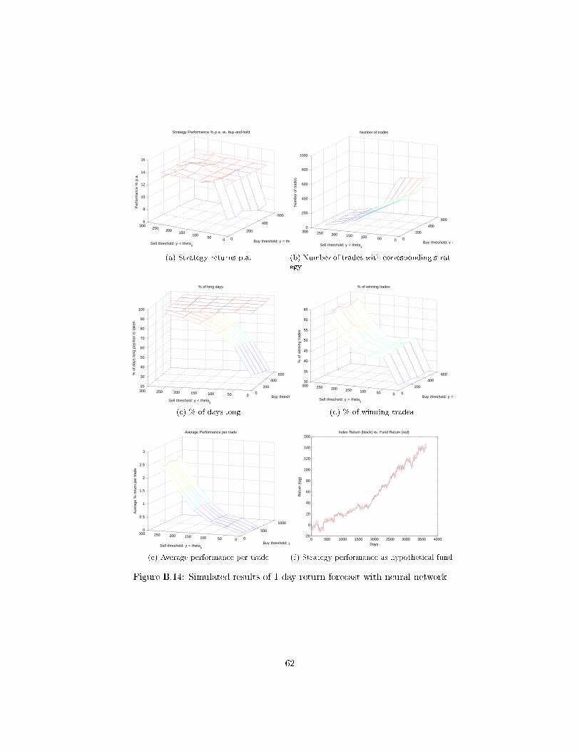
0
200
400
600
050
100150
200250
3006
8
10
12
14
16
Buy threshold: y > the
Strategy Performance % p.a. vs. buy-and-hold
Sell threshold: y < thetas
Per
form
ance
% p
.a.
(a) Strategy returns p.a.
0
200
400
600
0501001502002503000
200
400
600
800
1000
Buy threshold: y >
Number of trades
Sell threshold: y < thetas
Num
ber
of t
rade
s
(b) Number of trades with corresponding strat-egy
0
200
400
600
05010015020025030020
30
40
50
60
70
80
90
100
Buy thresho
% of long days
Sell threshold: y < thetas
% o
f da
ys lo
ng p
ositi
on is
tak
en
(c) % of days long
0
200
400
600
05010015020025030030
35
40
45
50
55
60
65
Buy threshold: y >
% of winning trades
Sell threshold: y < thetas
% o
f w
inni
ng t
rade
s
(d) % of winning trades
0
500
1000
0501001502002503000
0.5
1
1.5
2
2.5
3
Buy threshold: y
Average Performance per trade
Sell threshold: y < thetas
Ave
rage
% r
etur
n pe
r tr
ade
(e) Average performance per trade
0 500 1000 1500 2000 2500 3000 3500 4000-20
0
20
40
60
80
100
120
140
160
Days
Ret
urn
(log)
Index Return (black) vs. Fund Return (red)
(f) Strategy performance as hypothetical fund
Figure B.14: Simulated results of 1-day return forecast with neural network
62

C Figures for Strategy 3: forecast based on �-
nancial factors
0 1 2 3 4 5 6
100
1020
1040
1060
1080
10100
Best Validation Performance is 11799046.62 at epoch 0
Mea
n S
quar
ed E
rror
(m
se)
6 Epochs
Train
Validation
TestBest
Goal
(a) MSE
0 2 4 6 8 10 12 14
x 104
-1
-0.5
0
0.5
1
1.5
2x 10
4
(b) Output signal
Figure C.1: Gradient Descent (Trained network for DJ Industrials returns 1990-2000)
0 10 20 30 40 50 60 70 80 90 100
10-5
100
105
Best Validation Performance is 5839.9407 at epoch 97
Mea
n S
quar
ed E
rror
(m
se)
100 Epochs
Train
Validation
TestBest
Goal
(a) MSE
0 2 4 6 8 10 12 14
x 104
-5000
-4000
-3000
-2000
-1000
0
1000
(b) Network output
Figure C.2: Scaled conjugate gradient (Trained network for DJ Industrials re-turns 1990-2000)
63

0 5 10 15 20 25 30
10-5
100
105
Best Validation Performance is 357021.06 at epoch 32M
ean
Squ
ared
Err
or
(mse
)
32 Epochs
Train
Validation
TestBest
Goal
(a) MSE
0 2 4 6 8 10 12 14
x 104
-6000
-4000
-2000
0
2000
4000
6000
8000
10000
12000
(b) Network output
Figure C.3: BFGS quasi Newton (Trained network for DJ Industrials returns1990-2000)
0 5 10 15
10-5
100
105
1010
Best Validation Performance is 9632.4239 at epoch 9
Mea
n S
quar
ed E
rror
(m
se)
15 Epochs
Train
Validation
TestBest
Goal
(a) MSE
0 2 4 6 8 10 12 14
x 104
-15
-10
-5
0
5
10
15
20
(b) Network output
Figure C.4: Levenberg-Marquardt (Trained network for DJ Industrials returns1990-2000)
64

0 1 2 3 4 5 6 7 8 9 10 11
10-5
100
105
1010
Best Validation Performance is 50261301.5806 at epoch 8M
ean
Squ
ared
Err
or
(mse
)
11 Epochs
Train
Validation
TestBest
Goal
(a) MSE
0 2 4 6 8 10 12 14
x 104
-2
-1
0
1
2
3
4
5
6
7
8
(b) Network output
Figure C.5: Bayesian Regularization (Trained network for DJ Industrials returns1990-2000)
0 10 20 30 40 50 60 70 80 90 100
10-5
100
105
Best Validation Performance is 24210.8413 at epoch 100
Mea
n S
quar
ed E
rror
(m
se)
100 Epochs
Train
Validation
TestBest
Goal
(a) MSE
0 2 4 6 8 10 12 14
x 104
-14000
-12000
-10000
-8000
-6000
-4000
-2000
0
2000
4000
(b) Network output
Figure C.6: Resilient Backpropagation (Trained network for DJ Industrials re-turns 1990-2000)
65

0 5 10 15
10-5
100
105
1010
Best Validation Performance is 2732.7463 at epoch 14M
ean
Squ
ared
Err
or
(mse
)
15 Epochs
Train
Validation
TestBest
Goal
(a) MSE
0 2 4 6 8 10 12 14
x 104
-4000
-3000
-2000
-1000
0
1000
2000
(b) Regression
Figure C.7: Conjugate Gradient with Powell/Beale Restarts (Trained networkfor DJ Industrials returns 1990-2000)
0 5 10 15 20 25 30 35 40 45 50
10-5
100
105
Best Validation Performance is 16111.5459 at epoch 51
Mea
n S
quar
ed E
rror
(m
se)
52 Epochs
Train
Validation
TestBest
Goal
(a) MSE
0 2 4 6 8 10 12 14
x 104
-2000
0
2000
4000
6000
8000
10000
12000
14000
16000
(b) Network output
Figure C.8: Fletcher-Powell Conjugate Gradient (Trained network for DJ In-dustrials returns 1990-2000)
66

0 5 10 15 20 25 30 35 40 45 50
10-5
100
105
Best Validation Performance is 16111.5459 at epoch 51M
ean
Squ
ared
Err
or
(mse
)
52 Epochs
Train
Validation
TestBest
Goal
(a) MSE
0 2 4 6 8 10 12 14
x 104
-2000
-1000
0
1000
2000
3000
4000
5000
6000
7000
(b) Network output
Figure C.9: Polak-Ribiére Conjugate Gradient (Trained network for DJ Indus-trials returns 1990-2000)
0 10 20 30 40 50 60 70 80 90 10010
-6
10-4
10-2
100
102
104
106
Best Validation Performance is 15129.8116 at epoch 100
Mea
n S
quar
ed E
rror
(m
se)
100 Epochs
Train
Validation
TestBest
Goal
(a) MSE
0 2 4 6 8 10 12 14
x 104
-3000
-2500
-2000
-1500
-1000
-500
0
500
1000
(b) Network output
Figure C.10: One Step Secant (Trained network for DJ Industrials returns 1990-2000)
67

0 10 20 30 40 50 60 70 80 90 10010
-6
10-4
10-2
100
102
Best Validation Performance is 0.014593 at epoch 100M
ean
Squ
ared
Err
or
(mse
)
100 Epochs
Train
Validation
TestBest
Goal
(a) MSE
-10 -5 0 5-10
-5
0
5
Target
Out
put~
=0.
96*T
arge
t+0.
0039
Training: R=0.9914
Data
FitY = T
-5 0 5
-5
0
5
Target
Out
put~
=0.
99*T
arge
t+-0
.003
1 Validation: R=0.99384
Data
FitY = T
-4 -2 0 2 4-4
-2
0
2
4
Target
Out
put~
=0.
98*T
arge
t+0.
0046
Test: R=0.99562
Data
FitY = T
-10 -5 0 5-10
-5
0
5
Target
Out
put~
=0.
97*T
arge
t+0.
0027
All: R=0.99234
Data
FitY = T
(b) Regression
Figure C.11: Variable Learning Rate Gradient Descent (Trained network for DJIndustrials returns 1990-2000)
0 1 2 3 4 5 6
100
1020
1040
1060
1080
10100
Best Validation Performance is 1962658983.6456 at epoch 0
Mea
n S
quar
ed E
rror
(m
se)
6 Epochs
Train
Validation
TestBest
Goal
(a) MSE
0 2 4 6 8 10 12 14
x 104
-4.8
-4.6
-4.4
-4.2
-4
-3.8
-3.6
-3.4
-3.2x 10
4
(b) Network output
Figure C.12: Gradient Descent with Momentum (Trained network for DJ In-dustrials returns 1990-2000)
68

0 1000 2000 3000 4000 5000 6000 7000 8000-50
0
50
100
150
200
250
300
350
Days
Ret
urn
(log)
Index Return (black) vs. Fund Return (red)
(a) Simulated fund performance (red) vs. buy-and-hold performance
0 1000 2000 3000 4000 5000 6000 7000 80000
10
20
30
40
50
60
70
80
90
100
Days
# of
inve
stm
ents
Amount of investments in index (black) vs. Fund Return (red)
(b) Amount of long positions in di�erent stocksof the S&P100
-100 -50 0 500
2
4
6
8
10
12
14
16
18Strategy Performance p.a. %
% p.a.
Num
ber
of c
ases
(c) Histogram with di�erent stocks - outperfor-mance of strategy
0 200 400 600 800 1000 1200 1400 1600 18000
5
10
15
20
25
30
35
40
45
50Number of trades
Number of trades
Num
ber
of c
ases
(d) Histogram showing number of trades witheach stock
36 38 40 42 44 46 48 50 520
2
4
6
8
10
12
14
16% of winning trades
% of winning trades
Num
ber
of c
ases
(e) Histogram with % of winning trades
-60 -50 -40 -30 -20 -10 0 10 20 300
5
10
15
20
25Strategy Outperformance %
Outperformance % p.a.
Num
ber
of c
ases
(f) Strategy outperformance
Figure C.13: Strategy results with �nancial factors as input neurons
69

D Program Listings
D.1 Neural Network
D.1.1 Neural Network Main program (training) [training.m]
1 clear;
2 clear n;
3 method =4; % 0=sigmoid , 1=tanh , 2=linear , 4= Newton method
4 %output node always uses linear
5
6 learningRate =0.15;
7 normalize =0;
8 first_input =1;
9 last_output =8;
10
11 for x=1:8
12 n(x)=NeuronNewton;
13 end
14
15 % node connections
16 %n=n.addConnection (3, 1, 1.2, -0.1); % target , origin , weight ,
bias
17 %n=n.addConnection (3, 2, 1.25 , -0.1);
18 %n=n.addConnection (4, 1, 1.3, -0.15);
19 %n=n.addConnection (4, 2, -0.1,-0.15);
20 %n=n.addConnection (5, 3, -0.1, 0.05);
21 %n=n.addConnection (5, 4, 0.2, 0.05);
22
23 % Nicolas Coursework
24 %n=n.addConnection (3, 1, 0.23, 0.0); % target , origin , weight ,
bias
25 %n=n.addConnection (4, 2, 0.14, 0.0);
26 %n=n.addConnection (5, 2, 0.3, 0.0);
27 %n=n.addConnection (5, 1, -0.35, 0.0);
28 %n=n.addConnection (6, 3, 0.1, 0.0);
29 %n=n.addConnection (6, 4, -0.2, 0.0);
30 %n=n.addConnection (6, 5, -0.4, 0.0);
31 %n=n.addConnection (6, 1, 0.3, 0.0);
32
33 % Irati coursework
34 n=n.addConnection (3, 1, 0.14, 0.0); % target , origin , weight ,
bias
35 n=n.addConnection (4, 2, -0.3, 0.0);
36 n=n.addConnection (5, 2, -0.1, 0.0);
37 n=n.addConnection (5, 1, 0.5, 0.0);
70

38 n=n.addConnection (6, 3, 0.4, 0.0);
39 n=n.addConnection (6, 4, -0.4, 0.0);
40 n=n.addConnection (6, 5, -0.15, 0.0);
41 n=n.addConnection (6, 1, -0.23, 0.0);
42
43
44 % define structure (type =0: input node , type =1: hidden node , type
=2: output
45 % node
46 n(1).type =0;
47 n(2).type =0;
48 n(3).type =1;
49 n(4).type =1;
50 n(5).type =1;
51 n(6).type =2;
52
53
54
55
56 for i=1:1
57
58 % input nodes
59 n(1).output =1;%round(rand (1)); %input values for input nodes
60 n(2).output =0;%round(rand (1));
61
62 endvalue=xor( n(1).output , n(2).output ); %output node correct
result
63
64
65 % generate output for forward propagation
66 n(3)=n(3).getOutput(n,0);
67 n(4)=n(4).getOutput(n,0);
68 n(5)=n(5).getOutput(n,0);
69 n(6)=n(6).getOutput(n,2);
70
71
72 % backward propagation
73 n=n.backProp(6,endvalue ,2);
74 n=n.backProp(5,endvalue ,0);
75 n=n.backProp(4,endvalue ,0);
76 n=n.backProp(3,endvalue ,0);
77
78 if method <4 % MPL method
79 [n]=n.weightUpdate (6, learningRate);
80 [n]=n.weightUpdate (5, learningRate);
81 [n]=n.weightUpdate (4, learningRate);
71

82 [n]=n.weightUpdate (3, learningRate);
83
84 elseif method ==4 % Newton method
85 % weight updating
86 [n,j]=n.weightUpdate (6,j);
87 [n,j]=n.weightUpdate (5,j);
88 [n,j]=n.weightUpdate (4,j);
89 [n,j]=n.weightUpdate (3,j);
90
91
92 %calculate hessian
93 H=j*j';
94 h=1/H;
95 %update weights
96 [n]=n.weightUpdateNewton (6,h);
97 [n]=n.weightUpdateNewton (5,h);
98 [n]=n.weightUpdateNewton (4,h);
99 [n]=n.weightUpdateNewton (3,h);
100
101 end
102
103
104 %result(i)=round(n(5).output)== endvalue;
105
106 end
107
108 for nx=3:6
109 node=nx %output result
110 n(nx).inputweight
111 end
112
113
114 %figure (1)
115 %plot((n(6).deltaHistory).^2)
116 %figure (2)
117 %plot (result);
D.1.2 Neuron Class [Neuron.m]
1 classdef Neuron
2 %Neuron for neuronal network
3 %
4
5 properties
6 bias
72

7 inputweight
8 connections % backward looking connections
9 followers % forward looking connections
10 type
11 output
12 beta
13 delta
14 previous_delta
15 delta_bias
16
17 deltaHistory
18 biasHistory
19 firstWeightHistory
20 end
21
22 methods
23 function [this]= getOutput(this ,neurons ,param)
24
25 this.output=this.bias;
26
27 for n=1: numel(this.connections)
28 this.output=this.output+this.inputweight(n)*
neurons(this.connections(n)).output;
29 end
30
31 if param ==0 this.output=sigmoid(this.
output); end
32 if param ==1 this.output=tanh_backprop(
this.output); end
33 if param ==2 this.output=this.output; end
34 if param ==3 this.output=tanh_backprop(
this.output); end
35 if param ==4 this.output=tanh_backprop(
this.output); end
36
37
38
39 end
40
41 function [neuron ]= addConnection(neuron ,target ,origin ,
weight ,bias)
42 neuron(target).connections(numel(neuron(target).
connections)+1)=origin;
43 neuron(target).inputweight(numel(neuron(target).
inputweight)+1)=weight;
44 neuron(target).bias (1)=bias;
73
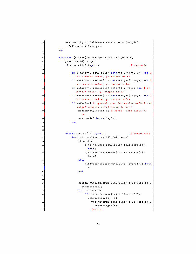
45 neuron(origin).followers(numel(neuron(origin).
followers)+1)=target;
46 end
47
48 function [neuron ]= backProp(neuron ,id,d,method)
49 y=neuron(id).output;
50 if neuron(id).type ==2 % end node
51
52 if method ==0 neuron(id).beta=(d-y)*y*(1-y); end %
d: correct value , y: output value
53 if method ==1 neuron(id).beta=(d-y)*(1-y*y); end %
d: correct value , y: output value
54 if method ==2 neuron(id).beta=(d-y)*(1); end % d:
correct value , y: output value
55 if method ==3 neuron(id).beta=(d-y)*(1-y*y); end %
d: correct value , y: output value
56 if method ==4 % special case for newton method and
output neuron , betaJ needs to be 1
57 neuron(id).betaJ =1; % outbut beta shoud be
one
58 neuron(id).beta=(d-y)*1;
59 end
60
61
62 elseif neuron(id).type ==1 % inner node
63 for f=1: numel(neuron(id).followers)
64 if method ==4
65 b (f)=neuron(neuron(id).followers(f)).
beta;
66 bj(f)=neuron(neuron(id).followers(f)).
betaJ;
67 else
68 b(f)=neuron(neuron(id).followers(f)).beta
;
69 end
70
71
72 search=numel(neuron(neuron(id).followers(f)).
connections);
73 for s=1: search
74 if neuron(neuron(id).followers(f)).
connections(s)==id
75 w(f)=neuron(neuron(id).followers(f)).
inputweight(s);
76 %break;
74

77 %w(f)=interp1 (neuron(neuron(id).
followers(f)).connections , neuron(
neuron(id).followers(f)).
inputweight , id, 'nearest '); % fwd
weight lookup
78 end
79 end
80
81
82
83 end
84 q=0;
85 qj=0;
86 for f=1: numel(neuron(id).followers)
87 q= q +w(f)*b (f);
88 if method ==4
89 qj=qj+w(f); % bj is not multiplied by the
beta
90 end
91 end
92 if method ==0 neuron(id).beta=(q)*y*(1-y); end
93 if method ==1 neuron(id).beta=(q)*(1-y*y); end
94 if method ==2 neuron(id).beta=(q)*(1); end
95 if method ==3 neuron(id).beta=(q)*(1-y*y); end
96 if method ==4 neuron(id).betaJ =(qj)*(1-y*y); % bj
is not multiplied by the beta
97 neuron(id).beta= (q) *(1-y*y);
98 end %Newton
99 end
100 neuron(id).deltaHistory(numel(neuron(id).deltaHistory
)+1)=(d-y)*(d-y);%neuron(id).beta;
101 %neuron(id).History(numel(neuron(id).biasHistory)+1)=
neuron(id).bias;
102 neuron(id).firstWeightHistory(numel(neuron(id).
firstWeightHistory)+1)=neuron(id).inputweight (1);
103 end
104
105
106
107 function [neuron ]= weightUpdate(neuron ,id,learningRate ,
method ,firstTake ,momentum)
108 neuron(id).delta_bias=neuron(id).beta*learningRate;
109 neuron(id).bias = 0;%neuron(id).bias + neuron(id).
delta_bias;
110 for n=1: numel(neuron(id).connections)
111 if method ==3
75

112 if firstTake ==true neuron(id).delta(n)=0;
113 neuron(id).delta(n);
114 end
115 neuron(id).delta(n) = neuron(id).delta(n) +
neuron(id).beta * learningRate * neuron(
neuron(id).connections(n)).output;
116 else
117 if firstTake ==true neuron(id).previous_delta(
n)=0; end
118 neuron(id).delta(n)=neuron(id).beta*
learningRate*neuron(neuron(id).connections(
n)).output;
119 neuron(id).inputweight(n) = neuron(id).
inputweight(n) + neuron(id).delta(n)*(1-
momentum) + momentum*neuron(id).
previous_delta(n);
120 end
121 end
122 neuron(id).previous_delta=neuron(id).delta;
123 end
124
125
126 function [neuron ]= batchUpdate(neuron ,id,learningRate)
127 neuron(id).delta_bias=neuron(id).beta*learningRate;
128 neuron(id).bias = 0;%neuron(id).bias + neuron(id).
delta_bias;
129 for n=1: numel(neuron(id).connections)
130 neuron(id).delta(n);
131 neuron(id).inputweight(n) = neuron(id).
inputweight(n) + neuron(id).delta(n);
132 neuron(id).delta(n)=0;
133 end
134 end
135 end
136 end
D.1.3 Neuron Class [NeuronNewton.m]
1 classdef NeuronNewton < Neuron % inherit Neuron class
2 %Neuron for neuronal network for quasi -Newton method
3 %
4
5 properties
6 betaJ
7 end
76
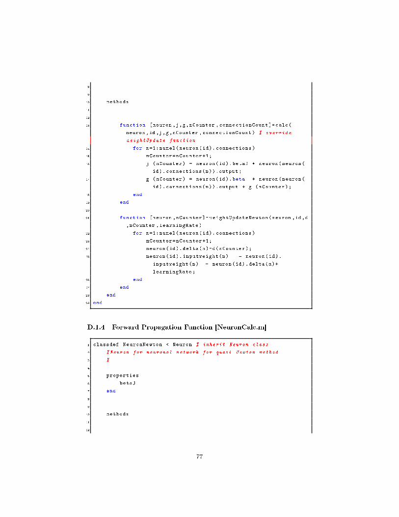
8
9
10 methods
11
12
13 function [neuron ,j,g,nCounter ,connectionCount ]=calc(
neuron ,id,j,g,nCounter ,connectionCount) % override
weightUpdate function
14 for n=1: numel(neuron(id).connections)
15 nCounter=nCounter +1;
16 j (nCounter) = neuron(id).betaJ * neuron(neuron(
id).connections(n)).output;
17 g (nCounter) = neuron(id).beta * neuron(neuron(
id).connections(n)).output + g (nCounter);
18 end
19 end
20
21 function [neuron ,nCounter ]= weightUpdateNewton(neuron ,id,d
,nCounter ,learningRate)
22 for n=1: numel(neuron(id).connections)
23 nCounter=nCounter +1;
24 neuron(id).delta(n)=d(nCounter);
25 neuron(id).inputweight(n) = neuron(id).
inputweight(n) + neuron(id).delta(n)*
learningRate;
26 end
27 end
28 end
29 end
D.1.4 Forward Propagation Function [NeuronCalc.m]
1 classdef NeuronNewton < Neuron % inherit Neuron class
2 %Neuron for neuronal network for quasi -Newton method
3 %
4
5 properties
6 betaJ
7 end
8
9
10 methods
11
12
77

13 function [neuron ,j,g,nCounter ,connectionCount ]=calc(
neuron ,id,j,g,nCounter ,connectionCount) % override
weightUpdate function
14 for n=1: numel(neuron(id).connections)
15 nCounter=nCounter +1;
16 j (nCounter) = neuron(id).betaJ * neuron(neuron(
id).connections(n)).output;
17 g (nCounter) = neuron(id).beta * neuron(neuron(
id).connections(n)).output + g (nCounter);
18 end
19 end
20
21 function [neuron ,nCounter ]= weightUpdateNewton(neuron ,id,d
,nCounter ,learningRate)
22 for n=1: numel(neuron(id).connections)
23 nCounter=nCounter +1;
24 neuron(id).delta(n)=d(nCounter);
25 neuron(id).inputweight(n) = neuron(id).
inputweight(n) + neuron(id).delta(n)*
learningRate;
26 end
27 end
28 end
29 end
D.1.5 Sigmoid function [sigmoid.m]
1 function [ y ] = sigmoid( x )
2 % Outputs the sigmoid function s(x)
3
4 y=1./(1+ exp(-(x)));
5 %y=1 -2./( exp (2*x)+1);
6
7 end
D.1.6 Neural Network Training with Toolbox [train_matlab1.m]
1 % Solve an Input -Output Fitting problem with a Neural Network
2 % Script generated by NFTOOL
3 %
4 % This script assumes these variables are defined:
5 %
6 % houseInputs - input data.
78

7 % houseTargets - target data.
8 clear all;
9
10 [p,t,series_n ]= createInputOutput2; % create continous output
11
12 %net = newff(p,t,5,{},'traingd '); % gradient descent
13 %net = newff(p,t,5,{},'trainscg ');% Scaled Conjugate Gradient
14 %net = newff(p,t,5,{},'trainbfg '); % BFGS Quasi -Newton
15
16 %net = newff(p,t,5,{},'trainlm '); % Levenberg -Marquardt
17 net = newff(p,t,5,{},'trainbr '); % Bayesian Regularization
18 %net = newff(p,t,5,{},'trainrp '); % Resilient Backpropagation
19 %net = newff(p,t,5,{},'traincgb ');% Conjugate Gradient with
Powell/Beale Restarts
20 %net = newff(p,t,5,{},'traincgf ');% Fletcher -Powell Conjugate
Gradient
21 %net = newff(p,t,5,{},'traincgp ');% Polak -Ribiére Conjugate
Gradient
22 %net = newff(p,t,5,{},'trainoss ');% One Step Secant
23 %net = newff(p,t,5,{},'traingdx ');% Variable Learning Rate
Gradient Descent
24 %net = newff(p,t,5,{},'traingdm ');% Gradient Descent with
Momentum
25
26
27 net.divideFcn = 'dividerand ';
28
29 %net.trainParam.show = 50;
30 net.trainParam.lr = 0.1;
31 net.trainParam.epochs = 100;
32 net.trainParam.goal = 1e-5;
33 net.layers {1}. transferFcn = 'logsig ';
34 net.divideParam.trainRatio = 70/100;
35 net.divideParam.valRatio = 15/100;
36 net.divideParam.testRatio = 15/100;
37 %net.trainParam.showWindow =0;
38
39
40 [net ,tr]=train(net ,p,t);
41 %plotperform(tr);
42
43
44 figure (1);
45 plot(series_n (:,1),'b');
46 hold on;
47 plot(sim(net ,p(:,:)),'r');
79

48 hold off;
D.1.7 Neural Network Training with Toolbox [train_matlab3.m]
1 % Solve an Input -Output Fitting problem with a Neural Network
2 % Script generated by NFTOOL
3 %
4 % This script assumes these variables are defined:
5 %
6 % houseInputs - input data.
7 % houseTargets - target data.
8
9 %{
10 clear all;
11
12 mode =47;
13 [x1 ,xs,x2 ,y1,ys ,y2,z1,zs,z2,n1 ,ns,n2 ,c,ms , strategy , filename ,
sheetname , total_calculations] = trading_presets(mode);
14
15 TS=TimeSeries;
16 TS=load_time_series(TS, filename , sheetname , n1,ns,n2 ,c,ms); %
load time serie
17
18
19 %}
20
21 % put together training matrixes
22 a=1;
23 x=0;
24 for n=4:102
25 for i=10:TS(n).number_of_returns -31
26 % data check
27 if ~isnan (sum(TS(n).returns_normalized(i:i+1))) && ~
isnan (sum(TS(n).second(i-a:i))) && ~isnan (sum(TS(
n).third(i-a:i))) && ~isnan (sum(TS(n).prices(i-a:i
)))
28 x=x+1;
29 % p=inputs
30 p(1,x)=TS(n).second(i)/TS(n).second(i-a) -1;
31 p(2,x)=TS(n).third(i)/TS(n).second(i-a) -1;
32 p(3,x)=TS(n).fourth(i)/TS(n).second(i-a) -1;
33 % t=targets or outputs
34 t(x)=TS(n).returns_normalized(i+a)/TS(n).
returns_normalized(i) -1;
35 if mod(x ,10000) ==0
80

36 complete_est=x/700000*100
37 end;
38 end
39
40 end
41 end
42
43
44 %net = newff(p,t,10,{},'traingd '); % gradient descent
45 %net = newff(p,t,10,{},'trainscg ');% Scaled Conjugate Gradient
46 %net = newff(p,t,10,{},'trainbfg '); % BFGS Quasi -Newton
47
48 %net = newff(p,t,10,{},'trainlm '); % Levenberg -Marquardt
49 %net = newff(p,t,10,{},'trainbr '); % Bayesian Regularization
50 %net = newff(p,t,10,{},'trainrp '); % Resilient Backpropagation
51 %net = newff(p,t,10,{},'traincgb ');% Conjugate Gradient with
Powell/Beale Restarts
52 %net = newff(p,t,10,{},'traincgf ');% Fletcher -Powell Conjugate
Gradient
53 %net = newff(p,t,10,{},'traincgp ');% Polak -Ribiére Conjugate
Gradient
54 %net = newff(p,t,10,{},'trainoss ');% One Step Secant
55 %net = newff(p,t,10,{},'traingdx ');% Variable Learning Rate
Gradient Descent
56 net = newff(p,t,10,{},'traingdm ');% Gradient Descent with
Momentum
57
58
59 net.divideFcn = 'dividerand ';
60
61 %net.trainParam.show = 50;
62 net.trainParam.lr = 0.1;
63 net.trainParam.epochs = 100;
64 net.trainParam.goal = 1e-5;
65 net.layers {1}. transferFcn = 'logsig ';
66 net.divideParam.trainRatio = 70/100;
67 net.divideParam.valRatio = 15/100;
68 net.divideParam.testRatio = 15/100;
69 %net.trainParam.showWindow =0;
70
71
72 [net ,tr]=train(net ,p,t);
73 %plotperform(tr);
74
75
76 figure (1);
81

77 %plot(series_n (:,1) ,'b');
78 %hold on;
79 plot(sim(net ,p(:,:)),'r');
80 hold off;
D.2 Trading Simulator
D.2.1 Main program [main.m]
1 clear;
2 clear classes; nn=0;
3
4 %% Objects
5 % TS: time series data
6 % F: Total Fund returns and Index returns on daily basis
7 % G: strategy: Subclass of trade_generator which communicates
with the strategy
8 % T: trades
9 % A: analysis of a specific scenario (i.e. summing up the trades)
10 % O: optimum and graphs
11 %% Parameters
12
13 %mode =1; % Buying after selloff after several months , then
profittaking
14 %mode =5; % Buying after selloff after several months , x day sell
15 %mode =2; % Buying after selloff after several days , then
profittaking
16 %mode =21; % Buying after selloff after several days , then
profittaking one case
17
18 %mode =3; % Buying after selloff after several months , buying
after days
19
20 %mode =4; % Buying after selloff after several days , then
profittaking SMI
21 %mode =6; % Payout ratio *
22
23 %mode =8; % Stop loss and buy after reaching x day low *
24 %mode =9; % Special Stop loss and buy after reaching x day low
25 %mode =10; % Analyst recommendations
26 %mode =11; % Analyst recommendations test
27 %mode =19; % Special stop strategy: dynamic stop , buy after price >
sell price
28
29 %mode =29; % Coppock curve
82

30
31 %mode =30; % Moving average *
32
33 %mode =40; load('trained -5 inputNeurons.mat '); % Neural Network 1
34 %mode =41; load('trained -5 inputNeurons.mat '); % Neural Network 1
35
36 %mode =42; load('trained -10 inputNeurons -5d-5t.mat '); % Neural
Network 1
37 %mode =43; load('trained -10 inputNeurons -5d-5t.mat '); % Neural
Network 1
38
39 %mode =44; load('net2.mat '); nn=net; % Neural Network 2
40 %mode =45; load('net2.mat '); nn=net; % Neural Network 2
41
42 %mode =46; load('net2b.mat '); nn=net; % Neural Network 2
43
44 mode =47; load('net3.mat'); nn=net; % Neural Network 3
45
46
47 %mode =101; % quick: Buying after selloff after several days , then
profittaking
48 %mode =1001; % SP100 , one case
49
50 %mode =9000; % testsheet
51
52 [x1 ,xs,x2 ,y1,ys ,y2,z1,zs,z2,n1 ,ns,n2 ,c,ms , strategy , filename ,
sheetname , total_calculations] = trading_presets(mode);
53
54 %% Start of main program
55
56 rf=2; % 2 pct risk free rate
57
58 graphmode =1; % 1: more than one
case
59 if x2-x1+y2-y1+z2 -z1+n2 -n1==0 graphmode =2 ; end % 2: analyze
only one case (2d histogram in analysis)
60 if n2-n1 >0
61 graphmode =3; % 3: more than one
case for various stocks (3d histogram)
62 if x2-x1+y2-y1+z2 -z1==0 graphmode =4; end % 4: analyze only
one case for various stocks (2d histogram in graph)
63 end
64
65 eta=Eta;
66 calc =0;
67 tic;
83
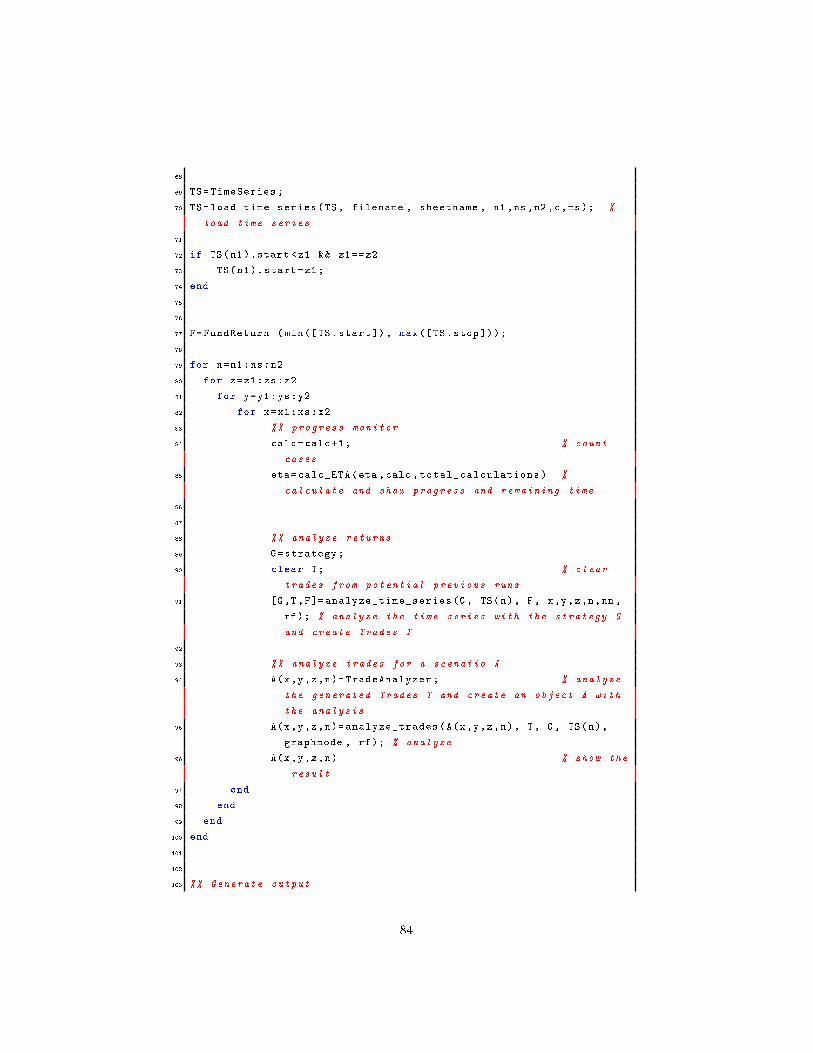
68
69 TS=TimeSeries;
70 TS=load_time_series(TS, filename , sheetname , n1,ns,n2 ,c,ms); %
load time series
71
72 if TS(n1).start <z1 && z1==z2
73 TS(n1).start=z1;
74 end
75
76
77 F=FundReturn (min([TS.start]), max([TS.stop]));
78
79 for n=n1:ns:n2
80 for z=z1:zs:z2
81 for y=y1:ys:y2
82 for x=x1:xs:x2
83 %% progress monitor
84 calc=calc +1; % count
cases
85 eta=calc_ETA(eta ,calc ,total_calculations) %
calculate and show progress and remaining time
86
87
88 %% analyze returns
89 G=strategy;
90 clear T; % clear
trades from potential previous runs
91 [G,T,F]= analyze_time_series(G, TS(n), F, x,y,z,n,nn,
rf); % analyze the time series with the strategy G
and create Trades T
92
93 %% analyze trades for a scenatio A
94 A(x,y,z,n)=TradeAnalyzer; % analyze
the generated Trades T and create an object A with
the analysis
95 A(x,y,z,n)=analyze_trades(A(x,y,z,n), T, G, TS(n),
graphmode , rf); % analyze
96 A(x,y,z,n) % show the
result
97 end
98 end
99 end
100 end
101
102
103 %% Generate output
84

104
105 if graphmode ==2 || graphmode ==4
106 lag=round ((TS(n).stop -TS(n).start)/10);
107 lag=1;
108 F=F.plotReturns (lag ,1);
109 end
110
111 O=TradeGraphs; % generate
the graphs and calculate the optimum in in object O
112 O=graph (O,A,G,x1,xs,x2,y1,ys,y2,z1 ,zs,z2 ,n1,ns,n2,graphmode ,G.
start);
113
114 if graphmode ==1
115 % calculate again trades for optimum and perform a wilcoxon
test on the
116 % best annaulized_return strategy
117 clear F;
118 F=FundReturn (min([TS.start]), max([TS.stop]));
119 G=strategy;
120 n=1;
121 G.start=(O.opt_z -1)+1; %
start analysis on day G.start
122 [G,T,F]= analyze_time_series(G, TS(n), F, O.opt_x ,O.opt_y ,O.
opt_z ,n,nn,rf);
123 disp ('Signrank test for avg performance per trade annaulized
is different to buy and hold return ');
124 [p,test]= signrank ([T.annualized_return],mean([A.
buy_hold_performance_pa ]))
125 if test ==1 && (mean([T.annualized_return ]) > mean([A.
buy_hold_performance_pa ]))
126 disp ('!!!!!!!!!!!!!!!!!! POTENTIAL STRATEGY FOUND
!!!!!!!!!!!!!!!!!! ');
127 end
128 lag=round ((TS(n).stop -TS(n).start)/10);
129 lag=1;
130 F=F.plotReturns(lag ,1);
131 end
D.2.2 TimeSeries Class [Time_series.m]
1 classdef TimeSeries
2 %Loads the time series and performs some basic calculations
3 % Detailed explanation goes here
4
5 properties
85

6 filename
7 sheetname
8 prices
9 second
10 third
11 fourth
12 returns
13 returns_normalized
14 number_of_prices
15 number_of_returns
16 column
17 start
18 stop
19 vs
20 end
21
22 methods
23 function obj=load_time_series(obj ,filename ,sheetname ,n1,
ns,n2,c,ms)
24 % loads the time series and calls the calc_returns
method to
25 % calculate the returns
26
27 for n=n1:ns:n2
28 disp ('Loading time series ...');
29 n
30 obj(n).vs=0;
31 obj(n).filename=filename;
32 obj(n).sheetname=sheetname;
33
34 obj(n).column=n;
35 if ms==1 % more than one sheet
36 obj(n).sheetname =['sheet ' int2str(n)];
37 obj(n).column =1; % first column for prices
38 end;
39
40 filedata=xlsread(obj(n).filename ,obj(n).sheetname
);
41
42 obj(n).prices =( filedata (:,1));
% row with prices
43 obj(n).number_of_prices=size(obj(n).prices ,1);
% number of days of which we have returns (
number of rows)
44 obj(n).number_of_returns=size(obj(n).prices ,1) ;
% number of days of which we have returns (
86

number of rows)
45
46 if ms==1
47 obj(n).vs=1; % various sheets;
48 obj(n).second =( filedata(:,c)); % row with
SECOND TIME SERIES
49
50 obj(n).third=( filedata(:,c+1)); % row with
THIRD TIME SERIES
51 obj(n).fourth =( filedata(:,c+2)); % row with
FOURTH TIME SERIES
52 end;
53
54
55
56
57 obj(n)=calc_returns(obj(n));
% calculate returns for
the time series
58
59 end
60 end
61
62 function obj=calc_returns(obj)
63 % calculates logarithmic returns for the prices
64 obj.returns (1) =0;
65 obj.returns_normalized (1) =0;
66 obj.start =1;
67 obj.stop=obj.number_of_prices;
68
69
70 for x=2: obj.number_of_prices %nancheck
71 if obj.vs==1 % if multiple sheets check for first
value in second time series
72 if isnan (obj.second(x-1)) && ~isnan (obj.
second(x))
73 obj.start=x;
74 end
75 end
76
77 if ~isnan(obj.prices(x-1)) && isnan(obj.
prices(x)) % check for the first nan in
prices
78 obj.stop=x;
79 end
80 end
87

81
82
83 % calculate returns
84 disp ('Calculating returns ...');
85 for x=2: obj.number_of_prices % calculating returns
for the time series starting from day 2
86 obj.returns(x)=log(obj.prices(x)/obj.prices(x-1))
*100;
87 end
88
89 % calculate normalized returns
90 disp ('Calculating normalized returns ...');
91 m=mean(obj.returns);
92 s=sqrt(var(obj.returns));
93 for x=2: obj.number_of_prices
94 obj.returns_normalized(x)=(obj.returns(x)-m)/s;
95 end
96
97
98 obj.number_of_prices =obj.stop -obj.start;
99 obj.number_of_returns=obj.stop -obj.start -1;
100 end
101 end
102 end
D.2.3 Trade Generator Class [TradeGenerator.m]
1 classdef TradeGenerator % abstract class
2 % Trade generator is a super -class which loads the excel file
,
3 % calcualtes the returns
4
5 properties
6 trade_counter =0;
7 currently_open
8 action
9 start
10 stop
11 number_of_prices
12 number_of_returns
13
14 % properties that are used to communicate with the
subclass of
15 % trade_generator and that can be used as conditions to
generate
88

16 % trades:
17 open_day =0;
18 close_day =0;
19
20 open_price =0;
21 close_price =0;
22
23 today_price
24 today_day
25
26 close_price_override;
27
28 x
29 y
30 z
31 n
32 end
33
34 methods
35 function [obj ,t,F]= analyze_time_series (obj , ts, F, x, y
, z, n, nn, rf)
36 obj.start=ts.start;
37 obj.stop=ts.stop;
38 obj.number_of_prices=ts.number_of_prices;
39 obj.number_of_returns=ts.number_of_returns;
40 obj.currently_open(obj.start)=0;
41 obj.x=x;
42 obj.y=y;
43 obj.z=z;
44 obj.n=n;
45 obj.open_day =0;
46 obj.close_day =0;
47
48 t(1)=Trade; % generate a trade in case there is
none for the entire series
49
50 %% check each day of the returns time series
51 for day=obj.start:obj.stop
52
53 obj.today_price=ts.prices(day);
54 obj.today_day=day;
55
56 F=addIndexReturn(F,day ,ts.returns(day));
57
58 [open_condition_value , obj]=obj.
open_condition_calc (obj ,ts,nn);
89

59
60
61 if obj.currently_open(day)==1
62 [close_condition_value ,obj]=obj.
close_condition_calc (obj ,ts,nn);
63 if obj.close_price_override >0
64 F=addFundReturn(F,day ,log(obj.
close_price_override/ts.prices(
day -1))*100);
65 else
66 F=addFundReturn(F,day ,ts.returns(
day));
67 end
68 else
69 F=addFundReturn(F,day ,rf/365);
70 end
71
72 % open position
73 if obj.currently_open(day)~=1 &&
open_condition_value == 1 % open condition
74 obj.trade_counter=obj.trade_counter +1;
% count trades
75 obj.currently_open(day+1) =1;
% flag as
currently open trade
76 obj.action (day) = +1;
77 obj.open_day=day;
78 obj.open_price=ts.prices(day);
79
80 % generate trade object
81 t(obj.trade_counter) = Trade;
% generate a
new trade object
82 t(obj.trade_counter) = open (t(obj.
trade_counter), day , ts.prices(day)); %
buy
83
84
85 % close position
86 elseif obj.currently_open(day)==1 &&
close_condition_value == 1 % close
condition
87
88 if obj.close_price_override >0
89 price=obj.close_price_override;
90 obj.close_price_override =0;
90

91 else
92 price=ts.prices(day);
93 end
94
95 t(obj.trade_counter) = close (t(obj.
trade_counter), day , price); % sell
96 obj.currently_open(day+1) =0;
% next day
the trade will be closed
97 obj.action (day) = -1;
%
mark in the time series object action
98 obj.close_day=day;
99 obj.close_price=price;
100
101 else % do nothing
102 obj.currently_open(day+1)=obj.
currently_open(day); % keep
current position status
103 obj.action (day) = 0;
104 end
105 end
106 if obj.currently_open(day +1)==1 t(obj.trade_counter)=
close(t(obj.trade_counter),day , ts.prices(day));
obj.action (day) = -1; end % sell
107 end
108 end
109 end
D.2.4 Trade Analyzer Class [TradeAnalyzer.m]
1 classdef TradeAnalyzer
2 % The analyzes the trade objects
3 % Detailed explanation goes here
4
5 properties
6 x
7 y
8 z
9 n
10 outperformance_pa
11 outperformance_pa_leveraged
12 strategy_performance_pa
13 strategy_performance_pa_leveraged
14
91

15 buy_hold_performance_pa
16 strategy_performance
17 strategy_performance_leveraged
18
19 buy_hold_performance
20 strategy_performance_avg
21
22 strategy_number_of_trades
23 buy_hold_number_of_trades =1
24
25 strategy_longdays
26 buy_hold_longdays
27 idle_days
28 idle_performance
29 strategy_longdays_pct
30 buy_hold_longdays_pct =100;
31 strategy_avg_trade_duration =0;
32
33 strategy_winning_trades
34 strategy_winning_trades_pct
35 strategy_max_drawdown
36 strategy_max_win
37
38 worst_trade_start
39 worst_trade_end
40 worst_trade_number
41 best_trade_start
42 best_trade_end
43 best_trade_number
44 periods_pa =365;
45
46 strategy_performance_annualized_avg
47 strategy_performance_annualized_avg_filtered
48 strategy_performance_annualized_avg_filtered_test
49
50
51 end
52
53 methods
54 function obj=analyze_trades (obj , t, g, ts, graphmode , rf
)
55 if g.number_of_prices >0 % only calculate when there
are more than 1 valid prices in the time series
56
57 rf=rf/obj.periods_pa;
58
92

59 obj.idle_days=g.number_of_returns -sum([t.
trade_duration ]);
60 obj.idle_performance=obj.idle_days*rf;
61
62 obj.strategy_performance=sum([t.log_return ])+obj.
idle_performance;
63 obj.strategy_performance_leveraged=sum([t.
log_return_leveraged ])+obj.idle_performance;
64
65 obj.buy_hold_performance=log(ts.prices(ts.stop)/
ts.prices(ts.start))*100;
66 obj.buy_hold_longdays=g.number_of_returns;
67 obj.strategy_performance_pa =(obj.
strategy_performance + obj.idle_performance ) /
obj.buy_hold_longdays * obj.periods_pa;
68 obj.strategy_performance_pa_leveraged =(obj.
strategy_performance_leveraged + obj.
idle_performance )/ obj.buy_hold_longdays * obj
.periods_pa;
69 obj.buy_hold_performance_pa=obj.
buy_hold_performance / obj.buy_hold_longdays *
obj.periods_pa;
70 obj.outperformance_pa=obj.strategy_performance_pa
-obj.buy_hold_performance_pa;
71 obj.outperformance_pa_leveraged=obj.
strategy_performance_pa_leveraged -obj.
buy_hold_performance_pa;
72 obj.strategy_longdays=sum([t.trade_duration ]);
73 obj.strategy_longdays_pct=obj.strategy_longdays/g
.number_of_prices *100;
74 obj.strategy_number_of_trades=g.trade_counter;
75 obj.strategy_winning_trades=sum([t.winning ]);
76 obj.strategy_winning_trades_pct=obj.
strategy_winning_trades/obj.
strategy_number_of_trades *100;
77 obj.strategy_max_drawdown=min([t.log_return ]);
78 obj.strategy_max_win=max([t.log_return ]);
79
80 obj.strategy_performance_avg = mean([t
.log_return ]);
81 obj.strategy_performance_annualized_avg = median
([t.annualized_return ]);
82
83 if obj.strategy_number_of_trades > 1 && sum([t.
annualized_return ]) >0 && sum([obj.
buy_hold_performance_pa ]) >0 % avoid that after
93

removing nans there 's nothing left
84 obj.
strategy_performance_annualized_avg_filtered
= median ([t.annualized_return ]);
85 obj.strategy_avg_trade_duration=obj.
strategy_longdays/obj.
strategy_number_of_trades;
86 [p,test]= signrank ([t.annualized_return],
nanmean ([obj.buy_hold_performance_pa ]));
87 else
88 obj.
strategy_performance_annualized_avg_filtered
= 0;
89 test =0; % no test when no trades
90 end
91
92
93 if test == 1
94 obj.
strategy_performance_annualized_avg_filtered_test
= mean([t.annualized_return ]);
95 else
96 obj.
strategy_performance_annualized_avg_filtered_test
= 0;
97 end
98
99
100 [val ,ind]=min([t.log_return ]);
101 if ind >0 % only do the calculations if there was
at least one trade
102 obj.worst_trade_start=t(ind).buy_date;
103 obj.worst_trade_end=t(ind).sell_date;
104 obj.worst_trade_number=ind;
105 [val ,ind]=max([t.log_return ]);
106 obj.best_trade_start=t(ind).buy_date;
107 obj.best_trade_end=t(ind).sell_date;
108 obj.best_trade_number=ind;
109 end
110
111 end % only calculate when there are more than 1 valid
prices in the time series
112
113 obj.x=g.x;
114 obj.y=g.y;
115 obj.z=g.z;
94

116 obj.n=g.n;
117
118
119 if graphmode ==2
120
121 disp ('
+++++++++++++++++++++++++++++++++++++++++++++++++++++++++++++++++
');
122
123
124 figure (1);
125 hist([t.log_return ]);
126 title('Trade Performance %')
127 xlabel('% performance per trade')
128 ylabel('Number of cases')
129
130 disp ('Signrank test for median different to 0
for trade performance %');
131 [p,test]= signrank ([t.log_return ])
132
133
134 figure (2);
135 hist([t.annualized_return ],50);
136 title('Annualized Trade Performance %')
137 xlabel('% performance p.a. per trade')
138 ylabel('Number of cases')
139
140 disp ('Signrank test for median different to 0
for annualized trade performance %');
141 [p,test]= signrank ([t.annualized_return ])
142
143
144
145 figure (3);
146 hist([t.trade_duration ]);
147 title('Trade duration ')
148 xlabel('Trade duration ')
149 ylabel('Number of cases')
150
151 end
152
153 end
154 end
155 end
95

D.2.5 Trade Graph generator Class [TradeGraphs.m]
1 classdef TradeGraphs
2 % Output of graphs for all the various trading parameters
3 % Detailed explanation goes here
4
5 properties
6 maxval
7 maxval2
8 maxval3
9
10 opt_x
11 opt_y
12 opt_z
13
14 opt2_x
15 opt2_y
16 opt2_z
17
18 opt3_x
19 opt3_y
20 opt3_z
21
22 end
23
24 methods (Static)
25 function [opt_x ,opt_y ,opt_z ,maxval] = optimize(a, matrix ,
description , x1,xs ,y1,ys,z1,zs) % find out optimum
strategy
26
27 [maxval , maxind] = max(matrix (:)); % calculate
maximum value and maximum index
28 [opt_x , opt_y , opt_z] = ind2sub(size(matrix),maxind);
% redistribute maxind on x y and z
29
30
31 opt_x=(opt_x -1) * xs + x1;
32 opt_y=(opt_y -1) * ys + y1;
33 opt_z=(opt_z -1) * zs + z1;
34
35 disp(' ');
36 disp('Best Strategy: ');
37 description
38 disp('============== ');
39
40 a(opt_x ,opt_y ,opt_z) % output optimal strategy
96

41 end
42 end
43
44 methods
45 function obj = graph (obj ,a,g,x1,xs,x2,y1,ys,y2,z1 ,zs,z2 ,
n1,ns,n2,graphmode ,start)
46
47 txtx=g.txtA;
48 txty=g.txtB;
49
50
51 if graphmode ==1
52 % various cases for an index
53
54 %INSERT CODE: ASK AUTHOR FOR MORE INFORMATION
55 %matrix2=reshape(cat(2,a(x1:xs:x2,y1:ys:y2 ,z1:zs:z2).
strategy_performance_annualized_avg) ,(x2-x1)/xs+1,(
y2-y1)/ys+1,(z2 -z1)/zs+1); % bundle objects
56 %[obj.opt2_x ,obj.opt2_y ,obj.opt2_z ,obj.maxval2] =
obj.optimize(a,matrix2 ,'Annualized per trade ',x1 ,xs
,y1,ys,z1 ,zs); % optimize for
strategy_performance_annualized_average
57
58 matrix3=reshape(cat(2,a(x1:xs:x2,y1:ys:y2 ,z1:zs:z2 ,1)
.strategy_performance_annualized_avg_filtered_test)
,(x2 -x1)/xs+1,(y2-y1)/ys+1,(z2-z1)/zs+1); % bundle
objects
59 [obj.opt3_x ,obj.opt3_y ,obj.opt3_z ,obj.maxval3] = obj
.optimize(a,matrix3 ,'Annualized per trade filtered
test',x1 ,xs,y1 ,ys,z1 ,zs); % optimize for
strategy_performance_annualized_average
60
61 [x,y] = meshgrid(y1:ys:y2,x1:xs:x2);
62
63 figure (1);
64 mesh (x,y,reshape(cat(2,a(x1:xs:x2 ,y1:ys:y2,obj.opt_z
,1).strategy_performance_pa) ,(x2-x1)/xs+1,(y2 -y1)/
ys+1));
65 xlabel(txtx)
66 ylabel(txty)
67 zlabel('Performance % p.a.')
68 title ('Strategy Performance % p.a. vs. buy -and -hold'
)
69 hold on;
70 mesh (x,y,reshape(cat(2,a(x1:xs:x2 ,y1:ys:y2,obj.opt_z
,1).buy_hold_performance_pa) ,(x2-x1)/xs+1,(y2 -y1)/
97

ys+1));
71 hold off;
72
73 figure (2);
74 mesh (x,y,reshape(cat(2,a(x1:xs:x2 ,y1:ys:y2,obj.opt_z
,1).strategy_number_of_trades),(x2 -x1)/xs+1,(y2-y1)
/ys+1));
75 xlabel(txtx)
76 ylabel(txty)
77 zlabel('Number of trades ')
78 title ('Number of trades ')
79
80 figure (3);
81 mesh (x,y,reshape(cat(2,a(x1:xs:x2 ,y1:ys:y2,obj.opt_z
,1).strategy_longdays_pct),(x2-x1)/xs+1,(y2-y1)/ys
+1));
82 xlabel(txtx)
83 ylabel(txty)
84 zlabel('% of days long position is taken')
85 title ('% of long days')
86 hold on;
87 mesh (x,y,reshape(cat(2,a(x1:xs:x2 ,y1:ys:y2,obj.opt_z
,1).buy_hold_longdays_pct),(x2-x1)/xs+1,(y2-y1)/ys
+1));
88 hold off;
89
90 figure (4);
91 mesh (x,y,reshape(cat(2,a(x1:xs:x2 ,y1:ys:y2,obj.opt_z
,1).strategy_winning_trades_pct),(x2-x1)/xs+1,(y2-
y1)/ys+1));
92 xlabel(txtx)
93 ylabel(txty)
94 zlabel('% of winning trades ')
95 title ('% of winning trades ')
96
97 figure (5);
98 mesh (x,y,reshape(cat(2,a(x1:xs:x2 ,y1:ys:y2,obj.opt_z
,1).strategy_max_drawdown),(x2-x1)/xs+1,(y2-y1)/ys
+1));
99 xlabel(txtx)
100 ylabel(txty)
101 zlabel('Worst individual trade % return ')
102 title( 'Worst individual trade %')
103
104 figure (6);
98

105 mesh (x,y,reshape(cat(2,a(x1:xs:x2 ,y1:ys:y2,obj.opt_z
,1).strategy_max_win),(x2-x1)/xs+1,(y2-y1)/ys+1));
106 xlabel(txtx)
107 ylabel(txty)
108 zlabel('Best individual trade % return ')
109 title( 'Best individual trade %')
110
111 figure (7);
112 mesh (x,y,reshape(cat(2,a(x1:xs:x2 ,y1:ys:y2,obj.opt_z
,1).strategy_performance_avg),(x2 -x1)/xs+1,(y2-y1)/
ys+1));
113 xlabel(txtx)
114 ylabel(txty)
115 zlabel('Average % return per trade ')
116 title ('Average Performance per trade ')
117
118 figure (8);
119 mesh (x,y,reshape(cat(2,a(x1:xs:x2 ,y1:ys:y2,obj.opt_z
,1).strategy_performance_annualized_avg),(x2 -x1)/xs
+1,(y2-y1)/ys+1));
120 xlabel(txtx)
121 ylabel(txty)
122 zlabel('Average % return per trade annualized ')
123 title ('Average Performance per trade annualized ')
124 hold on;
125 mesh (x,y,reshape(cat(2,a(x1:xs:x2 ,y1:ys:y2,obj.opt_z
,1).buy_hold_performance_pa) ,(x2-x1)/xs+1,(y2 -y1)/
ys+1));
126 hold off;
127
128 figure (9);
129 mesh (x,y,reshape(cat(2,a(x1:xs:x2 ,y1:ys:y2,obj.opt_z
,1).strategy_performance_annualized_avg_filtered) ,(
x2-x1)/xs+1,(y2 -y1)/ys+1));
130 xlabel(txtx)
131 ylabel(txty)
132 zlabel('Average % return per trade annualized ')
133 title ('Average % return per trade annualized
filtered with trade amounts ')
134 hold on;
135 mesh (x,y,reshape(cat(2,a(x1:xs:x2 ,y1:ys:y2,obj.opt_z
,1).buy_hold_performance_pa) ,(x2-x1)/xs+1,(y2 -y1)/
ys+1));
136 hold off;
137
138 figure (10);
99

139 mesh (x,y,reshape(cat(2,a(x1:xs:x2 ,y1:ys:y2,obj.opt_z
,1).
strategy_performance_annualized_avg_filtered_test)
,(x2 -x1)/xs+1,(y2-y1)/ys+1));
140 xlabel(txtx)
141 ylabel(txty)
142 zlabel('Average % return per trade annualized ')
143 title ('Average Performance per trade annualized
filtered with wilcoxon test')
144 hold on;
145 mesh (x,y,reshape(cat(2,a(x1:xs:x2 ,y1:ys:y2,obj.opt_z
,1).buy_hold_performance_pa) ,(x2-x1)/xs+1,(y2 -y1)/
ys+1));
146 hold off;
147
148 figure (11);
149 mesh (x,y,reshape(cat(2,a(x1:xs:x2 ,y1:ys:y2,obj.opt_z
,1).strategy_performance_pa_leveraged) ,(x2-x1)/xs
+1,(y2-y1)/ys+1));
150 xlabel(txtx)
151 ylabel(txty)
152 zlabel('Performance % p.a. leveraged ')
153 title ('Strategy Performance % p.a. leveraged vs. buy
-and -hold')
154 hold on;
155 mesh (x,y,reshape(cat(2,a(x1:xs:x2 ,y1:ys:y2,obj.opt_z
,1).buy_hold_performance_pa) ,(x2-x1)/xs+1,(y2 -y1)/
ys+1));
156 hold off;
157
158
159 figure (12);
160 mesh (x,y,reshape(cat(2,a(x1:xs:x2 ,y1:ys:y2,obj.opt_z
,1).strategy_avg_trade_duration),(x2-x1)/xs+1,(y2-
y1)/ys+1));
161 xlabel(txtx)
162 ylabel(txty)
163 zlabel('Days')
164 title ('Average trade duration ')
165 end
166
167 % ----------------------------------------
168 if graphmode ==3
169 % 3D histogram
170
171 end
100

172 % ----------------------------------------
173
174 if graphmode ==4
175 % special case for various stocks
176
177 figure (1);
178 hist([a(x1,y1 ,z1,n1:ns:n2).
strategy_performance_pa ],30);
179 title('Strategy Performance p.a. %')
180 xlabel('% p.a.')
181 ylabel('Number of cases')
182
183 figure (2);
184 hist([a(x1,y1 ,z1,n1:ns:n2).
strategy_number_of_trades ],20);
185 title('Number of trades ')
186 xlabel('Number of trades ')
187 ylabel('Number of cases')
188
189 figure (3);
190 hist([a(x1,y1 ,z1,n1:ns:n2).strategy_longdays_pct
],20);
191 title('Longdays %')
192 xlabel('Longdays %')
193 ylabel('Number of cases')
194
195 figure (4);
196 hist([a(x1,y1 ,z1,n1:ns:n2).
strategy_winning_trades_pct ],20);
197 title ('% of winning trades ')
198 xlabel('% of winning trades ')
199 ylabel('Number of cases')
200
201 figure (5);
202 hist([a(x1,y1 ,z1,n1:ns:n2).strategy_max_drawdown
],20);
203 title ('Worst individual trade % return ')
204 xlabel('% of winning trades ')
205 ylabel('Number of cases')
206
207 figure (6);
208 hist([a(x1,y1 ,z1,n1:ns:n2).strategy_max_win ],20);
209 title ('Best individual trade %')
210 ylabel('Number of cases')
211 xlabel('Best individual trade % return ')
212
101

213 figure (7);
214 hist([a(x1,y1 ,z1,n1:ns:n2).
strategy_performance_avg ],20);
215 title ('Average Performance per trade ')
216 ylabel('Number of cases')
217 xlabel('Average % return per trade ')
218
219 figure (8);
220 hist([a(x1,y1 ,z1,n1:ns:n2).
strategy_performance_annualized_avg ],20);
221 title ('Average % return per trade annualized ')
222 ylabel('Number of cases')
223 xlabel('Average % return per trade annualized ')
224
225 figure (9);
226 hist([a(x1,y1 ,z1,n1:ns:n2).
strategy_performance_annualized_avg_filtered
],20);
227 title ('Average % return per trade annualized
filtered with trade amounts ')
228 ylabel('Number of cases')
229 xlabel('Average % return per trade annualized ')
230
231 figure (10);
232 hist([a(x1,y1 ,z1,n1:ns:n2).
strategy_performance_annualized_avg_filtered_test
],20);
233 title ('Average Performance per trade annualized
filtered with wilcoxon test')
234 ylabel('Number of cases')
235 xlabel('Average % return per trade annualized ')
236
237 figure (11);
238 hist([a(x1,y1 ,z1,n1:ns:n2).outperformance_pa ],20)
;
239 title('Strategy Outperformance %')
240 xlabel('Outperformance % p.a.')
241 ylabel('Number of cases')
242
243 figure (12);
244 hist([a(x1,y1 ,z1,n1:ns:n2).
outperformance_pa_leveraged ],20);
245 title('Strategy Outperformance % with leverage ')
246 xlabel('Outperformance % p.a. (with leverage)')
247 ylabel('Number of cases')
248
102

249 figure (13);
250 subplot (2,1,1);
251 hist([a(x1,y1 ,z1,n1:ns:n2).
buy_hold_performance_pa ],30);
252 title('Buy -hold -Performance p.a. %')
253 xlabel('% p.a.')
254 ylabel('Number of cases')
255
256 subplot (2,1,2);
257 hist([a(x1,y1 ,z1,n1:ns:n2).
strategy_performance_pa ],30);
258 title('Strategy Performance p.a. %')
259 xlabel('% p.a.')
260 ylabel('Number of cases')
261
262
263 strategy_median=median ([a(x1 ,y1,z1,n1:ns:n2).
strategy_performance_pa ])
264 %strategy_leveraged_mean=mean([a(x1,y1,z1 ,n1:ns:
n2).strategy_performance_pa_leveraged ])
265 buy_hold_median=median ([a(x1 ,y1,z1,n1:ns:n2).
buy_hold_performance_pa ])
266 outperformance_median=median ([a(x1,y1,z1,n1:ns:n2
).outperformance_pa ])
267 %outperformance_leveraged_mean=mean([a(x1 ,y1,z1 ,
n1:ns:n2).outperformance_pa_leveraged ])
268 [p,test]= signrank ([a(x1,y1 ,z1,n1:ns:n2).
outperformance_pa ])
269
270 %[a(x1,y1 ,z1,n1:ns:n2).strategy_performance_pa]
271 %[a(x1,y1 ,z1,n1:ns:n2).buy_hold_performance_pa]
272 end
273 end
274 end
275 end
D.2.6 Trade Class [Trade.m]
1 classdef Trade
2 % Trade objects contain a buying and selling date and price
3 % Each trade object can be bought and sold only once (open
and close)
4
5 properties
6 buy_date =0;
103

7 sell_date =0;
8 buy_price =0;
9 sell_price =0;
10 log_return =0;
11 log_return_leveraged =0;
12 annualized_return =0;
13 trade_duration =0;
14 winning =0;
15 currently_open =0;
16 leverage =2;
17 end
18
19 methods
20 function obj=calc_return(obj)
21 obj.log_return=log(obj.sell_price / obj.buy_price) *
100;
22 obj.log_return_leveraged=obj.log_return*obj.leverage;
23 obj.annualized_return=obj.log_return / max((obj.
sell_date -obj.buy_date) ,1) * 365;
24 obj.trade_duration=obj.sell_date - obj.buy_date;
25 if obj.buy_price <obj.sell_price obj.winning =1; else
obj.winning =0; end
26 end
27
28 function [obj ,ts_obj] = open (obj ,date ,price , ts_obj) %
opens a trade
29 obj.buy_date=date;
30 obj.buy_price=price;
31 obj.currently_open=true;
32 ts_obj.action (date) = +1;
33 end
34
35 function [obj ,ts_obj] = close (obj , date , price , ts_obj)
% closes a trade
36 obj.sell_date=date;
37 obj.sell_price=price;
38 obj=calc_return(obj);
39 obj.currently_open=false;
40 ts_obj.action (date) = -1;
41 end
42 end
43 end
D.2.7 Fund Class [FundReturn.m]
104

1 classdef FundReturn
2 %Simulates the returns of the index and the fund with the
strategy on a
3 %daily basis
4
5 properties
6 indexLog
7 fundLog
8 start
9 stop
10 indexAmount
11 fundAmount
12 indexChange
13 fundChange
14 index
15 fund
16 end
17
18 methods
19 function obj=FundReturn (start ,stop)
20 obj.indexAmount(start:stop)=0;
21 obj.fundAmount (start:stop)=0;
22 obj.indexChange (start:stop)=0;
23 obj.fundChange (start:stop)=0;
24 obj.start=start;
25 obj.stop=stop;
26 end
27
28 function obj=addFundReturn(obj ,day ,change)
29 if isnan(change)
30 change =0;
31 end
32 obj.fundChange(day)=obj.fundChange(day)+change;
33 obj.fundAmount(day)=obj.fundAmount(day)+1;
34 end
35
36 function obj=addIndexReturn(obj ,day ,change)
37 if isnan(change)
38 change =0;
39 end
40 obj.indexChange(day)=obj.indexChange(day)+change;
41 obj.indexAmount(day)=obj.indexAmount(day)+1;
42 end
43
44 function obj=plotReturns(obj ,lag ,mode)
105

45 clear obj.indexLog;
46 clear obj.fundLog;
47
48 obj.indexLog(obj.start:obj.stop)=0;
49 obj.fundLog(obj.start:obj.stop)=0;
50 obj.index(obj.start:obj.stop)=0;
51 obj.fund(obj.start:obj.stop)=0;
52
53 for x=obj.start+lag : obj.stop
54 if obj.indexAmount(x)>0
55 obj.indexChange(x)=obj.indexChange(x)/obj.
indexAmount(x);
56 obj.indexLog(x)=obj.indexLog(x-1)+ obj.
indexChange(x);
57 else
58 obj.indexLog(x)=obj.indexLog(x-1);
59 end
60
61 if obj.fundAmount(x)>0
62 obj.fundChange (x)=obj.fundChange (x)/obj.
fundAmount (x);
63 obj.fundLog(x) =obj.fundLog (x-1)+ obj.
fundChange (x);
64 else
65 obj.fundLog(x) =obj.fundLog (x-1);
66 end
67 %obj.index(x)=(exp(obj.indexLog(x)*0.01) -1)*100;
68 %obj.fund(x)=(exp(obj.fundLog(x)*0.01) -1)*100;
69 end
70
71
72
73 figure (19);
74 plot(obj.start:obj.stop -1,obj.fundAmount(obj.start:
obj.stop -1),'-r');
75 hold on
76 plot(obj.start:obj.stop -1,obj.indexAmount(obj.start:
obj.stop -1),'-k');
77 hold off
78 xlabel('Days')
79 ylabel('# of investments ')
80 title ('Amount of investments in index (black) vs.
Fund Return (red)')
81
82 figure (20);
106
83 plot(obj.start+lag:obj.stop -1, obj.fundLog (obj.start
+lag:obj.stop -1),'-r');
84 hold on
85 plot(obj.start+lag:obj.stop -1, obj.indexLog(obj.start
+lag:obj.stop -1),'-k');
86
87 if mode ==1
88 hold off
89 end
90
91 xlabel('Days')
92 ylabel('Return (log)')
93 title ('Index Return (black) vs. Fund Return (red)')
94
95 %figure (21);
96 %semilogy (1: obj.stop ,obj.fund ,'-r');
97 %hold on
98 %semilogy (1: obj.stop ,obj.index ,'-k');
99 %hold off
100 %xlabel('Days ')
101 %ylabel('Return ')
102 %title ('Index Return (black) vs. Fund Return (red) ')
103
104 sharpe_fund=sharpe(obj.fundLog ,0.04)
105 sharpe_index=sharpe(obj.indexLog ,0.04)
106
107 disp ('Calculating peak to trough ...');
108
109 if mode ==1
110 for x=obj.start+lag:obj.stop
111 minTempFund=min(obj.fundLog(x:obj.stop));
112 ptFund(x)=minTempFund -obj.fundLog(x);
113 minTempIndex=min(obj.indexLog(x:obj.stop));
114 ptIndex(x)=minTempIndex -obj.indexLog(x);
115 end
116 peakToTroughLogFund=min(ptFund)
117 %peakToTroughFund =(exp(peakToTroughLogFund /100) -1)
*100
118
119 peakToTroughLogIndex=min(ptIndex)
120 %peakToTroughIndex =(exp(peakToTroughLogIndex /100)
-1)*100
121
122 disp ('Are time series statistically significantly
different?');
107

123 [p,test]= signrank ([obj.indexChange ],[obj.
fundChange ])
124 end
125 end
126 end
127 end
D.2.8 Strategy Class [STRATEGY_NeuralNetwork1.m]
1 classdef STRATEGY_neuralNetwork1 < TradeGenerator
2 % buy and sell depending on neural network output
3
4 properties
5 txtA = ['Buy threshold: y > theta_b '];
6 txtB = ['Sell threshold: y < theta_s '];
7
8
9
10
11 end
12
13 methods (Static)
14 function [value ,g]= open_condition_calc (g,ts,nn)
15 % buying condition
16 %
===============================================
17 % buy if we 're above the closing price
18
19 for d=1:g.z
20 x(d)=ts.returns_normalized(g.today_day -d);
21 end
22 outputNeuron=neuronCalc (6,11,4,x,nn); % tanh
23 %outputNeuron
24 if (outputNeuron > (g.y/1000))
25
26 %
===============================================
27
28 value=true;
29 else value=false;
30 end
31 end
32
108
33
34 function [value ,g]= close_condition_calc (g,ts,nn)
35 % selling condition
36 %
===============================================
37 % sell when x% below high since high since we
bought
38
39 for d=1:g.z
40 x(d)=ts.returns_normalized(g.today_day -d);
41 end
42 outputNeuron=neuronCalc (6,11,4,x,nn); % tanh
43 if (outputNeuron < (-g.x/1000))
44 %
===============================================
45
46 %if g.today_price <g.open_price
47 % g.close_price_override=g.open_price;
48 %else
49 % g.close_price_override =0;
50 %end
51
52 value=true;
53 else value=false;
54 end
55 end
56 end
57 end
D.2.9 Strategy Class [STRATEGY_NeuralNetwork2.m]
1 classdef STRATEGY_neuralNetwork2 < TradeGenerator
2 % buy and sell depending on neural network output
3 % Strategy for Neural Network Toolbox
4
5 properties
6 txtA = ['Buy threshold: y > theta_b '];
7 txtB = ['Sell threshold: y < theta_s '];
8
9
10
11
12 end
109

13
14 methods (Static)
15 function [value ,g]= open_condition_calc (g,ts,nn)
16 % buying condition
17 %
===============================================
18 % buy if we 're above the closing price
19
20 for d=1:g.z
21 p(d)=ts.returns_normalized(g.today_day -d
+1);
22 end
23 outputNeuron=sim(nn ,p');
24 if (outputNeuron > (g.y/1000))
25
26 %
===============================================
27
28 value=true;
29 else value=false;
30 end
31 end
32
33
34 function [value ,g]= close_condition_calc (g,ts,nn)
35 % selling condition
36 %
===============================================
37 % sell when x% below high since high since we
bought
38
39 for d=1:g.z
40 p(d)=ts.returns_normalized(g.today_day -d
+1);
41 end
42 outputNeuron=sim(nn ,p');
43 if (outputNeuron < (-g.x/100))
44 %
===============================================
45
46 %if g.today_price <g.open_price
47 % g.close_price_override=g.open_price;
110
48 %else
49 % g.close_price_override =0;
50 %end
51
52 value=true;
53 else value=false;
54 end
55 end
56 end
57 end
D.2.10 Strategy Class [STRATEGY_NeuralNetwork3.m]
1 classdef STRATEGY_neuralNetwork3 < TradeGenerator
2 % Only if the stock market has reached the level of a y day
low and
3 % and then set a stoploss
4
5 properties
6 txtA = ['Buy after increase in Payout ratio'];
7 txtB = ['Sell after decrease in Payout ratio'];
8
9 % txtx = ['Buy when y% increase since ',num2str(opt_n),
10 % '-day -low '];
11 end
12
13 methods (Static)
14 function [value ,g]= open_condition_calc (g,ts,nn)
15 % buying condition
16 %
===============================================
17 % buy if payoutratio increases
18 outputNeuron (1)=0;
19 outputNeuron (2)=0;
20 for a=1:2
21 i=g.today_day+1-a;
22 if ~isnan (sum(ts.returns_normalized(i:i-1)))
&& ~isnan (sum(ts.second(i-a:i))) && ~isnan
(sum(ts.third(i-a:i))) && ~isnan (sum(ts.
prices(i-a:i)))
23 % p=inputs
24
25 p(1)=ts.second(i)/ts.second(i-a) -1;
26 p(2)=ts.third(i)/ts.second(i-a) -1;
111

27 p(3)=ts.fourth(i)/ts.second(i-a) -1;
28 outputNeuron(a)=sim(nn,p');
29 end
30 end
31 if outputNeuron (1) >0;%outputNeuron (2)
32 %
===============================================
33
34 value=true;
35 else value=false;
36 end
37 end
38
39
40 function [value ,g]= close_condition_calc (g,ts,nn)
41 % selling condition
42 %
===============================================
43 % sell if payoutratio decreases
44 outputNeuron (1)=0;
45 outputNeuron (2)=0;
46 for a=1:2
47 i=g.today_day+1-a;
48 if ~isnan (sum(ts.returns_normalized(i:i-1)))
&& ~isnan (sum(ts.second(i-a:i))) && ~isnan
(sum(ts.third(i-a:i))) && ~isnan (sum(ts.
prices(i-a:i)))
49 % p=inputs
50
51 p(1)=ts.second(i)/ts.second(i-a) -1;
52 p(2)=ts.third(i)/ts.second(i-a) -1;
53 p(3)=ts.fourth(i)/ts.second(i-a) -1;
54 outputNeuron(a)=sim(nn,p');
55 end
56 end
57 if outputNeuron (1) <-.5;%outputNeuron (2)
58
59 %
===============================================
60
61 %if g.today_price >g.open_price
62 % g.close_price_override=exp(g.x*0.01)*g.
open_price;
112
63 %else
64 g.close_price_override =0;
65 %end
66
67 value=true;
68 else value=false;
69 end
70 end
71 end
72 end
113

E Figures, Tables and Bibliography
List of Figures
2.1 Procedure of simulation . . . . . . . . . . . . . . . . . . . . . . . 13
3.1 Neural network structure with multiple layers as described in
Mark Hudson Beale [2010] . . . . . . . . . . . . . . . . . . . . . . 17
3.2 Activation functions . . . . . . . . . . . . . . . . . . . . . . . . . 18
3.3 Threshold functions . . . . . . . . . . . . . . . . . . . . . . . . . 19
3.4 Time series handling . . . . . . . . . . . . . . . . . . . . . . . . . 20
3.5 Absolute values vs. relative returns . . . . . . . . . . . . . . . . . 21
4.1 Gradients of a vector �eld . . . . . . . . . . . . . . . . . . . . . . 24
4.2 Moving on the error surface: method comparison . . . . . . . . . 27
5.1 UML diagram of Neural Network training . . . . . . . . . . . . . 37
5.2 UML diagram of trading simulator . . . . . . . . . . . . . . . . . 38
A.1 Gradient Descent (Trained network for DJ Industrial's returns
1990-2000) . . . . . . . . . . . . . . . . . . . . . . . . . . . . . . . 46
A.2 Scaled conjugate gradient (Trained network for DJ Industrials
returns 1990-2000) . . . . . . . . . . . . . . . . . . . . . . . . . . 46
A.3 BFGS quasi Newton (Trained network for DJ Industrials returns
1990-2000) . . . . . . . . . . . . . . . . . . . . . . . . . . . . . . . 47
A.4 Levenberg-Marquardt (Trained network for DJ Industrials re-
turns 1990-2000) . . . . . . . . . . . . . . . . . . . . . . . . . . . 47
A.5 Bayesian Regularization (Trained network for DJ Industrials re-
turns 1990-2000) . . . . . . . . . . . . . . . . . . . . . . . . . . . 48
A.6 Resilient Backpropagation (Trained network for DJ Industrials
returns 1990-2000) . . . . . . . . . . . . . . . . . . . . . . . . . . 48
A.7 Conjugate Gradient with Powell/Beale Restarts (Trained net-
work for DJ Industrials returns 1990-2000) . . . . . . . . . . . . . 49
A.8 Fletcher-Powell Conjugate Gradient (Trained network for DJ In-
dustrials returns 1990-2000) . . . . . . . . . . . . . . . . . . . . . 49
A.9 Polak-Ribiére Conjugate Gradient (Trained network for DJ In-
dustrials returns 1990-2000) . . . . . . . . . . . . . . . . . . . . . 50
A.10 One Step Secant (Trained network for DJ Industrials returns
1990-2000) . . . . . . . . . . . . . . . . . . . . . . . . . . . . . . . 50
A.11 Variable Learning Rate Gradient Descent (Trained network for
DJ Industrials returns 1990-2000) . . . . . . . . . . . . . . . . . . 51
114
A.12 Gradient Descent with Momentum (Trained network for DJ In-
dustrials returns 1990-2000) . . . . . . . . . . . . . . . . . . . . . 51
A.13 Gradient Descent (Trained network for DJ Industrials returns
1990-2000) . . . . . . . . . . . . . . . . . . . . . . . . . . . . . . . 52
A.14 Trained network for DJ Industrials returns 1990-2000, log re-
turns, comparison between two methods . . . . . . . . . . . . . . 52
A.15 Simulated results of 3-day return forecast with neural network . . 53
A.16 Simulated results of 3-day return forecast with neural network -
out of sample application . . . . . . . . . . . . . . . . . . . . . . 54
B.1 Gradient Descent (Trained network for DJ Industrials returns
1990-2000) . . . . . . . . . . . . . . . . . . . . . . . . . . . . . . . 55
B.2 Scaled conjugate gradient (Trained network for DJ Industrials
returns 1990-2000) . . . . . . . . . . . . . . . . . . . . . . . . . . 55
B.3 BFGS quasi Newton (Trained network for DJ Industrials returns
1990-2000) . . . . . . . . . . . . . . . . . . . . . . . . . . . . . . . 56
B.4 Levenberg-Marquardt (Trained network for DJ Industrials re-
turns 1990-2000) . . . . . . . . . . . . . . . . . . . . . . . . . . . 56
B.5 Bayesian Regularization (Trained network for DJ Industrials re-
turns 1990-2000) . . . . . . . . . . . . . . . . . . . . . . . . . . . 57
B.6 Resilient Backpropagation (Trained network for DJ Industrials
returns 1990-2000) . . . . . . . . . . . . . . . . . . . . . . . . . . 57
B.7 Conjugate Gradient with Powell/Beale Restarts (Trained net-
work for DJ Industrials returns 1990-2000) . . . . . . . . . . . . . 58
B.8 Fletcher-Powell Conjugate Gradient (Trained network for DJ In-
dustrials returns 1990-2000) . . . . . . . . . . . . . . . . . . . . . 58
B.9 Polak-Ribiére Conjugate Gradient (Trained network for DJ In-
dustrials returns 1990-2000) . . . . . . . . . . . . . . . . . . . . . 59
B.10 One Step Secant (Trained network for DJ Industrials returns
1990-2000) . . . . . . . . . . . . . . . . . . . . . . . . . . . . . . . 59
B.11 Variable Learning Rate Gradient Descent (Trained network for
DJ Industrials returns 1990-2000) . . . . . . . . . . . . . . . . . . 60
B.12 Gradient Descent with Momentum (Trained network for DJ In-
dustrials returns 1990-2000) . . . . . . . . . . . . . . . . . . . . . 60
B.13 Trained network for DJ Industrials returns 1990-2000, log re-
turns, comparison between two methods . . . . . . . . . . . . . . 61
B.14 Simulated results of 1-day return forecast with neural network . . 62
115

C.1 Gradient Descent (Trained network for DJ Industrials returns
1990-2000) . . . . . . . . . . . . . . . . . . . . . . . . . . . . . . . 63
C.2 Scaled conjugate gradient (Trained network for DJ Industrials
returns 1990-2000) . . . . . . . . . . . . . . . . . . . . . . . . . . 63
C.3 BFGS quasi Newton (Trained network for DJ Industrials returns
1990-2000) . . . . . . . . . . . . . . . . . . . . . . . . . . . . . . . 64
C.4 Levenberg-Marquardt (Trained network for DJ Industrials re-
turns 1990-2000) . . . . . . . . . . . . . . . . . . . . . . . . . . . 64
C.5 Bayesian Regularization (Trained network for DJ Industrials re-
turns 1990-2000) . . . . . . . . . . . . . . . . . . . . . . . . . . . 65
C.6 Resilient Backpropagation (Trained network for DJ Industrials
returns 1990-2000) . . . . . . . . . . . . . . . . . . . . . . . . . . 65
C.7 Conjugate Gradient with Powell/Beale Restarts (Trained net-
work for DJ Industrials returns 1990-2000) . . . . . . . . . . . . . 66
C.8 Fletcher-Powell Conjugate Gradient (Trained network for DJ In-
dustrials returns 1990-2000) . . . . . . . . . . . . . . . . . . . . . 66
C.9 Polak-Ribiére Conjugate Gradient (Trained network for DJ In-
dustrials returns 1990-2000) . . . . . . . . . . . . . . . . . . . . . 67
C.10 One Step Secant (Trained network for DJ Industrials returns
1990-2000) . . . . . . . . . . . . . . . . . . . . . . . . . . . . . . . 67
C.11 Variable Learning Rate Gradient Descent (Trained network for
DJ Industrials returns 1990-2000) . . . . . . . . . . . . . . . . . . 68
C.12 Gradient Descent with Momentum (Trained network for DJ In-
dustrials returns 1990-2000) . . . . . . . . . . . . . . . . . . . . . 68
C.13 Strategy results with �nancial factors as input neurons . . . . . . 69
List of Tables
1 Training algorithms used for testing . . . . . . . . . . . . . . . . 23
2 Strategy 1 Summary . . . . . . . . . . . . . . . . . . . . . . . . . 40
3 Strategy 1 Summary (out of sample) . . . . . . . . . . . . . . . . 41
4 Strategy 2 Summary . . . . . . . . . . . . . . . . . . . . . . . . . 42
5 Strategy 3 Summary . . . . . . . . . . . . . . . . . . . . . . . . . 43
116

References
A direct adaptive method for faster backpropagation learning: The rprop algo-
rithm.
Fathi Abid and Mona Ben Salah. Estimating Term Structure of Interest Rates:
Neural Network Vs one Factor Parametric Models. SSRN eLibrary, 2002. doi:
10.2139/ssrn.313561.
Oleg Alexandrov. Conjugate gradient. Internet, 2010. URL
http://en.wikipedia.org/wiki/File:Conjugate_gradient_illustration.svg.
Sanjoy Basu. Investment performance of common stocks in relation to their
price-earnings ratios: A test of the e�cient markets hypothesis. Journal of
Finance, pages 663�682, 1977.
Frank Burden and Dave Winkler. Bayesian regularization of neural networks.
In David J. Lvingstone, editor, Arti�cial Neural Networks, volume 458 of
Methods in Molecular Biology, pages 23�42. Humana Press, 2009. ISBN 978-
1-60327-101-1.
Andrew P. Carverhill and Terry H. Cheuk. Alternative Neural Network
Approach for Option Pricing and Hedging. SSRN eLibrary, 2003. doi:
10.2139/ssrn.480562.
Shie-Yui Liong Chi Dung Doan. Generalization for multilayer neural network
bayesian regularization or early stopping. Department of Civil Engineering,
National University of Singapore, Singapore, 2009.
Stanislaw H. Zak Edwain K.P. Chong. An Introduction to Optimization. John
Wiley & Sons, 2008.
William J. Egan. The Distribution of S&P 500 Index Returns. SSRN eLibrary,
2007.
Javier Estrada. Black swans, market timing and the dow. Applied Economics
Letters, page 1117, 2009.
French K Fama E. The cross-section of expected stock returns. Journal of
Finance, 47:427�465, 1992.
117

A Direct Adaptive Method for Faster Backpropagation Learning: The
RPROP Algorithm. Martin riedmiller,heinrich braun. University of Karl-
sruhe.
Simon Haykin. Neural Networks and Learning Machines. Pearson, 2009.
Jorge Nocedal Jean Charles Gilberg. Global convergence properties of conjugate
gradient methods for optimization. Rapports de Recherche, 1268, 1990.
Ojoung Kwon, K.C. Tseng, Jill Bradley, and Luna C. Tjung. Forecasting Fi-
nancial Stocks Using Data Mining. SSRN eLibrary, 2010.
Richard Lowry. The wilcoxon signed-rank test. Wikipedia, 2010. URL
http://faculty.vassar.edu/lowry/ch12a.html.
Burton Malikel. A Random Walk Down Wall Street. W. W. Norton & Company,
Inc., 1973.
Howard B. Demuth Mark Hudson Beale, Martin T. Hagan. Neural network
toolbox 7 - user's guide, 2010.
Womack K. Michaely R, Thaler RH. Price reactions to dividend initiatives and
omissions: Overreaction or drift? Cornell University, Working Paper, 1993.
Martin F. Møller. A scaled conjugate gradient algorithm for fast supervised
learning. Computer Science Department University of Aarhus Denmark, 1990.
Dreman David N. and Berry Michael A. Overreaction, underreaction, and the
low-p/e e�ect. Financial Analysts Journal, 51 (4):21, 1992.
Francis Nicholson. Price-earnings ratios in relation to investment results. Fi-
nancial Analysts Journal, pages 105�109, Jan/Feb 1968.
Faizul F. Noor and Mohammad F. Hossain. A Quantitative Neural Network
Model (QNNM) for Stock Trading Decisions. Jahangirnagar Review, Part II:
Social Science, Vol. XXIX, pp. 177-194, 2005.
Kevin L. Priddy. Arti�cial neural networks, an introduction. pages 16�17, 2005.
Ball R. Anomalies in relationships between securities' yields and yield-
surrogates. 6:103�126, 1978.
Ananth Ranganathan. The Levenberg-Marquardt Algorithm. 2004.
118

Prantik Ray and Vani Vina. Neural Network Models for Forecasting Mutual
Fund Net Asset Value. SSRN eLibrary, 2004.
Martin Riedmiller. Rprop - description and implementation details. University
of Karlsruhe, 1994.
B.d. Riplay. Pattern recognition and neural networks. Cambridge University
Press, 1996.
Raul Rojas. Neural Networks, A Systematic Introduction. Springer, 1996.
Lanstein R Rosenberg B, Reid K. Persuasive evidence of market ine�ciency.
Journal of Portfolio Management, 13:9�17, 1985.
Ronald Schoenberg. Optimization with the quasi-newton method. 2001.
Udo Sei�ert. Training of large-scale feed-forward neural networks. International
Joint Conference on Neural Networks, 2006.
Nassim N. Taleb. The Black Swan: The Impact of the Highly Improbable. Ran-
dom House, April 2007. ISBN 1400063515.
Leonard J. Tashman. Out-of-sample tests of forecast-
ing accuracy: an analysis and review, 2001. URL
http://www.forecastingeducation.com/archive/2000/ijfoct-outofsampletests.htm.
Wikipedia, 2010. URL http://en.wikipedia.org/wiki/Wilcoxon_signed-rank_test.
Y. Yuan Y. H. Dai. A three parameter family of nonlinear conjugate gradient
methods. ICM-98-050, September 1998.
119