generalised long-memory garch models for intra-daily volatility

Computational Statistics & Data Analysis 51 (2007) 5900–5912www.elsevier.com/locate/csda

Generalised long-memory GARCH models for intra-daily volatility

Silvano Bordignona, Massimiliano Caporinb, Francesco Lisia,∗aDepartment of Statistical Sciences, University of Padova, via Cesare Battisti, 241, 35122 Padova, Italy

bDepartment of Economics, University of Padova, Italy

Received 7 February 2006; received in revised form 27 October 2006; accepted 6 November 2006Available online 28 November 2006

Abstract

The class of fractionally integrated generalised autoregressive conditional heteroskedastic (FIGARCH) models is extended formodelling the periodic long-range dependence typically shown by volatility of most intra-daily financial returns. The proposed classof models introduces generalised periodic long-memory filters, based on Gegenbauer polynomials, into the equation describing thetime-varying volatility of standard GARCH models. A fitting procedure is illustrated and its performance is evaluated by means ofMonte Carlo simulations. The effectiveness of these models in describing periodic long-memory volatility patterns is shown throughan empirical application to the Euro–Dollar intra-daily exchange rate.© 2006 Elsevier B.V. All rights reserved.

Keywords: Long-memory; Intra-daily volatility; G-GARCH; Gegenbauer processes

1. Introduction

It is well recognised in empirical finance that the volatility of many financial time series is highly persistent. Inparticular, it has been observed that the autocorrelation functions of squared, log-squared and absolute returns are bestcharacterised by a slowly mean-reverting hyperbolic rate of decay and that the periodogram of the transformed returnsshows a peak at zero frequency. In the light of these empirical findings, models with long memory in the volatility havebeen proposed to flank these characteristics of returns. They include the fractionally integrated GARCH (FIGARCH)model, proposed by Baillie et al. (1996) and Bollerslev and Mikkelsen (1996), and long-memory versions of stochasticvolatility models, as proposed by Breidt (1998) and Harvey (1998).

However, these models are not fully satisfactory when modelling volatility of intra-daily financial returns. Oneimportant characteristic of such data is the strong evidence of cyclical patterns in the volatility of the series. Thesepatterns, in the case of exchange rate returns, are generally attributed to different openings of European, Asian andNorth American markets superimposed each other. Similar U-shaped patterns are found in stock markets, mainly dueto the so-called time-of-day phenomena, such as market opening, closing operations, lunch-hour and overlappingeffects. Focusing again on squared, log-squared and absolute returns, the periodic pattern appears as a persistentcyclical behaviour on the autocorrelation functions with oscillations decaying very slowly. Some pronounced peaks atone or more non-zero frequencies in the periodograms are also observed. The empirical evidence so far accumulatedemphasises the importance of taking into account periodic intra-daily dynamics of volatility for a correct modelling.

∗ Corresponding author.E-mail address: [email protected] (F. Lisi).

0167-9473/$ - see front matter © 2006 Elsevier B.V. All rights reserved.doi:10.1016/j.csda.2006.11.004

http://www.elsevier.com/locate/csda

mailto:[email protected]

S. Bordignon et al. / Computational Statistics & Data Analysis 51 (2007) 5900–5912 5901

It is well-known that the simplest way of modelling seasonal or cyclical behaviour is through seasonal dummies,which assume a deterministic and repetitive evolution of the series. In general, however, there is no particular reasonto assume that seasonality is deterministic and claims in favour of a stochastic definition of seasonality are now widelyaccepted (see, for example, Hylleberg, 1986, or Harvey, 1981). In particular, when considering financial returns, dailyor weekly seasonal patterns in volatilities may not repeat themselves exactly. For example, according to Beltratti andMorana (2001, p. 209), “the geographical model of Dacorogna et al. (1993) for high frequency exchange rates, predictsthat volatility depends on the level of activity in the market. Such a level of activity is however certainly stochastic,depending on how many traders actually participate in the market, a factor which may well change from one day tothe next. Moreover, using quotes rather than actual transaction prices, as done for example in the Olsen and Associatesdata set [. . .] may imply various measurement errors of market volatility. Finally, the intensity of some intra-day causesof volatility, for example the intensity of overlapping between different markets, may well depend on the overall levelof volatility”. For these reasons, seasonal dummies or other deterministic periodic functions may be not sufficient tocapture this kind of cyclical behaviour which changes in time and, as also noted by Andersen and Bollerslev (1997),deterministically filtered returns may still show some cyclical patterns.

Another common practice in economic time series in which the seasonal movement is likely to change over time,is seasonal differencing. However, in the context of volatility, seasonally differencing seems excessive (as shown byArteche, 2002, and in the application in Section 6). Thus, a milder fractional differencing may be more appropriate.

In this paper, we propose a general approach to the modelling of periodic long-range dependencies in the time-varyingvolatility of financial returns. For this purpose, we refer to long-memory processes, the characteristic of which is aspectral density with one or more singularities, not restricted at the origin, as in the case of traditional long-memoryprocesses, but somewhere along the interval [0, �]. Thus, the attention is focused on parametric generalisations of au-toregressive fractionally integrated moving average (ARFIMA) models, called k-factor Gegenbauer ARMA (GARMA)models, introduced by Woodward et al. (1998), which allow long-memory behaviour associated with k frequenciesin [0, �]. The proposal is first to specify a generalised long-memory filter based on Gegenbauer polynomials, andthen to include such a filter into the GARCH equation describing time-varying volatility. The resulting GARCH-typemodel gains in flexibility with respect to existing models, since it allows various degrees of memory to be associatedwith multiple periodicities. Also, as particular cases, it nests most of the existing GARCH models, like FIGARCH orperiodic long memory GARCH (PLM-GARCH) (Bordignon et al., 2007), allowing feasible likelihood ratio (LR)-typestatistics to be used to test such nesting relationships.

The problem of modelling the volatility of intra-daily financial returns through long-memory cyclical componentshas received some attention in the recent literature. For instance, this problem has been tackled by Arteche (2004)in a stochastic volatility framework. Generalised long-memory filters have been already considered, for example, byBisaglia et al. (2003) and Guégan (2000) who, however, modelled a proxy of the volatility. The approach proposed inthis paper differs because, for modelling the conditional variance, operates in a genuine GARCH framework.

The plan of the paper is as follows. Section 2 introduces generalised long-memory periodic filters. Section 3 isdevoted to the specification of the corresponding GARCH-type long-memory models. Section 4 examines fittingproblems whereas Section 5 studies the performance of the estimation procedure through Monte Carlo simulations.Lastly, Section 6 provides some empirical results, presenting an application of the proposed method to the intra-dailyEuro–Dollar exchange rate.

2. Periodic long-memory filters

According to Woodward et al. (1998), an (h + 1)-factor GARMA model that allows for long-memory behaviourassociated with h + 1 frequencies in [0, �] is defined by

�(L)

h∏j=0

(1 − 2 cos(�j )L + L2)dj (yt − �) = �(L)�t , (1)

where h is an integer, �t is a white noise with variance �2� , � is the mean of the process, �j (j =0, . . . , h) are frequencies

at which the long-memory behaviour occurs, dj (j = 0, . . . , h) are long-memory parameters indicating how slowlythe autocorrelations are damped, and �(L) and �(L) are standard short-memory autoregressive and moving average

5902 S. Bordignon et al. / Computational Statistics & Data Analysis 51 (2007) 5900–5912

polynomials with roots satisfying the usual conditions for stationarity and invertibility. The main characteristic of model(1) is given by the presence of the Gegenbabuer polynomials

P(L) =h∏

j=0

(1 − 2 cos(�j )L + L2)dj , (2)

which may be considered a generalised long-memory filter that models the long-memory periodic behaviour at h + 1different frequencies. When thinking of the �j as the driving frequencies of a cyclical pattern of length S, �j =(2�j/S)

and h + 1 = [S/2] + 1, where [·] stands for the integer part.To highlight the contribution of P(L) at frequencies � = 0 and � = �, expression (2) can be written as:

P(L) = (1 − L)d0(1 + L)dhI (E)h−1∏j=1

(1 − 2 cos(�j )L + L2)dj , (3)

where I (E) = 1 if S is even and zero otherwise and h + 1 = [S/2] + 1 − I (E).Note that, also standard seasonal filters, such as (1−L4)d , used for quarterly data, may be recast in form (2) because

(1 − L4)d = (1 − 2 cos �0L + L2)d0(1 − 2 cos �1L + L2)d1(1 − 2 cos �2L + L2)d2

with �0 = 0, �1 = �/2, �2 = 0, d0 = d/2, d1 = d and d2 = d/2. More generally, any polynomial(1 − LS

)dcan be

decomposed as a product involving Gegenbauer polynomials. This decomposition evidences the contribution of eachspecific frequency.

A financial time series may also be characterised by k > 1 interacting periodic components, each of them associatedto a specific period Si , (i =1, . . . , k) and involving a set of frequencies �i ={�0, �1, . . . ,�hi

}. In this case, expression(3) can be still used referring to the set of frequencies � = ⋃k

i=1 �i and letting h + 1 equal to the cardinality of�. For example, when two periodic components of periods S1 = 6 and S2 = 9 exist, then �1 = {0, 2�/6, 4�/6},�2 = {0, 2�/9, 4�/9, 6�/9, 8�/9} and � = {0, 2�/9, �/3, 4�/9, 2�/3, 8�/9}. Thus h + 1 = 6.

In order to avoid explosive patterns the memory coefficients of (3) must be lower than one.

3. Gegenebauer-GARCH models

The basic idea of this work is to include the generalised long-memory filter (3) into the equation describing theevolution of conditional variance in a GARCH framework. This is why this new class of models is called Gegenbauer-GARCH (G-GARCH). The standard formulation of a G-GARCH model is

yt = �t + �t ≡ �t + �t zt , (4)

where �t is the conditional mean of yt , zt is an i.i.d. random variable with zero mean and unitary variance, and�t |It−1 ∼ D(0, �2

t ) with conditional variance �2t , It−1 being the information up to time t − 1. To specify the dynamics

of the conditional variance, following a well-established procedure, the starting point is the dynamics of �2t . We assume

that �2t follow a GARMA model like (1), which describes a cyclical pattern of length S:⎡⎣(1 − L)d0(1 + L)dhI (E)

h−1∏j=1

(1 − 2 cos(�j )L + L2)dj

⎤⎦(L)�2

t = + [1 − �(L)]�t , (5)

where (L) = 1 − ∑qi=1iL

i and �(L) = ∑pi=1�iL

i are suitable polynomials in the lag operator L and �t = �2t − �2

t

is a martingale difference.With this assumption, the corresponding GARCH-type dynamics for conditional variance is given by

�2t = + �(L)�2

t +⎧⎨⎩1 − �(L) −

⎡⎣(1 − L)d0(1 + L)dhI (E)

h−1∏j=1

(1 − 2 cos(�j )L + L2)dj

⎤⎦(L)

⎫⎬⎭ �2

t . (6)


This implies that in the G-GARCH framework each frequency is modelled by means of a specific long-memoryparameter di .

When d0 = d1 = · · · = dh, all the involved frequencies have the same degree of memory. Under the additionalassumption that the remarkable frequencies are associated to a single periodic component, the specification of theconditional variance (6) corresponds to that of a PLM-GARCH model, introduced by Bordignon et al. (2007).

Model (4)–(6) nests, as particular cases, most of the existing GARCH models. For example, standard GARCHmodels—included seasonal GARCH (Bollerslev and Hodrick, 1992)—can be obtained by putting dj =0, j =0, . . . , h.Similarly, the FIGARCH model is equivalent to S = 1 and 0 < d0 < 1. Model (4)–(6) may also be easily generalised toaccount for asymmetrical effects of �t on conditional variance.

The nesting relation between G-GARCH and PLM-GARCH is especially useful when LR or Lagrange multiplier(LM) tests are applied as misspecification tests.

It is interesting to note that generalised long-memory filters, in principle, may be applied to any kind of GARCHstructure. However, G-GARCH models are not always feasible, due to the constraints needed for conditional variancepositivity. A computationally convenient alternative is to apply the generalised filter to a log-GARCH-type model. Thismeans starting from the equation:

P(L)(L)[ln(�2t ) − ] = + [1 − �(L)]�t , (7)

where P(L) is defined as in (3), �t = ln(�2t ) − − ln(�2

t ) is a martingale difference and = E[(ln(z2t ))]. The expected

value depends on the distribution of the idiosyncratic shock and ensures that �t is a martingale difference, given thatln(�2

t ) = ln(�2t ) + ln(z2

t ). Under gaussianity, = −1.27.The expression for conditional variance implied by (7) is

ln(�2t ) = + �(L) ln(�2

t ) + [1 − �(L) − P(L)(L)][ln(�2t ) − ]. (8)

Since we are modelling ln(�2t ) instead of �2

t , no constraints for variance positivity are necessary. Another way ofbypassing the problem of parameter constraints is to consider EGARCH versions of our model. This alternative, notdifficult to deal with, is not pursued in this paper.

The proposed model lies between the FIGARCH and the FIEGARCH representations. For the last model covariancestationarity implies a memory parameter 0�d < 0.5 (Bollerslev and Mikkelsen, 1996). Differently, the covariancestationarity of FIGARCH model is not obvious and is discussed in Giraitis et al. (2000), Kazakeviéius and Leipus(2002) and Zaffaroni (2004), among others. The uncertainty on covariance stationarity existence extends to our modelwhich, despite the dynamic formulation of the log-variance, is closer to the FIGARCH case rather than to the exponentialmodel.

4. Fitting G-GARCH models

Fitting a G-GARCH model from an observed time series can be accomplished according to an iterative procedureconsisting of: (i) filtering out the conditional mean dependence; (ii) identifying the structure of the model; (iii) estimatingthe identified parametric structure; (iv) diagnostically checking the adequacy of the model with respect to the data. Asusual, the identification and estimation steps may overlap.

The first phase consists of removing the conditional mean dependence, by fitting, for example, an ARMA model tothe series yt and using residuals et = yt − �̂t to build a G-GARCH model. Of course, if yt is uncorrelated, this step isnot necessary.

In the second step, the whole G-GARCH model or some of its components must be identified by looking at theautocorrelation function (ACF) and at the periodogram of some transformation of the series.

Estimation of model parameters may be based on the standard quasi-maximum likelihood (QML) approach, widelyused in GARCH literature (e.g., Baillie et al., 1996). With respect to a gaussian likelihood and to an unknown vectorof parameters �, the estimates are found by maximising the loglikelihood

l(�|y1 . . . yn) ≈n∑

j=1

l(yt |It−1, �) ∝n∑

j=1

(−1

2ln(�2

t ) − 1

2

e2t

�2t

), (9)

where et = yt − �̂t and �2t is defined by a GARCH-type model.


Unfortunately, no consistency or distributional theory, even asymptotically, has been formally proven for QMLestimators in long memory models. However, the practical applicability and small sample performance of the QMLprocedure for G-GARCH processes are studied in the next section by Monte Carlo simulations. In that context, standarderrors of parameters are based on the finite sample approximation

�̂n ∼ (�0, n−1A(�̂n)

−1B(�̂n)A(�̂n)−1), (10)

where �0 is the vector of true parameters and A(.) and B(.) represent the Hessian and the outer product of the gradients,respectively.

Some semi-parametric alternative estimators for seasonal long-range-dependent processes are given by Reisenet al. (2006), while a semi-parametric estimator, suitable for perturbed long memory time series, is provided byArteche (2006).

Possible extensions can be obtained by considering non-gaussian distributions, following the empirical evidenceof leptokurtosis on financial returns. In this case, the loglikelihood function may be appropriately reformulated usingalternative distributions, for example Student-t , GED, Skew-t and Pearson type IV.

Lastly, we address the problem of fixing the starting values in the optimisation procedure. As regards GARCHparameters, the suggestion is to set the conditional variance equal to the unconditional variance, to initialise short-memory parameters at a small value, around 0.1, and to set the starting values of long-memory coefficients at zero.Frequencies �j should be calibrated a priori by inspection of the periodogram of the (log) squared mean-residualsand, at the same time, considering the frequency of the data. It should be noted that components with associated lowdegrees of memory are not always clearly apparent. Therefore, the advice is to infer the length of possible periodiccomponents from the periodogram and use them in order to define the total set of periodic frequencies. When analysinghigh-frequency data characterised by S observations per day, a good practice is to include in the first estimation stepall the Gegenbabuer polynomials implied by a period of order S even if they are not apparent in the periodogram.

In order to assess periodic residual components, standard diagnostic tools may be used. The joint use of ACF andthe periodogram of (log) squared standardised residuals, usually gives satisfactory results. When there is no clear-cutdistinction between differing GARCH-type models, the LR test can be used as a tool for identification. For this purpose,Caporin and Lisi (2006) considered series generated by periodic GARCH with long memory and short memory (a simpleGARCH with S lags, the highest coefficient being the one at lag S in the GARCH part of the model) and applied tothem LR and LM tests. Long-memory was clearly identified, when it was present. For short-memory data generatingprocesses, standard tests have satisfactory properties when the short-memory model parameters are not close to thenon-stationarity region.

5. A Monte Carlo study

This section examines in greater detail the performance of the estimation procedure for Log-G-GARCH modelsby means of Monte Carlo simulations. In the following, it will be assumed that there are two cyclical componentsunderlying the dynamics of the (log) conditional variance. Also, n will denote the length of the series, M the number ofMonte Carlo simulations (for all simulations M = 1000) and Si the length of the ith cyclical component. The referencespecification for conditional variance is given by (8). Ignoring short-memory terms and setting S = 5 and h + 1 = 3,Eq. (8) becomes:

ln(�2t ) = +

⎡⎣(1 − L)d0

2∏j=1

(1 − 2 cos(�j )L + L2)dj

⎤⎦ [ln(�2

t ) − ].

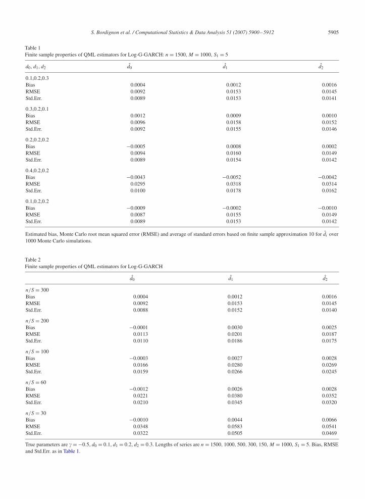
Table 1 lists the bias, Monte Carlo root mean squared error (RMSE) and average of the standard errors (Std.Err.),based on finite sample approximation (10), for d̂i across M = 1000 Monte Carlo simulations and for n = 1500. Fiveconfigurations of the parameter vector, each corresponding to different distributions of long-memory degrees amongfrequencies, were involved. Estimation results for are not shown but they are in line with those for the other parameters.Table 1 shows that all estimates are correctly centred at the true parameter values. The corresponding RMSE are verysmall and, as expected, tend to the values given by the standard errors.

Simulation results concerning the behaviour of our estimation procedure with respect to sample size n are listed inTable 2, in which S and the parameter vector are kept fixed (S = 5, = −0.5, d0 = 0.1, d1 = 0.2 and d2 = 0.3), whereas


Table 1Finite sample properties of QML estimators for Log-G-GARCH: n = 1500, M = 1000, S1 = 5

d0, d1, d2 d̂0 d̂1 d̂2

0.1,0.2,0.3Bias 0.0004 0.0012 0.0016RMSE 0.0092 0.0153 0.0145Std.Err. 0.0089 0.0153 0.0141

0.3,0.2,0.1Bias 0.0012 0.0009 0.0010RMSE 0.0096 0.0158 0.0152Std.Err. 0.0092 0.0155 0.0146

0.2,0.2,0.2Bias −0.0005 0.0008 0.0002RMSE 0.0094 0.0160 0.0149Std.Err. 0.0089 0.0154 0.0142

0.4,0.2,0.2Bias −0.0043 −0.0052 −0.0042RMSE 0.0295 0.0318 0.0314Std.Err. 0.0100 0.0178 0.0162

0.1,0.2,0.2Bias −0.0009 −0.0002 −0.0010RMSE 0.0087 0.0155 0.0149Std.Err. 0.0089 0.0153 0.0142

Estimated bias, Monte Carlo root mean squared error (RMSE) and average of standard errors based on finite sample approximation 10 for d̂i over1000 Monte Carlo simulations.

Table 2Finite sample properties of QML estimators for Log-G-GARCH

d̂0 d̂1 d̂2

n/S = 300Bias 0.0004 0.0012 0.0016RMSE 0.0092 0.0153 0.0145Std.Err. 0.0088 0.0152 0.0140

n/S = 200Bias −0.0001 0.0030 0.0025RMSE 0.0113 0.0201 0.0187Std.Err. 0.0110 0.0186 0.0175




True parameters are = −0.5, d0 = 0.1, d1 = 0.2, d2 = 0.3. Lengths of series are n = 1500, 1000, 500, 300, 150, M = 1000, S1 = 5. Bias, RMSEand Std.Err. as in Table 1.


Table 3Finite sample properties of QML estimators for Log-G-GARCH

d0, d1, d2, d3, d4—(S) d̂0 d̂1 d̂2 d̂3 d̂4

0.1,0.2—(3)

Bias −0.0012 −0.0004 — — —RMSE 0.0085 0.0142 — — —Std.Err. 0.0080 0.0136 — — —

0.1,0.2,0.2—(5)

Bias −0.0009 −0.0002 −0.0010 — —RMSE 0.0087 0.0155 0.0149 — —Std.Err. 0.0089 0.0153 0.0142 — —0.1,0.25,0.25,0.25—(7)

Bias −0.0006 −0.0164 0.001 0.0008 —RMSE 0.0102 0.025 0.0169 0.0149 —Std.Err. 0.0097 0.0161 0.0163 0.0146 —

0.1,0.25,0.25,0.25,0.25—(9)Bias 0.0000 0.0037 0.0027 0.0017 0.0027RMSE 0.0107 0.0166 0.0173 0.0175 0.0151Std.Err. 0.0105 0.0171 0.0169 0.0170 0.0152

n = 1500, M = 1000 and variable S, ratios n/S are 500, 300, 414 and 166 corresponding to S = 3, 5, 7, 9. Bias, RMSE and Std.Err. as in Table 1.

n, and thus the corresponding n/S ratio, changes. The chosen values for n are 150, 300, 500, 1000 and 1500. Table 2shows that the estimates of d0, d1 and d2 are satisfactory even for short time series and that Bias, RMSE and Std.Err.decrease consistently with increasing n.

Table 3 lists simulation results analysing the behaviour of the estimator with respect to a varying length of period S,but holding the sample size fixed at n = 1500. Its good performance is confirmed in this situation as well. In summary,our estimation procedure behaves quite well and seems rather robust with respect to changes of the n/S ratio.

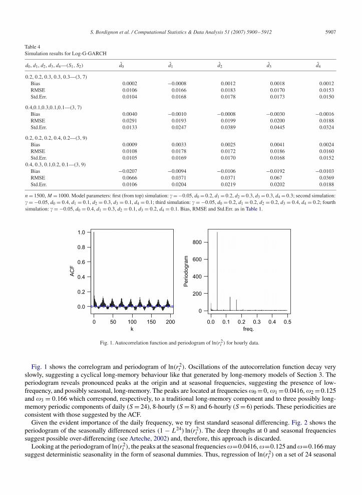
Now the special case in which the dynamics of the (log) conditional variance is driven by two periodic componentsis considered. Four particular situations, each characterised by differing lengths of the two periodic components, areexamined. In the first two S1 = 3 and S2 = 7, thus �1 = {0, 2�/3} and �2 = {0, 2�/7, 4�/7, 6�/7} and the onlyfrequency at which the two components overlap is �=0. The set of frequencies entailed by the Log-G-GARCH modelis � = {0, 2�/7, 4�/7, 2�/3, 6�/7} with h + 1 = 5. The long-memory parameters associated to the frequencies in �are, respectively, d0 =0.2, d1 =0.2, d2 =0.3, d3 =0.3, d4 =0.3 and d0 =0.4, d1 =0.1, d2 =0.3, d3 =0.1, d4 =0.1. Forthird and fourth simulations, two overlapping components are studied, setting S1 = 3 and S2 = 9. Thus �1 ={0, 2�/3},�2 ={0, 2�/9, 4�/9, 6�/9, 8�/9} and �={0, 2�/9, 4�/9, 2�/3, 8�/9}. Again, h+1=5. In this case the long-memoryparameters are d0 = 0.2, d1 = 0.2, d2 = 0.2, d3 = 0.4,d4 = 0.2 and d0 = 0.4, d1 = 0.3, d2 = 0.1, d3 = 0.2, d4 = 0.1.

Some simulation results are listed in Table 4. Once again, the effectiveness of our estimation procedure is confirmed.

6. Periodic long-memory patterns in the Euro–Dollar exchange rate

Since the pioneering works of Olsen and Associates (Gencay et al., 2001; Guillaume et al., 1997, 1995; Dacorognaet al., 1993; among others), foreign exchange market data have been examined for microstructural analysis purposes,to study the presence of heterogeneous agents and to test methodological improvements related to stylised facts suchas long-memory and periodic patterns in volatility. Following this line of the literature, an empirical application ofG-GARCH models to foreign exchange data is proposed, focusing on the Euro–Dollar exchange rate log-returns.

Data cover the period 1 January 2000–31 December 2004, and were provided by Olsen and Associates at a frequencyof 5-min, but in the application hourly data were considered. The length of the resulting series, omitting incompletedays, is n = 31 296.

The return time series is uncorrelated and thus no model for conditional mean is necessary. As usual, instead, thesquared residuals are correlated and show periodic behaviour. Since in the following we use log-GARCH-type models,hereafter we concentrate on log squared residuals, ln(r2

t ).


Table 4Simulation results for Log-G-GARCH

d0, d1, d2, d3, d4—(S1, S2) d̂0 d̂1 d̂2 d̂3 d̂4

0.2, 0.2, 0.3, 0.3, 0.3—(3, 7)

Bias 0.0002 −0.0008 0.0012 0.0018 0.0012RMSE 0.0106 0.0166 0.0183 0.0170 0.0153Std.Err. 0.0104 0.0168 0.0178 0.0173 0.0150

0.4,0.1,0.3,0.1,0.1—(3, 7)

Bias 0.0040 −0.0010 −0.0008 −0.0030 −0.0016RMSE 0.0291 0.0193 0.0199 0.0200 0.0188Std.Err. 0.0133 0.0247 0.0389 0.0445 0.0324

0.2, 0.2, 0.2, 0.4, 0.2—(3, 9)

Bias 0.0009 0.0033 0.0025 0.0041 0.0024RMSE 0.0108 0.0178 0.0172 0.0186 0.0160Std.Err. 0.0105 0.0169 0.0170 0.0168 0.0152

0.4, 0.3, 0.1,0.2, 0.1—(3, 9)

Bias −0.0207 −0.0094 −0.0106 −0.0192 −0.0103RMSE 0.0666 0.0371 0.0371 0.067 0.0369Std.Err. 0.0106 0.0204 0.0219 0.0202 0.0188

n = 1500, M = 1000. Model parameters: first (from top) simulation: = −0.05, d0 = 0.2, d1 = 0.2, d2 = 0.3, d3 = 0.3, d4 = 0.3; second simulation: = −0.05, d0 = 0.4, d1 = 0.1, d2 = 0.3, d3 = 0.1, d4 = 0.1; third simulation: = −0.05, d0 = 0.2, d1 = 0.2, d2 = 0.2, d3 = 0.4, d4 = 0.2; fourthsimulation: = −0.05, d0 = 0.4, d1 = 0.3, d2 = 0.1, d3 = 0.2, d4 = 0.1. Bias, RMSE and Std.Err. as in Table 1.

0 50 100 150 200

0.0

0.2

0.4

0.6

0.8

1.0

k

ACF

0.0 0.1 0.2 0.3 0.4 0.5

0

200

400

600

800

freq.

Periodogram

Fig. 1. Autocorrelation function and periodogram of ln(r2t ) for hourly data.

Fig. 1 shows the correlogram and periodogram of ln(r2t ). Oscillations of the autocorrelation function decay very

slowly, suggesting a cyclical long-memory behaviour like that generated by long-memory models of Section 3. Theperiodogram reveals pronounced peaks at the origin and at seasonal frequencies, suggesting the presence of low-frequency, and possibly seasonal, long-memory. The peaks are located at frequencies �0 =0, �1 =0.0416, �2 =0.125and �3 = 0.166 which correspond, respectively, to a traditional long-memory component and to three possibly long-memory periodic components of daily (S = 24), 8-hourly (S = 8) and 6-hourly (S = 6) periods. These periodicities areconsistent with those suggested by the ACF.

Given the evident importance of the daily frequency, we try first standard seasonal differencing. Fig. 2 shows theperiodogram of the seasonally differenced series (1 − L24) ln(r2

t ). The deep throughs at 0 and seasonal frequenciessuggest possible over-differencing (see Arteche, 2002) and, therefore, this approach is discarded.

Looking at the periodogram of ln(r2t ), the peaks at the seasonal frequencies �=0.0416, �=0.125 and �=0.166 may

suggest deterministic seasonality in the form of seasonal dummies. Thus, regression of ln(r2t ) on a set of 24 seasonal


0.0 0.1 0.2 0.3 0.4 0.5

0

5

10

15

20

freq.

Periodogram

Fig. 2. Periodogram of (1 − L24) ln(r2t ) for hourly data.

0.0 0.1 0.2 0.3 0.4 0.5

0

5

10

15

20

25

30

freq.

Periodogram

Fig. 3. Periodogram of deseasonalised ln(r2t ). The Y -axis is truncated at 30: actually the peak at zero frequency is about 100.

dummies was considered. The periodogram of deseasonalised ln(r2t ) (Fig. 3) shows that, even though seasonal dummies

removed the peaks at the specific frequencies relating to the daily and intra-daily cycles, there are still some peakslocated at neighbouring frequencies, which may indicate that the deterministic approach is not sufficient.

In order to explore in depth different approaches to data modelling, a FIGARCH model, including seasonal dummiesvariables in the conditional variance equation, was also tried. This kind of model, however, did not provide good results,as evidenced in the periodogram of the log-squared residuals (see Fig. 4).


0.0 0.1 0.2 0.3 0.4 0.5

0

200

400

600

800

freq.

Periodogram

Fig. 4. Periodogram of standardised squared residuals, ln(e2t ), of the FIGARCH model with seasonal dummies.

Table 5Log-G-GARCH model: estimated parameters for hourly data

Parameter d0 d1 d2 d3 d4

Estimate −0.09 0.301 0.399 0.261 0.315 0.319Std.Err. 0.009 0.007 0.033 0.020 0.024 0.020t-Stat. −9.280 44.786 12.022 13.148 13.154 16.143

Parameter d5 d6 d7 d8 d9 d10

Estimate 0.313 0.341 0.343 0.338 0.339 0.342Std.Err. 0.018 0.024 0.020 0.025 0.022 0.028t-Stat. 17.232 14.154 16.840 13.121 14.971 12.373

Parameter d11 d12 �1 �2 �24 1Estimate 0.341 0.154 −0.101 −0.08 0.690 −0.210Std.Err. 0.025 0.014 0.031 0.020 0.028 0.047t-Stat. 13.884 10.817 −3.180 −3.834 24.828 8.397

Parameter 2 3 4 24Estimate −0.152 −0.09 −0.06 0.371Std.Err. 0.031 0.022 0.017 0.034t-Stat. −4.868 4.091 −3.531 10.911

Since none of these methods gave satisfactory results, a Log-G-GARCH model was estimated for rt . The identifiedmodel is

ln(�2t ) = + �(L) ln(�2

t ) +⎧⎨⎩1 − �(L) −

⎡⎣(1 − L)d0(1 + L)d12

11∏j=1

(1 − 2 cos(�j )L + L2)dj

⎤⎦(L)

⎫⎬⎭ �̃2

t ,

where �̃2t = [ln(�2

t ) − ], �(L) = (�1L + �2L2 + �24L

24), (L) = (1 − 1L + 2L2 + 3L

3 + 4L4 + 24L

24) and�j = 2�j/24, (j = 1, . . . , 11).

Estimation results are shown in Table 5. Positivity restrictions on parameters are not needed because the logarithmof the conditional variance is modelled. Standard errors of parameters are computed by means of (10) and are givenwith the limitations described in Section 4.


0 50 100 150 200

0.8

0.6

0.4

0.2

0.0

1.0

k

ACF

0.0 0.1 0.2 0.3 0.4 0.5

0

5

10

15

20

25

30

freq.

Periodogram

Fig. 5. Autocorrelation function and periodogram of log-squared residuals of Log-G-GARCH model for hourly data.

0.0 0.1 0.2 0.3 0.4 0.5

0

50

100

150

200

freq.

Periodogram

0.0 0.1 0.2 0.3 0.4 0.5

0

500

1000

1500

freq.

Periodogram

Fig. 6. Periodograms of log-squared returns for 4-hourly (left) and half-hourly (right) data.

All the memory coefficients dj are significant and less than 0.5, in particular d0 = 0.301 and d1 = 0.399. Moreover,they are not very similar evidencing different degrees of long-memory at different frequencies. The correlogramof standardised log-squared residuals of the model is basically uncorrelated. The residual correlation shown by thecorrelogram is extremely weak (Fig. 5): the specific values of the estimated autocorrelations at the first seven lags are�̂1 =−0.016, �̂2 =−0.045, �̂3 =−0.034, �̂4 =−0.022, �̂5 =−0.051, �̂6 =−0.031 and �̂7 =−0.027. Therefore, for allpractical purposes, it can be neglected. Similarly, the periodogram of ln(e2

t ) does not show any dominant peak neitherat the seasonal frequencies nor at some neighbourhood (Fig. 5). Modelling volatility by G-GARCH models was thuseffective.

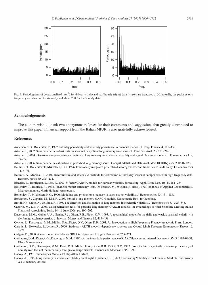
In the previous application, seasonality was treated as stochastic. It is interesting to note that this is not alwaysthe case and that the stochastic or deterministic nature of seasonality may be also connected with the frequency atwhich data are sampled. For example, Fig. 6 shows the periodograms of the Euro–Dollar exchange rate log-squaredreturns, for the same period, but sampled 4-hourly and half-hourly. In both cases, the peaks may suggest deterministicseasonality. However, the periodograms of deseasonalised ln(r2

t ), by regression on seasonal dummies, point out thatonly for the 4-hourly data the deterministic approach is effective, whereas for the half-hourly ones a stochastic modellingof seasonality seems more appropriate (Fig. 7).


0.0 0.1 0.2 0.3 0.4 0.5

0

5

10

15

20

25

30

freq.

Periodo

gram

0

5

10

15

20

25

30

Periodo

gram

0.0 0.1 0.2 0.3 0.4 0.5

freq.

Fig. 7. Periodograms of deseasonalised ln(r2t ) for 4-hourly (left) and half-hourly (right) data. Y -axes are truncated at 30: actually, the peaks at zero

frequency are about 40 for 4-hourly and about 200 for half-hourly data.

Acknowledgements

The authors wish to thank two anonymous referees for their comments and suggestions that greatly contributed toimprove this paper. Financial support from the Italian MIUR is also gratefully acknowledged.

References

Andersen, T.G., Bollerslev, T., 1997. Intraday periodicity and volatility persistence in financial markets. J. Emp. Finance 4, 115–158.Arteche, J., 2002. Semiparametric robust tests on seasonal or cyclical long memory time series. J. Time Ser. Anal. 23, 251–286.Arteche, J., 2004. Gaussian semiparametric estimation in long memory in stochastic volatility and signal plus noise models. J. Econometrics 119,

79–85.Arteche, J., 2006. Semiparametric estimation in perturbed long memory series. Comput. Statist. and Data Anal., doi: 10.1016/j.csda.2006.07.023.Baillie, R.T., Bollerslev, T., Mikkelsen, H.O., 1996. Fractionally integrated generalized autoregressive conditional heteroskedasticity. J. Econometrics

74, 3–30.Beltratti, A., Morana, C., 2001. Deterministic and stochastic methods for estimation of intra-day seasonal components with high frequency data.

Econom. Notes 30, 205–234.Bisaglia, L., Bordignon, S., Lisi, F., 2003. k-factor GARMA models for intraday volatility forecasting. Appl. Econ. Lett. 10 (4), 251–254.Bollerslev, T., Hodrick, R., 1992. Financial market efficiency tests. In: Pesaran, M., Wickins, R. (Eds.), The Handbook of Applied Econometrics I.

Macroeconomics, North-Holland, Amsterdam.Bollerslev, T., Mikkelsen, H.O., 1996. Modeling and pricing long memory in stock market volatility. J. Econometrics 73, 151–184.Bordignon, S., Caporin, M., Lisi, F., 2007. Periodic long-memory GARCH models. Econometric Rev., forthcoming.Breidt, F.J., Crato, N., de Lima, P., 1998. The detection and estimation of long memory in stochastic volatility. J. Econometrics 83, 325–348.Caporin, M., Lisi, F., 2006. Misspecification tests for periodic long memory GARCH models. In: Proceedings of 43rd Scientific Meeting Italian

Statistical Association, Turin, 14–16 June 2006, pp. 199–202.Dacorogna, M.M., Müller, U.A., Nagler, R.J., Olsen, R.B., Pictet, O.V., 1993. A geographical model for the daily and weekly seasonal volatility in

the foreign exchange market. J. Internat. Money and Finance 12, 413–438.Gencay, R., Dacorogna, M.M., Müller, U.A., Pictet, O.V., Olsen, R.B., 2001. An Introduction to High Frequency Finance. Academic Press, London.Giraitis, L., Kokoszka, P., Leipus, R., 2000. Stationary ARCH models: dependence structure and Central Limit Theorem. Econometric Theory 16,

3–22.Guégan, D., 2000. A new model: the k-factor GIGARCH process. J. Signal Process. 4, 265–271.Guillaume, D.M., Pictet, O.V., Dacorogna, M.M., 1995. On the intra-daily performance of GARCH processes. Internal Document DMG. 1994-07-31,

Olsen & Associates.Guillaume, D.M., Dacorogna, M.M., Davé, R.D., Müller, U.A., Olsen, R.B., Pictet, O.V., 1997. From the bird’s eye to the microscope: a survey of

new stylized facts of the intra-daily foreign exchange markets. Finance and Stochast 1, 95–129.Harvey, A., 1981. Time Series Models. Phillip Allan, Oxford.Harvey, A., 1998. Long memory in stochastic volatility. In: Knight, J., Satchell, S. (Eds.), Forecasting Volatility in the Financial Markets. Butterworth

& Heinemann, Oxford.


Hylleberg, S., 1986. Seasonality in Regression. Academic Press, Oxford.Kazakeviéius, V., Leipus, R., 2002. On stationarity in the ARCH(∞) model. Econometric Theory 18, 1–16.Reisen, V.A., Rodrigues, A.L., Palma, W., 2006. Estimation of seasonal fractionally integrated processes. Comput. Statist. Data Anal. 50, 568–582.Woodward, W.A., Cheng, Q.C., Gray, H., 1998. A k-factor GARMA long-memory model. J. Time Ser. Anal. 19 (4), 485–504.Zaffaroni, P., 2004. Stationarity and memory in ARCH(∞) models. Econometric Theory 20, 147–160.

generalised long-memory garch models for intra-daily volatility

Documents