(general issues, interpretation of results, potential

Numerical Computing - before you start

(General issues, Interpretation of results, potential troubles and traps, etc. ..)

(... strong emphasis on accelerators)

Werner Herr, Numerical computing, Thessaloniki, 12.11.2018

Some (maybe less known) Reading Material

[LL ] A.Lichtenberg and M.Lieberman, Regular and Chaotic Dynamics,

Applied Mathematical Sciences 38, Springer, New York, 1983.

[SC ] J.B. Scarborough, Numerical Mathematical Analysis, Oxford University

Press, Oxford, 1958.

[TF ] T. Ferris, Coming o f age in the Milky Way, HarperCollins, New York,

2003.

[EA ] D. Earn et.al. Physica D 56 (1992).

[RN ] P. Rannou, Astron. Astrophys. 31, 289.

The purpose of computing for science is insight, not numbers

Dealing with Dynamic Systems it is usually difficult and most likely impossible to

find analytical solutions (at least the interestings ones).

The most reliable tools to study Realistic models, e.g. an accelerator, are numerical

methods (e.g. amongst others: numerical evaluation of Differential Equations and

tracking codes)

Understanding the quality of a numerical method is the key to understand the

behaviour of e.g. an accelerators.

This lecture is not at all meant as an thorough computer science discussion,

( i.e. it is liberated from the shackle of a syllabus) rather to cover topics for no

more reason that they are interesting and useful

just writing some code is not enough (by far !)

Numerical methods have limitations !!

The purpose of computing for engineering are numbers, not insight

Dealing with Dynamic Systems it is usually difficult and most likely impossible to

find analytical solutions (at least the interestings ones).

The most reliable tools to study Realistic models, e.g. an accelerator, are numerical

methods (e.g. amongst others: numerical evaluation of Differential Equations and

tracking codes)

Understanding the quality of a numerical method is the key to understand the

behaviour of e.g. an accelerators.

This lecture is not at all meant as an thorough computer science discussion,

( i.e. it is liberated from the shackle of a syllabus) rather to cover topics for no

more reason that they are interesting and useful

just writing some code is not enough (by far !)

Numerical methods have limitations !!

Therefore: "A man’s got do know his limitations" (courtesy Dirty Harry)

If you write complex scientific computer codes and do not take into account the

limitations (yours, the computer’s and other issues), you will flop !

Therefore: "A good man always knows his and his computer′s limitations︸︷︷︸

this we discuss

"

Discuss and analyse some limitations - Menu

��

��

Numerical Analysis (can we rely on numbers ?)

��

��

Model versus algorithm (do we have a preference ?)

��

��

Chaos, (artifical or true ?) and all that ..

��

��

Lattice Map (a rescue for some problems ?)

��

��

...

Will touch on a few concepts treated in detail in following lectures, may/should

provide some awareness (unlike sometimes said: we shall do more than discussing

LINUX versus WINDOWS)

Numerical analysis - (some) typical issues:

��

��

Intrinsic errors using computers (not programmer’s faults)

��

��

Inappropriate algorithms

��

��

Roundoff errors

��

��

Truncation errors

��

��

Conversion errors

Be aware of potential numerical and conceptual difficulties that may exist.

��

��

Numbers are part or the problem, not the answer

Most (if not all) of the following may sound familiar , but the consequences strongly

affect the computation and the analysis of the results ! Be prepared and avoid

being dogmatic ...

Here is a purpose - challenges for LHC experiments:

Need to understand what the

computer is doing ..

- More than 40 collisions

- Numerically challenging

- Requires careful analysis

Spot the "Higgs"

- Wrong conclusion would be

very embarrasing

- Wrong statements are em-

barrasing

Wrong numbers wrong conclusions wrong statements no price

Numbers (Computers versus mathematicians versus physicists):

Integer, fixed point and floating point (complex ignored for the time being):

��

��

Integers: usually do not pose any problem:

- Unique represention

- Finite range (due to word length) Note: starts with 0

��

��

Fixed point numbers: e.g. 2.71828, 3.14159265∗, 299792458.000:

- Fixed length (usually linked to word length), machine always keeps the

same number of digits, limited range

- An important use: banking ! (you do not want 16.049999993 · 103 CHF)

- Fast and easier to implement in hardware (but see later ...)

Floating point numbers:

Internal representation of floating point numbers use a fixed number of binary

digits to represent a decimal number. Some (most) decimal numbers cannot

be represented exactly in binary, resulting in problems already for basic

operations (addition, subtraction, multiplication, division)

∗ troubles ahead ..

��

��

Floating point numbers, some issues:

- So-called scientific notation, e.g. 0.000271828 × 104:

- In mathematics, there is a single 0

But: 0, − 0 , .000 × 10−9, .000 × 10+9

are logically the same, but some machines or programming languages

make them the same, others do not ! (sometimes for good reasons)

- Related: 1.00 · 10−1 and 0.01 · 101 are stored differently

This has some very unpleasant consequence !

��

��

Finite arithmetic in mathematics not the same as finite arithmetic of machines

��

��

Floating point numbers are a trade-off between range and precision

This can/will have strong implications for writing scientific software

First troubles - Floating point Representation on different machines

CERN in the late ’70: mainly 3 types of mainframes; CDC, IBM, VAX

Double precision floating point (64 and 60 bits) representation was:

VAX

CDCsign bit

exponent

( it is true !)

IBM

mantissa

2nd 1st

3rd4th

Exchange of binary floating point numbers somewhat difficult ...

Common standard as defined by IEEE 754 (1985)

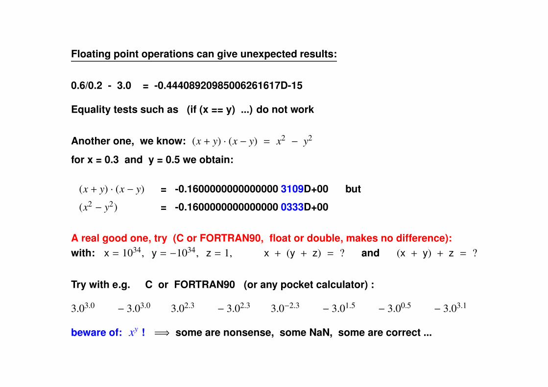
Floating point operations can give unexpected results:

0.6/0.2 - 3.0 = -0.44408920985006261617D-15

Equality tests such as (if (x == y) ...) do not work

Another one, we know: (x + y) · (x − y) = x2 − y2

for x = 0.3 and y = 0.5 we obtain:

(x + y) · (x − y) = -0.1600000000000000 3109D+00 but

(x2 − y2) = -0.1600000000000000 0333D+00

A real good one, try (C or FORTRAN90, float or double, makes no difference):

with: x = 1034, y = −1034, z = 1, x + (y + z) = ? and (x + y) + z = ?

Try with e.g. C or FORTRAN90 (or any pocket calculator) :

3.03.0 − 3.03.0 3.02.3 − 3.02.3 3.0−2.3 − 3.01.5 − 3.00.5 − 3.03.1

beware of: xy ! =⇒ some are nonsense, some NaN, some are correct ...

Consider the function:

f (x) =1

x − 1

x f(x)

1.100000 9.9999976

1.001000 999.9532721

1.000100 9998.3408820

1.000010 99864.380952

1.000001 1048576.000000

10.100000 0.109890

10.001000 0.111099

10.000100 0.1111098

10.000010 0.1111109

10.000001 0.1111110

l|l

well behaved for small changes near x = 10

ill-conditioned for small changes near x = 1 (check and avoid)

Iterative systems - circular accelerators:

The use of computers and numerical methods may require a large number of

iterations - typical example simulations for a (circular) machine

��

��

Iterative systems usually means that results from one stage of the

computation are used in subsequent calculations, i.e. a feedback situation

��

��

Small errors are propagated and can lead to:

- Loss of precision of the results

- Artifacts leading to wrong conclusions and wrong physics

��

��

A powerful tool for (accelerator) simulations but can lead to problems:

Examples mainly for beam dynamics, but problems can be the same everywhere

(some examples later ..)

At every iteration only a fixed number of digits is retained, rounded nearby the

representable number. The problems:

- The "Hamiltonian properties" (see later) are not preserved, can become

dissipative hence in the worst case violate Liouville’s theorem (see later):

worst case scenario ..

- For a small number of iterations it is probably not dramatic

- The cumulative effect can/will lead to significant changes to the long-term

behaviour of e.g. trajectories =⇒ can lead to completely wrong conclusions ..

The standard argument: use Double Precision and we are save.

Is this always true for practical applications ?

An iterative process IEEE 80 (!) bit precision (both formulae are equivalent):

p0 =1√3

and q0 =1√3

pi+1 =

√

p2i + 1 − 1

pi

and qi+1 =qi

√

qi2 + 1 + 1

with : 6 · 2i · pi with : 6 · 2i · qi

0.315965994209750084D+01 0.315965994209750084D+01 Starting point

0.314271459964536861D+01 0.314271459964536865D+01 Iteration 1

0.314166274705685013D+01 0.314166274705684888D+01 ...

0.314159703432150639D+01 0.314159703432152650D+01

0.314159292738506092D+01 0.314159292738509738D+01

0.314159267069799892D+01 0.314159267070199840D+01

0.314159265460636674D+01 0.314159265465930638D+01

0.314159265260533476D+01 0.314159265365663814D+01

0.314159264193316416D+01 0.314159265359005470D+01

0.314159264193316416D+01 0.314159265358979461D+01

0.304383829792641763D+01 0.314159265358979359D+01

0.295679307476062510D+01 0.314159265358979359D+01

NaN 0.314159265358979359D+01

Size matters:

Normally 64-bit floating point arithmetic is fully sufficient.

But for numerically sensitive calculations it may be questionable∗. May in turn

induce other errors: e.g. wrong decision in a conditional branch or real

pathological results.

Some examples where higher precision is needed:

- Supernova simulations (non-local thermodynamic equilibrium)

- Climate modelling

- Planetary orbit calculation [TF], black hole merger (astrophysicists are

smart(er) !)

- LHC experiments: Quark, Gluon and Vector Boson scattering. If a phase space

point is numerically unstable: recomputed with higher precision

- Large matrices (e.g. n × n with n as large as 107) with large condition numbers

∗ most likely insufficient !

Most programming languages can use arbitrary precision floating point arithmetic using (free)

libraries e.g.: popular one for Python is MPMAT H. Also ARPREC for FORTRAN 90 and C++.

UNIX based (also MAC OSX): MPFUN2015 for FORTRAN 90 which requires very little changes

to existing programs (mainly types).

Some issues:

Have to take into account when the code is written: may/does require individual calls to

library routines for each arithmetic calculation. Much easier with MPFUN2015.

Slow execution time, e.g. rule of thumb compared to 64 bits (17 digits):

- 31 digits: × 5

- 62 digits: × 25

- 100 digits: × 50

- 1000 digits: × 1000

Rather hard to debug

Can cause user fatigue and most scientists give up ... (except maybe a few)

Better if sufficiently high precision is inbuilt !

Behind your back - Consider the programs:

int main1()

{

double x, y;

x = 4.0/9.0;

y = 8.0/18.0;

if (x == y)

printf("nice");

else

printf("not nice");

}

int main2()

{

double x, y;

x = 4.0/9.0;

y = 8.0/18.0;

if (x == 8.0/18.0)

printf("nice");

else

printf("not nice");

}

The results ??

Behind your back - Consider the programs:

int main1()

{

double x, y;

x = 4.0/9.0;

y = 8.0/18.0;

if (x == y)

printf("nice");

else

printf("not nice");

}

int main2()

{

double x, y;

x = 4.0/9.0;

y = 8.0/18.0;

if (x == 8.0/18.0)

printf("nice");

else

printf("not nice");

}

The results:

- main1: will always give you nice !

- main2: nice or not nice, Hardware and/or Compiler dependent !

Lesson 1: use a smart compiler with very smart optimizer !

Lesson 2: use it like in main1()

Included datatypes. Furthermore, popular languages, i.e. C++ and FORTRAN 95 and PYTHON

allow operator overloading (practical example in the coming few days), this makes it less

painful. Examples:

FORTRAN (95 or higher)

- Proper Quad Precision (128 bits, up to 62 digits) with e.g.:

My128 = selected_real_kind(32), My128 is then the TYPE

- "Quad" Precision (80 bits, up to 62 digits) with e.g.:

My80 = selected_real_kind(10), My80 is then the TYPE

For some compilers you can write: REAL*10 and REAL*16 (don’t !)

C/C++

- VERY compiler and hardware dependent (there is no IEEE standard):

long double can be anything between 64 and 80 bit precision,

80 bit is often proper 128 with padding for alignment

Proper 128 bit with _Quad on Intel compiler

NO support on Microsoft VC, everything converted to standard double

Very different for Mathematica, Matlab, etc. ...

Examples, using 1/10 different languages and types (inbuilt, incomplete):

FORTRAN and C++ single precision:

0.10000000149011612 i.e. 6 - 7 reliable significant digits

FORTRAN and C++ double precision:


PYTHON double precision (printed using DECIMAL):


FORTRAN using selected_real_kind(p=18) i.e. 18 significant digits

0.10000000000000000001

Available on some (UNIX !) machines and compilers (e.g. DIGITAL FORTRAN 90)

selected_real_kind(p=33) i.e. 33 significant digits

Mixing different precisions or types: you should know exactly what you are doing !

(e.g. byte streams in communication, TCP)

Use typecasting wherever possible .. (rather good in C++)

Integers have "higher" precision that single floats !!! :

try:

#include <stdio.h>

int main(void)

{

int myint = 16777217;

float myfloat = 16777216.0;

printf("my integer is: %d", myint);

printf("my float is: %f", myfloat);

printf("equality ? %d", myfloat == myint);

}

Result ?

Integers have "higher" precision that single floats !!! :

try:

#include <stdio.h>

int main(void)

{

int myint = 16777217;

float myfloat = 16777216.0;

printf("my integer is: %d", myint);

printf("my float is: %f", myfloat);

printf("equality ? %d", myfloat == myint);

}

Result:

my integer is: 16777217

my float is: 16777216.000000

equal ?: 1 (means they are found to be equal)

integer can store 224, floating point mantissa is too small (23)

Most problematic: rounding and truncation

Rounding of constants to integers following the IEEE 754 standards:

Mode/Example 5.5 6.5 -5.5 -6.5

to nearest, tied to even 6.0 6.0 -6.0 -6.0

to nearest, tied away from 0 6.0 7.0 -6.0 -7.0

toward 0 (truncation !) 5.0 6.0 -5.0 -6.0

toward +∞ (ceiling) 6.0 7.0 -5.0 -6.0

toward −∞ (floor) 5.0 6.0 -6.0 -7.0

some examples to remember:

1 f loat to int causes truncation, i.e., removal of the fractional part.

2 double to f loat causes rounding of digit.

3 long to int causes dropping of excess higher order bits.

After floating point operation:

(63.0/9.) to integer gives: 7

(0.63/0.09) to integer gives: 6

machine dependent !!!

However: Integer to floating point is mostly (!) well behaved

Some computer languages allow to control the truncation/roundoff, e.g. float to

integer (C++, FORTRAN 90, Python, ...):

a) Integer part of x (x is truncated)

b) Nearest integer to x (x is rounded)

Some more (no guarantee that it is always true):

Python 3.0 gives: 5/2 = 2.5, 5//2 = 2, 5.0//2 = 2.0

99/3 is float, 99//3 is integer (// means f loor)

FORTRAN 95: 9999999999999999/3 = 3333333333333333

keeps integer (if the result is integer)

Fore some fun: 0.1 is never correctly represented

e.g. with high precision:

0.1 = 0.1000000000000000055511151231257827021181583404541015625

(unlikely to be relevant)

single precision: 0.1 = 0.10000000149011612

Conditional branches make a very big difference whether defined as floating point

or fixed point: different use of significant digits !

- Trouble with small numbers ...

subtraction of almost equal numbers may cause extreme loss of accuracy

the most significant digits become 0

- Typical example - computing derivatives:

the derivatives are computed as :f (a + h) − f (a)

h

For smaller h also f (a + h) − f (a) becomes smaller and makes the least

significant digits more important

Side note: programming languages such as C, C++, FORTRAN2003 support

infinities - they just follow some rules

a) +∞ + 5 = +∞

b) +∞ × − 5 = −∞

c) +∞ × 0 = NaN (not meaningful)

Why ? they can be used in conditional branches

f(x) = x2+

1

x+ 14x

f(x) = x2.5

10

12

14

16

18

20

22

0 2e-05 4e-05 6e-05 8e-05 0.0001

Der

ivat

ives

h

h dependence in derivative

the derivatives are computed as :f (a + h) − f (a)

h

For small h the calculation of the derivatives becomes unstable/useless

Lesson: avoid subtraction of close numbers !

If you want to do better: wait ..

In this context: A (true !) everyday example - LHC input for a popular optics program:

From database:

s.ds.r1.b1:omk, at= 268.904

mco.8r1.b1:mco, at= 269.248

mcd.8r1.b1:mcd, at= 269.2495

mb.a8r1.b1:mb, at= 276.734

mcs.a8r1.b1:mcs, at= 284.158

mb.b8r1.b1:mb, at= 292.394

mcs.b8r1.b1:mcs, at= 299.818

bpm.8r1.b1:bpm, at= 300.697

mqml.8r1.b1:mqml, at= 303.842

mcbcv.8r1.b1:mcbcv, at= 306.884

mco.9r1.b1:mco, at= 308.313

mcd.9r1.b1:mcd, at= 308.3145

mb.a9r1.b1:mb, at= 315.799

mcs.a9r1.b1:mcs, at= 323.223

mb.b9r1.b1:mb, at= 331.459

mcs.b9r1.b1:mcs, at= 338.883

bpm.9r1.b1:bpm, at= 339.763

mqmc.9r1.b1:mqmc, at= 341.739

mqm.9r1.b1:mqm, at= 345.005

mcbch.9r1.b1:mcbch, at= 347.346

... after "slicing" (sometimes needed, see this afternoon and tomorrow):

s.ds.r1.b1: omk, at = 268.903999999999996

mco.8r1.b1: mco, at = 269.247999999999990

mcd.8r1.b1: mcd, at = 269.249500000000012

mb.a8r1.b1, at = 276.734247349421594

mcs.a8r1.b1, at = 284.158494698843185

mb.b8r1.b1, at = 292.394742048264789

mcs.b8r1.b1, at = 299.818989397686323

bpm.8r1.b1: bpm, at = 300.697989397686342

mqml.8r1.b1..1, at = ( 303.84298939769 ) + ( ( l.mqml ) * ( 0 - 0.33333333333333 ) )

mqml.8r1.b1, at = 303.842989397686324 e.g. its strength: kq8 = -0.00694900907253902

mqml.8r1.b1..2, at = ( 303.84298939769 ) + ( ( l.mqml ) * ( 0.33333333333333 ) )

mcbcv.8r1.b1, at = 306.884989397686354

mco.9r1.b1: mco, at = 308.313989397686328

mcd.9r1.b1: mcd, at = 308.315489397686349

mb.a9r1.b1, at = 315.800236747107931

mcs.a9r1.b1, at = 323.224484096529523

mb.b9r1.b1, at = 331.460731445951126

mcs.b9r1.b1, at = 338.884978795372717

bpm.9r1.b1: bpm, at = 339.764978795372713

comments ??

... after "slicing" (sometimes needed, see this afternoon and tomorrow):

s.ds.r1.b1: omk, at = 268.903999999999996

mco.8r1.b1: mco, at = 269.247999999999990

mcd.8r1.b1: mcd, at = 269.249500000000012

mb.a8r1.b1, at = 276.734247349421594

mcs.a8r1.b1, at = 284.158494698843185

mb.b8r1.b1, at = 292.394742048264789

mcs.b8r1.b1, at = 299.818989397686323

bpm.8r1.b1: bpm, at = 300.697989397686342

mqml.8r1.b1..1, at = ( 303.84298939769 ) + ( ( l.mqml ) * ( 0 - 0.33333333333333 ) )

mqml.8r1.b1, at = 303.842989397686324 e.g. its strength: kq8 = -0.00694900907253902

mqml.8r1.b1..2, at = ( 303.84298939769 ) + ( ( l.mqml ) * ( 0.33333333333333 ) )

mcbcv.8r1.b1, at = 306.884989397686354

mco.9r1.b1: mco, at = 308.313989397686328

mcd.9r1.b1: mcd, at = 308.315489397686349

mb.a9r1.b1, at = 315.800236747107931

mcs.a9r1.b1, at = 323.224484096529523

mb.b9r1.b1, at = 331.460731445951126

mcs.b9r1.b1, at = 338.884978795372717

bpm.9r1.b1: bpm, at = 339.764978795372713

303.842989397686324 is NOT a useful number, in the worst case may lead to problems

It is not just academic (non scientific incidents):

- 1991: Truncation after multiplication of an integer (time) with 0.1 to convert to

a floating point number prevented a MIM-Patriot from intercepting a SCUD

proposed bug fix: always reboot after 8 hours of operation

- 1996: ARIANE 5 off trajectory and self-destructed: converted 64 bit float to 16

bit unsigned integer (too large)

- 1992: Wrong initial report of result from German election (4.97 % rounded to

5.0 %)

- 1982: Vancouver stock exchange: index from 1000.00 to 520.00 in 2 month

(should have been 1100, after each transaction the value was not rounded but

truncated)

- 2025:

Discussion 1:

- Be aware of (unavoidable) numerical problems

- Avoid being dogmatic: problems are intrinsic, the choice of your favorite

operating system or programming language does not help at all (the issues

may even be different and re-writing can become tricky) : it is not the ink that

makes the splotches

This means that programmers need to implement their own method of detect-

ing when they are approaching an inaccuracy threshold, must guard against it

at all times !

Or else give in the quest for a robust, stable implementation of an algorithms.

Some algorithms can be scaled so that computations don’t take place in the

constricted area near problems. However, scaling the algorithm and detecting the

inaccuracy threshold can be difficult and time-consuming for each numerical

problem.

Next: implications for interpretation of beam dynamics calculations

Terms important for dynamics (stability) of particles - stochastic versus chaotic

behaviour

Confusion alert they may appear equivalent from the point of view of an

observer, but are totally different phenomena:

- Stochastic motion is random at all times and all amplitudes

- Chaotic motion is predictable in the short term, but can appear random at

longer time and periods of an iterative system. At long term because it is very

sensitive to initial conditions and intrinsic to the dynamics, usually depends

on particle amplitudes (dynamic aperture)

To determine a "dynamic aperture" (see other lectures) stochastic contributions

should be avoided and are often due to one of these problems:

- Random by construction (e.g. "Monte Carlo" simulations)

- Random due to external noise (e.g. power converters, vibrations, ...)

- Numerical noise, in particular truncation or rounding

"Chaotic behaviour" is what we may want to study/observe

Some of our main interests:

��

��

Is the machine stable ?

��

��

Do we observe chaos (of the motion) ?

If we do "observe" chaotic motion:

��

��

Chaotic motion should be intrinsic to the dynamics and not the result of

numerical artifacts associated with finite precision arithmetic

��

��

Can easily be due to a not absolutely exact method of integration

Key: need an unambiguous understanding of a physical mechanism and whether

this mechanism really accounts for the observed chaos

The underlying model (e.g. the description of the machine, no need for attometer

precision) can be an approximation (which is always the case !), the algorithm must

be exact (within the limitations of the computer itself, i.e. truncation errors etc.).

Some keywords here, the gory details in other lectures: Hamiltonians,

symplecticity, Lie integrators, lattice maps, ...

Anticipating a following lecture, a key issue for the stability of a simulation (in

particular iterations) is the concept of symplecticity (will come many times).

Symplecticity in a nutshell (consider a pendulum):

Equation of motion (2D):

q̈(t) = − g

L· sin(q(t))

Reduce to 2 equations 1D:

q̇(t) = v(t)

v̇(t) = − g

L· sin(q(t))

L

q(t)

1. Break time t into steps ∆t: → tk = k · ∆t "time" is now a discrete variable tk

2. q(t) → qk and v(t) → vk

3. Solve for qk+1 and vk+1 (various methods)

Method 1 (fast, unstable, bad accuracy, energy blows up):

qk+1 = qk + ∆t · vk

vk+1 = vk − ∆t · g

L· sin(qk)

Method 2 (stable, slow, bad accuracy, energy dissipative):

qk+1 = qk + ∆t · vk+1

vk+1 = vk − ∆t · g

L· sin(qk+1)

Method 3 (stable, good accuracy, energy conserved, symplectic):

qk+1 = qk + ∆t · vk+1

vk+1 = vk − ∆t · g

L· sin(qk)

The third is the best known (Hamiltonian) map and is called the "standard

map"

Dealing with the standard map (plotted in Phase Space - x versus px:

K = 0.50 K = 0.97 K = 2.00

The behaviour, e.g. regular or chaotic motion depends on the parameter K =g

L

Transition to chaotic/stochastic layers appear for K = 0.97

However, for studying very long term behaviour: due to roundoff or truncation

errors, the standard map will always produce some chaos.

How to detect chaotic behaviour ?

A standard procedure: evaluate Lyapunov exponent, e.g. [LL]

"It characterizes the rate of separation of initially infinitesimally close (!)

trajectories"

a measure for the stability of a dynamic system, therefore a critical parameter

to be evaluated

It cannot be computed analytically, hence must rely on numerical techniques.

Typical use in accelerator design: single particle tracking to estimate region of

stability of trajectories (dynamic aperture). In the long term particles can "slip" into

chaotic region.

Track two particles initially very close in Phase Space and see what happens ...

LHC with two beam-beam interactions

Two particles started very close in Phase

Space

Plotted:

Phase Space distance after tracking 105 iter-

ations (turns, corresponds to ≈ 109 machine

elements in this case)0.0001

0.001

0.01

0.1

1

2 3 4 5 6 7 8 9 10

Dis

tan

ce

in

Ph

ase

Sp

ace

of

2 in

itia

lly c

lose

−b

y P

art

icle

s

Initial Amplitude [sigma]

HH crossing, 100000 turns, no errors, nominal bunches

Phase Space distance between the particles "jumps" by 2 orders of magnitude (and

stays up)

Depends only on particle amplitudes (in this example ≈ 6 σ) clear evidence for

onset of chaotic behaviour - in this case cross-checked with another parameter

The physics:

nonlinear beam-beam interactions make particles unstable at large amplitudes

Another example:

Again: LHC with two beam-beam interactions

(but different parameters)

An unstable "band" followed by a "stable re-

gion"0.0001

0.001

0.01

0.1

1

2 3 4 5 6 7 8 9 10

Dis

tan

ce

in

Ph

ase

Sp

ace

of

2 in

itia

lly c

lose

−b

y P

art

icle

s

Initial Amplitude [sigma]

HH crossing, PACMAN bunches

The corresponding Phase Space structures can be reproduced (maybe in another

lecture)

Depends only on particle amplitudes (in this example ≈ 6 σ) clear evidence for

onset of chaotic behaviour - in this case cross-checked with another parameter

The physics:

nonlinear beam-beam interactions make particles unstable at large amplitudes, but

hit a resonance at smaller amplitudes, then stable again

Not just accelerators - largest chaotic system: Solar System

Pluto: orbit highly inclined and eccen-

tric (crosses the Neptune orbit !)

Motion chaotic (but not unstable) due

to resonance with Neptune

Maybe also exhibit "stable bands" !

(beyond Saturne)

Requires N-body simulation (long

term, over Myrs or Gyrs)

Problems very similar to beam stability: chaos, roundoff, symplecticity, etc. Can we

profit from those studies ?

"Exact Numerical Studies of Hamiltonian Maps, Iterating without roundoff Errors",

D. Earn et.al. Physica D 56 (1992)

last part of this lecture ...

How does this relate to a (circular) accelerator ?

Take the most trivial example: Linear Motion in 1D (remember High School)

Consider one turn as a time step for this exercise (in reality the machine is

split into many time steps around the whole machine, but the arguments don’t

change)

Plotting the variables (now x and px) once per turn (again see later lecture) one gets

an ellipse in phase space:

-0.0004

-0.0003

-0.0002

-0.0001

0

0.0001

0.0002

0.0003

0.0004

-2 -1.5 -1 -0.5 0 0.5 1 1.5 2

px

x

Exact quadrupole versus thin lens approximation

Exact map

The exact model of the machine and exact algorithm are used

A non-symplectic solution

-0.0004

-0.0003

-0.0002

-0.0001

0

0.0001

0.0002

0.0003

0.0004

-2 -1.5 -1 -0.5 0 0.5 1 1.5 2

px

x


An exact and a non-symplectic map

Non-symplecticity: particles spiral towards outside (could also go to the

inside), artifact of the algorithm

exact model, but approximated algorithm

drawing conclusions from that is totally careless (but frequently happens)

the lesson: make sure the physical mechanism can be explained

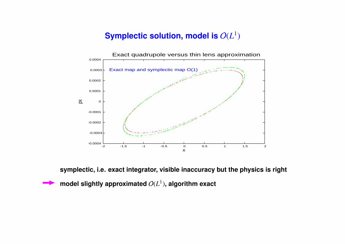
Symplectic solution, model is O(L1)

-0.0004

-0.0003

-0.0002

-0.0001

0

0.0001

0.0002

0.0003

0.0004

-2 -1.5 -1 -0.5 0 0.5 1 1.5 2

px

x


Exact map and symplectic map O(1)

symplectic, i.e. exact integrator, visible inaccuracy but the physics is right

model slightly approximated O(L1), algorithm exact

Symplectic solution, improved model ( O(L2))

-0.0004

-0.0003

-0.0002

-0.0001

0

0.0001

0.0002

0.0003

0.0004

-2 -1.5 -1 -0.5 0 0.5 1 1.5 2

px

x


Exact map and symplectic map O(2)

symplectic (in theory ), solution with model order O(L2), but already

good accuracy

Lesson from that→ different cases:

Model approximate and algorithm approximate

Model exact and algorithm approximate

Model approximate and algorithm exact

Model and algorithm exact

Only the two latter are acceptable, otherwise the physics stinks

There is no general remedy to improve approximate models but errors due

to approximate algorithms should be made as small as possible.

Back to the standard map:

Is it possible to avoid truncation and roundoff errors ?

For very long term tracking (e.g. Gyrs) eventually one is beaten by truncation and

roundoff errors - all machines are finite ..

Are there any numbers not (or less) troubled by these (unavoidable) errors?

��

��

For Fixed Point numbers bits are eliminated, but some rounding is done before

the elimination. Better than just truncation.

All integer numbers: They are limited by the number of bits, but no truncation

or roundoff. No chaos or stochastic behaviour can come from numerical

artifacts.

But can Integer Numbers be used for anything useful ?

Prerequisites: integration technique, method 3

It is usually used to integrate trajectories for a Hamiltonian like: H =1

2v2+ U(x, t)

x(t + ∆t) = x(t) + ∆t · x′(t + ∆t)

x′(t + ∆t) = x′(t) + A · ∆t · x(t)

A is the force derived from the potential: A = − ∇U(x, t)

To "cure" the truncation errors: multiply the potential by a (periodic) time

dependent factor with average zero:

H̃ =1

2v2+ U(x, t) ·

∑

n

δ(t − n · ∆t)

First→ introducing Lattice Maps:

Usually one uses floating point maps:

xn+1 = xn + something

yn+1 = yn + something

The time dependence of x and y is continuous.

Lattice maps:

- Each element is set on a lattice with given dimension

- Map: time is discrete

- Lattice: space is discrete

Solving Differential equations often using this procedure

Replace time step by finite, discrete steps

xn+1 = xn + ∆t · x′n+1︸︷︷︸

dri f t

x′n+1 = x′n + A · ∆t · xn︸︷︷︸

kick

It can be considered as a sort of "kick" and a "drift" and A is the force derived from

the potential: A = − ∇U(x, t)

Now going for the roundoff error Integer Lattice maps [EA, RN]

After change of scale, lattice points have integer coordinates, iterations are done

without error

The scheme is now: the function Ψ itself is discretized onto a lattice with:

Integer Grid Points (m, n) lattice points have Integer Coordinates !.

Integer coordinates do the iterations on the nodes without rounding errors.

The nodes are separated by ∆x and ∆x′. Each node has a value Ψ(m, n) of the

distribution function.

Important: for a lattice with m points per unit, the time step ∆t must be choosen so

that m · ∆t becomes an integer.

The procedure "shifts" particles on the lattice (from one lattice point to another).

With each time step ∆t the value Ψ(m, n) is updated to a new lattice node using a

"kick" and "drift" step, i.e.

n + [∆t · A] → n followed by m + [∆t · n] → m

Each node represents a point in Phase Space (not necessarily a single particle)

m∆

n∆

m

n

n∆

m∆

m

n

With each time step ∆t the value Ψ(m, n) is updated to a new lattice node using a

"drift" and "kick" step, i.e.

n + ⌊∆t · A⌉ → n ”kick”, left picture

m + ⌊∆t · n⌉ → m ”drift”, right picture

Xn, Yn are integers. Note: ⌊...⌉ is the operator: "rounding to nearest integer"

Discussion 2:

- The update steps are first order, prior to rounding

- The method has no rounding errors

- The limit of a continuous floating point map is approached for increasing

resolution, i.e. large n and m

- Uneffected by round off: The integration scheme is fully reversible.

This "tracking" is not fully exact (for finite n and m), but DOES NOT produce

numerical artifacts such as (wrongly interpreted) chaotic behaviour

Their use has practical value when systems are studied over long time scales

It is exactly Hamiltonian, i.e. for example: phase space trajectories cannot

intersect.

As practical example: using the "standard map"

Written in a general form (method 3):

xn+1 = xn + yn+1

yn+1 = yn +K

2πsin(2πxn)

Step 1: Replacing the variables x and y and the standard map becomes:

x =⇒ X = m · xy =⇒ Y = m · y

it can be written as

Xn+1 = Xn + Yn+1

Yn+1 = Yn +m · K

2πsin(

2π

mXn)

Step 2: Replacem · K

2πsin(

2π

mXn) by a function S m(X) to take integer values on

the lattice points:

S m(X) =

⌊

m

2πK sin

(

2π

mX

)⌉

where X is an integer

with that, the new mapping becomes:

Xn+1

Yn+1

= Im

Xn

Yn

=

Xn + Yn + S m(Xn)

Yn + S m(Xn)


2πsin(

2π


the lattice points:

S m(X) =

⌊

m

2πK sin

(

2π

mX

)⌉



Xn+1

Yn+1

= Im

Xn

Yn

=

Xn + Yn + S m(Xn)

Yn + S m(Xn)

But there is one obvious question/problem !


2πsin(

2π


the lattice points:

S m(X) =

⌊

m

2πK sin

(

2π

mX

)⌉



Xn+1

Yn+1

= Im

Xn

Yn

=

Xn + Yn + S m(Xn)

Yn + S m(Xn)

It is a coarse-grained model and assuming m = n there is only a finite number of

system states: m2 !

after ≤ m2 iterations the system must returned to a state already visited

before, therefore all trajectories are periodic.

Seems we have avoided rundoff and truncation errors, but cannot distinguish

between chaotic and regular motion !!! Looks like a real flop ...

Any hope ?

Without proof (For examples and details see [LL], [RN]):

One can assume for a given map that we have regular (e.g. showing up as ellipses)

and non-regular behaviour (see standard map for K around 0.97)

One can "compare" with a "normal" tracking with the following findings:

The (suspected) system states (X, Y) have extremely long periods filling more

evenly the space around "stable ellipses". It is legitimate to assume that they

characterize chaotic motion.

Prove for yourself: there are M! (M = m2) possible one-to-one mappings of the

n × n grid onto themselves.

Attribute the same probability1

M!for each of the M!

It can be shown [RN] that (here basics only):

1. Probability for a cycle of "length" n iterations from some

point (X, Y) is1

Mand does not depend on n

2. Average length <n> is about1

2(M + 1)

This is strongly supported by numerical experiments

��

��

One can avoid roundoff and truncation errors using Integer maps

��

��

Criteria for random or chaotic behaviour are defined and are at least as good

as standard procedures, without the danger of rounding or truncation errors

SUMMARY

��

��

Before some calculations: anticipate possible sources of problems, good

algorithm design and the implementation of these algorithms must be the

main issues right at the beginning. It is a mistake to believe these issues can

be solved at the end of the software development cycle.

��

��

Reading the code may not be sufficient to predict the outcome and no

guarantee that the same procedures (or algorithms) give the same results

every time and on every platform

��

��

Choice of operating system and/or programming language is much less

important. All platforms and languages have sweet spots and weaknesses.

Largely depends on purpose and required performance:

A program with 400 000 lines of code has different needs than a web

interface, a device driver or the need for a rapid application development.

Some languages emphasize the role of the computer, others the

role of the programmer

��

��

Look around what people in other fields are doing and always use computer

number 1

SUMMARY

��

��

Before some calculations: anticipate possible sources of problems, good

algorithm design and the implementation of these algorithms must be the

main issues right at the beginning. It is a mistake to believe these issues can

be solved at the end of the software development cycle.

��

��

Reading the code may not be sufficient to predict the outcome and no

guarantee that the same procedures (or algorithms) give the same results

every time and on every platform

��

��

Choice of operating system and/or programming language is much less

important. All platforms and languages have sweet spots and weaknesses.

Largely depends on purpose and required performance:

A program with 400 000 lines of code has different needs than a web

interface, a device driver or the need for a rapid application development.

Some languages emphasize the role of the computer, others the

role of the programmer

��

��

Look around what people in other fields are doing and always use computer

number 1

Thanks for attention and have fun at the school ...

- BACKUP SLIDES -

Floating point operations can give unexpected results:

0.6/0.2 - 3.0 = -0.44408920985006261617D-15

Equality tests such as (if (x == y) ...) do not work

Another one, we know: (x + y) · (x − y) = x2 − y2

for x = 0.3 and y = 0.5 we obtain:

(x + y) · (x − y) = -0.1600000000000000 3109D+00 but

(x2 − y2) = -0.1600000000000000 0333D+00

A real good one, try (C or FORTRAN90, float or double, makes now difference):

with: x = 1034, y = −1034, z = 1, x + (y + z) = 0 and (x + y) + z = 1

Try (with C or FORTRAN90):

3.03.0 − 3.03.0 3.02.3 −3.02.3 3.0−2.3 −3.01.5 −3.00.5 −3.03.1

beware of: xy ! =⇒ some are nonsense, some NaN, some are correct ...

(general issues, interpretation of results, potential

Documents