gene expression noise, regulation, and noise propagation - erik van nimwegen
TRANSCRIPT

Gene expression noise, regula0on, and noise propaga0on
Erik van Nimwegen Biozentrum, University of Basel,
and Swiss Ins8tute of Bioinforma8cs
Basel Our group

Cartoon of the steps in gene expression
Gene X
RNA polymerase
Gene X RNA polymerase
mRNA gene X
Transcrip0on rate: rλ
mRNA decay rate
Protein X
Transla0on rate
Protein decay rate:
pλ
pµ
rµ

Gene expression differen3al equa3ons • P = Amount of protein X. • R = Amount of mRNA X. • P increases due to transla0on of mRNA and decreases due to protein decay.
p pdP R Pdt
λ µ= −
• R increases due to transcrip0on and decreases due to mRNA decay.
r rdR Rdt
λ µ= −
Steady-‐state: P =λrλpµrµ p
R =λrµr
• In reality there are are really an integer number p(t) of proteins at 0me t, and r(t) mRNAs. • Numbers may be small, e.g. there is only one copy of the gene in the DNA. • The RNA polymerases, ribosomes, and mRNAs are tumbling around in the cell, constantly bumping into other molecules (i.e. following Brownian mo0on).
Discreteness and Stochas3city:

Surprise surprise: Gene expression is stochas3c
Low copy Plasmid
• GFP fluorescence per cell propor0onal to protein number.
• Not surprisingly, fluctua0ons are observed between cells.
• What kind of fluctua0ons would one expect in a simplest possible model?

Stochas3c transcrip3on and decay
Gene X
RNA polymerase
Gene X RNA polymerase
mRNA gene X
Probability per unit 0me to transcribe a new mRNA.
Differen0al equa0on for the distribu0on:
1 1( ) ( ) ( 1) ( ) ( ) ( )n
r n r n r r ndP t P t n P t n P tdt
λ µ λ µ− += + + − +
Probability that there are n mRNAs at 0me t:
rλ rµ
Pn (t)
Probability per mRNA per unit 0me that it will decay.

Steady-‐state is Poisson distribu3on
Probability to have n mRNAs: Pn =1n!
λrµr
⎛
⎝⎜⎞
⎠⎟
n
e−λr /µr
Mean: n = λµ
Variance: var(n) = n = λµ
Standard-‐devia3on: σ (n) = n
0 1 2 3 4 50.0
0.2
0.4
0.6
0.8
Number of mRNA n
Probability
0 2 4 6 8 100.00
0.05
0.10
0.15
0.20
0.25
0.30
0.35
Number of mRNA n
Probability
0 5 10 15 20 25 300.00
0.02
0.04
0.06
0.08
0.10
0.12
Number of mRNA n
Probability
λrµr
= 0.1 10r
r
λµ
=λrµr
=1

(Shahrezaei, Swain PNAS 2008)
Transla3on amplifies mRNA fluctua3ons
mean and variance:
a =λrµ p
b =λpµ p
“burst size”: transla0ons per mRNA life0me.
n = ab, var(n) = (b+1) n
λrµr
µ p
transcrip0on
mRNA decay
transla0on
protein decay
λp
λr
µr
λp
µ p
• Proteins are oZen long-‐lived: approxima0on protein-‐decay slow rela0ve to mRNA decay. • Solu0on in terms of two ra0os:
Transcrip0on events per protein life0me.
Pn =Γ(a + n)Γ(a)n!
bb+1
⎛⎝⎜
⎞⎠⎟
n
1− bb+1
⎛⎝⎜
⎞⎠⎟
a
noise: η(n) = σ (n)n
= var(n)
n2 = b+1
n

mRNAs per cell for E. coli
h\p://book.bionumbers.org/

Typical genes have less than 1 mRNA per cell in E coli
Fluorescently labeling single mRNAs (Fluorescence In Situ Hybridiza0on).
Coun0ng mRNAs per cell under the microscope.
Mean mRNAs per cell Taniguchi et al, Science (2010)
From: Milo and Phillips, Cell Biology by the numbers

Some addi3onal numbers for E. coli • RNA polymerases per cell: 1’500-‐10’000 (depending on growth rate). • Ribosomes per cell: 14’000 (1 doubling per hour) – 45’000 (2 doublings per hour).
• mRNA decay rate: 1-‐15 minutes half-‐life. • Protein decay rate: typically a few hours. • Protein dilu0on rate: cell doubling 0me, i.e. 30 min to 2 hours.
Bernstein et al, PNAS (2002) Taniguchi et al, Science (2002)
Distribu3on mRNA half-‐lifes Distribu3on mean proteins per cell

Measuring variability within and across cells
Two 3mes the same promoter
Intrinsic and extrinsic noise • Total variance in fluorescence per cell can be decomposed into two parts:
• Intrinsic = variance within cell: • Extrinsic variance = the rest, i.e. variability across cells:
vtot = var(g) + var(r) = vi + vevi =
12(g − r)2
ve = gr − g r
Hey! That covariance could be nega8ve! How can a variance be nega8ve?
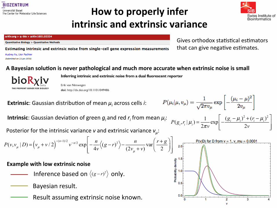
How to properly infer intrinsic and extrinsic variance
Gives orthodox sta0s0cal es0mators that can give nega0ve es0mates.
A Bayesian solu3on is never pathological and much more accurate when extrinsic noise is small
Extrinsic: Gaussian distribu0on of mean μi across cells i: Intrinsic: Gaussian devia0on of green gi and red ri from mean μi: P(gi ,ri | µi ) =
12πv
exp −(gi − µi )
2 + (ri − µi )2
2v⎡
⎣⎢⎢
⎤
⎦⎥⎥Posterior for the intrinsic variance v and extrinsic variance vμ:
P(v,vµ |D) = vµ + v / 2( )−(n−1)/2 v−n/2 exp − n4v
(g − r)2 − n(2vµ + v)
varr + g2
⎛⎝⎜
⎞⎠⎟
⎡
⎣⎢⎢
⎤
⎦⎥⎥
Example with low extrinsic noise
Inference based on only. (g − r)2
Bayesian result.
Result assuming extrinsic noise known.

Extrinsic noise implies transcrip3on/transla3on/decay rates fluctuate
Extrinsic noise in Elowitz et al: Intrinsic noise falls as the promoter is induced. Extrinsic noise peaks at intermediate induc0on.
R Phillips (Annu Rev Con Mat Phys, 2015)
• Transcrip0on rate can vary when the promoter switches between different states.
• Switching rates depend on concentra0ons of DNA binding proteins (polymerases, TFs).
• These concentra0ons will fluctuate from cell
to cell.

Noise propaga3on
• Regulatory cascade: Gene 1 induces gene 2. Gene 3 cons0tu0ve. • As gene 1 is induced, its own noise level drops. • Gene 2 goes through an intermediate peak in noise level. • Gene 3’s noise is unaffected. Interpreta3on: At intermediate levels of gene 1, the promoter of gene 2 shows most switching between bound and unbound states and most sensi0vity to fluctua0ons in the concentra0on of gene 1.

Cells are not sta3c: Inves0ga0ng stochas0c regulatory dynamics
Wish list • Follow growth and gene expression dynamics in single cells over long 0me scales. • Accurate quan0fica0on. • Follow different cell lineages separately to allow observa0on of rare events. • Precise dynamical control over growth environment.
Wang et al. Robust growth of Escherichia coli. Curr Biol. 2010
The mother machine

Our extension: The Dual Input Mother Machine

Switching growth media between glucose and lactose
• GFP/lacZ fusion reports lac-‐operon expression. • Switch glucose/lactose every 4 hours. • Immediate growth arrest at first switch to lactose. • Stochas0c induc0on of lac-‐operon and restart of growth. • Dilu0on of GFP/lacZ during glucose phase. • No more growth arrests upon later switches.

Automated Image Analysis: The Mother Machine Analyzer
Florian Jug Gene Myers
MPI Cell Biology, Dresden
• Tracking and segmenta0on done in parallel using a single objec0ve func0on.
• Interac3ve cura3on: • User input interpreted as addi0onal constraints. • Automa0c re-‐op0miza0on.

Cells expand exponen3ally during their cell cycle
2
34
2
34
2
34
2
34
0 4 8 12 16 20time (h)
cell
leng
th (µ
m)
0.970 0.975 0.980 0.985 0.990 0.995 1.0000.0
0.2
0.4
0.6
0.8
1.0
Pearson correlation exp. growth curve
FractionCellCycles
Cumula3ve correla3on coeff. of log(size) vs 3me
Example growth dynamics of log-‐size vs 3me
Roughly two-‐fold variability in growth rates

Fluorescence roughly tracks cell size but produc3on fluctuates significantly
Approximately 4-‐fold varia3on in produc3on rate
Examples of total fluorescence against 0me for single cells growing in
lactose.
Distribu0on of GFP molecules produced per second.

Distribu3on of total fluorescence and fluorescence concentra3ons
5000 10000 15000 20000 25000 30000 350000.00000
0.00005
0.00010
0.00015
Fluorescence HAUL
Probabilitydensity
Total Fluorescence Distribution
m=10'616, s=2911, sêm=0.274
8.5 9.0 9.5 10.0 10.50.0
0.2
0.4
0.6
0.8
1.0
1.2
1.4
Log Fluorescence HAUL
Probabilitydensity
Total Log Fluorescence Distribution
m=9.23,s2=0.07
4000 6000 8000 10000 120000.0000
0.0002
0.0004
0.0006
0.0008
Fluorescence concentrationHAUêmicronL
Probabilitydensity
Fluorescence Concentration Distribution
m=4278, s=661, sêm=0.154
8.0 8.5 9.0 9.50.0
0.5
1.0
1.5
2.0
2.5
3.0
Log Fluorescence concentrationHAUêmicronL
Probabilitydensity
Log Fluorescence Concentration Distribution
m=8.35,s2=0.022
Very roughly log-‐normal distribu0ons. Concentra0on has significantly less varia0on.

Measuring transcrip3on from all E. coli promoters in single cells
• GFP fluorescence per cell propor0onal to protein number.
• GFP levels of single cells can be measured in high-‐throughput using FACS.
• Quan0ta0vely characterize the distribu0on of expression levels across single cells, for all E. coli promoters.
ORF1 ORF2 ORF4 E. coli genome ORF3
Plasmid Zaslaver et al.
2006
Silander et al. PLoS genet 2012 Wolf et al. eLife 2015

FACS: Measuring and selec3ng single cells
• Cells move one-‐by-‐one in a flow channel.
• Each cell passes in front of a laser and its fluorescence is measured.
• By selec0vely charging par0cles based on their measured
fluorescence, one can select cells whose fluorescence lies in a certain range.

Gene expression distribu3ons for two example promoters
µ1 µ2
σ1σ 2
Promoter 1 Promoter 2

Means and variances of na3ve E. coli promoters
• Variance in log-‐expression in shows a trend of decreasing with mean expression.
• Different promoters with same mean can show significantly different variance.
• There seems to be a clear lower bound on variance as a func0on of mean.
5 6 7 8 9 10 110.0
0.2
0.4
0.6
0.8
Mean Log@GFP IntensityD
VarianceLog@G
FPpercellD
background
2 * background

7 8 9 10 11 12 130.0
0.2
0.4
0.6
0.8
Mean Log@proteins per cellD
VarianceLog@pr
oteins
percellD
7 8 9 10 11 12 130.0
0.2
0.4
0.6
0.8
Mean Log@ proteins per cellsD
Excess
noise
Means and variances of na3ve E. coli promoters
Red curve:
σ ab2 = 0.025, b = 450
n = ab, var(n) = (b+1) nAt constant transcrip0on/transla0on/decay rates: Assume a and b both fluctuate: var(n) = (b+1) n +σ ab
2 n2
nmeas = nbg + n + ε var(n) var log(nmeas )⎡⎣ ⎤⎦ =σ ab2 1−
nbgnmeas
⎛
⎝⎜
⎞
⎠⎟
2
+ (b+1)nmeas
1−nbgnmeas
⎛
⎝⎜
⎞
⎠⎟

Noise levels vary across na3ve E. coli promoters
7 8 9 10 11 12 130.0
0.2
0.4
0.6
0.8
Mean Log@proteins per cellD
VarianceLog@pr
oteins
percellD
7 8 9 10 11 12 130.0
0.2
0.4
0.6
0.8
Mean Log@ proteins per cellsD
Excess
noise
Excess noise (variance – lower bound as func. mean)
Selec3on on noise levels
High noise DriZ? Selected for noise?
Low noise. Selec0on to minimize noise?
What noise would one get without selec3on? Evolve synthe8c promoters in a precisely controlled selec0ve environment.

Directed evolu0on of promoters that express at a desired level
* * *
28

29
Evolu0on of popula0on expression levels
Selec0ng for Medium expression
29
Selec0ng for High expression

Expression distribu0ons of individual synthe0c promoters
• We isolated ~400 clones from evolu0onary runs for both medium and high expression. • Measured each clone’s expression distribu0on.
How do noise levels of synthe3c promoters compare with those of na3ve promoters?

Na0ve promoters Synthe0c promoters
• Synthe0c promoters were not selected on their noise proper0es. • Low noise is the default behavior of E. coli promoters. • Selec0on must have acted so as to increase the noise levels of some na0ve promoters.
Iden0cal distribu0ons at the low noise end.
High noise enriched in na0ve promoters.
Selec0on caused increased noise in a substan0al frac0on na0ve promoters
What is `special’ about na3ve promoters that show high noise?

Noisy genes have more regulatory inputs
• 185 E. coli transcrip0on factors (TFs). • 4123 known regulatory interac0ons TF → promoter.
Genes with higher noise have (on average) higher numbers of known regulatory inputs.
2 or more inputs 1 known input no known inputs synthe0c proms.
Why is there a general associa3on between noise and regula3on? Why did selec3on cause noise to increase?

Noise-‐propaga3on: nuisance or opportunity?
Noise as an unavoidable side-‐effect of regula3on • Explains the general associa0on of noise and regula0on. • `Fluctua0on-‐dissipa0on rela0on’: Genes that need complex regula0on unavoidably couple
to the noise in their regulators. • Generally assumed to be detrimental: reduces the accuracy of regula0on.
Stochas3city as a bet-‐hedging strategy • Phenotypic diversity can generally be selected for in fluctua0ng environments.
• Maybe noise-‐propaga0on can be beneficial in some circumstances?
Let’s do some theory on how gene expression noise affects fitness

Fitness func0on in a single environment
f (x |µ*,τ ) = exp −(x −µ*)
2
2τ 2"
#$
%
&'
p(x |µ,σ ) = 12πσ
exp −(x −µ)2
2σ 2
"
#$
%
&'
f (µ,σ |µ*,τ ) = dxp(x |µ,σ ) f (x |µ*,τ ) =∫ τ 2
τ 2 +σ 2 exp −(µ −µ*)
2
2(τ 2 +σ 2 )#
$%
&
'(
The fitness of a promoter `genotype’ (frac0on of its cells selected) is a convolu0on of these two func0ons (approx. area on the intersec0on):
Fitness (probability to be selected):
Promoter expression distribu0on:
σ = 0.1
µ µ*
τ

Moving the mean toward the desired level always increases fitness
f (µ,σ |µ*,τ ) =τ 2
τ 2 +σ 2 exp −(µ −µ*)
2
2(τ 2 +σ 2 )"
#$
%
&'
7.7 7.8 7.9 8.0 8.1 8.2 8.3 8.40.0
0.2
0.4
0.6
0.8
1.0
Log expression
ExpressionêSe
lectionprobability
7.7 7.8 7.9 8.0 8.1 8.2 8.3 8.40.0
0.2
0.4
0.6
0.8
1.0
Log expression
ExpressionêSe
lectionprobabilityf (µ = 8.0,σ = 0.1) = 0.066 f (µ = 8.1,σ = 0.1) = 0.174

7.7 7.8 7.9 8.0 8.1 8.2 8.3 8.40.0
0.2
0.4
0.6
0.8
1.0
Log expression
ExpressionêSe
lectionprobability
7.7 7.8 7.9 8.0 8.1 8.2 8.3 8.40.0
0.2
0.4
0.6
0.8
1.0
Log expression
ExpressionêSe
lectionprobability
At op0mal mean minimal noise is preferred
f (µ,σ |µ*,τ ) =τ 2
τ 2 +σ 2 exp −(µ −µ*)
2
2(τ 2 +σ 2 )"
#$
%
&'
f (µ = 8.15,σ = 0.1) = 0.196 f (µ = 8.15,σ = 0.025) = 0.625

As mean moves away from the op0mum there is a bifurca0on to nonzero op0mal noise
f (µ,σ |µ*,τ ) =τ 2
τ 2 +σ 2 exp −(µ −µ*)
2
2(τ 2 +σ 2 )"
#$
%
&'
f (µ = 8.0,σ = 0.05) = 0.0077
7.7 7.8 7.9 8.0 8.1 8.2 8.3 8.40.0
0.2
0.4
0.6
0.8
1.0
Log expression
ExpressionêSe
lectionprobability f (µ = 8.0,σ = 0.1) = 0.066
7.7 7.8 7.9 8.0 8.1 8.2 8.3 8.40.0
0.2
0.4
0.6
0.8
1.0
Log expression
ExpressionêSe
lectionprobability
`Bifurca3on’ in op3mal σ When , the op0mal noise level is non-‐zero:
0.0 0.2 0.4 0.6 0.8 1.00.0
0.2
0.4
0.6
0.8
1.0
Expression deviation »mu-mu*»
Optimalsigm
a
Op3mal σ
σ * = (µ −µ*)2 −τ 2
τ = 0.05
τ = 0.2µ −µ* ≥ τ

Variable environment: Fitness of an unregulated gene
log f (µ,σ )[ ] = −(µ −µe )
2
2(τ 2 +σ 2 )+12log τ 2
τ 2 +σ 2
"
#$
%
&'Log-‐fitness in a variable environment:
Assuming no regula0on, op0mal mean equals Log-‐fitness becomes: Op3mal noise matches the varia3on in desired expression levels:
log f (µ,σ )[ ] = − var(µe )2(τ 2 +σ 2 )
+12log τ 2
τ 2 +σ 2
"
#$
%
&'
This is the bet hedging scenario. But: Wouldn’t it be be\er to evolve gene regula0on?
σ opt2 = var(µe )−τ
2
µ = µe

Effects of coupling a gene to a regulator
Regulator’s ac0vity
Gene coupled to the regulator.
Gene without regula0on
TF
TF
Two main effects on the gene’s expression: 1. Condi3on-‐response: Mean depends on regulator’s (condi0on-‐dependent) ac0vity. 2. Noise-‐propaga3on: Noise increases due to propaga0on of the regulator’s noise.
We developed a general theory to calculate how these effects conspire to affect fitness.

Fitness depends on only 4 effec3ve parameters Varia0on in desired levels: V
στ1. Expression mismatch: Y 2 = V
σ 2 +τ 2
Varia0on in regulator levels: Vr
σ r
2. Signal-‐to-‐noise of the regulator: S 2 = Vrσ r2
3. Correla3on regulator/desired levels: R
Fitness effect of the regulatory interac3on:
4. Coupling strength: X
log[ f ]= − 12
Y 2 (1− R2 )+ SX − RY( )2
(1+ X 2 )−12log 1+ X 2"
#$%
Scenario: Start with unregulated promoter. What fitness can be obtained by coupling to regulator with signal-‐to-‐noise S and correla0on R?

Fitness with op0mal coupling to a regulator of given correla0on R and signal-‐to-‐noise S
Fitness of the unregulated promoter.
Y=4 Perfect
correla0on
No correla0on
Noisy regulator
Precise regulator

Coupling to a near op3mal regulator: condi3on-‐response effect
Y=4
TF TF
σ tot = 0.16R = 0.95S = 3.3
Fitness of the unregulated promoter.

Coupling to a noisy uncorrelated regulator: noise-‐propaga3on implements bet hedging strategy
Y=4
TF TF
σ tot = 0.55
R = 0S = 0.19
Fitness of the unregulated promoter.

Intermediate case: a moderately correlated regulator
Y=4
TF TF
σ tot = 0.23
R = 0.64S = 2.45
Fitness of the unregulated promoter.

Op0mal S at a given R.
Y=4
Condi3on-‐response and noise-‐propaga3on typically act in concert
Regulator too noisy.
Regulator not noisy enough.
• Noise-‐propaga0on is oZen func8onal, ac0ng as a rudimentary form of regula0on.
• De novo evolu0on of regula0on: Star0ng from pure noise-‐propaga0on (R=0,S=0) there is a con0nuum of solu0ons of increasing accuracy along which condi0on-‐response and noise-‐propaga0on op0mally complement each other.
• Regulated genes are noisy because, whenever the condi0on-‐response is imperfect,
maximal fitness requires noisy regulators.
Summary Theory:

0 1 2 3 4 5 60.0
0.2
0.4
0.6
0.8
1.0
Y: Expression mismatch
R:Co
rrelation
ofregulator'sexpressio
nwithdesired-levels σ tot
2 =σ 2
Low noise regime: Promoters with low expression mismatch Y<1 `do not bother’ to be regulated. For extremely correlated regulators, zero noise-‐propaga0on is the op0mum.
Phase diagram of final noise aZer coupling to regulators with op0mal noise levels.

0 1 2 3 4 5 60.0
0.2
0.4
0.6
0.8
1.0
Y: Expression mismatch
R:Co
rrelation
ofregulator'sexpressio
nwithdesired-levels σ tot
2 =σ 2
Noise-‐propaga3on regime: The final noise level matches the frac0on of variance in desired levels not tracked by the condi0on-‐response.
σ tot2 = (1− R2 )var(µe )−τ
2
Phase diagram of final noise aZer coupling to regulators with op0mal noise levels.
Amount of regula3on required. Variance in desired levels
Selec3on tolerance
Limited accuracy of the condi3on-‐response. Frac3on variance not tracked by regula3on.

Conclusions
signal
regulator
• We evolved synthe0c promoters de novo in E. coli under carefully-‐controlled selec0ve condi0ons.
• No evidence E. coli promoters have been selected to lower noise. • Regulated genes have been selected to increase noise.
Experimental observa3ons
Theory • Coupling a regulator to a target promoter has two effects:
1. Condi0on-‐response. 2. Noise-‐propaga0on.
• Noise-‐propaga0on alone can act as a rudimentary form of regula0on. • Accurate regula0on can evolve smoothly along a con0nuum in which
noise-‐propaga0on and condi0on-‐response act in concert. • Whenever the condi0on-‐response has limited accuracy, noisy
regula0on is preferred. • Explains the general associa0on between noise and regula0on.
Thank you!
Luise Wolf Olin Silander
Theory/computa3on PhD and post-‐doc posi3ons available!
This work: Our group