geir storvik ch 7 - markov chain monte carlo

STK4051/9051 Computational statistics

Geir Storvik

Ch 7 - Markov chain Monte Carlo

Geir Storvik STK4051/9051 Computational statistics 1 / 42 Ch 7 - Markov chain Monte Carlo 1 / 42

Markov chain Monte Carlo

Assume now simulating from f (X) is difficult directlyf (·) complicatedX high-dimensional

Markov chain Monte Carlo:Generates {X(t)} sequentiallyMarkov structure: X(t) ∼ P(·|X(t−1))

Aim now:The distribution of X(t) converges to f (·) as t increasesµ̂MCMC = N−1∑N

t=1 h(X(t)) converges towards µ = E f [h(X)] as t increases


Markov chain theory - discrete case

Assume {X (t)} is a Markov chain where X (t) is a discrete random variable

Pr(X (t) = y |X (t−1) = x) = P(y |x)

giving the transition probabilitiesAssume the chain is

irreducible: It is possible to move from any x to any y in a finite number of stepsreccurent: The chain will visit any state infinitely often.aperiodic: Does not go in cycles

Then there exists a unique distribution f (x) such that

limt→∞

Pr(X (t) = y |X (0) = x) =f (y)

µ̂MCMC →µ = E f [X ]

How to find f (·) (the stationary distribution): Solve

f (y) =∑

x

f (x)P(y |x)

Our situation: We have f (y), want to find P(y |x)

Note: Many possible P(y |x)!


Markov chain theory - general setting

Assume {X(t)} is a Markov chain where X(t) ∈ S

Pr(X(t) ∈ A|X(t−1) = x) = P(x,A) =

∫y∈A

P(y|x)dy

giving the transition densitiesAssume the chain is

irreducible: It is possible to move from any x to any y in a finite number of stepsreccurent: The chain will visit any A ⊂ S infinitely often.aperiodic: Do not go in cycles

Then there exists a distribution f (x) such that

limt→∞

Pr(X(t) ∈ A|X(0) = x) =

∫A

f (y)dy

µ̂MCMC →µ

How to find f (·) (the stationary distribution): Solve

f (y) =

∫x

f (x)P(y|x)dx

Our situation: We have f (·), want to find P(y|x)


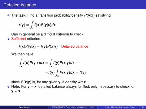
Detailed balance

The task: Find a transition probability/density P(y|x) satisfying

f (y) =

∫x

f (x)P(y|x)dx

Can in general be a difficult criterion to checkSufficient criterion:

f (x)P(y|x) = f (y)P(x|y) Detailed balance

We then have∫x

f (x)P(y|x)dx =

∫x

f (y)P(x|y)dx

=f (y)

∫x

P(x|y)dx = f (y)

since P(x|y) is, for any given y, a density wrt x.Note: For y = x, detailed balance always fulfilled, only necessary to check fory 6= x.


Metropolis-Hastings algorithms

P(y|x) defined through an algorithm:1 Sample a candidate value X∗ from a proposal distribution g(·|x).2 Compute the Metropolis-Hastings ratio

R(x,X∗) =f (X∗)g(x|X∗)f (x)g(X∗|x)

3 Put

Y =

{X∗ with probability min{1,R(x,X∗)}x otherwise

For y 6= x:

P(y|x) = g(y|x) min

{1,

f (y)g(x|y)

f (x)g(y|x)

}Note: P(x|x) somewhat difficult to evaluate in this case.Detailed balance (?)

f (x)P(y|x) =f (x)g(y|x) min

{1,

f (y)g(x|y)

f (x)g(y|x)

}= min{f (x)g(y|x), f (y)g(x|y)}

=f (y)g(x|y) min

{f (x)g(y|x)

f (y)g(x|y), 1}

= f (y)P(x|y)


Example

Assume f (x) ∝ exp(−|x |3/3)

Proposal distribution N(x , 1)

Example_MH_cubic.R


Independent chains

Assume g(x∗|x) = g(x∗). Then

R(x, x∗) =f (x∗)g(x)

f (x)g(x∗)=

f (x∗)g(x∗)f (x)g(x)

,

fraction of importance weights!

Behave very much like importance sampling and SIR

Difficult to specify g(x) for high-dimensional problems

Theoretical properties easier to evaluate than for random walk versions.


M-H and multivariate settings

X = (X1, ...,Xp)

Typical in this case: Only change one or a few components at a time.1 Choose index j (randomly)2 Sample X ∗j ∼ gj (·|x), put X ∗k = Xk for k 6= j3 Compute

R(x,X∗) =f (X∗)g(x|X∗)f (x)g(X∗|x)

4 Put

Y =

{X∗ with probability min{1,R(x,X∗)}x otherwise

Can show that this version also satisfies detailed balanceCan even go through indexes systematic

Should then consider the whole loop through all components as one iteration


Example

Assume f (x) ∝ exp(−||x||3/3) = exp(−[||x||2]3/2/3) =

Proposal distribution1 j ∼ Uniform[1, 2, ..., p]2 x∗j ∼ N(xj , 1)

Example_MH_cubic_multivariate.R


Reparametrization

Sometimes easier to transform variables to another scale Y = h̄(X )

Two approaches (use h−1(·) = h̄(·) so X = h(Y ))Reparametrize Y = h̄(X), simulate from fY (y) instead

fY (y) =fX (h(y))|h′(y)|

R(y , y∗) =fX (h(y∗))|h′(y∗)|gy (y |y∗)fX (h(y))|h′(y)|gy (y∗|y)

=fX (x∗)|h′(y∗)|gy (y |y∗)fX (x)|h′(y)|gy (y∗|y)

Run the MCMC in X -space, but construct proposal through X = h(Y ),

gx (x∗|x) =gy (h̄(x∗)|h̄(x))|h̄′(x∗)|

R(x , x∗) =fX (x∗)gy (h̄(x)|h̄(x∗))|h̄′(x)|fX (x)gy (h̄(x∗)|h̄(x))|h̄′(x∗)|

=fX (x∗)gy (y |y∗)|h′(y∗)|fX (x)gy (y∗|y)|h′(y)|

since h̄′(x) = 1/h′(y)


Gibbs sampling

Assume X = (X1, ...,Xp)

Aim: Simulate X ∼ f (x)

Gibbs sampling:1 Select starting values x(0) and set t = 02 Generate, in turn

X (t+1)1 ∼f (x1|x

(t)2 , x (t)

3 , ..., x (t)p )

X (t+1)2 ∼f (x2|x

(t+1)1 , x (t)

3 , ..., x (t)p )

...

X (t+1)p−1 ∼f (xp−1|x

(t+1)1 , ..., x (t+1)

p−2 , x (t)p )

X (t+1)p ∼f (xp|x (t+1)

1 , ..., x (t+1)p−1 )

3 Increment t and go to step 2.

Completion of step 2 is called a cycle


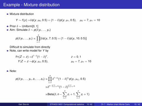
Example - Mixture distribution

Mixture distribution

Y ∼ f (y) =δφ(y , µ0, 0.5) + (1− δ)φ(y , µ1, 0.5), µ0 = 7, µ1 = 10

Prior δ ∼ Uniform[0, 1]Aim: Simulate δ ∼ p(δ|y1, ..., yn)

p(δ|y1, ..., yn) ∝n∏

i=1

[δφ(yi , 7, 0.5) + (1− δ)φ(yi , 10, 0.5)]

Difficult to simulate from directlyNote, can write model for Y by

Pr(Z = z) =δ1−z(1− δ)z , z = 0, 1

Y |Z = z ∼φ(y , µz , 0.5), µ0 = 7, µ1 = 10

Note:

p(δ|y1, ..., yn, z1, ..., zn) ∝n∏

i=1

δ1−zi (1− δ)ziφ(yi , µzi , 0.5)

∝δn−∑n

i=1 zi (1− δ)∑n

i=1 zi

∝Beta(δ, n −n∑

i=1

zi + 1,n∑

i=1

zi + 1)


Example - continued

Aim: Simulate δ ∼ p(δ|y1, ..., yn)

Approach: Simulate from p(δ,Z|y1, ..., yn)Gibbs sampling

1 Initialize δ(0), set t = 02 Simulate Z(t+1) ∼ p(z|δ(t), y)3 Simulate δ(t+1) ∼ p(δ|z(t+1), y)4 Increment t and go to step 2.

Conditional distribution for z:

p(z|δ, y) ∝p(δ)p(z|δ)p(y|z, δ)

∝n∏

i=1

δ1−zi (1− δ)ziφ(yi , µzi , 0.5)

Independence between zi ’s:

Pr(Zi = zi |δ, yi ) ∝δ1−zi (1− δ)ziφ(yi , µzi , 0.5)

∝

{δφ(yi ,µ0,0.5)

δφ(yi ,µ0,0.5)+(1−δ)φ(yi ,µ1,0.5) zi = 0(1−δ)φ(yi ,µ1,0.5)

δφ(yi ,µ0,0.5)+(1−δ)φ(yi ,µ1,0.5) zi = 1

Mixture_Gibbs_sampler.R


Example - capture-recapture

Aim: Estimate population size, N, of a speciesProcedure:

At time t1: Catch c1 = m1 individuals, each with probability α1.Mark and releaseAt time ti , i > 1: Catch ci individuals, each with probability αi .Count number of newly caught individuals, mi , mark the unmarked and release all

Likelihood:At time t1:

Pr(C1 = c1) = Pr(C1 = m1) =( N

m1

)α

m11 (1− α1)N−m1

At time ti , i > 1 (number of marked individuals are∑i−1

k=1 mk )

Pr(Ci =ci ,Mj = mi |N, c1:i−1,m1:i−1)

= Pr(Ci = ci |N) Pr(Mi = mi |N,Ci = ci ,m1:i−1)

=(N

ci

)α

cii (1− αi )

N−ci

(N−∑i−1

k=1 mkmi

)(∑i−1k=1 mk

ci−mi

)(N

ci

)=α

cii (1− αi )

N−ci(N −

∑i−1k=1 mk

mi

)(∑i−1k=1 mk

ci −mi

)Geir Storvik STK4051/9051 Computational statistics 17 / 42 Ch 7 - Markov chain Monte Carlo 17 / 42

Example - capture-recapture - continued

Likelihood:

L(N,α|c,m) ∝( N

m1

)α

m11 (1− α1)N−m1×

I∏i=2

αcij (1− αi )

N−ci(N −

∑i−1k=1 mk

mi

)(∑i−1k=1 mk

ci −mi

)

∝I∏

i=1

αcii (1− αi )

N−ci(N −

∑i−1k=1 mk

mi

)

∝( N∑I

k=1 mk

) I∏i=1

αcii (1− αj )

N−ci

Prior:

f (N) ∝1

f (αi |θ1, θ2) ∼Beta(θ1, θ2)

Can derive (r =∑I

k=1 mk ):

N|α, c,m ∼r + NegBinom(r + 1, 1−I∏

i=1

(1− αi ))

αi |N,α−i , c,m ∼Beta(ci + θ1,N − ci + θ2)

Example_7_6.R


Properties of Gibbs sampler (random scan)

Gibbs sampling (random scan):1 Select starting values x(0) and set t = 02 Sample j ∼ Uniform{1, ..., p}3 Sample X (t+1)

j ∼ f (xj |x(t)−j )

4 Put X (t+1)k = X (t)

k for k 6= j

The chain {X(t)} is MarkovDetailed balance:

Consider x, x∗ where xj 6= x∗j while xk = x∗k for k 6= j

f (x)P(x∗|x) =f (x)p−1f (x∗j |x−j )

=f (x−j )f (xj |x−j )p−1f (x∗j |x−j )

=f (x∗−j )f (xj |x∗−j )p−1f (x∗j |x∗−j )

=f (x∗)p−1f (xj |x∗−j )

=f (x∗)P(x|x∗)


Properties of Gibbs sampler (deterministic scan)

Gibbs sampling (deterministic scan):1 Select starting values x(0) and set t = 02 Generate, in turn

X (t+1)1 ∼f (x1|x

(t)2 , x (t)

3 , ..., x (t)p )

X (t+1)2 ∼f (x2|x

(t+1)1 , x (t)

3 , ..., x (t)p )

...

X (t+1)p−1 ∼f (xp−1|x

(t+1)1 , ..., x (t+1)

p−2 , x (t)p )

X (t+1)p ∼f (xp|x (t+1)

1 , ..., x (t+1)p−1 )

3 Increment t and go to step 2.

The chain {X(t)} is Markov

Do not fulfill detailed balance (going backwards will revert order of componentsvisited)

Will still satisfy

f (x∗) =

∫x

f (x)P(x∗|x)dx


Tuning the Gibbs sampler

Random or deterministic scan?Deterministic scan most common (?)When high correlation, random scan can be more efficient

Blocking:When dividing X = (X1, ...,Xp), each Xj can be vectorsMaking each Xj as large as possible will typically improve convergenceEspecially beneficial when high correlation between single components

Hybrid Gibbs samplingIf f (xj |x−j ) is difficult to sample from, use an Metropolis-Hastings step for thiscomponentExample (p = 5)

1 Sample X (t+1)1 ∼ f (x1|x

(t)−1)

2 Sample (X (t+1)2 ,X (t+1)

3 ) through an M-H step3 Sample X (t+1)

4 through another M.H step4 Sample X (t+1)

5 ∼ f (x5|x(t+1)−5 )


Capture-recapture - extended approach

Assume now a prior f (θ1, θ2) ∝ exp{−(θ1 + θ2)/1000}Conditional distributions:

N|· ∼r + NegBinom(r + 1, 1−I∏

i=1

(1− αj ))

αi |· ∼Beta(ci + θ1,N − ci + θ2)

(θ1, θ2)|· ∼k[

Γ(θ1 + θ2)

Γ(θ1)Γ(θ2)

]I I∏i=1

αθ1i (1− αi )

θ2 exp{− θ1+θ2

1000

}Example_7_7.R


Convergence issues of MCMC

Theoretical properties:

X(t) D→ f (x), as t →∞

θ̂1 =1L

L∑t=1

h(X(t))→ E f [h(X)] as L→∞

Note: We also have

θ̂2 =1L

D+L∑t=D+1

h(X(t))→ E f [h(X)] as L→∞

Advantage: Remove those variables with distribution very different from f (x)Disadvantage: Need more samples

Question: How to specify D and L?D: Large enough so that X(t) ≈ f (x) for t > D (bias small)L: Large enough so that Var[θ̂2] is small enough


Mixing

For θ̂ = 1L

∑D+Lt=D+1 h(X(t)):

Var[θ̂] =1L2

[D+L∑

t=D+1

Var[h(X(t))] + 2D+L−1∑s=D+1

D+L∑t=s+1

Cov[h(X(s)), h(X(t))]

]

Assume D large, so "converged":

Var[h(X(t))] ≈ σ2h, Cov[h(X(s)), h(X(t))] ≈ σ2

hρ(t − s)

gives

Var[θ̂] ≈ 1L2

[D+L∑

t=D+1

σ2h + 2

D+L−1∑s=D+1

D+L∑t=s+1

σ2hρ(t − s)

]

=σ2

h

L

[1 + 2

L−1∑k=1

L− kL

ρ(k)

]

Good mixing: ρ(k) decreases fast with k !


Example from Exercise 7.8

Time

muM1[1:10000]

0 2000 4000 6000 8000 10000

2224

2628

30

0 10 20 30 40 50

0.0

0.2

0.4

0.6

0.8

1.0

Lag

ACF

Series muM1

Time

muM2[1:10000]

0 2000 4000 6000 8000 10000

2224

2628

30

0 10 20 30 40 50

0.0

0.2

0.4

0.6

0.8

1.0

Lag

ACF

Series muM2


How to assess convergence?

Graphical diagnostics:Sample paths:

Plot h(X(t)) as function of tUseful with different h(·) functions!

Cusum diagnosticsPlot

∑ti=1[h(X(i))− θ̂n] versus t

Wiggly and small excursions from 0: Indicate chain is mixing well

0e+00 2e+04 4e+04 6e+04 8e+04 1e+05

-10000

05000

1:N2

cum

sum

(muM

1) -

c(1:

N2)

* m

ean(

muM

1)

0e+00 2e+04 4e+04 6e+04 8e+04 1e+05

-400

-200

0100

1:N2

cum

sum

(muM

2) -

c(1:

N2)

* m

ean(

muM

2)


The Gelman-Rubin diagnostic

Motivated from analysis of variance

Assume J chains run in parallel

j th chain: x (D+1)j , ..., x (D+L)

j (first D discarded)

Define

x̄j =1L

D+L∑t=D+1

x (t)j x̄· =

1J

J∑j=1

x̄j

B =L

J − 1

J∑j=1

(x̄j − x̄·)2

W =1J

J∑j=1

s2j s2

j =1

L− 1

D+L∑t=D+1

(x (t)j − x̄j )

2

If converged, both B and W estimates σ2 = Varf [X ]

Diagnostic: R =L−1

L W + 1L B

W

"Rule":√

R < 1.1 indicate D and L are sufficient


Example: Exercise 7.8

D = 100, L = 1000:√

R1 = 1.588,√

R2 = 1.002,

D = 1000, L = 1000:√

R1 = 1.700,√

R2 = 1.004,

D = 1000, L = 10000:√

R1 = 1.049,√

R2 = 1.0008

0 2000 4000 6000 8000 10000

12

34

5

cbind(1:L, 1:L)

cbin

d(R

1, R

2)


Apparent convergence

f (x) = 0.7 · N(7, 0.52) + 0.3 · N(10, 0.52)Metropolis-Hastings with proposal N(x (t), 0.052)First 4000 samples (400 discarded)

Time

x.sim[1:4000]

0 1000 2000 3000 4000

910

1112

13

Full 10000 samples

Time

x.sim

0e+00 2e+04 4e+04 6e+04 8e+04 1e+05

68

1012


M-H: Choice of proposal distribution

Independence chain:g(·) ≈ f (·)High acceptance rateTail properties most important: f/g should be bounded

Random walk proposalTune variance so that acceptance rate is between 25 and 50%


Effective sample size for MCMC

For θ̂ = 1L

∑D+Lt=D+1 h(X(t)):

Var[θ̂] =σ2

h

L

[1 + 2

L−1∑k=1

L− kL

ρ(k)

]L→∞→ σ2

h

L[1 + 2

∞∑k=1

ρ(k)]

If independent samples:

Var[θ̂] =σ2

h

L

Effective sample size: L1+2

∑∞k=1 ρ(k)

Use empirical estimates ρ̂(k)

Usual to truncate the summation when ρ̂(k) < 0.1.


Number of chains

Assume possible to perform N iterationsOne long chain of length N, orJ parallel chains, each of length N/J?

Burnin:One long chain: Only need to discard D samplesParallel chains: Need to discard J · D samples

Check of convergenceEasier with many parallel chains

EfficiencyParallel chains give more independent samples

Computational issuesPossible to utilize multiple cores with parallel chains


Data uncertainty and Monte Carlo uncertainty

Parameter: θ = E f [h(X)]

Estimator: θ̂ = 1L

∑D+Lt=D+1 h(X(t)):

Two types of uncertaintyVariability in h(X): σ2

h = Varf [h(X)]

Estimator: σ̂2h = 1

L

∑D+Lt=D+1[h(X(t))− θ̂]2

MC variability in θ̂:Estimator: Divide data into batches of size b = bL1/ac, make estimates θ̂ within each batchand variance from these

Recommendation: Specify L so that MC variability is less than 5% of variability inh(X).


Advanced topics in MCMC

Adaptive MCMC: Automatic tuning of proposal distributionsMain challenge: Specifying proposal based on history of chain breaks down theMarkov propertySolution: Reduce the amount of tuning as the number of iterations increases

Reversible Jump MCMCAssume several modelsM1, ...,MKCorresponding parameters θ1, ..., θK of different dimensions!Aim: Simulate X = (M, θM)RJMCMC: M-H method for moving between spaces of different dimensionsMain challenge: When changingM→M∗, how to propose θM∗?

Simulated temperingDefine f i (x) ∝ f (x)1/τi , 1 = τ1 < τ2 < · · · < τmSimulate (X, I), where I changes distributionEasier to move around when τi > 1Keep samples for which I = 1

Multiple-Try M-HGenerate k proposals X∗1, ...,X

∗k from g(·|x(t))

Select X∗j with probability w(x(t),X∗j ) = f (x(t))g(X∗j |x(t))λ(x(t),X∗j ), λ symmetric

Sample X∗∗1 , ...,X∗∗k−1 from g(·|X∗j ), put X∗∗k = x(t)

Use Generalized M-H ratio

Rg =

∑ki=1 w(x(t),X∗i )∑ki=1 w(X∗j ,X

∗∗i )


Hamiltonian MC

Common trick in Monte Carlo: Introduce auxiliary variables

Hamiltonian MC (Neal et al., 2011):

π(q) ∝ exp(−U(q)) Distribution of interest

π(q,p) ∝ exp(−U(q)− 0.5pT p) Extended distribution

= exp(−H(q,p)) H(q,p) = U(q) + 0.5pT p

Noteq and p are independentp ∼ N(0, I).Usually dim(p)= dim(q)

Algorithm (q) current value1 Simulate p ∼ N(0, I)2 Generate (q∗,p∗) such that H(q∗,p∗) ≈ H(q,p)3 Accept (q∗,p∗) by a Metropolis-Hastings step

Main challenge: Generate (q∗,p∗)


Hamiltonian dynamics

Consider (q,p) as a time-process (q(t),p(t))

Hamiltonian dynamics: Change through

dqi

dt=∂H∂pi

dpi

dt=− ∂H

∂qi

This gives

dHdt

=

d∑i=1

[∂H∂qi

dqi

dt+∂H∂pi

dpi

dt

]

=

d∑i=1

[∂H∂qi

∂H∂pi− ∂H∂pi

∂H∂qi

]= 0

If we can change (q,p) exactly by the Hamiltonian dynamics, H will not change!

In practice, only possible to make numerical approximations


Hamiltonian dynamics - Eulers method

Assume

pi (t + ε) =pi (t) + εdpi

dt(t)

=pi (t)− ε∂U∂qi

(qi (t))

qi (t + ε) =qi (t) + εdqi

dt(t)

=qi (t) + εpi (t)

Note: Derivatives of U(q) are used.

However, not very exact. −2.0 −1.5 −1.0 −0.5 0.0 0.5 1.0−

10

12

q

p


Hamiltonian dynamics - the modified Eulers method

Assume

pi (t + ε) =pi (t)− ε∂U∂qi

(q(t))

qi (t + ε) =qi (t) + εpi (t + ε)

Better than Eulers method.

−1.0 −0.5 0.0 0.5 1.0−

1.0

−0.

50.

00.

51.

0

q

p


Hamiltonian dynamics - the Leapfrog method

Assume

pi (t + ε2 ) =pi (t)−

ε

2∂U∂qi

(q(t))

qi (t + ε) =qi (t) + εpi (t + ε2 )

pi (t + ε) =pi (t + ε2 )− ε

2∂U∂qi

(q(t + ε))

Quite exact!

Idea: Use this L steps −1.0 −0.5 0.0 0.5 1.0−

1.0

−0.

50.

00.

51.

0q

p


Example - 2-dimensional Gaussian

Assume x ∼ N(0,ΣΣΣ), ΣΣΣ =

(1 0.95

0.95 1

)H(x ,p) = 0.5xT ΣΣΣ−1x + 0.5pT p

Use L = 5 leapfrog steps, with stepsize ε = 0.1

leapfrog_Gauss2.R


Example - mixture Gaussians

Assume

π(x) = pN(x ;µ1, σ21) + (1− p)N(x ;µ2, σ

22)

H(x ,p) = −log(π(x) + 0.5pT p

Use L = 5 leapfrog steps, with stepsize ε = 0.1

leapfrog_mixture.R


R. M. Neal et al. MCMC using Hamiltonian dynamics. Handbook of Markov ChainMonte Carlo, 2(11):2, 2011.


geir storvik ch 7 - markov chain monte carlo

Documents