GEARS: A General and Efficient Algorithm for Rendering Shadows

Voicu Popescu

1

Reference

• GEARS.pdf

• GEARS.mov

2

3

Fig. 1: Soft shadows rendered with our method (left for each pair) and with ray tracing (right for each pair), for comparison. The average frame rate for our method vs. ray tracing is 15.7fps vs. 0.5fps for the Bird Nest scene and 32.7fps vs. 2.7fps for the Spider scene.

Shadows

• Important effect in graphics

• Difficult to render

– Require estimating visibility from light source

4

Hard shadows

• Point light sources

• Usually rendered using shadow mapping

– Z-buffer rendered from light point

– Output sample unprojected to 3-D then projected to shadow map

– Inaccurate when shadow map texel is magnified in output image

5

Pixel-accurate hard shadows

• Render scene from output view, w/o shadows

• Unproject/re-project output image samples to shadow plane

• Define grid on shadow plane

• Assign output image samples to grid cells

• Render scene from light; For all triangles t • Project t onto grid to t’

– For all grid cells c touched by t’

» For all output samples s in c

• Mark s as in shadow if covered by t’ 6

Soft shadows

• Area light source

• Umbra (full shadow), penumbra (in between), and light regions

• Computationally expensive

– Estimating visibility from light source requires many rays

7

Soft shadows approaches

• Trace k x k rays for each pixel – Ray tracing is expensive, HW unfriendly, acceleration

difficult, especially for dynamic scenes

• Construct k x k conventional shadow maps – Expensive to render scene k x k times

– Approximation errors of conventional shadow maps

• Render scene at k x k resolution for each output image sample – Approach taken by our technique

• k should be at least 16

8

Algorithm overview

9

Fig. 2: Soft shadow computation overview for light L0L1, output image I0I1 with viewpoint E, blocker B0B1, and receiver R0R1.

Acceleration scheme

10

Fig. 3: Camera used to define and populate grid.

Acceleration scheme

11

Fig. 4: Top: projection of shadow volume of triangle B0B1B2 onto 2-D grid with axes xG and yG. Bottom: 2-D AABB Q0Q1Q2Q3 is a tight approximation of the shadow volume projection.

12

Fig.5: Pixel sample and triangle assignment to grid.

Acceleration scheme

Results: quality

13

Results: quality

14

Fig. 7: Additional scenes used to test out method.

Results: performance

15

Results: performance

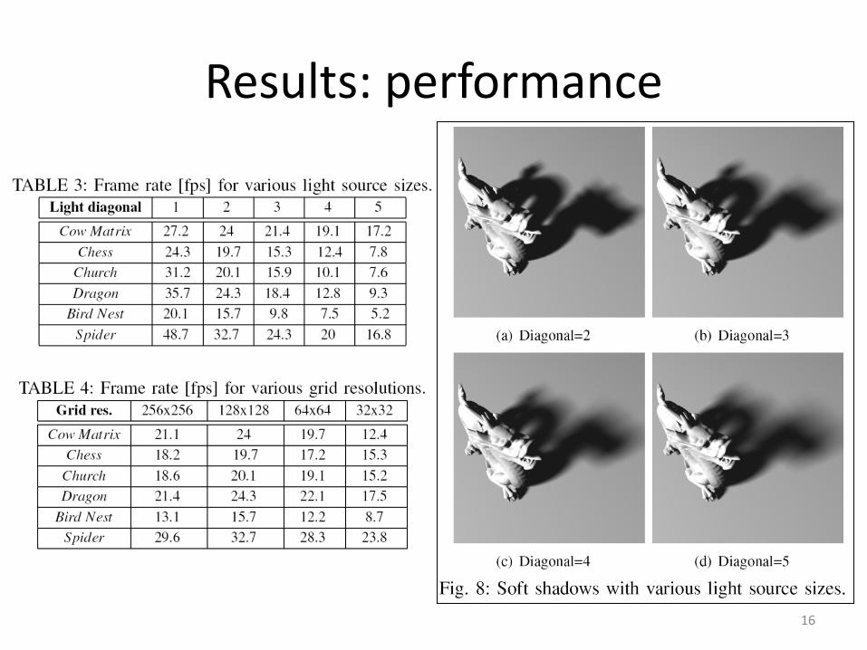
16

Results: performance

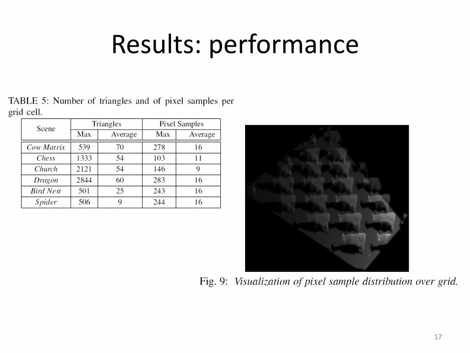
17

Results: performance

18

Results: performance

19

Performance: comparison to ray tr’ng

20

Performance: comparison to ray tr’ng

21