gaussian kernel width optimization for sparse bayesian learning

This article has been accepted for inclusion in a future issue of this journal. Content is final as presented, with the exception of pagination.

IEEE TRANSACTIONS ON NEURAL NETWORKS AND LEARNING SYSTEMS 1

Gaussian Kernel Width Optimization forSparse Bayesian Learning

Yalda Mohsenzadeh and Hamid Sheikhzadeh, Senior Member, IEEE

Abstract— Sparse kernel methods have been widely used inregression and classification applications. The performance andthe sparsity of these methods are dependent on the appro-priate choice of the corresponding kernel functions and theirparameters. Typically, the kernel parameters are selected usinga cross-validation approach. In this paper, a learning methodthat is an extension of the relevance vector machine (RVM)is presented. The proposed method can find the optimal val-ues of the kernel parameters during the training procedure.This algorithm uses an expectation–maximization approach forupdating kernel parameters as well as other model parameters;therefore, the speed of convergence and computational complexityof the proposed method are the same as the standard RVM. Tocontrol the convergence of this fully parameterized model, theoptimization with respect to the kernel parameters is performedusing a constraint on these parameters. The proposed method iscompared with the typical RVM and other competing methodsto analyze the performance. The experimental results on thecommonly used synthetic data, as well as benchmark data sets,demonstrate the effectiveness of the proposed method in reducingthe performance dependency on the initial choice of the kernelparameters.

Index Terms— Adaptive kernel learning (AKL), expecta-tion maximization (EM), kernel width optimization, regression,relevance vector machine (RVM), sparse Bayesian learning,supervised kernel methods.

I. INTRODUCTION

IN REGRESSION problems, a set of input and targetobservations {xn, tn}N

n=1 is given. The target value tn ∈ Ris considered as a noisy output of a function y(xn) of inputvector xn ∈ RM as

tn = y(xn) + εn (1)

where εn is a measurement noise corresponding to the nthinput–output observation. The regression framework opts toestimate the function y(xn) based on the observations (trainingdata). Consequently, using this estimated function, the predic-tion of the target value t∗ for x∗, a new arbitrary test input, ispossible [1]. Sparse kernel-based methods typically assume alinearly weighted model for y(x) as

y(x|w) = w0 +N∑

n=1

wn K (x, xn) (2)

Manuscript received May 28, 2013; revised April 18, 2014; acceptedApril 20, 2014.

The authors are with the Department of Electrical Engineering,Amirkabir University of Technology, Tehran 14158-54546, Iran (e-mail:[email protected]; [email protected]).

Digital Object Identifier 10.1109/TNNLS.2014.2321134

where w = [w0, w1, . . . , wN ]T is the weight vector of thelinear model and K (x, xn) is a predetermined kernel functioncentered on the training sample xn [1], [2]. The goal is todetermine a sparse solution for the weight vector w in thelinear model of (2) using the training data. However, since thenumber of unknown weights and the training samples are thesame, solving (2) will not yield a sparse model and overfit-ting to the training data is inevitable. Tipping [3] proposedthe relevance vector machine (RVM), a Bayesian learningapproach, to find the desired sparse model. The RVM imposesprior distributions over the weights and hyperparameters suchthat the marginalized prior over the weights results in asparse model. Specifically, in the sparse Bayesian learning,considering a zero-mean Gaussian prior distribution with aseparate variance for each weight and a flat gamma priordistribution on the hyperparameters (variances of Gaussiandistributions over the weights), a student-t marginalized priordistribution over weights is resulted. Therefore, a sparse modelis obtained using the RVM to learn the parameters. TheRVM learned model is dependent only on a subset of trainingsamples known as relevance vectors (RVs).

Note that the RVM assumes that the kernel functionsare predetermined. Consequently, although RVM has demon-strated a promising performance in many applications com-pared with other learning methods [4]–[11], its efficiency andsparsity are highly dependent on the choice of an appropri-ate kernel function. Typically, the parameters of the kernelfunction are achieved using a cross-validation approach in thetraining stage. In general, there is no limitation on the choiceof kernel function in the RVM model; however, the Gaussiankernel also known as radial basis function (RBF) is the mostpopular and widely used kernel function for the standard RVM.In the standard RVM, this kernel function is defined as

Kstd(x, xn) = exp

{−‖x − xn‖2

2b2

}for n = 1, ..., N (3)

where b is the kernel width and N is the number of trainingsamples. Note that the kernel width is invariant for all trainingsamples in the standard RVM. Therefore, for a data set thatconsists of noisy samples of a function with time-varyingdynamics (e.g., Doppler signal or speech signals), choosinga large kernel width will result in a predicted RVM response,which is smoothed in the high-frequency subdomains of thedynamic function. On the other hand, selecting a small kernelwidth will yield a predicted RVM response, which is over-fitted in the low-frequency subdomains of the dynamic func-tion [12], [13]. Recently, to tackle this problem, [12] and [13]

2162-237X © 2014 IEEE. Personal use is permitted, but republication/redistribution requires IEEE permission.See http://www.ieee.org/publications_standards/publications/rights/index.html for more information.


2 IEEE TRANSACTIONS ON NEURAL NETWORKS AND LEARNING SYSTEMS

proposed a kernel function with sample-dependant variance(width) as

Ksvw(x, xn) = exp

{−‖x − xn‖2

2b2n

}for n = 1, . . . , N (4)

where bn is the kernel width corresponding to the nth trainingsample. This idea was also previously proposed in RBF neuralnetworks [14] or kernel density estimation problems [15]. Ingeneral, the kernel parameters b = [b1, b2, . . . , bN ]T may stillbe selected via cross validation; however, this would be anexhausting and time-consuming approach.

Optimization of kernel parameters and sparsity are also con-sidered for other areas, such as kernel density estimation [16],probabilistic classifiers [17], or probabilistic predictions ofneurological disorders [18]. The problem of variable kernelwidth is considered in [16] for kernel density estimation, andkernel widths are derived using likelihood cross-validationapproach and a Bayesian graphical model analysis. The adap-tive degree of sparsity for probabilistic classifiers is proposedin [17]. In this paper, introducing a generalized Gaussianscale mixture prior, a flexible probabilistic model with anappropriate degree of sparsity is provided. To predict diseasestate in neurological disorders, a multinomial logit model ispresented in [18]. Gaussian process is considered as prior inthis model, and employing advanced Markov Chain MonteCarlo methods, the posterior is inferred.

So far, various approaches to the learning of the kernelparameters have been reported in the literature. In [19], thewidth of kernel function in (3) is learned by marginal like-lihood maximization based on a direct search approach dueto [20]. Other approaches that consider the kernel functionas a linear combination of some basis functions are proposedin [21]–[23]. In [24], joint feature selection and classification isachieved by considering a kernel function with different widthfor each feature and imposing sparsity using prior distributionsto the kernel parameters. Following Tipping’s proposal in [3],Yuan et al. [12] proposed an adaptive RVM (ARVM) thatcan determine kernel width vector b using a gradient-descentalgorithm. To avoid numerical problems, they preferred touse the BFGS quasi-Newton algorithm instead. Alternatively,Tzikas et al. [13] presented an adaptive kernel learning (AKL)approach for the incremental RVM [25]. Similar to [12], theyalso used the BFGS quasi-Newton algorithm for numericallyoptimizing the kernel function widths. However, since thesementioned methods employ gradient-based local optimization(the BFGS quasi-Newton algorithm), they suffer from highcomputation cost and also convergence problems. As a result,these methods are slow and their convergence is highly depen-dent on the initial width vector value, which would be anunwanted return to the cross-validation approach for kernelwidth determination. Recently, Kalayeh et al. [26] proposedthe multikernel RVM (MKRVM), which is an extension tothe standard RVM. The kernel matrix in MKRVM is obtainedby concatenating the standard RVM kernel matrices eachcalculated using a different kernel width value. Therefore, thismethod suffers from a similar problem as the standard RVMbecause it requires a predetermined set of appropriate kernelwidths.

This high dependence of RVM performance to the kernelwidth selection and inability of the presented methods insolving this problem motivated us to propose a new automatickernel width optimization for RVM. The proposed methodcalled automatic kernel width optimization RVM (AKORVM)is independent of the initial value selection of the kernelwidth vector to a high extent in comparison with RVMand other methods presented in [12] and [13]. Moreover,its computational cost is in the order of the standard RVM,which is much less than the computational cost of the methodspresented in [12] and [13]. The idea is to use an expectation–maximization (EM) procedure for optimizing the widths ofkernel function in (4) similar to other parameters and hyper-parameters of RVM. The core idea in the proposed methodis to formulate the likelihood maximization with respect tothe kernel widths as a constrained optimization problem.This constraint that is already developed to solve a differentproblem (kernel density estimation) in [15] will prevent theestimated kernel widths in each iteration of the algorithm fromdivergence. The significant advantages of the AKORVM canbe summarized as:

1) providing a flexible model that is able to predict non-stationary functions;

2) employing an EM procedure for finding the optimumvalue of kernel width vector that results in a lowcomputational cost and fast convergence in comparisonwith gradient-based algorithms;

3) including a constraint in the proposed EM algorithm toprevent the estimated kernel widths from divergence;

4) reducing the performance sensitivity to the choice ofkernel width initial value in contrast to RVM and otherrelated algorithms.

The rest of this paper is organized as follows. Section IIwill briefly review RVM and the related works proposedin [12], [13], and [26] with a discussion on their advantagesand drawbacks. Then, in Section III, the proposed methodof AKORVM will be presented and the detailed formulationwill be derived. Afterward, in Section IV, the experimentalresults on artificial data sets and also benchmark data setswill be illustrated. Finally, discussion and future works will bepresented in Section V, and the conclusion will be providedin Section VI.

II. RELATED WORKS

In this section, a short review on RVM regression ispresented, and the related works on kernel width optimizationfor RVM are briefly discussed. The advantages and drawbacksof these works are explained in detail.

A. Sparse Bayesian Regression

RVM is a probabilistic supervised learning method thatresults in a sparse solution to the kernel-based modelof (2). More specifically, each target tn ∈ R of the sam-ple xn is assumed to be a sample from the followingmodel:

tn = y(xn|w) + εn (5)


MOHSENZADEH AND SHEIKHZADEH: GAUSSIAN KERNEL WIDTH OPTIMIZATION 3

where y(.) is defined by (2) and εn is an independent samplefrom a zero-mean Gaussian noise process with the varianceof σ 2. To infer the weight vector w in the RVM model,a Gaussian prior distribution with zero mean and varianceσ 2

wi= α−1

i is considered over each weight wi . With the priorindependence assumption on the weights wi , the overall priordistribution is formulated as

p(w|α) =N∏

i=1

N (wi |0, α−1i ) (6)

where N denotes the number of training samples, α =[α1, . . . , αN ]T , and y = [y(x1), . . . , y(xN )]T .

Considering a data set D = {xn, tn}Nn=1, where xn is

the input vector and tn is the corresponding output valueand assuming independency of the target values tn , and thelikelihood over the total data set can be written as

p(t|w, σ 2) = N (t|y, σ 2). (7)

Using Bayes’ rule, the posterior distribution over weights isobtained as

p(w|t,α, σ 2) = p(t|w, σ 2)p(w|α)

p(t|α, σ 2)= N (w|μ,�) (8)

where

� = (σ−2�T � + A)−1 and μ = σ−2��T t (9)

are, respectively, the posterior covariance matrix and mean.� = [φ(x1),φ(x2), . . . ,φ(xN )]T is the kernel matrix, whereφ(xn) = [1, k(xn, x1), k(xn, x2), . . . , k(xn, xN )]T for n =1, . . . , N , and A is a diagonal matrix that is defined asA = diag{α1, α2, . . . , αN }.

To find the optimum values of the hyperparameters α andβ = σ−2, the type-II maximum likelihood procedure [27] isused in [3]. The logarithm of the marginal likelihood in theRVM is given by

L = log p(t|α, β) = −1

2(N log 2π+ log |C| + tT C−1t) (10)

where C = β−1I +�A−1�T . Maximization of (10) results inthe updating equations of the hyperparameters as

αi = γi

μ2i

σ 2 = ‖t − �μ‖2

N − Ni=1γi

(11)

where γi = 1 − αiii .In the following sections, three variants of RVM,

ARVM [12], AKL [13], and MKRVM [26] will be reviewedbriefly. These methods try to solve limitations of RVM onkernel width optimization. We will also discuss the limitationsand drawbacks of these methods that motivated us to presentour proposed method in Section III.

B. Adaptive RVM

In this section, we briefly review the ARVM that is intro-duced in [12]. In this method, the authors followed theapproach presented in [3] and calculated the gradient of thenegative log evidence of the RVM in (10) with respect to

the log of γm = 1/2bm , ∂L/∂ log γm , where bm is the mthkernel width in (4).

In this algorithm, after iterating calculation of hyperpa-rameters α and σ 2 using update equations similar to thosein the standard RVM (11) for a fixed number of iterations(e.g., five or 10, as suggested in [12]), the kernel widths areoptimized using a gradient-descent algorithm with the gradient∂L/∂ log γm . Finally, � and μ are updated using (9), and thekernel matrix � is updated based on the optimized values ofkernel widths.

Applying the gradient-descent algorithm for optimizingkernel parameters in the standard RVM results in a pro-hibitively slow convergence and probably convergence prob-lems. Furthermore, inappropriate selection of initial values forkernel width adversely affects the convergence of the gradient-descent algorithm.

C. Adaptive Kernel Learning

The method presented in [13] for optimizing kernel parame-ters is based on the incremental RVM algorithm of [25]. Theincremental RVM starts with an empty model, and in eachiteration, a kernel function (centered at a training sample)might be added to/deleted from the model to maximize themarginal likelihood. Otherwise, the model hyperparametersare reestimated. In the AKL method, a step is added to theincremental RVM to optimize kernel widths in each iteration.This method numerically maximizes the marginal likelihoodwith respect to the kernel widths. In practice, it uses the quasi-Newton BFGS method that aims at a local optimum, and isdependent on the initialization. Therefore, similar to [12], thismethod also suffers from the convergence problems and thecomputational cost of gradient-based algorithms and sensitiv-ity to the initial values of kernel widths.

D. Multikernel RVM

The MKRVM [26] is another approach to solve the fixedkernel width problem of the typical RVM. In this method,the kernel matrix is extended to a matrix that is obtainedby concatenating L kernel matrices each generated using adifferent kernel width

�N×N L = [�b1 |�b2 | · · · |�bL ] (12)

where �bi , i = 1, . . . , L is a kernel matrix calculated usingbi as the kernel width.

Specifically, MKRVM is an extension of the standard RVMwith kernel matrix � and the corresponding weights w.Then, the typical RVM algorithm is employed to select theRVs corresponding to the predetermined kernel parameters.Although the MKRVM solves the fixed kernel width problemof the RVM, it still suffers from the performance dependencyon the appropriate selection of the kernel widths. In otherwords, to obtain acceptable results using the MKRVM, a setof appropriate kernel widths should be determined previously.

As explained, none of the mentioned variants of RVMpresented in [12], [13], and [26] could solve the dependencyof the RVM performance on the initial kernel width. Ourproposed method, presented in the next section, reduces thesensitivity of RVM to the initial parameter to a high extent.



III. PROPOSED AKORVM

By considering the kernel function presented in (4), thelinear model in (2) can be written as

y(x|w) = w0 +N∑

n=1

wn Kbn (x, xn) (13)

where the index bn in Kbn (x, xn) denotes the kernel widthcorresponding to the nth training sample xn . The ideain AKORVM is to use an EM procedure to determine theoptimum values for the kernel widths b = [b1, b2, . . . , bN ]T .Therefore, in one step of the EM procedure, the RVM para-meters w, α, and β are updated based on (9) and (11), andin the other step, these parameters are kept fixed and thekernel widths b are updated. To obtain the update equations forthe kernel widths b, the logarithm of the marginal likelihoodpresented in (10) is maximized with respect to b assumingthat the RVM parameters are known. The core idea in theproposed method, AKORVM, is that the likelihood maxi-mization with respect to the kernel widths is considered asa constrained optimization problem. Inspired by the methodof [15], the geometric mean of the kernel widths is assumedto be constant as a constraint on the likelihood maximization.This constraint prevents the kernel widths from divergenceto very small or very large values and keeps them in anacceptable range. We observed that if an unconstrained EMfor optimizing the kernel widths is used, the algorithm willcertainly diverge. Divergence of all kernel widths of the modelto very large values is undesirable for predicting functionswith high-frequency components (high variations), because itwill result into oversmoothing prediction. Divergence of allkernel widths to very small values is also undesirable since itresults into failure for smooth function predictions. Moreover,a constant geometric mean can accommodate a wide range ofkernel widths in the model. Therefore

bopt = arg maxb

L subject toN∑

n=1

log bn = N log h (14)

where h is the constant geometric mean. Introducing aLagrange multiplier λ, we can change the constrained opti-mization problem in (14) to an unconstrained optimizationproblem as

bopt = arg maxb

{L∗ = L + λ

(N∑

n=1

log bn − N log h

)}. (15)

Differentiating L∗ with respect to bl results in

∂L∗

∂bl= ∂L

∂bl+ λ

blfor l = 1, . . . , N. (16)

Then, the derivative of L with respect to bl can be written as

∂L∂bl

=N∑

n=1

N∑

m=1

(∂L

∂�nm× ∂�nm

∂bl

)for l = 1, . . . , N (17)

where �nm denotes the entry in the nth row and mth columnof the kernel matrix � and

∂L∂�nm

= Dnm for l = 1, . . . , N (18)

where the matrix D is derived as in [3]

D = β[(t − y)μT − �]. (19)

We use the kernel function definition in (4) to calculate thederivative of �nm with respect to bl as

∂�nm

∂bl= b−3

m |xn − xm |2�nmδ(m, l) for l = 1, . . . , N.

(20)

Therefore, using (18) and (20) in (17) and inserting the resultinto (16) yields

∂L∗

∂bl=

N∑

n=1

b−3l Dnl�nl |xn−xl |2+λb−1

l for l =1, . . . , N

(21)

and differentiating L∗ with respect to λ results in

∂L∗

∂λ=

N∑

n=1

log bn − N log h. (22)

Setting (21) and (22) to zero, the update equations for thekernel widths are obtained in a closed form as

b−2l =

h

(N∏

i=1

[N∑

n=1Dni �ni |xn −xi |2

])1/N

N∑n=1

Dnl�nl |xn−xl |2for l =1, . . . , N

(23)

where N denotes the number of training samples in the modelin each iteration.

A. EM Scheme

The AKORVM follows an EM formulation for maximizingthe marginal likelihood in (10). The weights are considered asthe latent variables, and the maximization is performed on theexpectation of the posterior distribution over the weights givendata. Specifically, the EM consists of iterative computations ofE-step and M-step as follows.

E-Step: calculate the expected value of marginal loglikelihood as

Ew|t,α,β,b{log p(w|t,α, β, b)} (24)

using (9).M-Step: maximize the marginal log likelihood with respect

to α, β, and b

α, β, b = arg maxα,β,b

L(α, β, b) (25)

using (11) and (23).Therefore, the proposed algorithm iterates between (9), (11),

and (23) sequentially, as described in Algorithm 1. Note thatsimilar to the standard RVM, using the EM method guaranteesconvergence only to a local optimum. Our experimental resultsshow that optimizing kernel widths alongside other parametersin the proposed method introduces a different local minimum,which results in a superior performance in comparison withthe standard RVM.



Algorithm 1 Automatic Kernel Width Optimization RVM

Input: D = {xn, tn}Nn=1, where xn ∈ RM is the nth training

sample, tn is its assigned target value, and N is the numberof training samples.Initialization: Initialize α = [1/N2, 1/N2, . . . , 1/N2]T ,σ 2 = 0.1var(t) and b = [h, h, . . . , h]T .Iterate:

1) Update μ and � based on (9).

2) Update hyperparameters α and σ 2 using (11).

3) If αk > M (a predefined large value) ThenOmit the kth sample from the relevance sample set,Endif

4) Calculate kernel widths b by (23).

5) If maximum changes in b in two consecutive iterationsis more than a certain small value ThenUpdate matrix �,Endif

Terminate: when maximum changes in α in two consecutiveiterations are less than a certain small value.Output: model parameters (weights w and kernel widths b),relevance samples, variance of noise σ 2.

B. Initialization

The initialization part in Algorithm 1 includes selection ofthe geometric mean h. One of the objectives of the proposedalgorithm is to reduce the sensitivity to the selection of thegeometric mean h and let the algorithm select the best choicefor the kernel parameters to improve the prediction accuracyand model sparsity. We will demonstrate in our evaluatingexperiments that the performance sensitivity of AKORVMis highly reduced with respect to this initialization parame-ter (compared with the standard RVM and other competingalgorithms).

C. Computational Complexity

The bottle-neck in implementing Algorithm 1 is in thecalculation of � in (9). This step includes an N × N matrixinversion, which is an O(N3) operation, where N is thenumber of training samples in the model. Therefore, thecomputational complexity of the proposed algorithm is similarto the standard RVM, which is also O(N3).

IV. EVALUATION RESULTS

In this section, we evaluate the proposed method AKORVMon two types of data sets: 1) two synthetic data sets and2) five benchmark data sets. We compare the performanceof the AKORVM with the standard RVM, and also the threecompetitive algorithms of [12], [13], and [26].

A. Experiments on Synthetic Data

1) Tipping Sinc Data: To evaluate the proposed AKORVMalgorithm in reducing the sensitivity to kernel width initialvalue and to demonstrate its effectiveness, we compare it withthe standard RVM1 on Tipping [3] sinc data. To this end,following [3], 100 noisy samples of the sinc function aregenerated. The noise is drawn from a zero-mean Gaussiandistribution with the standard deviation of 0.1. The imple-mentation results on this synthetic data set show that theAKORVM can converge to the optimal response with an initialkernel width (h) varying in the wide interval [0.1, 30]. Incontrast, the standard RVM can only converge to the optimalsolution for the kernel width (b) in the range of [2, 8]. Fig. 1shows the sparse Bayesian regression results of AKORVMversus RVM for different initial values of kernel width. Noticethat AKORVM is able to converge to the sinc function fora wide range of initial values varying from a small kernelwidth to a large one, for example, from 0.1 to 4 and up to 30.However, the typical RVM fails in predicting sinc function forkernel widths of 0.1 and 30. Specifically, for the small kernelwidth of 0.1 [Fig. 1(b)], RVM is unable to produce a sparsemodel and a noisy overfitted response is obtained, while forthe large kernel width 30 [Fig. 1(f)], the predicted response ofRVM is oversmoothed. Our extensive evaluations demonstratethat RVM fails for the initial values out of the range [2, 8].The ranges have been found by an extensive trial and error.Choosing kernel width out of the range [2, 8] for RVM wouldresult in algorithm failure. In contrast, for the AKORVM,the range out of which the algorithm fails is significantlywider [0.1, 30].

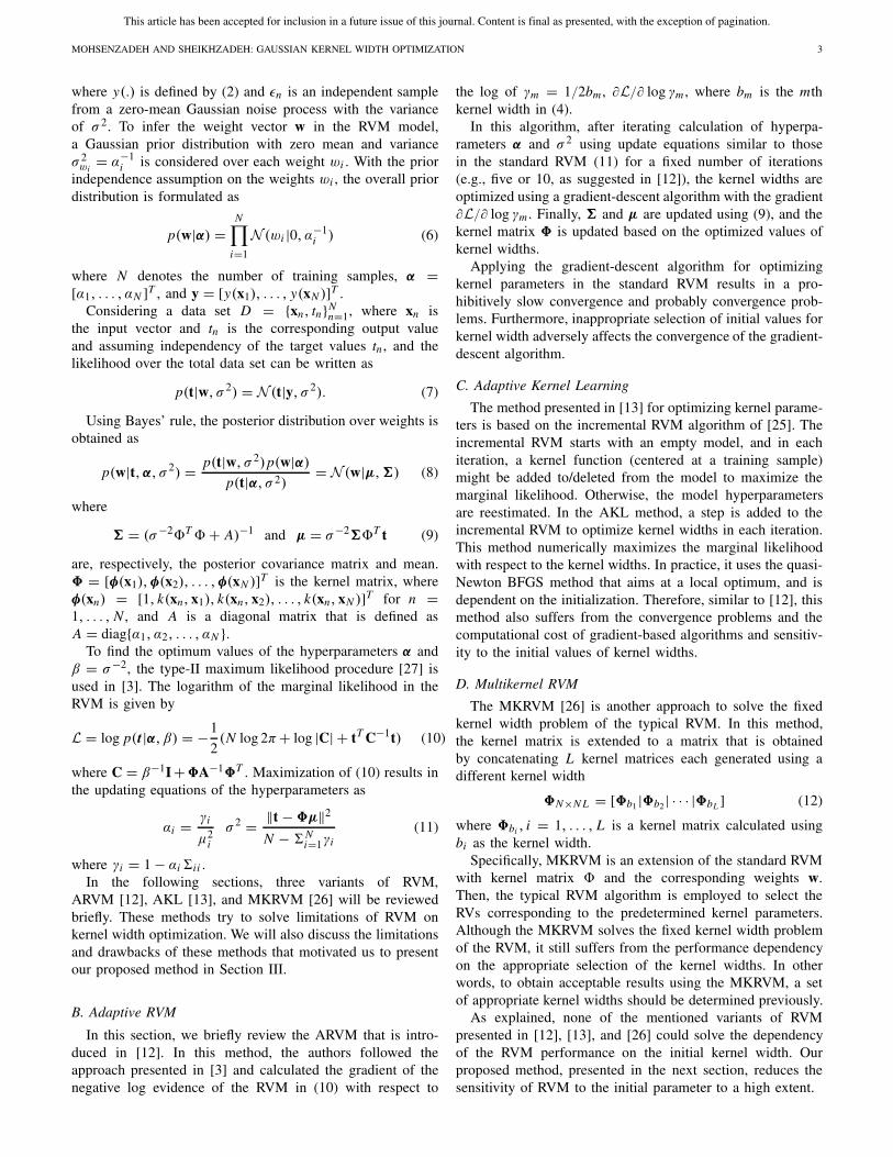
The comparison of marginal likelihood variation in eachiteration for AKORVM (with h = 1) and also RVM (withb = 1) is shown in Fig. 2. As depicted, the marginal likelihoodof the proposed method increases at each iteration, and themaximization with respect to kernel widths can be seen bystepwise improvement in the primary iterations.

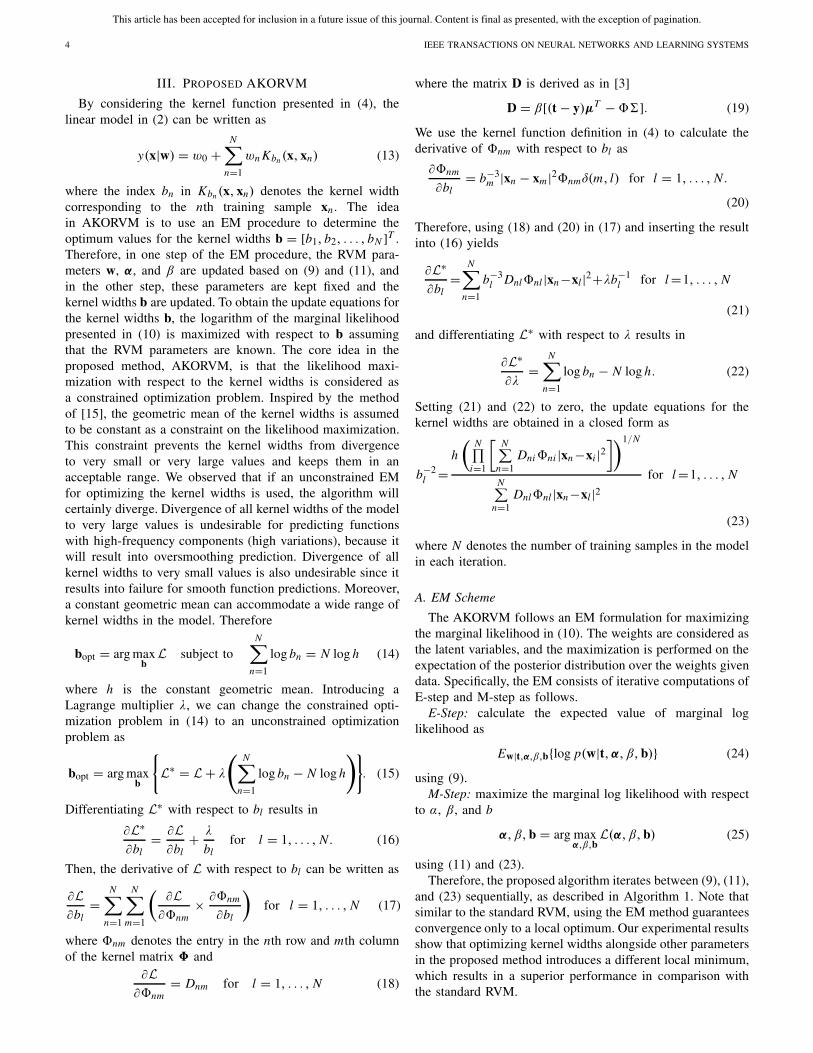
To further investigate the effectiveness of the proposedmethod in reducing the performance sensitivity to the initialvalue of the kernel width, the regression error rate and alsothe number of relevance samples for various kernel widthsare shown in Figs. 3 and 4. The results in these figures areobtained over all 100 samples. Fig. 3 compares the error rateof the proposed method AKORVM and the standard RVM fora wide range of kernel width from 0.1 to 30. The error inthis figure is computed by the root-mean-square formula asRMS= (

∑n(tn − yn)

2/Nt )1/2, where tn ∈ R is the target

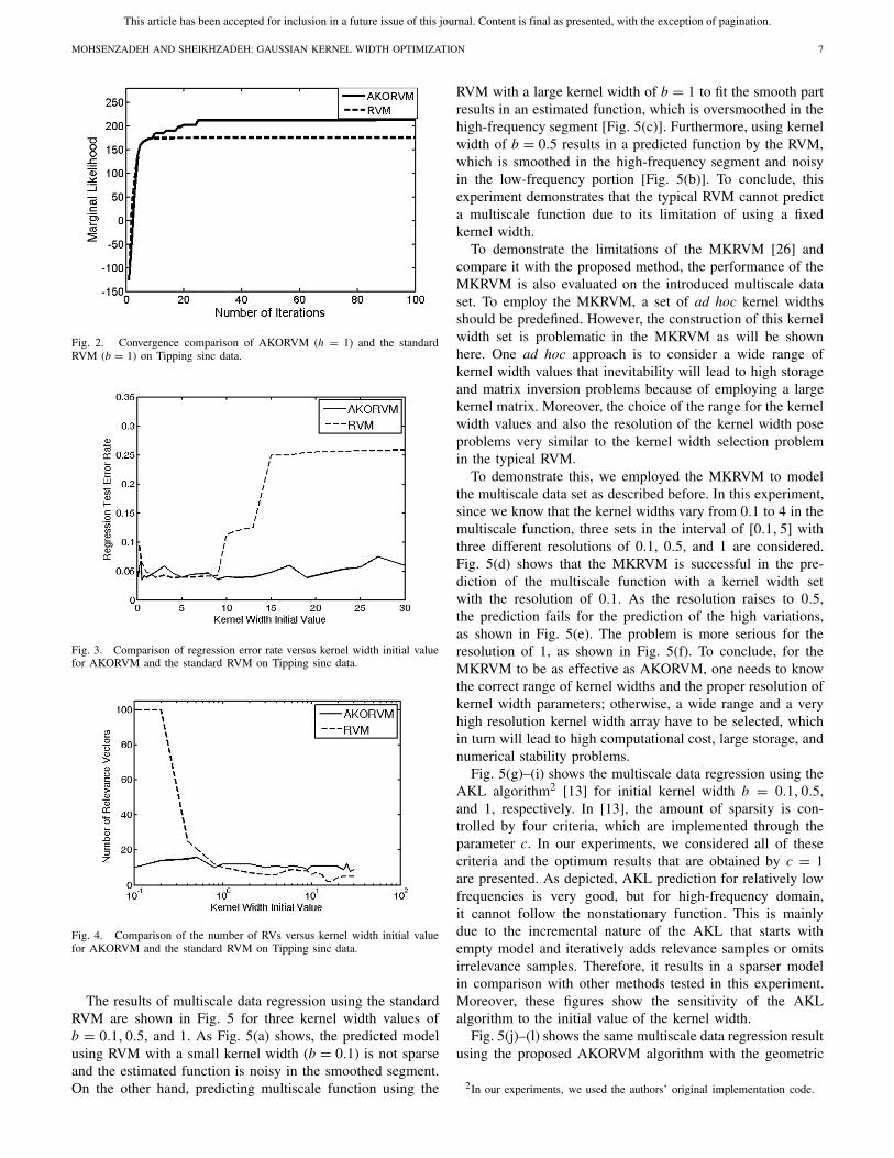
value in the testing set, yn ∈ R is the predicted targetvalue by the regression algorithm, and Nt is the numberof test samples. As depicted, RVM error rate increases forkernel widths of more than eight, while the error rate ofthe AKORVM is almost constant for the whole range ofinitial kernel width (h). Fig. 4 shows the number of RVsin the learned model of RVM and also AKORVM versusdifferent kernel width values. As shown in this figure, thestandard RVM overfits for small kernel widths such that

1In our experiments, we used Tipping’s [3] original implementation of RVM,which is available in http://www.miketipping.com/sparsebayes.htm#software



Fig. 1. Sinc function values versus 100 uniformly spaced samples in the interval [−10, 10]. Sparse Bayesian regression with noisy sinc data: predictedresponse of (a) AKORVM with h = 0.1, (b) RVM with fixed kernel width b = 0.1, (c) AKORVM with h = 4, (d) RVM with fixed kernel width b = 4,(e) AKORVM with h = 30, and (f) RVM with fixed kernel width b = 30.

100 RVs are selected for the learned model. In contrast, theAKORVM learned model contains almost a constant num-ber of relevance samples for a wide range of initial kernelwidths (h). Furthermore, the averaged number of iterationsover all kernel widths tests for the AKORVM is 522.22, whilefor the RVM, it is 514.92. This indicates that the convergencespeed of the proposed method is almost the same as thestandard RVM.

2) Multiscale Data Set: In this section, AKORVM is eval-uated on a multiscale data set to demonstrate its effectiveness

in predicting nonstationary functions in comparison with thestandard RVM [3], MKRVM [26], and also AKL [13]. Themultiscale function

yi = sin(40/xi) + ε for i = 1, . . . , N (26)

is a popular one in [12] and [13]. Following [13], wegenerated N = 128 noisy samples (xi , yi ), where xi isselected uniformly in the interval [1, 10] and ε is drawnfrom a zero-mean Gaussian distribution with the standarddeviation 0.1.



Fig. 2. Convergence comparison of AKORVM (h = 1) and the standardRVM (b = 1) on Tipping sinc data.

Fig. 3. Comparison of regression error rate versus kernel width initial valuefor AKORVM and the standard RVM on Tipping sinc data.

Fig. 4. Comparison of the number of RVs versus kernel width initial valuefor AKORVM and the standard RVM on Tipping sinc data.

The results of multiscale data regression using the standardRVM are shown in Fig. 5 for three kernel width values ofb = 0.1, 0.5, and 1. As Fig. 5(a) shows, the predicted modelusing RVM with a small kernel width (b = 0.1) is not sparseand the estimated function is noisy in the smoothed segment.On the other hand, predicting multiscale function using the

RVM with a large kernel width of b = 1 to fit the smooth partresults in an estimated function, which is oversmoothed in thehigh-frequency segment [Fig. 5(c)]. Furthermore, using kernelwidth of b = 0.5 results in a predicted function by the RVM,which is smoothed in the high-frequency segment and noisyin the low-frequency portion [Fig. 5(b)]. To conclude, thisexperiment demonstrates that the typical RVM cannot predicta multiscale function due to its limitation of using a fixedkernel width.

To demonstrate the limitations of the MKRVM [26] andcompare it with the proposed method, the performance of theMKRVM is also evaluated on the introduced multiscale dataset. To employ the MKRVM, a set of ad hoc kernel widthsshould be predefined. However, the construction of this kernelwidth set is problematic in the MKRVM as will be shownhere. One ad hoc approach is to consider a wide range ofkernel width values that inevitability will lead to high storageand matrix inversion problems because of employing a largekernel matrix. Moreover, the choice of the range for the kernelwidth values and also the resolution of the kernel width poseproblems very similar to the kernel width selection problemin the typical RVM.

To demonstrate this, we employed the MKRVM to modelthe multiscale data set as described before. In this experiment,since we know that the kernel widths vary from 0.1 to 4 in themultiscale function, three sets in the interval of [0.1, 5] withthree different resolutions of 0.1, 0.5, and 1 are considered.Fig. 5(d) shows that the MKRVM is successful in the pre-diction of the multiscale function with a kernel width setwith the resolution of 0.1. As the resolution raises to 0.5,the prediction fails for the prediction of the high variations,as shown in Fig. 5(e). The problem is more serious for theresolution of 1, as shown in Fig. 5(f). To conclude, for theMKRVM to be as effective as AKORVM, one needs to knowthe correct range of kernel widths and the proper resolution ofkernel width parameters; otherwise, a wide range and a veryhigh resolution kernel width array have to be selected, whichin turn will lead to high computational cost, large storage, andnumerical stability problems.

Fig. 5(g)–(i) shows the multiscale data regression using theAKL algorithm2 [13] for initial kernel width b = 0.1, 0.5,and 1, respectively. In [13], the amount of sparsity is con-trolled by four criteria, which are implemented through theparameter c. In our experiments, we considered all of thesecriteria and the optimum results that are obtained by c = 1are presented. As depicted, AKL prediction for relatively lowfrequencies is very good, but for high-frequency domain,it cannot follow the nonstationary function. This is mainlydue to the incremental nature of the AKL that starts withempty model and iteratively adds relevance samples or omitsirrelevance samples. Therefore, it results in a sparser modelin comparison with other methods tested in this experiment.Moreover, these figures show the sensitivity of the AKLalgorithm to the initial value of the kernel width.

Fig. 5(j)–(l) shows the same multiscale data regression resultusing the proposed AKORVM algorithm with the geometric

2In our experiments, we used the authors’ original implementation code.



Fig. 5. Multiscale data regression using standard RVM with kernel width (a) b = 0.1, (b) b = 0.5, and (c) b = 1, MKRVM with resolution (d) 0.1,(e) 0.5, and (f) 1, AKL with initial kernel width (g) b = 0.1, (h) b = 0.5, and (i) b = 1, and AKORVM with the geometric mean of kernel widths (j) h = 0.1,(k) h = 0.5, and (l) h = 1.

Fig. 6. Kernel width values corresponding to the RVs in Fig. 5(l).

mean of kernel widths h = 0.1, 0.5, and 1, respectively. Asdepicted, the AKORVM successfully estimates the nonstation-ary function. The kernel width values corresponding to RVsselected by the AKORVM are shown in Fig. 6 with the sameorder of RVs as those shown in Fig. 5 (by circles). As depicted,

the kernel widths in Fig. 6 vary from very small to relativelylarge values as expected due to multiscale nature of the originalnonstationary function.

In Fig. 5, the four methods RVM, MKRVM, AKL, andAKORVM are compared on the multiscale data set. Eachmethod has its own set of parameters, a fixed kernel width forRVM, a resolution of kernel parameter set for MKRVM, aninitial kernel width for AKL, and finally, a geometric mean ofkernel widths for AKORVM. We chose three identical valuesfor all of these methods to have a fair comparison, and at thesame time, show the limitations of the other three competingmethods.

B. Experiments on Benchmark Data Sets

In this set of experiments, we evaluate the proposed methodAKORVM on five benchmark data sets. In the first experiment,to have a fair comparison, we consider three data sets that have



TABLE I

COMPARISON OF PERFORMANCE (ERROR) AND SPARSITY

(NUMBER OF RVS) ON BENCHMARK DATA SETS

been previously used by our competing methods [12], [13].Following the exact experimental procedure of these compet-ing methods, our results are presented alongside their pub-lished results. Furthermore, in the second set of experiments,the statistical evaluation of the proposed method and alsothe sensitivity of this method to the selection of the singleparameter h (the geometric mean of the kernel widths) areinvestigated on the other two high-dimensional benchmarkdata sets.

1) Comparison With Competing Methods: The proposedmethod is evaluated on three benchmark data sets (Bostonhousing,3 Concrete,4 and Abalone5) to compare its per-formance with those of other existing methods RVM [3],ARVM [12], and AKL [13]. The Boston housing consistsof 506 samples with 13 features, the Concrete contains1030 instances with eight corresponding attributes, and theAblone is a relatively large data set, which contains 4177 sam-ples with eight features. In our experiments, a 10-fold crossvalidation is performed on each data set to estimate the aver-aged generalization error of each method. The error is mea-sured by the mean-square error MSE = ∑Nt

n=1(tn − yn)2/Nt ,

where tn ∈ R is the target value in the testing set, yn ∈ Ris the corresponding target value estimated by the regressionmethod, and Nt is the number of test samples.

Table I depicts the 10-fold cross-validation averaged errorand the averaged number of relevance samples (over 10 folds)for the three benchmark data sets using AKORVM, RVM,ARVM, and AKL. The presented results of the AKL and theARVM in Table I are exactly taken from their reports in [13]and [12]. The results presented in Table I illustrate that themodel sparsity of the AKORVM is comparable with the typicalRVM and the ARVM and inferior to the AKL. This resultis expected because while AKORVM and ARVM employ atop-down approach similar to the standard RVM, the AKL isbased on the fast RVM [25] that uses an incremental approach,and therefore results in a sparser model in comparison withthe standard RVM. As depicted in Table I, the accuracy of

3http://lib.stat.cmu.edu/datasets/boston4http://archive.ics.uci.edu/ml/datasets/Concrete+Compressive+Strength5http://archive.ics.uci.edu/ml/datasets/Abalone

TABLE II

STATISTICAL COMPARISON OF PERFORMANCE (MSE) AND SPARSITY

(NUMBER OF RVS) ON HIGH-DIMENSIONAL BENCHMARK DATA SETS

TABLE III

SENSITIVITY OF PERFORMANCE (MSE) AND SPARSITY

(NUMBER OF RVS) OF THE PROPOSED METHOD TO THE

GEOMETRIC MEAN OF KERNEL WIDTHS ON HIGH-

DIMENSIONAL BENCHMARK DATA SETS

the AKORVM is consistently superior to all the other threemethods of RVM, ARVM, and AKL. Notice that the twomethods ARVM and AKL have a much higher computa-tional complexity compared with our proposed method andthe RVM. Also, in contrast to the AKORVM, the sensitiv-ity of these methods to initial kernel width value selectionis high.

2) Statistical Evaluation and Sensitivity Investigation: Inthis experiment, we investigate the sensitivity of the proposedAKORVM to the geometric mean h on real-world data sets.Two high-dimensional benchmark data sets are consideredfor this experiment. Triazines6 is a high-dimensional data setincluding 186 samples with 61 attributes, and Pyrimidines7 isa relatively high-dimensional data set that contains 74 sampleswith 28 features.

We employed a 10-fold cross-validation procedure on eachdata set to obtain the averaged MSE, averaged number of RVs,and also the standard deviations in each case for a statisticalevaluation of the proposed method. This statistical evaluationsare demonstrated in Table II for AKORVM, RVM, and AKL.In Table II, we reported the best results we obtained for RVMand AKL by employing their original implementation andtuning their parameters.

We also investigated the sensitivity of the proposed methodto the parameter h (geometric mean of kernel widths) on thesetwo data sets. Table III depicts the MSE and also RVs of theproposed method for the optimum geometric mean h and also3h and 1/3 h on each data set. As depicted in Table III, theperformance of the proposed method is not sensitive to the

6http://mldata.org/repository/data/viewslug/regression-datasets-triazines/7http://www4.stat.ncsu.edu/boos/var.select/pyrimidine.html



choice of h for a wide range of this parameter. In contrast,changing the optimal parameters (employed to derive Table II)for the other two methods even on a much smaller scale(less than 50% of the optimal value) would result in rapiddeteriorations.

V. DISCUSSION AND FUTURE WORKS

This paper opts to solve a practical problem in the standardRVM: the performance and the sparsity of the RVM are highlydependent on the choice of appropriate kernel parameters. Inthis paper, we focused on the Gaussian kernel function, whichis a widely used kernel for the typical RVM. However, theproposed method is not limited to the Gaussian kernel. Indeed,the idea can be extended to methods employing other types ofkernel functions (such as exponential kernel, Laplacian kernel,and ANOVA kernel) or even to a mixture of multiple kernelfunctions and also to the multikernel approaches, such as theMKRVM. Leaving out the square of the norm in Gaussiankernel function, the exponential kernel function is obtained as

kexp(xn, xm) = exp

{−‖xn − xm‖

2b2n

}. (27)

The Laplacian kernel function is defined as

kLap(xn, xm) = exp

{−‖xn − xm‖

bn

}. (28)

It can be seen that the Laplacian kernel function is anexponential kernel function, which is less sensitive to the widthparameter. Finally, the ANOVA kernel function is similar toGaussian kernel function, and is well designed for multidi-mensional regression problems [28]. To employ other kernelfunctions with the proposed method, we should calculatethe derivatives of the kernel matrix elements with respect tothe new kernel parameters. Therefore, depending on the newkernel function, (20) should be recalculated, and accordingly,(21) and (23) should be modified. Extending the proposedmethod using the above kernel functions is straightforward.

The proposed method benefits from the fast convergenceof the EM algorithm embedded in the AKORVM algorithm.Using the EM optimization only guarantees convergence to alocal optimum. This is a concern in all EM-based methods,including the standard RVM and AKORVM. In practice, in ourextensive experiments, we did not encounter any problems inusing the EM optimization.

Using the kernel learning approach always raises the risk ofoverfitting to the training data. However, the sparse Bayesianlearning that results in a sparse model prevents overfitting. Thiscan be seen in our extensive experiments on both synthetic andbenchmark data sets in this paper.

Although we presented the kernel width optimization onlyfor regression problems, extending this approach for the sparseBayesian classification tasks is feasible and we will be explor-ing it further as our future work.

VI. CONCLUSION

In this paper, a novel kernel width optimization for the RVMis proposed. Using the training data, the proposed method

simultaneously learns the kernel widths and model parameters.The core idea of the proposed method is to use a constrainedEM-based maximization of marginal likelihood in the RVM.This constraint, which is a fixed geometric mean over thekernel widths, prevents the kernel widths from divergence tovery small or very large values keeping them in an acceptablerange. Using the EM-based optimization results in a veryfast convergence of the proposed method that is superiorto [12] and [13], which use gradient-based algorithms forupdating kernel widths. We evaluated our proposed methodon two synthetic and five real-world benchmark data sets.The evaluation results demonstrate the effectiveness of theproposed method in terms of accuracy and reduction ofperformance sensitivity to the initial kernel width comparingwith the standard RVM and other competing methods.

ACKNOWLEDGMENT

The authors would like to thank D. Tzikas et al. [13], forhelping us by providing their codes.

REFERENCES

[1] C. M. Bishop, Pattern Recognition and Machine Learning. New York,NY, USA: Springer-Verlag, Aug. 2006.

[2] V. N. Vapnik, S. E. Golowi, and A. J. Smola, “Support vector method forfunction approximation, regression estimation and signal processing,”in Proc. 10th Annu. Conf. NIPS, Denver, CO, USA, Dec. 1996,pp. 281–287.

[3] M. Tipping, “Sparse Bayesian learning and the relevance vectormachine,” J. Mach. Learn. Res., vol. 1, pp. 211–244, Jun. 2001.

[4] M. A. Nicolaou, H. Gunes, and M. Pantic, “Output-associative RVMregression for dimensional and continuous emotion prediction,” ImageVis. Comput., vol. 30, no. 3, pp. 186–196, 2012.

[5] A. Thayananthan, R. Navaratnam, B. Stenger, P. H. S. Torr, andR. Cipolla, “Pose estimation and tracking using multivariate regression,”Pattern Recognit. Lett., vol. 29, no. 9, pp. 1302–1310, Jul. 2008.

[6] Q. Duan, J. Zhao, L. Niu, and K. Luo, “Regression based on sparseBayesian learning and the applications in electric systems,” in Proc. 4thICNC, Jinan, China, Oct. 2008, pp. 106–110.

[7] D. Porro, N. Hdez, I. Talavera, O. Nunez, A. Dago, and R. J. Biscay,“Performance evaluation of relevance vector machines as a nonlinearregression method in real-world chemical spectroscopic data,” in Proc.19th ICPR, Tampa, FL, USA, Dec. 2008, pp. 1–4.

[8] S. Wong and R. Cipolla, “Real-time adaptive hand motion recognitionusing a sparse Bayesian classifier,” in Proc. Int. Workshop Comput. Vis.Human-Comput. Interact., Beijing, China, Oct. 2005, pp. 170–179.

[9] A. Agarwal and B. Triggs, “3D human pose from silhouettes byrelevance vector regression,” in Proc. IEEE Comput. Soc. Conf. CVPR,Washington, DC, USA, Jun./Jul. 2004, pp. II-882–II-888.

[10] O. Williams, A. Blake, and R. Cipolla, “Sparse Bayesian learningfor efficient visual tracking,” IEEE Trans. Pattern Anal. Mach. Intell.,vol. 27, no. 8, pp. 1292–1304, Aug. 2005.

[11] Y. Mohsenzadeh, H. Sheikhzadeh, A. M. Reza, N. Bathaee, andM. M. Kalayeh, “The relevance sample-feature machine: A sparseBayesian learning approach to joint feature-sample selection,” IEEETrans. Cybern., vol. 43, no. 6, pp. 2241–2254, Dec. 2013.

[12] J. Yuan, L. Bo, K. Wang, and T. Yu, “Adaptive spherical Gaussian kernelin sparse Bayesian learning framework for nonlinear regression,” ExpertSyst. Appl., vol. 36, no. 2, pp. 3982–3989, Mar. 2009.

[13] D. Tzikas, A. Likas, and N. Galatsanos, “Sparse Bayesian modelingwith adaptive kernel learning,” IEEE Trans. Neural Netw., vol. 20, no. 6,pp. 926–937, Jun. 2009.

[14] S. A. Billings, H. Wei, and M. A. Balikhin, “Generalized multi-scale radial basis function networks,” Neural Netw., vol. 20, no. 10,pp. 1081–1094, 2007.

[15] M. C. Jones and D. A. Henderson, “Maximum likelihood kernel densityestimation: On the potential of convolution sieves,” Comput. Statist. DataAnal., vol. 53, no. 10, pp. 3726–3733, 2009.



[16] M. J. Brewer, “A Bayesian model for local smoothing in kernel densityestimation,” Statist. Comput., vol. 10, no. 4, pp. 299–309, Oct. 2000.

[17] G. Liu, J. Wu, and S. Zhou, “Probabilistic classifiers with a generalizedGaussian scale mixture prior,” Pattern Recognit., vol. 46, no. 1,pp. 332–345, 2013.

[18] M. Filippone, A. F. Marquand, C. R. V. Blain, S. C. R. Williams,J. Mouro-Miranda, and M. Girolami, “Probabilistic prediction of neu-rological disorders with a statistical assessment of neuroimaging datamodalities,” Ann. Appl. Statist., vol. 6, no. 4, pp. 1883–1905, 2012.

[19] J. Quionero-Candela and L. K. Hansen, “Time series prediction basedon the relevance vector machine with adaptive kernels,” in Proc. IEEEICASSP, Orlando, FL, USA, May 2002, pp. 985–988.

[20] R. Hooke and T. A. Leeves, “‘Direct search’ solution of numerical andstatistical problems,” J. ACM, vol. 8, no. 2, pp. 212–229, 1961.

[21] G. R. G. Lanckriet, N. Cristianini, P. Bartlett, L. E. Ghaoui, andM. I. Jordan, “Learning the kernel matrix with semidefiniteprogramming,” J. Mach. Learn. Res., vol. 5, pp. 27–72, Dec. 2004.

[22] M. Girolami and S. Rogers, “Hierarchic Bayesian models for kernellearning,” in Proc. 22nd Int. Conf. Mach. Learn., New York, NY, USA,Aug. 2005, pp. 241–248.

[23] S. Sonnenburg, G. Rtsch, C. Schfer, and B. Schlkopf, “Large scalemultiple kernel learning,” J. Mach. Learn. Res., vol. 7, pp. 1531–1565,Jul. 2006.

[24] B. Krishnapuram, A. J. Hartemink, and M. A. T. Figueiredo,“A Bayesian approach to joint feature selection and classifier design,”IEEE Trans. Pattern Anal. Mach. Intell., vol. 26, no. 9, pp. 1105–1111,Sep. 2004.

[25] M. E. Tipping and A. C. Faul, “Fast marginal likelihood maximizationfor sparse Bayesian models,” in Proc. 9th Int. Workshop Artif. Intell.Statist., Key West, FL, USA, Jan. 2003, pp. 1–13.

[26] M. M. Kalayeh, T. Marin, and J. G. Brankov, “Generalization evaluationof machine learning numerical observers for image quality assessment,”IEEE Trans. Nucl. Sci., vol. 60, no. 3, pp. 1609–1618, Jun. 2013.

[27] J. O. Berger, Statistical Decision Theory and Bayesian Analysis, 2nd ed.New York, NY, USA: Springer-Verlag, 1985.

[28] T. Hofmann, B. Schlkopf, and A. J. Smola, “Kernel methods in machinelearning,” Ann. Statist., vol. 36, no. 3, pp. 1171–1220, 2008.

Yalda Mohsenzadeh received the B.Sc. and M.Sc.degrees in electrical engineering from the FerdowsiUniversity of Mashhad, Mashhad, Iran, and theSharif University of Technology, Tehran, Iran, in2007 and 2009, respectively. She is currently pur-suing the Ph.D. degree in electrical engineeringwith the Multimedia Signal Processing ResearchLaboratory, Department of Electrical Engineering,Amirkabir University of Technology, Tehran.

She is a member of the Multimedia Signal Process-ing Research Laboratory with the Department of

Electrical Engineering, Amirkabir University of Technology. Her currentresearch interests include machine learning, pattern recognition, Bayesianlearning, statistical signal processing, sparse representation, and compressivesensing.

Hamid Sheikhzadeh (M’03–SM’04) received theB.S., M.S., and Ph.D. degrees in electrical engi-neering from the Amirkabir University of Technol-ogy, Tehran, Iran, and the University of Waterloo,Waterloo, ON, Canada, in 1986, 1989, and 1994,respectively.

He was a Faculty Member with the Electrical Engi-neering Department, Amirkabir University of Tech-nology, until 2000, and a Principle Researcher withON Semiconductor, Waterloo, from 2000 to 2008,where he developed signal processing algorithms for

ultralow-power and implantable devices leading to many international patents.He is currently a Faculty Member with the Department of Electrical Engi-neering, Amirkabir University of Technology. His current research interestsinclude signal processing, machine learning, biomedical signal processing, andspeech processing, with particular emphasis on speech recognition, speechenhancement, auditory modeling, adaptive signal processing, subband-basedapproaches, and algorithms for low-power DSP and implantable devices.

gaussian kernel width optimization for sparse bayesian learning

Documents