garch models - lth · garch (generalized arch) i is the most common dynamics variance model. i the...
TRANSCRIPT

GARCH models
Erik Lindström
FMS161/MASM18 Financial Statistics
Erik Lindström GARCH models

Time series models
Let rt be a stochastic process.I µt = E[rt |Ft−1] is the conditional mean modeled by an AR,
ARMA, SETAR, STAR etc. model.I Having a correctly specified model for the conditional mean
allows us to model the conditional variance.I I will for the rest of the lecture assume that rt is the zero
mean returns.I σ2
t = V [rt |Ft−1] is modeled using a dynamic variancemodel.
Erik Lindström GARCH models
Dependence structures
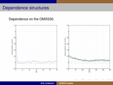
Dependence on the OMXS30.
0 5 10 15 20 25 30−0.2
0
0.2
0.4
0.6
0.8
1
1.2
lag
Au
toco
rre
latio
n, re
turn
s
0 50 100 150 200 250 300−0.2
0
0.2
0.4
0.6
0.8
1
1.2
lag
Au
toco
rre
latio
n, a
bs r
etu
rns
Erik Lindström GARCH models
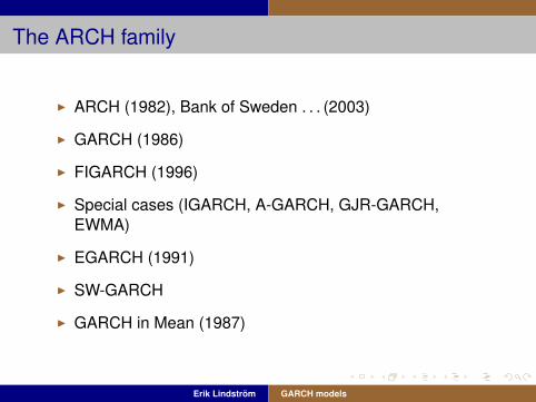
The ARCH family
I ARCH (1982), Bank of Sweden . . . (2003)
I GARCH (1986)
I FIGARCH (1996)
I Special cases (IGARCH, A-GARCH, GJR-GARCH,EWMA)
I EGARCH (1991)
I SW-GARCH
I GARCH in Mean (1987)
Erik Lindström GARCH models
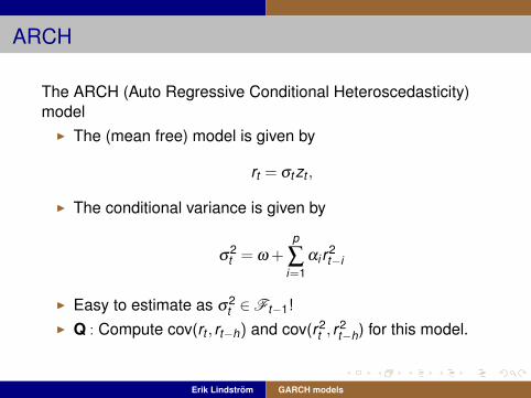
ARCH
The ARCH (Auto Regressive Conditional Heteroscedasticity)model
I The (mean free) model is given by
rt = σtzt ,
I The conditional variance is given by
σ2t = ω +
p
∑i=1
αi r2t−i
I Easy to estimate as σ2t ∈Ft−1!
I Q : Compute cov(rt , rt−h) and cov(r2t , r
2t−h) for this model.
Erik Lindström GARCH models
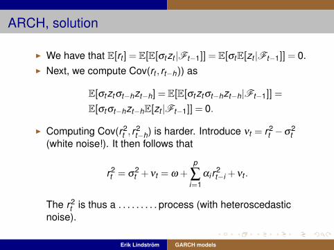
ARCH, solution
I We have that E[rt ] = E[E[σtzt |Ft−1]] = E[σtE[zt |Ft−1]] = 0.I Next, we compute Cov(rt , rt−h)) as
E[σtztσt−hzt−h] = E[E[σtztσt−hzt−h|Ft−1]] =
E[σtσt−hzt−hE[zt |Ft−1]] = 0.
I Computing Cov(r2t , r
2t−h) is harder. Introduce νt = r2
t −σ2t
(white noise!). It then follows that
r2t = σ
2t + νt = ω +
p
∑i=1
αi r2t−i + νt .
The r2t is thus a . . . . . . . . . process (with heteroscedastic
noise).
Erik Lindström GARCH models

ARCH, limitations
I Large number of lags are needed to fit data.I The model is rather restrictive, as the parameters must be
bounded if moments should be finiteI (Exercise: Compute the restrictions for the ARCH(1) model
to have finite variance and kurtosis.)
Erik Lindström GARCH models

GARCH (Generalized ARCH)
I Is the most common dynamics variance model.I The conditional variance is given by
σ2t = ω +
p
∑i=1
αi r2t−i +
q
∑j=1
βjσ2t−j
I A GARCH(1,1) is often sufficent!I Conditions on the parameters.
Erik Lindström GARCH models
GARCH
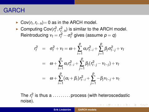
I Cov(rt , rt−h)= 0 as in the ARCH model.I Computing Cov(r2
t , r2t−h) is similar to the ARCH model.
Reintroducing νt = r2t −σ2
t gives (assume p = q)
r2t = σ
2t + νt = ω +
p
∑i=1
αi r2t−i +
p
∑j=1
βjσ2t−j + νt
= ω +p
∑i=1
αi r2t−i +
p
∑j=1
βj(r2t−j −νt−j) + νt
= ω +p
∑i=1
(αi + βi)r2t−i +
p
∑j=1−βjνt−j + νt
The r2t is thus a . . . . . . . . . process (with heteroscedastic
noise).
Erik Lindström GARCH models

Estimation of GARCH(1,1) on OMXS30 logreturns
ω = 1.9 ·10−6, α1 = 0.0775 β1 = 0.9152
2000 2010
−0.05
0
0.05
0.1
OMXS30 logreturns
2000 2010
0.01
0.015
0.02
0.025
0.03
0.035
0.04
Extimated GARCH(1,1) vol
2000 2010
−4
−2
0
2
4
OMXS30 normalised logreturns
−4 −2 0 2 4
0.0010.0030.01 0.02 0.05 0.10 0.25 0.50 0.75 0.90 0.95 0.98 0.99
0.9970.999
Data
Pro
ba
bili
ty
NORMPLOT OMXS30 normalised logreturns
Erik Lindström GARCH models
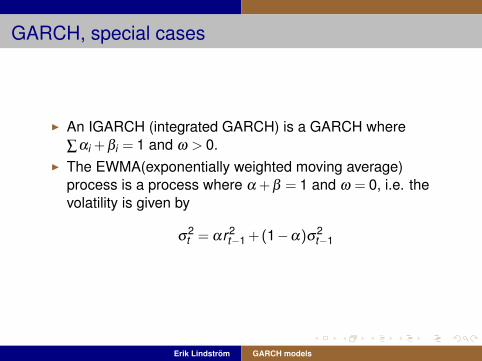
GARCH, special cases
I An IGARCH (integrated GARCH) is a GARCH where∑αi + βi = 1 and ω > 0.
I The EWMA(exponentially weighted moving average)process is a process where α + β = 1 and ω = 0, i.e. thevolatility is given by
σ2t = αr2
t−1 + (1−α)σ2t−1
Erik Lindström GARCH models
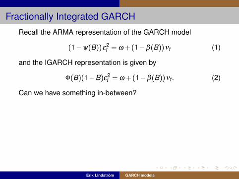
Fractionally Integrated GARCH
Recall the ARMA representation of the GARCH model
(1−ψ(B))ε2t = ω + (1−β (B))νt (1)
and the IGARCH representation is given by
Φ(B)(1−B)ε2t = ω + (1−β (B))νt . (2)
Can we have something in-between?
Yes, that is the FIGARCHmodel
Φ(B)(1−B)dε
2t = ω + (1−β (B))νt (3)
with the process having finite variance if −.5 < d < 0.5. Thefractional differentiation can be computed as
(1−B)d =∞
∑k=0
Γ(k −d)
Γ(k + 1)Γ(−d)Bk . (4)
Erik Lindström GARCH models
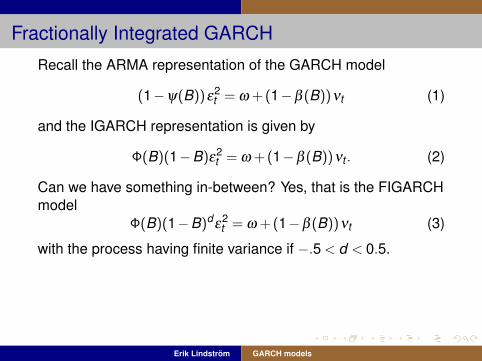
Fractionally Integrated GARCH
Recall the ARMA representation of the GARCH model
(1−ψ(B))ε2t = ω + (1−β (B))νt (1)
and the IGARCH representation is given by
Φ(B)(1−B)ε2t = ω + (1−β (B))νt . (2)
Can we have something in-between? Yes, that is the FIGARCHmodel
Φ(B)(1−B)dε
2t = ω + (1−β (B))νt (3)
with the process having finite variance if −.5 < d < 0.5.
Thefractional differentiation can be computed as
(1−B)d =∞
∑k=0
Γ(k −d)
Γ(k + 1)Γ(−d)Bk . (4)
Erik Lindström GARCH models

Fractionally Integrated GARCH
Recall the ARMA representation of the GARCH model
(1−ψ(B))ε2t = ω + (1−β (B))νt (1)
and the IGARCH representation is given by
Φ(B)(1−B)ε2t = ω + (1−β (B))νt . (2)
Can we have something in-between? Yes, that is the FIGARCHmodel
Φ(B)(1−B)dε
2t = ω + (1−β (B))νt (3)
with the process having finite variance if −.5 < d < 0.5. Thefractional differentiation can be computed as
(1−B)d =∞
∑k=0
Γ(k −d)
Γ(k + 1)Γ(−d)Bk . (4)
Erik Lindström GARCH models

EGARCH (Exponential GARCH)
I The conditional variance is given by
logσ2t = ω +
p
∑i=1
αi f (rt−i) +q
∑j=1
βj logσ2t−j
I logσ2 may be negative!I Thus no (fewer) restrictions on the parameters.
Erik Lindström GARCH models
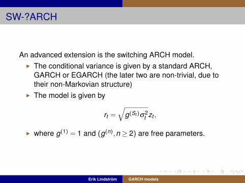
SW-?ARCH
An advanced extension is the switching ARCH model.I The conditional variance is given by a standard ARCH,
GARCH or EGARCH (the later two are non-trivial, due totheir non-Markovian structure)
I The model is given by
rt =√
g(St )σ2t zt ,
I where g(1) = 1 and (g(n),n ≥ 2) are free parameters.
Erik Lindström GARCH models
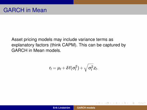
GARCH in Mean
Asset pricing models may include variance terms asexplanatory factors (think CAPM). This can be captured byGARCH in Mean models.
rt = µt + δ f (σ2t ) +
√σ2
t zt .
Erik Lindström GARCH models

Variations
Several improvements can be applied to any of the models.I Bad news tend to increase the variance more than good
news. We can replace r2t−i by
I (rt−i + γ)2 (Type I)I (|rt−i |+ cr2
t−i ) (Type II)I Replace αi with (αi + α̃i1{rt−i<0})
(GJR, Glosten-Jagannathan-Runkle).I DistributionsI Stationarity problems.
Erik Lindström GARCH models

Multivariate models
What about multivariate models?I Huge number of models.
I VEC-MVGARCH (1988)I BEKK-MVGARCH (1995)I CCC-MVGARCH (1990)I DCC-MVGARCH (2002)I STCC-MVGARCH(2005)
I Most are overparametrized.I I recommend starting with the CCC-MVGARCHI Returns: Rt = H1/2
t ZtI Ht = ∆tPc∆t where
I ∆ = diag(σt ,k )I Pc is a constant correlation matrix.
Erik Lindström GARCH models
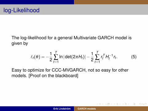
log-Likelihood
The log-likelihood for a general Multivariate GARCH model isgiven by
`t (θ) =−12
T
∑t=1
ln |det(2πHt )|−12
T
∑t=1
rTt H−1
t rt . (5)
Easy to optimize for CCC-MVGARCH, not so easy for othermodels. [Proof on the blackboard]
Erik Lindström GARCH models

Some wellknown Swedish assets
On the second computer exercise you will try to fit aCCC-MVGARCH model to this.
2005 2006 2007 2008 2009 20100
100
200
300
400
500
600
ABBAstrazeneca
B
BolidenInvestor
B
LundinMTG
B
NordeaTele2
B
Erik Lindström GARCH models