games, graphs, and geometry
TRANSCRIPT

GAMES, GRAPHS, AND GEOMETRY
BY WESLEY PEGDEN
A dissertation submitted to the
Graduate School—New Brunswick
Rutgers, The State University of New Jersey
in partial fulfillment of the requirements
for the degree of
Doctor of Philosophy
Graduate Program in Mathematics
Written under the direction of
Jozsef Beck
and approved by
New Brunswick, New Jersey
May, 2010

ABSTRACT OF THE DISSERTATION
Games, Graphs, and Geometry
by Wesley Pegden
Dissertation Director: Jozsef Beck
This thesis concerns four separate topics: the balanced counterpart of the Hales-Jewett
number, the maximal density of k-critical triangle-free graphs, Euclidean sets resilient
to an ‘erosion’ operation, and an extension of the Local Lemma which can be applied
in a game setting.
For the Hales-Jewett number, our motivation comes from a desire to show that there
are infinitely many ‘delicate’ Tic-Tac-Toe games. Roughly speaking, these are games
where neither player has a simple reason for having a winning/drawing strategy. The
first part of this thesis concerns the translation of bounds on the famous ‘Hales-Jewett
number’ into bounds on the ‘Halving Hales-Jewett number’, its ‘balanced’ version,
which give the desired game-theoretic consequences.
The second part of this thesis concerns k-critical triangle-free graphs: can they
have quadratic edge-density, independent of k as k grows large? This question has
close connections both to the study of the density of critical graphs, and the study of
the chromatic number of triangle-free graphs. Surprisingly, we are able to determine
the exact asymptotic density of k-critical triangle-free graphs for k ≥ 6, and even for
pentagon-and-triangle-free graphs.
In the third part, we will consider a simple erosion operation on sets in Euclidean
space, which roughly represents the operation of ‘shaving off’ points near the boundary
ii

of a set. We will give a complete characterization of sets whose shape is unchanged by
this operation.
Finally, in the fourth part, we will generalize the classical Lovasz Local Lemma to
a ‘Lefthanded’ version, which, roughly speaking, allows one to ignore dependencies ‘to
the right’ when making an application of the Local Lemma to bad events which have
an underlying order. This will allow us to prove game-theoretic analogs of classical
results on nonrepetitive sequences, representing the first successful applications of a
Local Lemma to games.
iii

Acknowledgements
I would like to thank Andras Gyarfas for helpful discussions and encouragement on
the problem considered in Chapter 3 (and in particular, for giving the construction
illustrated in Figure 3.3). For Chapter 5, thanks are due for helpful conversations with
Jaroslaw Grytczuk regarding nonrepetitive sequences. I would also like to thank Jeff
Kahn, Joel Spencer, and Doron Zeilberger for their service on my committee, and Mike
Saks for discussions and advice in his role as director of the Graduate Program. Finally,
I thank my advisor, Jozsef Beck, for his constant and enthusiastic encouragement and
support, and for many, many discussions on all the problems considered in this thesis.
iv

Table of Contents
Abstract . . . . . . . . . . . . . . . . . . . . . . . . . . . . . . . . . . . . . . . . ii
Acknowledgements . . . . . . . . . . . . . . . . . . . . . . . . . . . . . . . . . iv
1. Introduction . . . . . . . . . . . . . . . . . . . . . . . . . . . . . . . . . . . 1
2. Tic-Tac-Toe and the halving Hales-Jewett number . . . . . . . . . . . 12
2.1. Which Halving Hales-Jewett number? . . . . . . . . . . . . . . . . . . . 14
2.2. Proving HJ 12(n) ≥ HJ(n− 2) . . . . . . . . . . . . . . . . . . . . . . . . 15
2.3. Further questions . . . . . . . . . . . . . . . . . . . . . . . . . . . . . . . 19
3. Odd-girth in dense k-critical graphs . . . . . . . . . . . . . . . . . . . . 21
3.1. Avoiding triangles (constructions) . . . . . . . . . . . . . . . . . . . . . 23
3.1.1. Constructing Gk . . . . . . . . . . . . . . . . . . . . . . . . . . . 27
3.1.2. Density of Gk (for k ≥ 6) . . . . . . . . . . . . . . . . . . . . . . 28
3.1.3. Density of G5 . . . . . . . . . . . . . . . . . . . . . . . . . . . . . 29
3.2. Avoiding pentagons (existence result) . . . . . . . . . . . . . . . . . . . 30
3.3. Avoiding more odd cycles (ℓ ≥ 7) for k = 4 . . . . . . . . . . . . . . . . 34
3.4. Further Questions . . . . . . . . . . . . . . . . . . . . . . . . . . . . . . 35
4. Sets resilient to erosion . . . . . . . . . . . . . . . . . . . . . . . . . . . . 39
4.1. The bounded case . . . . . . . . . . . . . . . . . . . . . . . . . . . . . . 42
4.2. The general convex case . . . . . . . . . . . . . . . . . . . . . . . . . . . 49
4.2.1. Unbounded convex examples in R3 . . . . . . . . . . . . . . . . . 50
4.2.2. Characterizing all resilient convex bodies in Rn . . . . . . . . . . 51
4.2.3. Convex sets resilient to expansion . . . . . . . . . . . . . . . . . 55
4.3. The nonconvex case . . . . . . . . . . . . . . . . . . . . . . . . . . . . . 56
v

4.3.1. Characterizing nonconvex resilient sets . . . . . . . . . . . . . . . 58
4.3.2. Fractals and erosion . . . . . . . . . . . . . . . . . . . . . . . . . 62
4.4. Further Questions . . . . . . . . . . . . . . . . . . . . . . . . . . . . . . 64
5. Winning strategies from a Lefthanded Local Lemma . . . . . . . . . . 67
5.1. An easier game . . . . . . . . . . . . . . . . . . . . . . . . . . . . . . . . 72
5.2. Lefthanded Local Lemma . . . . . . . . . . . . . . . . . . . . . . . . . . 76
5.3. Thue-type binary sequence games . . . . . . . . . . . . . . . . . . . . . . 79
5.3.1. Long identical intervals can be made far apart . . . . . . . . . . 79
5.3.2. Adjacent intervals can be made very different . . . . . . . . . . . 81
5.4. c-ary nonrepetitive sequence games . . . . . . . . . . . . . . . . . . . . . 83
5.5. Pattern avoidance . . . . . . . . . . . . . . . . . . . . . . . . . . . . . . 90
5.6. Further Questions . . . . . . . . . . . . . . . . . . . . . . . . . . . . . . 92
References . . . . . . . . . . . . . . . . . . . . . . . . . . . . . . . . . . . . . . . 97
Vita . . . . . . . . . . . . . . . . . . . . . . . . . . . . . . . . . . . . . . . . . . . 101
vi

1
Chapter 1
Introduction
Discrete Mathematics is a young branch of Mathematics in all important senses. Its
grand classical problems (the 4-coloring theorem, for example, or the perfect graph
conjectures) have been solved in recent memory, rather than in the distant past, while
defining problems with no solution in sight (such as the P=NP? problem) are decades
rather than centuries old. At the same time, completely new and surprising directions of
inquiry are constantly being discovered, as is the case, for example, with the relatively
recent attention focused on combinatorial games, or the rise of additive combinatorics
as a major focus of attention. Discrete mathematics is a discipline which shows no
shortage of new directions; no shortage of new mysteries to be uncovered.
In a reflection of the varied richness of the field, this thesis is not confined to the ex-
amination of a single problem, but instead concerns several problems we have addressed;
the only common thread is the pursuit of nice questions. We will use new results about
the classical Hales-Jewett number to show the existence of infinitely many ‘delicate’
Tic-Tac-Toe games, achieve uncharacteristically optimal results through a new inquiry
in the classical area of color-critical graphs, prove a surprising characterization of Eu-
clidean sets ‘resilient’ to ‘erosion’, and develop a generalization of the Lovasz Local
Lemma which allows a new kind of probabilistic approach to certain combinatorial
games.
* * *
Motivation for the study of the Hales-Jewett number comes from nd Tic-Tac-Toe games,
higher-dimensional analogs of the 32 (or 3× 3) game played by children. The classical
Hales-Jewett number HJ(n) can be defined as the smallest dimension D for which it is
impossible to mark the cells of the nD hypercube with x’s and o’s in such a way that

2
there are no ‘n-in-a-line’ Tic-Tac-Toe winning sets which are either all x’s or all o’s.
This immediately implies, then, that whenever d ≥ HJ(n), a Tic-Tac-Toe game on the
nd board cannot end in a draw. The simple-yet-powerful strategy stealing argument
implies that Player 2 can never win a Tic-Tac-Toe game when Player 1 is playing
perfectly, and so Player 1 has a winning strategy at Tic-Tac-Toe on the nd board when
d ≥ HJ(n)—for these games, the Ramsey-theoretic Hales-Jewett number is enough to
deduce the existence of a winning strategy for Player 1. To this day, upper bounds
on the Hales-Jewett number are the only results which prove the existence of winning
strategies for large Tic-Tac-Toe games.
Nevertheless, it is perhaps worth noticing that Tic-Tac-Toe games where d ≥ HJ(n)
are a bit strange from the standpoint of competitive play. After all, these are games
where a draw is impossible, and the players are simply competing to be the first to get
n-in-a-line. This kind of ‘winning by Ramsey theory’ seems quite different from the
behavior of more familiar Tic-Tac-Toe games. The 43 Tic-Tac-Toe game (Qubic) was
played competitively, and was shown by Patashnik’s huge computer-assisted work [44]
to be a first player win, but this is a game where drawing positions are plentiful: Player
1 wins because he is able to skillfully avoid them. This is what is called a ‘delicate win’
for Player 1—he can win the game even though a draw is possible.
Normally, ‘winning’ in Tic-Tac-Toe means getting n-in-a-line before the other player.
It turns out that this is much harder than trying to get n-in-a-line if you are willing to let
your opponent beat you to it. Although anyone who has played it knows that ordinary
3× 3 Tic-Tac-Toe ends in a draw so long as Player 2 makes no mistakes, it is actually
easy for Player 1 to get 3 x’s in a row in this game—he just may have to let Player 2
get 3 o’s in a row first. This alternative goal corresponds to what is called a ‘weak win’
in a positional game, where Player 1 achieves his goal, although not necessarily before
Player 2. The ‘fake probabilistic theory’ developed by Beck allows analysis of ‘weak
wins’ for positional games, and in particular, has succeeded at determining the behavior
of the ‘weak win’ with respect to the dimension for Tic-Tac-Toe (in stark contrast to
the lack of knowledge about the growth of the Hales-Jewett number, for example). In
particular, Beck has shown [5] that Player 1 has a strategy for a ‘weak win’ in the nd

3
Tic-Tac-Toe game if d > log 22 n2, while, on the other hand, Player 2 can prevent Player
1 from even achieving a weak win if d < ( log 216 − o(1)) n2
logn . When Player 2 can prevent
Player 1 from achieving a weak win, we say he has a ‘strong draw’. In cases like the
familiar 3 × 3 Tic-Tac-Toe game where this is not the case we say that Player 2 has
a ‘delicate draw’. Such cases present what are perhaps the most interesting drawing
strategies for Player 2, since they depend on Player 2’s ability to create his own threats
to prevent Player 1 from winning.
It is natural to wonder how many Tic-Tac-Toe games fall into the classes of ‘delicate
win’ and ‘delicate draw’ described above, since these seem to be the most interesting
classes of Tic-Tac-Toe games, in some sense (and, certainly, the most difficult classes
to analyze mathematically). Unfortunately, other than the 32 and 43 games already
mentioned, no other examples of ‘delicate’ Tic-Tac-Toe games are known at all. And
it is unknown, for example, whether either class could consist of just the single game
already known in it.
On the other hand, through recent work with Beck and Vijay, we have shown that
the union of these two classes must contain infinitely many Tic-Tac-Toe games. In
particular, our joint paper [7] contains a new exponential lower bound HJ(n) ≥ 2n/4
3n4 on
the Hales-Jewett number HJ(n), improving the previous best-known bound HJ(n) ≥ n
from the original paper of Hales and Jewett. This almost implies that there are terminal
drawing positions in nd Tic-Tac-Toe games when d < 2n/4
3n4 , but not quite, since the
colorings guaranteed to exist for this result are not necessarily ‘balanced’ colorings
(the number of x’s and o’s may differ by more than one). The quantity we would like
to bound for implications to Tic-Tac-Toe is the halving Hales-Jewett number HJ 12(n),
defined as the minimum d0 for which any balanced coloring of nd results in an all-x’s
or all-o’s n-a-line when d ≥ d0. Coupled with Beck’s results on the weak-win, a super-
quadratic bound on HJ 12(n) would imply that there are infinitely many Tic-Tac-Toe
games where d is large enough relative to n that Player 2 doesn’t have a strong draw,
but where d is small enough relative to n that Player 1 doesn’t have a strong win either.

4
In Chapter 2 we will present a proof (also in [7]) that
HJ 12(n) ≥ HJ(n− 2),
implying an exponential lower bound for HJ 12(n) from the already mentioned bound
for HJ(n), and implying the existence of infinitely many ‘delicate’ Tic-Tac-Toe games.
* * *
There is a recurring theme in graph theory concerning the comparison of bipartite
graphs with triangle-free graphs, since the former are graphs without any odd cycles,
and the latter are graphs avoiding just the shortest kind of odd cycles. To what extent
does avoiding triangles force these families behave similarly? It is an old result that
triangle-free graphs can have arbitrarily large chromatic number, but the classical con-
structions to demonstrate this (due to Zykov [56] and Mycielski [40], for example) are
strikingly sparse graphs. This suggests that perhaps triangle-free graphs have trouble
distinguishing themselves from bipartite graphs when they are required to have lots of
edges (a suggestion further encouraged by the fact that a triangle-free graph with the
maximum possible number of edges is a complete bipartite graph).
We need to be careful what kind of questions we ask, however. In fact, it is easy to
see that there are triangle-free graphs of large chromatic number and with a quadratic
number of edges, since we can take the disjoint union of a k-chromatic triangle-free
graph with a large complete bipartite graph. These kinds of considerations motivated
Erdos and Simonovits to ask about the minimum degree of triangle-free graphs with
large chromatic number, an issue which has recently been essentially resolved [11].
One can use the concept of k-criticality to ask another kind of question about dense
triangle-free graphs. A graph is k-critical if it is k-chromatic and removing any edge
results in a (k − 1)-critical graph, thus it is clear that if we create dense triangle-
free graph by taking disjoint unions with bipartite graphs, the results will be far from
critical. This motivates the question: does there exist a family of triangle-free
critical graphs of arbitrarily large chromatic number, and each with > cn2

5
edges for some fixed c > 0?1
In Chapter 3 we will answer this question in the affirmative, by proving the following
theorem:
Theorem 1.1. For k ≥ 4, there are triangle-free k-critical graphs with > (ck− o(1))n2
edges, where here c4 ≥ 116 , c5 ≥ 4
31 , and ck = 14 for all k ≥ 6.
Apart from the connection to the study of triangle-free graphs, this issue is closely
related to the study of the density of critical graphs, which began with a question of
Erdos, leading to the construction by Dirac of k-critical graphs (k ≥ 6) with > 14n
2
edges. Toft subsequently constructed a 4-critical graph with > 116n
2 edges; curiously,
Toft’s graph is triangle-free. Applying Mycielski’s operation to Toft’s graph is a simple
way to get k-critical triangle-free graphs with 116(34)k−4n2 edges; thus, the graphs have
quadratic density for each k—this does not answer the question we are interested in,
however, since the density constant 116(34)k−4 tends to 0 as k grows large.
Theorem 1.1, on the other hand, implies that quadratic density can in fact be
maintained as k grows large, since the constant ck does not tend to 0 as k goes to
infinity. Apart from that, the constant ck = 14 given in Theorem 1.1 for the case k ≥ 6
is even best possible, since Turan’s theorem implies that triangle-free graphs have ≤ 14n
2
edges.
In this sense, Theorem 1.1 stands out as an exception in the study of critical graphs
to the rule that optimal results are not generally attainable. The problem is that
there are no good techniques known to prove upper bound results for the density of
critical graphs—in fact, it may be that essentially all known upper bound results for
the density of critical graphs come from applications of Turan’s theorem. (Observe,
for example, that a k-critical graph with more thank2
edges cannot contain Kk as a
subgraph.) With Theorem 1.1, we are simply lucky that the lower bounds we achieve
line up with the trivial Turan theorem upper bound. Chapter 3 also contains the proof
of the following theorem with the same striking feature:
1This question is quite similar to problems discussed by Erdos in [22], but this particular formulationappears to have been ignored—all the more suprising since it gives rise to optimum results.

6
not resilient resilient
Figure 1.1: Some erosions of bounded shapes in R2. The area in gray is what is removedby an erosion operation.
Theorem 1.2. For k ≥ 4, there are pentagon-and-triangle-free k-critical graphs with
> (c5,k − o(1))n2 edges, where c5,4 ≥ 136 , c5,5 ≥ 3
35 , and c5,k = 14 for k ≥ 6.
It seems, in fact, that these two theorems give us the only natural familes of graphs
(triangle-free and pentagon-and-triangle-free graphs, respectively) where the asymp-
totic density of critical members are known. Finally, in Chapter 1.1 we will also present
the following result for 4-critical graphs of larger odd-girth:
Theorem 1.3. For each odd ℓ, there are 4-critical graphs without odd cycles of length
≤ ℓ with > ( 1ℓ+1)2n2 edges.
* * *
Consider a subset X of Euclidean space. We can define a simple ‘erosion’ operation
er(X) = X \ y∈XC B(r, y) which removes from X any points at distance < r of the
complement of X. (B(r, y) denotes an open ball of radius r about a point y.) The
effect of this operation on some familiar shapes is shown in Figure 1.1. This operation
is natural enough that it has been studied from a practical standpoint, as a model of
pebble erosion (see, e.g., [20]). However, there is a quite natural theoretical question
which is immediately suggested by the operation—for which sets (and radii) does
the erosion operation produce a set which is equivalent to the original under
a Euclidean similarity transformation? When X is similar to er(X), X is said to
be resilient to erosion by the radius r.
Referring again to Figure 1.1, it is clear that a closed disk is resilient to erosion,
as are, for example, the closed bodies of regular polygons. Bodies of triangles are also
resilient: when their erosion consists of more than just a single point, it is the body
of another triangle with the same angles, and so is similar to the original set. The
body of an irregular rectangle, on the other hand, is not resilient, since the ratio of

7
(a) A portion of an unbounded (and scale-invariant) version of Koch’s curve.
(b) Part of an unbounded resilient set derived from the unbounded version of Koch’ssnowflake. The area removed by two successive erosion operations is shown in twodifferent shades of gray. Note that erosion makes it ‘bigger’.
Figure 1.2: Getting a resilient set from the Koch curve.
the side-lengths changes upon erosion—and of course, it should be clear that ‘typical’
shapes will not be resilient to erosion by any positive radius. In Chapter 4, we will
prove the following characterization of bounded resilient sets:
Theorem 1.4. A bounded set X ⊂ Rn is resilient to erosion by some radius r > 0 if
and only if it is a closed convex set with an inscribed ball of radius > r.
The definition of an ‘inscribed ball’ will be given in Chapter 4, but for now, we
will point out that it is not a coincidence that all the resilient polygons from Figure
1.1 have inscribed circles. Although Theorem 1.4 provides a complete and elegant
characterization of bounded resilient sets, it requires a surprisingly technical proof when
the dimension n is greater than 2, due to annoying possibilities which must be allowed
for—for example, that the set X is resilient to erosion, with corresponding similarity
transformations which always include irrational rotations.
We will see in Chapter 4 that it is possible to extend Theorem 1.4 to a result which
covers unbounded convex sets. It might seem reasonable, perhaps, to expect that all
resilient sets are convex, so that this would constitute a complete characterization of
resilient subsets of Eucliean space. This, it turns out, is not even close to being true,

8
Figure 1.3: A cropped example of a fractal-like unbounded resilient set from R2. Thegray area is the region removed from the set upon an erosion by the smallest radiusby which it is erosion-resilient. The corresponding similarity transformation is thehomothety which fixes the center of the region shown and increasing distances by afactor of 7.
9
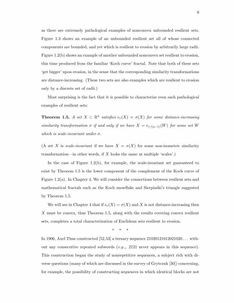
as there are extremely pathological examples of nonconvex unbounded resilient sets.
Figure 1.3 shows an example of an unbounded resilient set all of whose connected
components are bounded, and yet which is resilient to erosion by arbitrarily large radii.
Figure 1.2(b) shows an example of another unbounded nonconvex set resilient to erosion,
this time produced from the familiar ‘Koch curve’ fractal. Note that both of these sets
‘get bigger’ upon erosion, in the sense that the corresponding similarity transformations
are distance-increasing. (These two sets are also examples which are resilient to erosion
only by a discrete set of radii.)
Most surprising is the fact that it is possible to characterize even such pathological
examples of resilient sets:
Theorem 1.5. A set X ⊂ Rn satisfies er(X) = σ(X) for some distance-increasing
similarity transformation σ if and only if we have X = er/(α−1)(W ) for some set W
which is scale-invariant under σ.
(A set X is scale-invariant if we have X = σ(X) for some non-isometric similarity
transformation—in other words, if X looks the same at multiple ‘scales’.)
In the case of Figure 1.2(b), for example, the scale-invariant set guaranteed to
exist by Theorem 1.5 is the lower component of the complement of the Koch curve of
Figure 1.2(a). In Chapter 4, We will consider the connections between resilient sets and
mathematical fractals such as the Koch snowflake and Sierpinski’s triangle suggested
by Theorem 1.5.
We will see in Chapter 4 that if er(X) = σ(X) and X is not distance-increasing then
X must be convex, thus Theorem 1.5, along with the results covering convex resilient
sets, completes a total characterization of Euclidean sets resilient to erosion.
* * *
In 1906, Axel Thue constructed [52,53] a ternary sequence 21020121012021020 . . . with-
out any consecutive repeated subwords (e.g.,, 2121 never appears in this sequence).
This construction began the study of nonrepetitive sequences, a subject rich with di-
verse questions (many of which are discussed in the survey of Grytczuk [30]) concerning,
for example, the possibility of constructing sequences in which identical blocks are not

10
only nonadjacent but far apart.
Any question about nonrepetitive sequences has a natural ‘game’ analog: suppose
Players 1 and 2 take turns choosing digits of an unending c-ary sequence (Player 1
chooses the first digit from the set {1, 2, . . . , c}, Player 2 chooses the second digit from
the same set, Player 1 chooses the third digit, and so on). What kind of nonrepeti-
tiveness can Player 1 achieve in this game? Of course, through imitation, Player 2 can
make repetitions of single digits. It turns out, however, that when c is sufficiently large
and Player 1 is playing well, that is the best Player 2 can hope to achieve:
Theorem 1.6. Player 1 has a strategy in the 37-ary sequence game which ensures that
there will be no identical adjacent blocks of length ≥ 2.
Theorem 1.6 thus gives a natural game-theoretic analog to Thue’s old theorem on
nonrepetitive sequences.
The biggest surprise regarding Theorem 1.6 is that it is proved with a Local Lemma.
Previous attempts to apply the Local Lemma to games have failed, as the unknown
second player’s strategy typically introduces a mess of dependencies which removes any
possibility of demonstrating the kind of “only local dependence” criterion needed to
apply the Local Lemma. (In a nutshell, how can we argue that events in a game are
independent, when Player 2’s moves that influence each event are allowed to depend on
previous moves in the game?)
We avoid this difficulty by proving a generalization of the Lovasz Local Lemma
which allows one to ignore dependencies ‘in one direction’ when there is a natural
ordering underlying the ‘bad events’ we are trying to avoid. In the setting of sequence
games, this ‘Lefthanded Local Lemma’ (presented in Chapter 5) allows one to ignore the
problematic dependencies on future events which would normally make an application
of the Local Lemma totally impossible in the game setting. (Dependencies on past
events can be dealt with in a more conventional way using the Lopsided Local Lemma
proved by Erdos and Spencer.)
The same result allows us to prove game-theoretic analogs (presented in Chapter
5) of essentially all the classical theorems on nonrepetitive sequences, and the version

11
of the Local Lemma we developed to attack these problems has recently been used by
Grytczuk, Przybylo, and Zhu [31] to achieve near-optimum results for the ‘Thue-choice-
number’, the list-chromatic analog of Thue’s original theorem of ternary nonrepetitive
sequences.

12
Chapter 2
Tic-Tac-Toe and the halving Hales-Jewett number
The familiar game of Tic-Tac-Toe is played on a 3×3 board. Players take turns marking
the ‘squares’ of the board with either x’s (for Player 1) or o’s (for Player 2) until one
of the Player’s has achieved 3-in-a-line of their symbol.
Although this familiar game of Tic-Tac-Toe is rather simple, it lends itself very
naturally to generalization. When played on an [n]d hypercube, winning sets consist of
sequences (c(1)j , c
(2)j , . . . , c
(d)j ) (1 ≤ j ≤ n) of n points in the hypercube, such that for any
fixed k, the coordinate sequence {c(k)j }nj=1 is either constant, the increasing sequence
1, 2, . . . , n, or the decreasing sequence n, n − 1, . . . , 1. (At least one of the c(i)’s must
be a ‘moving’ coordinate, so that the line doesn’t consist of a single point). This just
generalizes the 8 familiar lines from the 3× 3 board.
The work of this chapter is concerned with the existence of ‘delicate’ Tic-Tac-Toe
games. As discussed in the Introduction, these are games for which either Player 1 has
a winning strategy in spite of the fact that terminal drawing positions exist, or in which
Player 2 has a drawing strategy in spite of the fact that Player 1 has a ‘weak win’. Since
Beck has shown that Player 1 has a weak win so long as d > log 22 n2, a logical strategy
for proving the existence of delicate Tic-Tac-Toe games is proving a good lower bound
on the Hales-Jewett number.
The joint paper [7] with J. Beck and S. Vijay contains the lower bound
HJ(n) ≥ 2n/4
3n4, (2.1)
improving the bound HJ(n) ≥ n from the original paper of Hales and Jewett [32] by
connecting the Hales-Jewett number to a ‘quadratric progression’ version of the Van

13
der Waerden number.
Note that a lower bound on the Hales-Jewett number is not sufficient to demonstrate
the existence of terminal drawing positions on Tic-Tac-Toe boards. When d < HJ(n) we
are guaranteed the existence of 2-colorings of [n]d in which there are no monochromatic
winning sets, but we don’t know the existence of a balanced coloring (in which the
two color classes differ in size by at most 1) with the same property, and these are
the colorings which constitute the terminal drawing positions of Tic-Tac-Toe games.
(Moreover, the nature of the proof of (2.1) is such that knowledge of balanced colorings
in the Van der Waerden setting does not translate into information about balanced
hypercube colorings).
In the following sections, we will demonstrate that lower bounds on HJ(n) can
be translated into bounds on the Tic-Tac-Toe-relevant halving Hales-Jewett number,
through the following simple inequality:
Theorem 2.1. For all integers n > 2, we have
HJ(n− 2) ≤ HJ 12(n) ≤ HJ(n). (2.2)
We will see in the following section that there are extremely basic questions about the
Halving Hales-Jewett number that may be completely intractable, making it perhaps
surprising that it is possible to pin down HJ 12(n) so precisely in terms of HJ(n). (Note
that the upper bound HJ 12(n) ≤ HJ(n) is immediate from the definitions.)
The basic proof technique comes from decomposing the [n]d hypercube into smaller
hypercubes. Observe, for example, that if n is even, we can partition the [n]d hyper-
cube into 2d copies of the [n/2]d hypercube, and if the cube is colored so that each of
the 2d subhypercubes exhibits a terminal drawing position in the [n/2]d Tic-Tac-Toe
game, then the whole [n]d cube must be colored with a terminal drawing position, since
any winning set in the whole cube contains winning sets in the subhypercubes. This
decomposition proves the (not very useful!!) inequality HJ(n) ≥ HJ(n2 ).
To get the bound HJ 12(n) ≥ HJ 1
2(n− 2), we will decompose the [n]d hypercube into

14
Figure 2.1: A decomposition of the [7]2 hypercube into a [5]2 hypercube, four [5]1
hypercubes, and four [5]0 hypercubes. such that any monochromatic line in the whole[7]2 hypercube would be monochromatic on one of the cubes of dimension ≥ 1 in thedecomposition.
the ‘central’ [n−2]d hypercube, along with the 2d different [n−2]d−1 central subhyper-
cubes of its ‘faces’, and then the 2d(d − 1) different [n − 2]d−2 central subhypercubes
of what’s left, and so on. Such a decomposition is shown for n = 7, d = 2 in Figure
2.1. For d ≥ HJ(n−2), we will have terminal drawing positions for all of the subhyper-
cubes of dimension ≥ 1 in the decomposition. Note that, if after coloring the central
[n− 2]d hypercube with such a terminal drawing position, we find we have a surplus in
some color, we can flip the roles of the two colors in the terminal drawing positions we
assign to smaller subhypercubes in the decomposition, in the hopes of balancing out
the difference. At first glance, it might seem silly to expect that we could achieve a
balanced coloring in this way, but Figure 2.1 is misleading! The important idea is that
when the dimension is large, volumes of solids are concentrated on their boundaries:
for example, it is easy to see that the fraction of the volume of unit n-sphere within
distance ε of its boundary is 1 − (1 − ε)n, which tends to 1 exponentially fast. For
our [n]d hypercubes, this phenomenon will mean that almost all the volume lies on the
smaller faces, allowing us to perfectly balance out the coloring as we go.
2.1 Which Halving Hales-Jewett number?
In the Introduction, we defined HJ(n) as the minimum D for which d ≥ D implies
that any 2-coloring of [n]d contains a monochromatic winning set. It is easy to see
that we could have equivalently defined HJ(n) simply as the minimum D such that any
2-coloring of [n]D contains a monochromatic winning set. This just because when all

15
2-colorings of [n]D contain monochromatic winning sets, it follows that all 2-colorings
of [n]d contain monochromatic winning sets for all d ≥ D, since the [n]D hypercube is
a ‘slice’ of the larger [n]d hypercube.
This simple equivalence no longer holds for the balanced-coloring analog of the
Halving Hales-Jewett number: since a balanced coloring of [n]d is not generally balanced
on a ‘slice’ [n]D (D ≤ d) the presence of terminal drawing positions in the [n]D game
does not seem to imply the presence of terminal drawing positions in the [n]d game.
There is thus the possibility of a ‘fuzzy threshold’ associated with the Halving Hales-
Jewett number, where, for some fixed n, we may have, say, that there are no terminal
Tic-Tac-Toe drawing positions for d < 100 or d = 103, 105, 110 while all other values of
d admit such positions. This gives rise to two different notions of the Halving Hales-
Jewett number: we define HJ 12(n), as before, as the smallest dimension D such that
d ≥ D implies that any 2-coloring of [n]d contains a monochromatic winning set, and
define HJ∗12
(n) simply as the smallest dimension D for which any 2-coloring of [n]D
contains a monochromatic winning set. (In the contrived example just given, we would
have HJ 12(n) = 111, while HJ∗1
2
(n) = 101.) Note that HJ∗12
(n) ≤ HJ 12(n). Although it
might be tempting to suspect that this kind of ‘fuzzy threshold never actually occurs,
and we have HJ∗12
(n) = HJ 12(n) for all n (or at least that HJ∗1
2
(n) ∼ HJ 12(n)) proving
such relationships may be completely beyond reach.
2.2 Proving HJ 12(n) ≥ HJ(n− 2)
Our argument is captured in the following Lemma.
Lemma 2.2. If d ≥ ln 22 (n − 1) and there is a 2-coloring of the [n − 2]d hypercube
without any monochromatic winning sets, then there is a balanced 2-coloring of the [n]d
hypercube without any monochromatic winning sets.
In a slight abuse of notation we identify [n − 2] as the set {2, 3, . . . , n − 1}. We
proceed, as suggested earlier, by dividing the [n]d hypercube into subhypercubes [n−2]f ,
1 ≤ f ≤ d as follows: for each formal vector v = (v(1), v(2), . . . , v(d)) ∈ {1, c, n}d (c
stands for ‘center’), we define the subhypercube Hv ⊂ [n]d as the set of all points

16
(a(1), . . . , a(d)) such that, for all 1 ≤ j ≤ d, a(j) = 1 if and only if v(j) = 1, and,
similarly, a(j) = n if and only if v(j) = n. Referring to Figure 2.1, the large central
[5]2 subhypercube in that decomposition corresponds to the formal vector (c, c), while
the four [5]1 subhypercubes (shown in gray in the Figure) correspond to the vectors
(1, c), (7, c), (c, 1), and (c, 7), and the 4 ‘corners’ correspond to the vectors (1, 1), (1, 7),
(7, 1), (7, 7). The dimension of such subhypercubes is, of course, just the number of c’s in
their corresponding formal vectors, and we call subhypercubes (and their corresponding
formal vectors) degenerate when their dimension is 0. Notice that the decomposition
of [n]d into the subhypercubes Hv mimics the terms of the binomial expansion
nd = ((n−2)+2)d = (n−2)d+d·2(n−2)d−1+
Çd
2
å22(n−2)d−2+· · ·+d·2d−1(n−2)+2d.
(2.3)
That is: the number of (f)-dimensional hypercubes in the decomposition isdf
2d−f .
The most important property of the decomposition we have described is the following:
Observation 2.3. For any winning set W in the [n]d hypercube, there is some nonde-
generate v so that W ∩Hv is a winning set in the Hv hypercube. In particular, if each
of the nondegenerate Hv’s are colored without any monochromatic winning set, then
[n]d is colored without any monochromatic winning set.
Proof. This is more or less intuitively obvious. Recall that a winning set W in [n]d
is a sequences (c(1)j , c
(2)j , . . . , c
(d)j ) (1 ≤ j ≤ n) such that for any fixed k, the coordi-
nate sequence {c(k)j }nj=1 is either constant, the increasing sequence 1, 2, . . . , n, or the
decreasing sequence n, n− 1, . . . , 1. We associate to such a sequence the formal vector
vW which has 1 in the dth place whenever c(d) is the constant 1 sequence, n in the dth
place whenever c(d) is the constant n sequence, and otherwise has c in the dth place.
(Note that since W must have at least one moving coordinate, vW is nondegenerate.)
Now it is easy to see that W ∩HvW is a winning set in HvW .
We are now ready to prove the Lemma. By our assumption, there is a 2-coloring of
the ‘central’ [n− 2]d hypercube which is proper (there are no monochromatic winning
sets). Let α0 be the proportion of x’s in the coloring; we may assume that α0 ≥ 12 by

17
flipping the roles of x and o if necessary. Viewing the central [n − 2]d hypercube as
n − 2 copies of a [n − 2]d−1 hypercube, there must be at least an α0 fraction of x’s in
at least one of these (n− 2) ‘slices’; therefore, we have that there is a proper 2-coloring
of an [n − 2]d−1 hypercube with in which the fraction of x’s is α1 ≥ α0. Continuing
this argument, we see that for each 0 ≤ j ≤ d, there is a proper 2-coloring χj of any
[n− 2]d−j hypercube in which the proportion of x’s is αj , where
αd ≥ αd−1 ≥ · · · ≥ α1 ≥ α0. (2.4)
We will now build a balanced proper coloring of the [n]d hypercube from the (not-
necessarily balanced) proper colorings χj of the [n−2]d−j hypercubes. Begin by coloring
the central [n− 2]d hypercube with χ0. After doing this, the discrepancy of our partial
coloring (the absolute value of the difference between the number of x’s and the number
of o’s) is (2α1−1)(n−2)d. We continue by coloring the (d−1)-dimensional Hv’s with the
colorings χ1, switching the roles of x’s and o’s as necessary to minimize the resulting
discrepancy in the resulting partial coloring. We continue in this fashion, coloring
the subhypercubes Hv of successively smaller dimension with colorings, attempting to
minimize the total discrepancy of the resulting coloring by switching the roles of colors
when appropriate. Observation 2.3 guarantees the resulting coloring will be proper.
When can we be guaranteed that the resulting coloring will have discrepancy ≤ 1?
Since line (2.4) insures that the colorings χj are increasingly ‘unbalanced’, we can be
guaranteed a balanced coloring so long as, after coloring any subhypercube Hv, the
number of total squares remaining to be colored is at least 1 less than the number |Hv|
of squares in Hv. Dropping the ‘1 less’ allowance, we see from referring to to line (2.3)
that it is enough to require that, for all J , we have
(n− 2)d−J ≤d
j=J+1
Çd
j
å2j(n− 2)d−j . (2.5)
Claim: Line (2.5) is satisfied so long as d ≥ ln 22 (n− 1).
Proving the claim falls naturally into two cases. In the case J = 0, the right-hand side

18
of (2.5) is equal to nd − (n− 2)d (by the binomial theorem) and so we are requiring
nd ≥ 2(n− 2)d,
which is equivalent to Å1 +
2
n− 2
ãd≥ 2,
which holds for d ≥ ln 22 (n−1), from the inequality
Ä1 + 1
m
äm+ 12 ≥ e for positive integers
m (as can easily be proved using Calculus).
For the second case J ≥ 1, we even have a stronger version of (2.5):
(n− 2)d−J ≤Ç
d
J + 1
å2J+1(n− 2)d−J−1; (2.6)
that is, the leading term of the sum is sufficent to dominate (n− 2)d−J . For 1 ≤ J < d
this is because the righthand side is at least d · 22(n − 2)d−J−1 ≥ (n − 2)d−j , while
for J = d this follows since 2d ≥ (n − 2) for all d ≥ ln 22 (n − 1) (for small n this can
be checked by hand). This completes the proof of the Claim, and of the Lemma as
well.
Hales’ and Jewett’s original paper contained the simple lower bound
HJ(n) ≥ n.
In particular, this implies that if we set d = HJ(n − 2) − 1, d satisfies d ≥ ln 22 (n − 1)
for n ≥ 5, and so the fact that there is a proper coloring of the [n − 2]d hypercube
implies that there is a balanced proper coloring of the [n]d hypercube, giving the desired
inequality
HJ 12(n) ≥ HJ(n− 2)
for n ≥ 5. The smaller cases follow from trivial examination; it is very easy to give a
balanced coloring of a 42 board without monochromatic winning sets, for example (in
fact, Player 2 has a strong draw on this board).
What about the stronger inequality HJ∗12
(n) ≥ HJ(n− 2)? The proof we have given

19
doesn’t show this, as the possibility remains that we lack balanced proper colorings
for dimensions d below the linear threshold required for the application of Lemma 2.2.
However, it is possible to deduce this inequality from the Lemma for sufficiently large
n, with help from Beck’s game-theoretic results on the strong draw in Tic-Tac-Toe to
fill in the gaps below the bound on d required for the Lemma. This is simply because
for large n, Becks lower bound
d ≥Å
log 2
16− o(1)
ãn2
log n
on the maximum dimension in which Player 2 has a strong draw is larger than the
threshold d ≥ ln 22 (n−1) required for the application of Lemma 2.2. We state the result
in the following theorem:
Theorem 2.4. For sufficiently large n, we have
HJ(n− 2) ≤ HJ∗12(n) ≤ HJ 1
2(n) ≤ HJ(n). (2.7)
2.3 Further questions
The most immediate consequence of Theorem 2.1 is that it allows us to translate the
exponential lower bound (2.1) into a lower bound of 2(n−2)/4
3(n−2)4 on HJ 12(n) (and as well
on HJ∗12
(n) for sufficiently large n). This ensures that there are infinitely many [n]d
Tic-Tac-Toe games where Player 2 doesn’t have a strong draw, yet where terminal
drawing positions exist. We think of these as the ‘interesting’ Tic-Tac-Toe games, since
for these games, either Player 2 can draw in spite of not being able to prevent a weak
win (‘delicate draw games’) or Player 1 can avoid the terminal drawing positions and
win (‘delicate win games’). It is embarrasing that, even though we can now assert that
the union of these to classes is infinite, we cannot even prove that the classes separately
have size ≥ 2.
Another natural line of inquiry concerns the relationship between HJ 12(n) and HJ(n).
It may be extremely difficult to prove that they are equal for all n, and, the small cases
notwithstanding, it is perhaps conceivable that it might not be true. Note that the

20
Tic-Tac-Toe hypergraph is quite assymmetric. For odd n, for example, the degree of
the central square (n/2, n/2, . . . , n/2) is at least three times greater than the degree of
any other square for d ≥ 5. Apart from suggesting the central square as a good move
in a Tic-Tac-Toe game, this suggests perhaps that there could exist [n]d hypercubes for
odd n which can be properly 2-colored, but only when the coloring is unbalanced in
favor of the color not used on the central square.
Unfortunately, any of these questions might be completely intractable. The Ramsey
number R(5) is often cited as a quantity which seems deceptively simple, about which
we are embarrasingly ignorant, but the Hales-Jewett number is much worse! That
HJ(3) = 3 can be checked by a simple case study, but for HJ(4) we don’t even have an
upper bound like 1010,000. The bound for HJ(4) coming from Shelah’s recursive upper
bound [47] on HJ(n) is
HJ(4) ≤ 222·
··2
where the tower has height 24. On the other side of things, the best known lower bound
is HJ(4) ≥ 5, due to Golomb and Hales [27].

21
Chapter 3
Odd-girth in dense k-critical graphs
A significant result in the study of dense critical graphs was the construction by Toft
of a 4-critical graph with > 116n
2 edges (Figure 3.1). To this day, this is the densest
known such graph. One curious feature of Toft’s graph is that it is triangle-free. Thus,
when combined with Mycielski’s operation (Figure 3.2), this old construciton of Toft
gives k-critical triangle-free graphs with ≥ 3k−4
4k−2n2 edges. The work of this chapter is
motivated by the fact that the ‘density constants’ for such graphs tends to 0 (quite
quickly!) as k grows large. Can they be improved upon? For the particular case of
k = 5, Gyarfas gave (personal communication) the construction shown in Figure 3.3 of
a 5-critical graph with ≥ 13256n
2 edges, showing that, at the very least, the constants we
get from applications of Mycielski’s operation are not best possible, since 13256 > 3
64 .
Theorem 1.1 (restated below) shows that it is possible not just to improve these
constants for all k, but to get quadratic density for k-critical triangle-fee graphs which
is independent of k.
Theorem 1.1 (restated). For k ≥ 4, there are triangle-free k-critical graphs with
> (ck − o(1))n2 edges, where here c4 ≥ 116 , c5 ≥ 4
31 , and ck = 14 for all k ≥ 6.
Figure 3.1: Toft’s graph is a dense, triangle-free, 4-critical graph. It is constructedby joining 2 sets of size 2ℓ + 1 in a complete bipartite graph, and matching each to a(2ℓ + 1)-cycle. It has 1
16n2 + n edges.

22
v
v
x
Figure 3.2: (Mycielski’s operation µ(G) on G is: create a new vertex v for each v ∈ G,join it to the neighbors of v in G, and join a new vertex x to all of the new verticesv. Shown is µ(C5). This operation preserves triangle-freeness and criticality, whileincreasing the chromatic number by 1.
(In the case k = 4 our construction is identical to Toft’s graph.)
Theorem 1.1 follows from our constructions in Section 3.1, which can be seen as
generalizing the Toft graph. The basic idea of the construction is the following: the
Toft and Gyarfas constructions work by pasting graphs onto independent sets so that
in any (k − 1)-coloring of the graph, at least two different colors occur in each of the
independent sets (and the ‘pasting’ has suitable criticality-like properties as well). In
Section 3.1, we recursively define a way of ‘critically’ pasting graphs to independent
sets (in a triangle-free way) so that we can be assured that in a (k − 1)-coloring of a
graph,ök2
£colors occur in each independent set (i.e.,
ök2
ùin one and
†k2
£in the other).
Moreover, the new pasted parts will be of negligable size compared with the independent
sets. From this point, we simply defer back to the idea of Toft’s construction, joining
two such independent sets in a complete bipartite graph.
The biggest surprise regarding Theorem 1.1 is that the constants it gives for k ≥ 6
are best possible, since triangle-free graphs have ≤ 14n
2 edges. This and Theorem
Figure 3.3: Gyarfas’s graph: a dense, triangle-free, 5-critical graph. Each of the threedouble crosses stands for the edges of the complete bipartite graph joining the indepen-dent sets on either side. (For this particular n = 161, each double cross represents 400edges). Gyarfas’s graph is dense, with ( 13
256 + o(1))n2 edges.

23
1.2, restated below, appear to be the only results known which determine the exact
asymptotic density of k-critical members (k ≥ 6) of natural classes of graphs.
Theorem 1.2 (restated). For k ≥ 4, there are pentagon-and-triangle-free k-critical
graphs with > (c5,k − o(1))n2 edges, where c5,4 ≥ 136 , c5,5 ≥ 3
35 , and c5,k = 14 for k ≥ 6.
Unlike the proof of Theorem of 1.1, the proof of Theorem 1.2 involves a deletion
argument and is thus not constructive. The proof is in Section 3.2, and combines the
idea of our construction for Theorem 1.1 with a modified Mycielski operation. (Note
that even just pentagon-free graphs have at most 14n
2 edges as a consequence of the
classical Erdos-Stone theorem [25], since odd-cycles are 3-chromatic.)
In light of Theorems 1.1 and 1.2, it is natural to consider graphs avoiding more
odd cycles. (Recall that graphs avoiding any fixed even cycle have subquadratic edge
density.) In general, we define each of the density constants cℓ,k as the supremum of
constants c such that there are families of (infinitely many) k-critical graphs of odd-
girth > ℓ and with > cn2 edges, and, as in Theorem 1.1, abbreviate c3,k as ck. (The
odd-girth of a graph is the length of its shortest odd-cycle.)
Unfortunately, our only results when ℓ > 5 concern the case k = 4:
Theorem 3.1. For each ℓ ≥ 3, there is a dense family of (infinitely many) 4-critical
graphs of odd-girth > ℓ. In particular,
cℓ,4 ≥1
(ℓ + 1)2. (3.1)
Theorem 3.1 follows from our construction in Section 3.3 (which uses an extension of
the Mycielski operation). In terms of the constants cℓ,k, the results of Theorems 1.1,
1.2, and 3.1 are summarized in Table 3.1 (in Section 3.4).
3.1 Avoiding triangles (constructions)
To construct critical triangle-free graphs, we will construct graphs U which have large
independent sets (essentially as large as U for k ≥ 6 in fact) in whichök2
£colors must
show up in a (k − 1)-coloring. (In fact, our techniques would allow us to require that

24
S1
S2
Figure 3.4: Constructing U(S1, S2) from the graphs S1 and S2. The rectangle enclosesthe set of active vertices. (Edges within the Si are not drawn.)
all k − 1 colors show up in the independent set, but this is not the best choice from
a density perspective.) The U ’s will have criticality-like properties as well (Lemma
3.6), and we will be able to join the relevant independent sets from two such U ’s in a
complete bipartite graph to get our construction. Let us now specify the construction
of the sets U .
Given graphs S1, S2, . . . St, we construct U(S1, S2, . . . , St) as follows: take the (dis-
joint) union of the graphs Si, together with the independent set A =
V (Si), which
we call the active set of vertices, and join vertices v ∈ Si to vertices u ∈ A which
equal v in their i’th coordinate. This construction is illustrated for t = 2 in Figure 3.4.
Where r1, r2, . . . rt are positive integers, we write U(r1, r2, . . . rt) to mean a construction
U(S1, S2, . . . , St) where, for each i, Si is a triangle-free ri-critical graph without isolated
vertices.
With just one graph S, U(S) simply consists of a matching between S and an
independent set of the same size. Thus the Toft graph is two identical copies of a U(3),
whose active sets are joined in a complete bipartite graph. Gyarfas’s construction is
now four copies C1, C2, C3, C4 of a U(4), where the active sets of Ci and Ci+1 are joined
in a complete bipartite graph for 1 ≤ i ≤ 3, and the active sets of both C1 and C4 are
completely joined to a new vertex x.
Observation 3.2. U(r1, r2, . . . , rt) is triangle-free, and if si = |Si|, it has s1 · · · stactive vertices, and si structural vertices of type i.

25
The structural vertices of type i are vertices from the copies of Si used in the construc-
tion of U(r1, r2, . . . rt).
Our inductive proof of Lemma 3.6 will use the following properties of the sets
U(S1, . . . , St):
Observation 3.3. Let Aω ⊂
Si be the all the vertices of the active set whose tth
coordinate is the vertex ω ∈ St. Then the subgraph of U(S1, . . . St) induced by the set
Aω ∪
1≤i<tV (Si) is isomorphic to U(S1, . . . , St−1).
Observation 3.4. Any colorings of the graphs S1, S2, . . . St can be extended to the rest
of U(S1, S2, . . . , St) ( i.e., to the active vertices) so that just t+ 1 different colors of our
choosing appear in the active set.
Proof. This follows from observing that the degree of each active vertex in U(S1, . . . , St)
is t.
Before proceeding any further, we point out the following basic fact, which lies at
the heart of all recursive constructions of critical graphs:
Observation 3.5. A k-critical graph without isolated vertices can be k-colored so that
color k occurs only at a single vertex of our choice.
Proof. This follows from observing that such a graph is vertex-critical ; i.e., removing
any vertex decreases the chromatic number.
We are now ready to prove the main lemma, about the sets
Uk−1k−i+1U(k − 1, k − 2, . . . , k − i + 1).
Basically, it says that in a (k − 1)-coloring, their active sets have a set of properties
similar to criticality.
Lemma 3.6. The sets Uk−1k−i+1 = U(k − 1, k − 2, . . . , k − i + 1) satisfy:
1. Uk−1k−i+1 can be properly (k−1)-colored so that ≤ i different colors appear at active
vertices and so that among active vertices, only one vertex of our choosing gets
the ith color.

26
2. In any (k− 1)-coloring of Uk−1k−i+1, at least i different colors occur as the colors of
active vertices.
3. If any edge from Uk−1k−i+1 is removed, it can be properly (k − 1)-colored so that at
most i− 1 colors occur at active vertices.
Proof. We prove Lemma 3.6 by induction on i. For i = 1, we interpret Uk−1k as
simply a single active vertex and the statement is trivial. Recall that the graphs Sj
(1 ≤ j ≤ i − 1) are the triangle-free (k − j)-critical graphs used in the construction of
Uk−1k−i+1. For i > 1, Observation 3.3 tells us that Uk−1
k−i+1 consists of si−1 = |Si−1| copies
Cω of a Uk−1k−i+2, one for each vertex ω ∈ Si−1, which are pairwise disjoint except at the
graphs S1, S2, . . . , Si−2 (in other words, their active sets A(Cω) are disjoint). Note that
each ω ∈ Si−1 is adjacent to every vertex in A(Cω).
To prove part 1, color Si−1 with colors i− 1 through k− 1 so that color i− 1 occurs
only at vertex ω0 (we can do this by Observation 3.5). By induction, (k− 1)-color Cω0
so that its active vertices get colors from 1, 2, . . . , i − 2, i and so that color i occurs at
only one vertex u of Cω0 . Now we can use Observation 3.4 to extend the current partial
(k − 1)-coloring to the rest of the Cω’s so that their active vertices get colors from 1
through i− 1; this gives us a (k− 1)-coloring of Uk−1k−i+1 where active vertices get colors
from 1 through i, and i occurs only at u. Finally, note that we could have chosen so
that u was any active vertex.
For part 2, notice that by induction, i − 1 different colors occur at active vertices
of the Cω’s in a (k − 1)-coloring of Uk−1k−i+1. Thus if only i − 1 colors appear at active
vertices of Uk−1k−i+1, the same set of i − 1 colors occurs at the sets of active vertices of
each of the Cω’s; but then Si is colored with a disjoint set of colors, but then we need
(i− 1) + (k − i + 1) > k − 1 colors overall, a contradiction.
For part 3, assume first that the removed edge came from Si: Then we can (k− i)-
color what remains, and (inductively by part 1) color the Cω’s so that only the leftover
i− 1 colors occur at the active vertices.
If the removed edge was one joining a vertex ω0 in Si to a vertex v in the active set
of Cω0 , we color Si with the colors i− 1 through k− 1 so that color i− 1 occurs only at

27
vertex ω0 (by Observation 3.5), and color Cω0 so that only colors 1, 2, . . . , i − 1 occur
at its active vertices, and so that color i− 1 occurs only at v among active vertices (by
part 1, inductively). Coloring the other Cω’s so that only colors 1, 2, . . . , i− 1 occur at
their active vertices (again part 1), we have a proper (k − 1)-coloring of Uk−1k−i+1 where
only colors 1 through i− 1 appear at active vertices.
If instead the removed edge was from one of the copies Cω0 , we color that copy (by
induction) so that only colors 1, 2, . . . , i − 2 occur at its active vertices, and Si with
colors i−1 through k−1 so that i−1 occurs only at the vertex ω0 (by Observation 3.5).
Then coloring the rest of the Cω so that only colors 1 through i − 1 appear at active
vertices (by part 1), we have a proper (k − 1)-coloring of Uk−1k−i+1 where only colors 1
through i− 1 appear at active vertices.
3.1.1 Constructing Gk
We take Gk to be the union of a C1 = Uk−1⌈ k2⌉+1
with a C2 = Uk−1⌊ k2⌋+1
; the active sets
are joined in a complete bipartite graph. (For k = 4 this gives the Toft graph.) Gk is
k-colorable, since part 1 of Lemma 3.6 implies that we can (k−1)-color each Ci so that
the sets of active vertices of each get justök2
ùand
†k2
£colors, respectively. Moreover
part 2 of Lemma 3.6 implies that Gk cannot be (k−1)-colored. Gk is triangle-free since
the Ci’s are triangle-free, the new edges form a bipartite graph, and they are added to
an independent set of vertices.
For criticality there are now just two cases to check. If a removed edge belongs to
(for example) C1, then by part 3 of Lemma 3.6 we can color C1 with colors 1, . . . , k− 1
so that only colors 1, . . . ,ök2
ù− 1 occur at its active vertices. Then, coloring C2 with
1, . . . , k − 1 so that onlyök2
ù,ök2
ù+ 1, . . . , k − 1 occur at its active vertices, we have
given a proper (k − 1)-coloring.
Otherwise the removed edge is between active vertices of C1, and C2. We can color
each of the Ci with colors 1, . . . , k − 1 so that only colors 1, . . . ,ök2
ùappear at active
vertices of C1, and onlyök2
ù, . . . , k − 1 appear at active vertices of C2, and (by part
1 of Lemma 3.6) require that colorök2
ùoccurs only at the end-vertices of the removed
edge, so that this (k − 1)-coloring is proper.

28
3.1.2 Density of Gk (for k ≥ 6)
To estimate the density of Gk, recall that Cp, p ∈ {1, 2}, will have sp1sp2 · · · sptp active
vertices and spj structural vertices of type j, where here spj is the number of vertices
in the graph Spj , the (k − j)-critical graph used in the construction of Cp = Uk−1
⌊ k2⌉+1=
U(k − 1, k − 2, . . . ,ök2
£+ 1).
Now so long as k ≥ 6, we have that t1, t2 ≥ 2 and so by choosing sp1, sp2 suitably
large for each p ∈ {1, 2}, we assure that a 1 − ε′ fraction of the vertices from each Cp
are active, giving that Gk has ≥ (14 − ε)n2 edges for all k ≥ 6, so long as we can take
C1, C2 to be the same size.
For the case where k is even, we can let them be identical, so if we are not interested
in good constants for the case where k is odd, we have finished the proof of Theorem
1.1, since one can use the Mycielski operation to get the case ‘k is odd’ from the case
‘k is even’ (giving a density constant of 316 − ε for the odd k). To prove best-possible
density constants for all k, we will want to argue that we can take C1, C2 to be close
to the same size even if k is odd. In fact, Lemma 3.9, below, will imply that we can
choose them to be exactly the same size.
An arithmetic progression is called homogeneous if it includes the point 0. We call
a subset of Z+ positive homogeneous if it contains all the positive terms of an infinite
homogeneous arithmetic progression. We have:
Observation 3.7. The sums and products of positive homogeneous sets are positive
homogeneous sets.
The important property we need is this:
Observation 3.8. The intersection of two positive homogeneous sets is a positive ho-
mogeneous set.
In particular, the intersection is infinite, and so nonempty. Because of this property,
the following lemma regarding the Uk−1k−i+1 implies that we can let |C1| = |C2| in the
case where k is odd, finishing the proof of the density of the Gk:
Lemma 3.9. Let k ≥ 4, 1 ≤ i ≤ k, and fix triangle-free (k − j)-critical graphs Sj of

29
order sj for each j > 2. Then the set of natural numbers n for which there is a Uk−1k−i+1
on n points constructed using the fixed graphs S2, S3, . . . (so, we only have freedom in
choosing the graph S1) is positive homogeneous. The same holds for the set of natural
numbers n′ for which there exists a Uk−1k−i+1 constructed from the S2, S3, . . . which has
exactly n′ active vertices.
Proof. This follows by induction from Observations 3.2, 3.7, and 3.8.
This completes the proof that the Gk are dense with (14 − o(1))n2 edges for k ≥ 6. For
k = 4 our construction is the same as Toft’s graph and so has 116n
2 + n edges. The
remaining case is k = 5.
3.1.3 Density of G5
In this section we show the bound c5 ≥ 431 .
In the construction of G5, C1 is a U(4), and C2 is a U(4, 3). Say C1 consists of a
copy S11 of the Toft graph matched with an independent set of the same size, and C2 is
likewise constructed from the 4- and 3-critical graphs S21 , S
22 , respectively. Denoting by
v(H) and e(H) the number of vertices and edges, respectively, in a graph H, we have:
e(G5) > e(S11) + v(S1
1) · |A(C2)|.
(Of course, here |A(C2)| = v(S21) · v(S2
2).) Since S11 is the Toft graph, we have
e(G5) >1
16v(S1
1)2 + v(S11) · |A(C2)|. (3.2)
For vertices instead of edges, we have
v(G5) = 2v(S11) + v(S2
1) · v(S22) + v(S2
1) + v(S22).
When we take v(S21), v(S2
2) to be large, the last two summands are negligible:
v(G5) < (1 + ε)Ä2v(S1
1) + |A(C2)|ä. (3.3)

30
We want to maximize the ratio e(G5)v(G5)2
. It is an easy optimization problem to check that
our best choice is to make |A(C2)| larger than v(S1) by a factor of 158 (note that we can
do this by Lemma 3.9 and Observation 3.8). For this choice, and denoting now v(S11)
by simply s11, lines (3.2) and (3.3) give:
e(G5)
v(G5)2>
1
1 + ε
116(s11)
2 + 158 (s11)
2
(318 )2(s11)2
=
Å1
1 + ε
ã4
31, (3.4)
and thus, taking the supremum (as n grows large), we do have that c5 ≥ 431 .
3.2 Avoiding pentagons (existence result)
By using a partial Mycielski operation together with the constructive method used to
prove Theorem 1.1 in Section 3.1, we will demonstrate the existence of dense k-critical
graphs for k ≥ 4 whose shortest odd-cycles have length 7. In this section we prove the
bounds c5,4 ≥ 136 , c5,5 ≥ 3
35 , and c5,k ≥ 14 for k ≥ 6 (thus c5,k = 1
4 for k ≥ 6 by the
Erdos-Stone theorem).
Beginning with a (k−1)-critical pentagon-and-triangle-free graph Mk−1, double the
vertex set by adding new vertices v for each v, and joining v to all the vertices in the
neighborhood Γ(v) ⊂ Mk−1 to make a graph Mk−1. (If we now added another vertex
x and joined it to to all the new vertices v, this would be the Mycielski operation
illustrated in Figure 3.2.) We say the original edges of Mk−1 are the Type 1 edges of
Mk−1, the newly added edges are the Type 2 edges. We call the added vertices v the
forward vertices of Mk−1 (notice that they form an independent set). One can check
that Mk−1 is (k−1)-colorable; that in any (k−1)-coloring of Mk−1, k−1 colors appear
at forward vertices; and moreover, that if one removes any edge from Mk−1, it can be
(k−1)-colored so that ≤ k−2 colors appear at the set of forward vertices. With respect
to odd cycles, the important aspect of the doubling operation is the following:
Lemma 3.10. If M is a graph of odd-girth ℓ + 2, then M has odd-girth ℓ + 2.
Proof. Every vertex in M is either a vertex v ∈M or its corresponding v. If we ‘project’
all of the vertices v onto their corresponding vertices v, this induces a map from the

31
edges of M to the edges of M . This map sends walks to walks and closed walks to
closed walks (of the same lengths). Thus if M contains some odd cycle of length ≤ ℓ,
M contains an odd closed walk of length ≤ ℓ, and thus an odd cycle of length ≤ ℓ.
Now to construct graphs M rk−1 from Mk−1, we remove Type 2 edges one by one,
discarding any forward vertices isolated by this process, until we cannot do so without
allowing the result to be (k − 1)-colored so that only r − 1 colors appear at forward
vertices. (This is the step where our argument is nonconstructive.) The result satisfies:
Observation 3.11. M rk−1 ⊂ Mk−1 is a (connected) subgraph such that
1. M rk−1 can be (k−1)-colored so that just r colors appear at forward vertices. More-
over, one of those r colors can be required to appear (among forward vertices) at
only a single vertex of our choosing.
2. In any (k − 1)-coloring of M rk−1, at least r colors appear at forward vertices,
3. If any edge is removed from M rk−1, the result can be (k − 1)-colored so that at
most r − 1 colors appear at forward vertices.
In spite of the fact that these are essentially the same properties enumerated for the
sets Uk−1k−i+1 in Lemma 3.6 (with the terminology active vertices replaced with forward
vertices), the graphs M rk−1 will not take their place in our constructions in this section.
Instead, we will use the M rk−1 (actually, their forward vertices) in place of the graphs
Sk−r in the construction of the analogue to the Uk−1k−i+1 used here. Let us now make
this precise.
Fixing the parameter k, we construct graphs W (r1, r2, . . . , rt) as follows: take a
disjoint union of graphs M rik−1, 1 ≤ i ≤ t, together with an ‘active set’ A =
F (M ri
k−1)
(here F (M) denotes the forward vertices of M); and join, for each i, each vertex v in
F (M rik−1) to all the vertices u ∈ A which equal v in their ith coordinate. Similar to our
convention in Section 3.1, we set
W k−1k−i+1W(k − 1, k − 2, . . . , k − i + 1).

32
The next lemma is the analogue to Lemma 3.6 for the sets W k−1k−i+1.
Lemma 3.12. The sets W k−1k−i+1 = W (k − 1, k − 2, . . . , k − i + 1) satisfy:
1. W k−1k−i+1 can be properly (k−1)-colored so that ≤ i different colors appear at active
vertices and so that among active vertices, only one vertex of our choosing gets
the ith color.
2. In any (k − 1)-coloring of W k−1k−i+1, at least i different colors occur as the colors
of active vertices.
3. If any edge from W k−1k−i+1 is removed, it can be properly (k − 1)-colored so that at
most i− 1 colors occur at active vertices.
Proof. The proof of Lemma 3.12 is essentially identical to that of Lemma 3.6. It should
satisfy the reader to check that the properties of the forward sets of the M rk−1 under
(k − 1)-colorings enumerated in Observation 3.11 are shared by the r-critical graphs
Sk−r, and are, moreover, precisely those properties of the Sk−r used in the proof of
Lemma 3.6.
Similar to our construction in Section 3.1.1, we take G5k to be the union of a C1 =
W k−1⌈ k2⌉+1
with a C2 = W k−1⌊ k2⌋+1
; the active sets are joined in a complete bipartite graph.
As in that section, we have (now as consequences of 3.12) that G5k is critically k-
colorable.
We now check that G5k contains no odd cycles of length ≤ 5. If we were delete
from G5k all the subgraphs Mk−1 ⊂ M r
k−1 (Mk−1 is the original (k − 1)-critical graph
before the doubling and deletion operations), we are left with a bipartite graph (note,
for example, that if in the result we contract each of the independent sets A(C1), A(C2)
to a point, what is left is a tree, which can therefore contain no closed walks of odd
length). Thus any odd cycle in G5k must contain a vertex v from one of the original
Mk−1 graphs—without loss of generality we let the vertex v be from C1. By Lemma
3.10, a triangle or pentagon in G5k cannot lie entirely in one of the graphs M r
k−1, thus it
must include at least some active vertex in C1. Can it contain just one active vertex?
No: if we remove all active vertices but one from C1, the result is some copies of some

33
M rk−1’s (where r takes some values ≤ k− 1) which will be disconnected by the removal
of the remaining active vertex. Thus the result contains no cycles passing through the
active vertex, and we see that any cycle in C1 passing through one active vertex must
pass through at least two. Of course, since removing the active vertices of C1 from G5k
separates what is left of C1 from C2, it is true more generally that any cycle in G5k
passing through an active vertex of C1 must in fact pass through two such vertices.
The distance between two such vertices is 2, and the distance from each to v is at least
2, so the length of any odd cycle in G5k is at least 7.
Finally, we remark on the density of the graphs G5k. From a density standpoint,
it seems perhaps that there is a problem with our use of the graphs M rk−1 in the
construction of the graphs W k−1k−i+1; we have not given any argument that restricts how
small the forward-sets will be of the M rk−1 relative to all of the M r
k−1, so how will we
argue that the active sets of the W k−1k−i+1 (i ≥ 3) can take up a (1− ε) fraction of those
graphs? The construction of each W k−1k−i+1 involves the use of a Mk−1
k−1 , and this graph
does not require a deletion argument—we know that half of Mk−1k−1 consists of forward
vertices. It is not hard to see then, that it is sufficient for our purposes to know that
there are graphs Mk−2k−1 for which the forward sets F (Mk−2
k−1 ) are arbitrarily large (even
if |F (Mk−2k−1 )| is small compared with |Mk−2
k−1 |). The following simple observation will
suffice for our purposes:
Observation 3.13. The forward set of an M rk−1, 2 ≤ r ≤ k − 1, must dominate the
starting graph: we have that every vertex in Mk−1 ⊂ M rk−1 is adjacent to some vertex
in the forward set of M rk−1.
Proof. Otherwise, M rk−1 can be (k − 1)-colored so that just one color appears at the
forward vertices.
It is now straightforward to check that, for example, the (k − 1)-critical triangle-
and-pentagon-free graphs G5k−1 given by our recursion cannot be dominated by sets of
bounded size, and so we can, as desired, construct graphs Mk−2k−1 whose forward sets are
arbitrarily large, and thus can construct graphs W k−1k−i+1 in which the active set occupies
a (1− ε) fraction of the vertex set.

34
v
v1
v2
Figure 3.5: An extension of the Mycielskian operation: shown is µ2(C5). The boxencloses ‘active’ vertices.
It is easy to check that our construction gives c5,4 ≥ 136 , and, with the remarks from
the preceding paragraphs out of the way, similar methods as those in Section 3.1.2 give
that c5,k = 14 for all k ≥ 6. The bound c5,5 ≥ 3
35 follows from an argument (which we
omit) similar to that in Section 3.1.3; the best choice here is to let the larger of the two
active sets be bigger by a factor of 176 .
3.3 Avoiding more odd cycles (ℓ ≥ 7) for k = 4
For the particular case of k = 4, we will give a construction of dense, 4-critical graphs
of arbitrarily large odd-girth. For this we use an extension of the Mycielskian doubling
operation: to construct µq(M), add for each vertex v = v0 in the graph M vertices
v1, v2, . . . , vq and join vi to all vertices wi−1 (and wi+1) for which v, w are adjacent in
M . This is demonstrated in Figure 3.5 with the pentagon for q = 2. We will call all
the vertices vq (v ∈M) the active vertices. We have an extension of Lemma 3.10:
Lemma 3.14. If M has odd-girth ℓ + 2, then µq(M) has odd-girth ℓ + 2.
Proof. As in the proof of Lemma 3.10, we can ‘project’ all the vertices vi onto their
corresponding v0 to give a function from µq(M) to M which preserves walks and closed
walks. Thus if µq(M) contains an odd-cycle of length ≤ ℓ, so does M .
If we now were to join a new vertex x to the active vertices of µq(M), we would have
what has been called a cone over the graph M [50]. To construct dense, critical graphs
with large odd-girth using the µq(M), we would like to claim that if we start with a
(k − 1)-critical graph G, then in a (k − 1)-coloring of µq(M), all (k − 1) colors would
have to appear in the active set. From here we could use suitable deletion arguments

35
and proceed as in previous sections to extend Theorem 1.2 to arbitrarily large odd girth
(albeit with worse constants as the odd-girth increases).
For q > 1, however, it is not true in general that for a (k − 1)-critical graph M , all
k − 1 colors show up at active vertices in a (k − 1) coloring of µq(M). In the special
case where k = 4 and so M is an odd-cycle, however, we have this property. This
is equivalent to the statement that cones over odd cycles are 4-chromatic. This was
proved by Stiebitz [48] using topological methods. A combinatorial proof is given by
Tardif [50] based on the work of El-Zahar and Sauer [21].
Theorem 3.15 (Stiebitz [48]). Cones over odd cycles are 4-chromatic.
From this we have thus that if M is an odd cycle (say of length ≥ 2q + 5), then
in any 3-coloring of µq(M), 3 colors appear at active vertices (and the third color can
be required to appear at only one active vertex of our choice). And it is not hard to
check that if any edge from µq(M) is deleted, we can 3-color the result so that at most
2 colors appear at active vertices. These properties imply that if we construct a graph
Y from µq(M) by matching the set of active vertices of µq(M) to an (independent)
set of equal cardinality, the graph Y will have the same properties under 3-colorings
with respect to this independent set as does U(3) (enumerated in Lemma 3.6). Thus
if we join in a complete bipartite graph these independent sets from two copies of Y ,
the result is a 4-critical graph. It is not hard to check (using Lemma 3.14) that it has
odd-girth 2q + 5. The color classes of the bipartite graph each have size 12q+4n. Thus
the result has > 1(ℓ+1)2
n2 edges (ℓ is 2 less than odd-girth). This proves Theorem 3.1.
3.4 Further Questions
There are many natural questions that follow from what we have presented in this
chapter. Probably the most immediate is whether our constants cℓ,k are optimal. Our
current knowledge on the constants cℓ,k, coming from the lower bounds proved in this
paper and the trivial 14 upper bound from the Erdos-Stone theorem, are summarized
in Table 3.1. (The bound c4 ≥ 116 comes from Toft’s graph and so is not new). The
big embarrassment is that we have no reasonable lower bounds for the constants cℓ,k

36
❅❅❅ℓk
4 5 6 7 8 · · ·
3 ≥ 116≥ 4
3114
14
14· · ·
5 ≥ 136≥ 3
3514
14
14· · ·
7 ≥ 164
? ? ? ? · · ·9 ≥ 1
100? ? ? ? · · ·
......
......
......
Table 3.1: Bounds and exact values for the constants cℓ,k. For ℓ ≥ 7, k ≥ 5, there areonly very small lower bounds, coming from the paper of Nastasea, Rodl, and Siggers [41].
for any pairs (ℓ, k) where ℓ ≥ 7 and k ≥ 5. A recent paper of Nastasea, Rodl, and
Siggers [41] implies that all the constants cℓ,k (k ≥ 4) are all positive, but the constants
that come out of their argument are very small (and not calculated in the paper), and
depend on both ℓ and k.
The situation is quite peculiar in light of the fact that for general critical graphs,
k = 4 (the Toft graph) was the hardest case; everything else follows from it, since joining
a new vertex to all previous vertices has the effect of incrementing the parameter k.
Similarly, recall from the discussion in the Introduction that for triangle-free graphs
(ℓ = 3), there is a simple recursive argument using Mycielski’s construction to show
that all the constants ck (k ≥ 4) are positive once it is known (from Toft’s graph) that
c4 > 0—the significance of Theorem 1.1 is, in the first place, that they are bounded
below by a constant (e.g., 116 for k ≥ 4). Mycielski’s construction gives graphs with odd-
girth 5, however, so for ℓ = 5 we know of no such easy argument to deduce reasonable
bounds on the constants c5,k, k > 4 from the case k = 4. We have such bounds just by
Theorem 1.2, which shows as well that they are bounded below by a constant—and for
ℓ ≥ 7 (and k > 4) we have not succeeded at getting any bounds at all. Nevertheless,
it seems plausible that our failures are due more to the difficulty with working with
constructions of graphs of high odd-girth, rather than the nature of the truth, and we
believe that the following conjecture seems quite reasonable:
Conjecture 3.16. For each ℓ ≥ 3, the constants cℓ,k (k ≥ 4) are bounded below by

37
a constant. In particular, for each ℓ there is a quadratic-family of critical graphs of
odd-girth > ℓ of arbitrarily large chromatic number.
Constructions of graphs with large chromatic number and high odd girth are available
(e.g. [35], [34]), but, typically, they fail to give critical graphs and avoid even short cycles
as well as odd ones (precluding the possibility of quadratic edge density). Two construc-
tions that are exceptions are worth mentioning. Though they do not have quadratic
edge-density, Kneser graphs give classical examples of highly-chromatic graphs with
arbitrary odd-girth (while containing cycles of the even lengths), and their subgraphs
known as Stable Kneser graphs found by Schrijver [46] are vertex-critical (weaker than
the edge-critical requirement considered in this paper). Their ‘continuous’ counterparts
are the Borsuk graphs, whose finite induced subgraphs have quadratic edge density (the
constant depending on k, ℓ), large chromatic number, and large odd-girth (see [36] for
related results on Borsuk graphs). It seems we know nothing about critical subgraphs
of the Borsuk graphs, however.
As discussed earlier, the families of triangle-free and pentagon-and-triangle-free
graphs seem to be rather unusual in that we have succeeded at determining the maxi-
mum asymptotic edge-density in k-critical members. For these families, however, this
determination did not require any sophisticated upper-bound result, since it turns out
that the maximum edge density is asymptotically unchanged by the k-criticality re-
striction. In fact, it seems that there is a dearth of upper-bound results about critical
graphs—as mentioned in the Introduction, it may be that all known upper bounds come
from trivial observations like the fact that a k-critical connected graph cannot contain
Kk as proper subgraph, which allows an application of Turan’s theorem. (For some
recent results and background in the area of the density of general critical graphs, see
for example [33].)
Because of the added restriction, triangle-free graphs may be a good place to attempt
upper bound results on critical graphs. For example, can we show some nontrivial upper
bound on the constant c4? With its strong requirements on the odd-girth, the following
question may be a good testing ground for attempts at upper bounds.

38
Question 3.17. What is the behavior of the constants cℓ,k as ℓ grows large? Is it true
that cℓ,4 → 0 as ℓ → ∞? Or is there perhaps some positive lower bound for all the
constants cℓ,k?
The case k = 4 was also asked about by Erdos in [22]. He suggested it might be
‘easy’ to show that cℓ,4 is monotone decreasing in ℓ, and possible yet difficult to prove
cℓ,4 → 0.
One can also return to the question of the size of the minimum degree in highly-
chromatic triangle-free graphs. Since the Erdos-Simonovits-Hajnal construction [23] is
far from being critical, we ask:
Question 3.18. How large a minimum degree forces the chromatic number of triangle-
free (resp. odd-girth > ℓ) critical graphs to be bounded?
Unlike the case where we do not require criticality, we have no linear lower bound.
Thomassen has shown that we cannot have a linear lower bound on the minimum
degree if we avoid higher order odd-cycles, even without requiring criticality [51].

39
Chapter 4
Sets resilient to erosion
In the introduction, we defined the erosion erosion er(X) of a set X ⊂ Rn by the radius
r as
er(X) = X \
y∈XC
B(r, y), (4.1)
where B(r, y) denotes an open ball of radius r about y. So the erosion er(X) is just the
set of points of X at distance ≥ r from the complement XC of X. The purpose of this
chapter is to consider what seems to be perhaps the most natural theoretical question
about this operation: when is a set X resilient to erosion by radius r? That is, when
do we have er(X) = σ(X), where σ is a Euclidean similarity transformation? In this
chapter, we will completely characterize such sets.
The characterization we give is a bit unusual in its form; in a certain sense, it is
one part convex geometry, one part ‘fractal’ geometry. While we characterize convex
resilient sets (we will see this includes all bounded resilient sets) with simple geometric
constraints, the rest of the characterization is a correspondence between certain resilient
sets and ‘scale-invariant’ sets. For example, Figure 1.2(b) on page 7 showed a resilient
set related to the Koch snowflake. Notice that this set ‘gets bigger’ when it is eroded.
We begin with the most natural case of bounded sets. Let us begin by observing
from line (4.1) that an erosion of any set is always closed, thus all resilient sets are
closed. We will see that the bounded resilient sets of Rn are all convex, and are exactly
those closed, convex bounded sets which have an inscribed ball, in a sense we will now
make precise.
Call a closed, convex, nonempty and proper subset of Rn a convex body. A closed
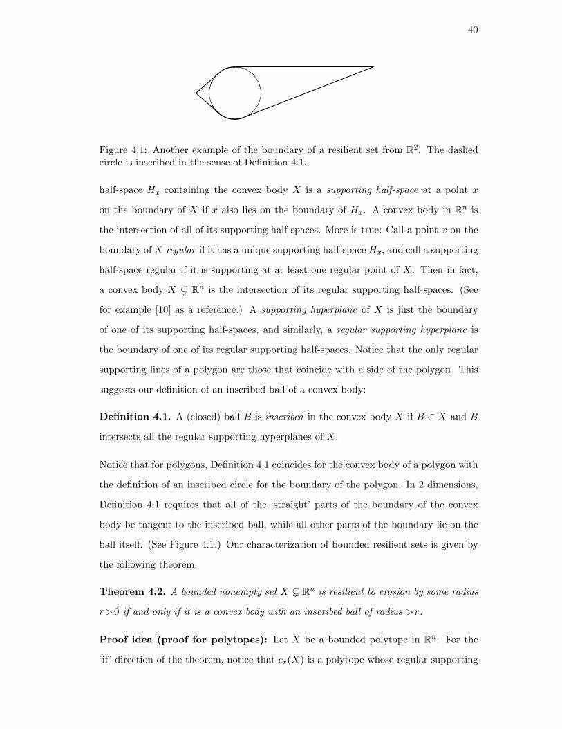
40
Figure 4.1: Another example of the boundary of a resilient set from R2. The dashedcircle is inscribed in the sense of Definition 4.1.
half-space Hx containing the convex body X is a supporting half-space at a point x
on the boundary of X if x also lies on the boundary of Hx. A convex body in Rn is
the intersection of all of its supporting half-spaces. More is true: Call a point x on the
boundary of X regular if it has a unique supporting half-space Hx, and call a supporting
half-space regular if it is supporting at at least one regular point of X. Then in fact,
a convex body X ( Rn is the intersection of its regular supporting half-spaces. (See
for example [10] as a reference.) A supporting hyperplane of X is just the boundary
of one of its supporting half-spaces, and similarly, a regular supporting hyperplane is
the boundary of one of its regular supporting half-spaces. Notice that the only regular
supporting lines of a polygon are those that coincide with a side of the polygon. This
suggests our definition of an inscribed ball of a convex body:
Definition 4.1. A (closed) ball B is inscribed in the convex body X if B ⊂ X and B
intersects all the regular supporting hyperplanes of X.
Notice that for polygons, Definition 4.1 coincides for the convex body of a polygon with
the definition of an inscribed circle for the boundary of the polygon. In 2 dimensions,
Definition 4.1 requires that all of the ‘straight’ parts of the boundary of the convex
body be tangent to the inscribed ball, while all other parts of the boundary lie on the
ball itself. (See Figure 4.1.) Our characterization of bounded resilient sets is given by
the following theorem.
Theorem 4.2. A bounded nonempty set X ( Rn is resilient to erosion by some radius
r>0 if and only if it is a convex body with an inscribed ball of radius >r.
Proof idea (proof for polytopes): Let X be a bounded polytope in Rn. For the
‘if’ direction of the theorem, notice that er(X) is a polytope whose regular supporting

41
hyperplanes are parallel to to the regular supporting hyperplanes of X and, like regular
supporting hyperplanes of X, are at constant distance from the center of the inscribed
ball of X. This implies that er(X) is similar to X.
For the other direction, we have that er(X) = σ(X) for a similarity transformation
σ. First note that X must be convex; otherwise, er(X) is not even a polytope. So long
as X is convex, er(X) is another polytope, and each regular supporting hyperplane H
of er(X) is parallel to, and at distance r from, a regular supporting hyperplane H of
X. Since X and er(X) are similar, they have the same finite number of sides, and so
every regular supporting hyperplane of X is such a H. Letting p denote the fixed point
of σ, we have d(H, p) = d(H, p)− r for all regular supporting hyperplanes H of er(X).
Therefore, for the lists of distances {d(H, p)} and {d(H, p)} to be the same up to a
scaling factor, we must have that they are both lists of constant distances; i.e., that the
regular supporting hyperplanes of each lie at constant distances from p.
The proof of Theorem 4.2 is the subject of Section 4.1, and, in light of the simplic-
ity of the characterization, is suprisingly technical. The first hole in the above ‘proof
idea’ when applied to general bounded sets is showing that they must be convex; this
is easy to accomplish, however. The second (more annoying) snag is that when the
number of regular supporting hyperplanes is not finite, it does not seem straightfor-
ward to argue that all regular supporting hyperplanes of X must be parallel to regular
supporting hyperplanes of er(X) (in fact, we carry out the complete proof of Theorem
4.2 without showing this to be the case, though it is an immediate consequence of the
Theorem). This difficulty arises because of the prospect of similarity under nonhomo-
thetic transformations (i.e., transformations that include nontrivial rotations). Though
it may seem intuitively natural that sets which are resilient must be so under homo-
thetic transformations, we will see in Section 4.3 that, without some assumptions like
boundedness or convexity, there are in fact sets X ⊂ Rn where er(X) = σ(X), but only
for transformations σ which include an irrational rotation.
As we will discuss in Section 4.3, unbounded resilient sets may be nonconvex and

42
quite complicated geometrically, and unlikely to satisfy any simple geometric character-
ization like that given in Theorem 4.2. Nevertheless, we can prove a simple geometric
characterization of (possibly unbounded) resilient sets which are convex; this is the
subject of Theorems 4.10, 4.11, and 4.12.
Resilient sets which are nonconvex behave in a counterintuitive way: eroding them
makes them ‘bigger’, in that the corresponding similarity transformation is distance-
increasing. To complete our characterization, we will see in Section 4.3.1 that a set
is resilient to erosion in this distance-increasing way if and only if it is the erosion of
a scale-invariant set (one which is self-similar under non-isometric transformations),
giving a surprising connection with ‘exact fractals’.
There is another operation closely related to the erosion operation, which we call
the expansion by a radius r, defined as
Er(X) =x∈X
B(r, x). (4.2)
Again B(r, x) denotes an open ball, thus Er(X) is always an open set. Notice that
we have er(X) = Er(XC)C , thus, in general, the erosion operation is equivalent to
the expansion operation by taking complements. Nevertheless, the family of convex
expansion-resilient sets is much less rich than that of convex erosion-resilient sets. For
example, it is not too hard to see that the only bounded expansion-resilient sets are
open balls. We give the characterization of all convex expansion-resilient sets in Section
4.2.3.
4.1 The bounded case
We first show the ‘if’ direction of Theorem 4.2: as noted above, a convex body X
containing a ball B of radius R intersecting its regular supporting hyperplanes is deter-
mined up to similarity by the selection of the positions of the points on the ball where
these intersections occur. The important point is that, up to the scaling of the ball,
these positions are unchanged by the erosion operation.
To make this precise, observe that the erosion er(X) of X by a radius r < R contains

43
the ball B′ = er(B) of radius R′ = R − r. Also, note that er(X) is the intersection of
the erosions er(H) of the regular supporting half-spaces H of X. The erosion er(H)
by r of any supporting half-space H of X tangent to B will be tangent to B′, and the
position of the point where the boundary of (er(H)) intersects B′ is the same as the
point where the boundary of H intersects B, apart from the scaling of the ball, since
the point where a half-space is tangent to a ball is determined by the orientation of
the half-space. Thus er(X) is the intersection of some half-spaces which are the images
of the regular supporting half-spaces of X under some fixed dilation, and so er(X) is
similar to X under that same dilation.
For the other direction, we will first work to show that if X is resilient and bounded,
then it must be convex. (This is not the case if we drop the unbounded requirement.)
To do this, it suffices to show that if a nonconvex set undergoes erosion, some distance
associated with it increases (making it impossible that it is similar to the original set
under a distance-decreasing similarity transformation). We call the associated ‘distance’
we use the ball-convexity :
Definition 4.3. The ball-convexity bc(X) of a closed set X ( Rn is the supremum of
radii R for which the complement of X is a union of open balls of radius R.
The ball-convexity of a set provides a kind of measure of its convexity: note that any
convex body X satisfies bc(X) =∞, since the complement of any convex body can be
written as the union of open half-spaces, which can be in turn written as the unions of
balls of arbitrarily large radii.
What about the converse? It is not true in general that a set with infinite ball-
convexity is convex: for example, any closed set X ⊂ R2 lying entirely on some line has
infinite ball convexity, even though many such sets are not convex. This the only kind
of counterexample, however:
Observation 4.4. A closed set X ( Rn which does not lie in any (n− 1)-dimensional
subspace is convex if and only if bc(X) =∞.
Proof. As already pointed out, the ‘only if’ direction is clear. For the other direction,
assume X is not convex. So there are points x1, x2 ∈ X such that the line segment

44
b
b
bX
x1
x3
x2
b q B(ε, q)
b p
b
R
Figure 4.2: Proving the ‘if’ direction of Observation 4.4 for the dimension n = 2; thedistance R is a upper bound on the ball-convexity of X; balls of any larger radiuscannot include the point p without also including points of X.
(x1, x2) includes a point q not in X. Since X is closed, in fact there is a ball B(ε, q)
about the point q which contains no points of X.
Since X doesn’t lie entirely in some (n−1)-dimensional subspace, we can choose ad-
ditional points x3, x4, . . . xn+1 ∈ X so that the convex hull of all the points x1, . . . , xn+1
is an (n + 1)-simplex. Now choose a point p from B(ε, q) which lies inside the (n + 1)-
simplex (but not in X).
Let R the maximum of the radii of the n+ 1 (n− 1)-spheres determined by (n+ 1)-
tuples from the set {p, x1, x2, . . . , xn+1}. Then we have that bc(X) ≤ R, since a ball
of radius > R cannot include the point p without including one of the points xi ∈ X.
(This situation for n = 2 dimensions is shown in Figure 4.2.) In particular, bc(X) <∞,
as desired.
Armed with the concept of ball convexity, it easy to show:
Lemma 4.5. Let er(X) = σ(X) for some r > 0 and some similarity transformation σ.
Then X must be convex, unless the transformation σ is distance-increasing.
Proof. Since X is resilient, it is closed and does not lie in any (n − 1)-dimensional
subspace (unless it is empty). Also, if bc(X) is finite, then we have that bc(er(X)) ≥

45
bc(X) + r. Thus we are done by Observation 4.4, since for bc(X) to be finite, σ would
have to be distance-increasing.
The similarity transformation corresponding to the erosion of a bounded resilient set
is always distance-decreasing since, for example, the diameter decreases upon erosion.
Thus Lemma 4.5 implies that bounded resilient sets must be convex. Since a convex
body is the intersection of its supporting half-spaces (and even of just its regular ones),
we can therefore study the erosion operation by examining its effect supporting half-
spaces/hyperplanes.
First note that the erosion of an intersection equals the intersection of the erosions:
er(Aα) =
er(Aα) for any family of subsets Aα ⊂ Rn (this is easily deduced from
line (4.1)). Since a convex body X is the intersection of its supporting half-spaces, we
have for any regular supporting half-space H of X that er(X) ⊂ er(H). Thus, if some
point on the boundary of er(X) is at distance r from the boundary of H, we have that
er(H) is in fact a supporting half-space to er(X) at the point x. Of course, any point
x on the boundary of er(X) must lie at distance r from some point x on the boundary
of X; we see that if x has a unique supporting half-space, then so must x:
Observation 4.6. If X ( Rn is closed and convex, then any regular point x on the
boundary of er(X) is at distance r from a (unique) x on the boundary of X which is
regular. The unique supporting hyperplane at x of er(X) is a parallel to the unique
supporting hyperplane of X at x.
Theorem 4.2 will imply that any bounded resilient set X is in fact resilient to erosion
by all radii r for which er(X) has positive diameter. For the proof of the Theorem, we
want to at least know that a bounded resilient set can be eroded to an arbitrarily small
copy of itself. First observe the following:
Observation 4.7. For any similarity transformation σ with scaling factor α, we have
σ(er(X)) = eαr(σ(X)).
Observation 4.7 captures the way in which the erosion of a resilient set is again resilient
to erosion. If X is resilient to erosion by the radius r, then er(X) = σ(X), so that Ob-
servation 4.7 gives us that eαr(er(X)) = σ2(X). By the triangle inequality, eαr(er(X))

46
is just er+αr(X), so we get that in addition to being resilient to erosion by the radius
r, X is also resilient to erosion by the radius r + αr, with corresponding similarity
transformation σ2. Repeating this argument in the natural way gives us the following
observation:
Observation 4.8. If er(X) = σ(X) for some similarity transformation σ with scaling
factor α, then it is resilient to erosion by
ri =
0≤k<i
rαk (4.3)
for all i; the corresponding similarity transformation is σi.
Our final piece of preparation concerns spherical subsets which are isomorphic to
proper subsets of themselves:
Observation 4.9. Let A ⊂ B be subsets of the sphere Sn−1, such that φ(A) = B,
where φ is some isometry of the sphere. Then A is dense in B.
Proof. Otherwise, let some neighborhood U of a point b ∈ B contain no points of A.
Then φ−1(U) contains no points of B, and so again no points of A. But then φ−2(U)
contains no points of B and so no points of A, etc.: we have that φ−k(U) contains no
points of B (or A) for any k ∈ Z+.
On the other hand, for the contradiction, we claim that for any ε, we can always
find some k ∈ Z+ so that φ−k(b) is at distance < ε from b. Certainly, among all of
the images φ−1(b), φ−2(b), φ−3(b) . . . , there must be a pair φ−i(n), φ−j(n) (i < j) at
distance < ε (possibly, the distance is 0). Applying φi, we have that b is at distance
< ε from φ−j+i(b).
We are now ready to prove Theorem 4.2. In fact, we are ready to prove a more
general statement, which includes Theorem 4.2 as a special case, but also makes up an
important part of the characterization of (possibly unbounded) convex resilient sets:
Theorem 4.10. Let X be a (possibly unbounded) nonempty proper subset of Rn. Then

47
H = H
H ′ri
X
σi(X)
(a) The situation in the case where σis just a homothety (i.e., it does notinclude a rotational component). HereH is parallel to H ′, so H = H.
H ′
ri
H
HX
σi(X)
(b) The situation where σ may includea rotation. Notice that, as drawn, H isnot parallel to any regular supportinghyperplane of eri(X).
Figure 4.3: Proving Theorem 4.10. In both cases, H ′ is the image of H under σi.
we have σ(X) = er(X) for some r and some distance-decreasing similarity transforma-
tion σ if and only if X is a convex body with an inscribed ball of radius > r.
Proof. Given that er(X) = σ(X), Observation 4.8 gives us that X is resilient to erosion
by the radii r1, r2, r3, . . . defined by the partial sums in line (4.3), with corresponding
similarity transformations σ, σ2, σ3, . . . , respectively. Let R = sup(ri) =∞
k=0 rαk, and
let p be the fixed point of the similarity transformation σ. X is convex by Lemma
4.5. We will prove Theorem 4.2 by demonstrating that the boundaries of all regular
supporting half-spaces H of X lie at distance R from the point p. Note that any
supporting hyperplane of X must lie at distance ≥ R from p, since eri(X) must contain
the point p for every ri (since p is fixed by σ); we need to show that all of the regular
supporting hyperplanes of X lie at distance ≤ R from p.
Since we are not assuming that X is bounded, we do not assume even that the
regular supporting hyperplanes of X are at bounded distance from p. To keep this
from causing problems, we fix some number D > R + 1, and focus on the set HD of
regular supporting hyperplanes of X lying within distance D of X. We will show that
for any H in HD, we actually have that H lies at distance ≤ R from p. Since D > R+1
can be chosen arbitrarily, this implies the Theorem.

48
Because hyperplanes in HD lie at bounded distance from p, we can choose i suffi-
ciently large so that all the images σi(H), (H ∈ HD) lie within any positive distance ε
from the point p. Note that each such hyperplane H ′ = σi(H) (H ∈ HD) is a regular
supporting hyperplane of eri(X). Thus, by Observation 4.6, there is a regular support-
ing hyperplane H of X lying parallel to and at distance ri from H ′. Since H ′ is at
distance < ε from p, H is at distance < ri + ε from p, and thus at distance < R + ε.
Let HiD = {H H ∈ HD}. Note that by choosing ε < 1, we have R + ε < D, thus, in
particular, HiD ⊂ HD.
Since HiD consists of hyperplanes within distance R + ε of p, we would be done (by
letting ε go to 0) if we could assert that HD = HiD for all i. This is certainly the case
if σ doesn’t include a rotation and consists just of the homothety x →→ α(x− p) + p. In
this case, given any regular supporting hyperplane H of X, its image H ′ = σ(H) is a
regular supporting hyperplane of eri(X) which is parallel to H, and therefore we have
that H = H (this situation is shown in Figure 4.3(a).
Since we do not assume that σ is homothetic, we allow that HiD ( HD; i.e., that
there are regular supporting hyperplanes of X not parallel to any regular supporting
hyperplane of eri(X). Figure 4.3(b) shows this hypothetical situation. Let ν(H) denote
the unit normal vector of any supporting hyperplane H of X, (oriented towards X,
say). Since σ is distance-decreasing, it has a fixed point p, and can be written as the
product of a homothety and an isometry, which both fix p. The isometry induces an
isometry φ of the unit sphere Sn−1, and we have that ν(H) = φ(ν(H)). Thus, the
set of the orientations of regular supporting hyperplanes of X which are parallel to
regular supporting hyperplanes of eri(X) is the image under the rotation φ of the set
of the orientations of all regular supporting hyperplanes of X. Thus by Observation
4.9, the set of orientations of regular supporting hyperplanes H which are parallel to
regular supporting hyperplanes of eri(X) is dense in the set of orientations of all regular
supporting hyperplanes of X. In other words, for any regular supporting hyperplane H
of X and for any ε′ > 0, we can find another regular supporting hyperplane H0 of X
at dihedral angle θ < ε′ to H, which is parallel to some regular supporting hyperplane
H0 of eri(X), and thus lies at distance < R + ε from p.

49
θ
d
bc
H
H◦
B(R, p)< ε
Figure 4.4: Finishing the proof of Theorem 4.10. The shaded regions are the half-spacescorresponding to H and H0. X lies somewhere in their intersection.
To finish the proof, assume that some hyperplane H ∈ HD of X is at distance > ε
from the ball B(R, p) of radius R centered at p. We have that there is a hyperplane
H◦ ∈ HiD of X at an arbitrarily small dihedral angle θ to H. Since H◦ ∈ Hi
D, we have
that H◦ is within distance R + ε of p. Referring to Figure 4.4, we let c be the point on
the boundary of H which is closest to the point p, and let d be the distance between
c and the intersection H ∩ H◦. Any points on H at distance < D from c lie outside
of supporting half-space of X whose boundary is H◦, and so outside of X as well. By
choosing H◦ so that the angle θ is arbitrarily small, we can make d arbitrarily large;
thus no points on the boundary of H lie on X, and H cannot be a supporting half-space
to X after all. We conclude that all regular supporting half-spaces of X lie at distance
R from p.
4.2 The general convex case
In this section we consider the case of general (i.e., possibly unbounded) convex resilient
sets; our aim is to characterize these sets in simple geometric terms. Theorem 4.10
already provides a characterization for the case where er(X) = σ(X) and σ is distance-
decreasing. Two cases remain for our geometric characterization of convex resilient
sets: the case where σ is an isometry, and the case where σ is distance-increasing.
These cases are covered in Section 4.2.2. First, we consider some examples from R3
which demonstrate that Theorem 4.10 isn’t the complete story, and that all of these
possibilities really can occur. (It is not too hard to check that at least 3 dimensions are
required to have examples of convex resilient sets not covered by Theorem 4.10.)

50
(a) X1 (b) X2 = er(X) (c) X3 = er(X2)
Figure 4.5: X1 is resilient under distance-decreasing transformations. X2 is not resilientto erosion. X3 is resilient under distance-increasing transformations.
4.2.1 Unbounded convex examples in R3
In this section we give an example of a convex set X1 such that X1 is resilient under
a distance-decreasing similarity transformation and so has an inscribed ball, er(X1) is
not resilient, and such that e2r(X1) is resilient under a distance-increasing similarity
transformation (and has no inscribed ball).
Let X1 be the ‘bottomless tent’ depicted in Figure 4.5(a). X1 is the unbounded
intersection of four half-spaces Hi, chosen so that ∂H1 ∩ ∂H3 ∩ X1 is a line segment
(here ∂Hi denotes the boundary), while Hi ∩ Hj ∩ X1 is a ray whenever j ≡ i + 1
(mod 4). The half-spaces are chosen so that the dihedral angle between H2 and H4 is
greater than that between H1 and H3, and such that any horizontal cross section is
rectangular.
X1 has an inscribed ball, as depicted in Figure 4.5(a). Thus X1 is resilient to erosion
by radii less than the radius r of the ball; X2 = er(X1) is depicted in Figure 4.5(b). It
is not resilient and so has no inscribed ball.
If we erode X2 by the radius r, we get the convex body X3 depicted in Figure 4.5(c).
It has no inscribed ball, but is nevertheless resilient: the erosion of X3 by any positive
radius r satisfies er(X3) = σ(X3) for some similarity transformation σ which increases
distances.
Finally: what if in Figures 4.5(a) or 4.5(c) the dihedral angles between the two
pairs of opposite half-spaces had been equal? Like X3, the result X4 would not have

51
an inscribed ball, but would still be resilient. In fact, for all r > 0, we would have
σ(X4) = er(X4) where σ is now a translation.
4.2.2 Characterizing all resilient convex bodies in Rn
We say that a convex body X has an exscribed ball of radius r > 0 centered at a point
p if all of its regular supporting half-spaces are at distance r from p (in particular, p
lies outside of all of them). Note that, in general, the distance between X and p may
be greater than r.
This concept allows us to extend the characterization in Theorem 4.10 to convex
sets for which er(X) = σ(X), where r > 0 and σ is a distance-increasing similarity
transformation.
Theorem 4.11. An (unbounded) convex body X ( Rn satisfies er(X) = σ(X) for some
r > 0 and a distance-increasing similarity transformation σ if and only if X has an
exscribed ball.
Thus, in particular, the example X3 from Section 4.2.1 has an exscribed ball.
The final piece of our characterization of convex resilient sets (covering for example
the set X4 from Section 4.2.1) is the following theorem.
Theorem 4.12. An (unbounded) convex body X ( Rn satisfies er(X) = σ(X) for some
r > 0 and an isometry σ if and only if all regular supporting hyperplanes of X lie at
some common dihedral angle = π2 to some fixed hyperplane.
(By Lemma 4.5, the convexity assumption is superfluous in Theorem 4.12.)
For Theorems 4.11 and 4.12, the ‘if’ directions are straightforward. Below we prove
the ‘only if’ directions for each.
Proof of Theorem 4.11
We are striving to show that all of the regular supporting half-spaces of X are at a
common distance from some point external to all of them. We first have to show that
there is such an external point. The following lemma shows that the fixed point of σ
must be external to every half-space.

52
cb
pb
D
θH
H◦i
Figure 4.6: (Proving Lemma 4.13.)
Lemma 4.13. If a convex body X ( Rn satisfies er(X) = σ(X) for some r > 0 and a
distance-increasing similarity transformation σ, then the fixed point p of σ lies outside
of every supporting half-space of X.
Proof. Write σ = γ ◦ φ, where γ is a homothety, φ is rotation (an isometry of Sn−1),
and σ, γ, and φ all have the same fixed point. Let H be a supporting half-space of X
which contains the fixed point p of σ. Similar to the end of the proof of Theorem 4.10,
our aim is to ‘separate’ H from X by nearly parallel half-spaces which are also regular
supporting half-spaces to X.
As before, let ri =i−1
k=0 αkr. Since eri(X) ⊂ H for all i, eri(X) has a (not
necessarily regular) supporting half-space H∗i which is parallel to H. Since α > 1,
the ri’s get arbitrarily large as i increases, so we have for sufficiently large i—say,
i > K for some K > 0—that p lies outside of H∗i . Now, since H∗i is a supporting
half-space of eri(X), H◦i = σ−i(H∗i ) is a supporting half-space to X. The important
point is that p must also lie outside of H◦i , since it lies outside of H⋆i , and σ fixes p.
Thus, letting c denote the point on the boundary of H which is closest to p, we have
that points on the boundary of H within the distance D between p and the intersections
of the boundaries of H and H◦i lie outside of H◦i , and so outside X (see Figure 4.6).
This distance can be made arbitrarily large by choosing i so that θ is arbitrarily small,
thus we get that there are no points on the boundary of H from X, thus H is not
supporting to X, a contradiction.
We can now prove Theorem 4.11. Note that the distances between p and the regular
supporting half-spaces of X are bounded by the distance between p and X. Thus, by
choosing i sufficiently large, Lemma 4.11 implies that we can ensure that all of the

53
images σ−i(H) of regular supporting half-spaces H of X lie within distance ε of p
for any positive ε. By Observation 4.7 we have that X = eri/αi(σ−i(X)). Thus by
Observation 4.6, every regular supporting half-space of X is at distance riαi from a
regular supporting half-space of σ−i(X); thus, all regular supporting half-spaces of X
are at distance < riαi
+ ε from p. Taking the limit as i goes to infinity, we get that any
regular supporting half-space of X is at distance rα−1 from the point p.
Proof of Theorem 4.12
Any isometry can be written as the commutative product τ · φ of a translation and
rotation (by rotation we mean any isometry with a fixed point). (A proof of this fact
can be found in [15], p. 217.) Under the conditions of Theorem 4.12, we have that X is
collapsible by arbitrarily large radii, so it is easy to see that σ can have no fixed point:
such a point cannot lie inside X, since then sufficiently large radii would erode X to
the point where it does not contain it; if it lies outside on the other hand, the distance
between it and X increases with erosion.
Thus τ is nontrivial. Since the product τ ·φ commutes, we have that the rotation φ
must fix the direction ντ of the translation τ , thus all of the points on a line L = p+ντx,
x ∈ R, where p is a fixed point of φ.
Eroding a half-space by any radius gives a half-space similar to the first under
a translation. In fact, similarity can be under a translation in any direction of our
choice (except along a vector lying inside any hyperplane parallel to the boundary); the
magnitude of the translation then depends just on the radius of collapse and the angle
between the direction of the translation and the half-space in question. (We take as
the angle between a half-space and a vector the angle between the normal vector of the
half-space and the vector). Thus the pair r and the magnitude |τ(0)| of the translation
τ together determine a unique angle θτ,r, which is the angle a half-space H must lie at
relative to the vector ντ for us to have that er(H) = τ(H). If we have that φ is trivial,
so that σ = τ , then it follows easily (using Observation 4.6) that all regular supporting
half-spaces of the set X must lie at the angle θτ,r to ντ , as desired: basically, they
must all get ‘pushed’ by the erosion in the direction ντ at the same rate. We will now

54
Lb
q
bτkH(q)
kr
D
θ
H
H
σk(H)
Figure 4.7: (Finishing the proof of Theorem 4.12.)
show this is true even if φ is nontrivial. First we point out that X must intersect L:
otherwise, the distance between L and X increases with erosion, contradicting that σ is
an isometry fixing L. This implies that no supporting half-space of H can be at angle
π2 to ντ , since then, for a sufficiently large k, ekr(H) would not intersect the line L, and
so neither would ekr(X).
If H is a regular supporting half-space to X, let θH denote its angle to the vector ντ .
We first claim that we must have that θH ≤ θτ,r. Otherwise, if θH > θτ,r, we have that
er(H) = τH(H) where τH is a translation in the direction ντ but with strictly greater
magnitude: |τH(0)| > |τ(0)|. Let q be the point where L intersects δH (we cannot have
L ⊂ δH since, as noted above, their angle cannot be π2 ).
Observe that the distance between q and ekr(X) ∩ L is just the original distance
between q and X ∩ L, plus the magnitude of the translation τk:
d(q, ekr(X) ∩ L) = k|τ(0)|+ d(q,X ∩ L). (4.4)
On the other hand, we have that ekr(X) ⊂ ekr(H) = τkH(H), and for suitably large
k we have that d(q, τkH(H)) > k|τ(0)| + d(q,X ∩ L), contradicting line (4.4). (Notice
that this part of the argument has not used the regularity of H; X cannot have any
supporting half-spaces at angles > θτ,r from ντ .)
Now we wish to show that θH ≥ θτ,r. Assume the contrary. Let again q be the
intersection point of L with the boundary of H, and again let τH be the translation in
the direction ντ satisfying er(H) = τH(H).
Let H ′ = σk(H) for some k. We have that H ′ passes through τkH(q), which lies at

55
distance k|τH(0)| from q. Observation 4.6 implies that X has a regular supporting half-
space H parallel to H ′, with d(H,H ′) = kr. The important point is that the distance
between q and τkH(q) is greater than kr, and ever more so as we increase k. Therefore,
referring to Figure 4.7, we can make the distance D between the boundary of H and
the intersection of the boundaries of H and H arbitrarily large by choosing k so that
the angle θ is small. We conclude that no points on the boundary of H can intersect
X, a contradiction.
4.2.3 Convex sets resilient to expansion
While, in general, asking about erosion and expansion are equivalent by taking com-
plements, it is natural to wonder about the family of convex sets resilient to expansion,
i.e., convex sets X for which Er(X) = σ(X) for some r > 0, and some similarity trans-
formation σ. It turns out that this family is not as rich as the corresponding family
for erosion. In particular, any convex expansion-resilient set is also erosion-resilient;
moreover, as is not hard to verify, the only bounded sets resilient to expansion are open
balls. The following gives the characterization of all convex sets resilient to expansion:
Theorem 4.14. A (possibly unbounded) convex nonempty proper subset of Rn is re-
silient to expansion by some radius r if and only if it is open and all of its supporting
half-spaces are at a common distance R > r from some point.
For the purposes of Theorem 4.14, we say that the supporting half-spaces of an open
convex set are the interiors of the supporting half-spaces of its closure.
Proof of Theorem 4.14: (Sketch) Check that the closure of a convex expansion-
resilient set is also erosion-resilient (since if X is convex and closed, then we have
er(Er(X)) = X). Additionally, all of its supporting half-spaces must be regular (since
this is true after an expansion). By examining the characterizations given in Theorems
4.11 and 4.12, this rules out that a similarity transformation corresponding to the
erosion of X is either distance increasing or distance-preserving (unless X is just a
half-space, in which we are done); therefore, the characterization of Theorem 4.10
applies. Since all of the supporting half-spaces to X must be regular, this completes

56
the proof.
4.3 The nonconvex case
We begin this section by giving examples of the ‘strange behaviors’ nonconvex (and so
unbounded) resilient sets can exhibit; in Section 4.3.1, we show how these sets can be
characterized.
Example 4.15
Our first example lies in R1. It seems ‘fractal-like’, and is resilient to erosion by arbitrar-
ily large radii, even though every component of the set has finite diameter. Moreover,
the set {ri} of radii by which it is resilient to erosion is discrete. As we will see in the
next example, this kind of 1-dimensional resilient set can be used to create sets with
similar properties in higher dimensions.
We find it easiest to describe the complement of the set. To this end, let T =
{4,−4, 28,−28, 196,−196, . . . } be the set of integers of the form ±4 · 7k, k ≥ 0, and let
A be the set of of all numbers A for which
n =t∈Ta
x
for some subset Ta ⊂ T . So, for example, A includes the points
0,±4,±24,±28,±32,±164,±168,±172,±192,±196,±200,±220,±224,±228,
etc. Let now Y = E1(A) be the expansion of A by radius 1, and let X = Y C be the
complement of Y . Then X is resilient to erosion by a radius 2 · 7k for every k ≥ 0. The
erosion by radius 2 is shown in Figure 4.8.
We will sketch the proof of this fact in terms of the expansion of Y , rather than
the erosion of X, so we will prove that E2(Y ) ∼ Y ; in fact, that E2(Y ) = 7 · Y ,
where [·] here indicates pointwise multiplication. This is equivalent to showing that
E3(A) = 7 · E1(A).

57
50 100 150 200−50−100−150−200 0
X
Z
Figure 4.8: Shown are portions of X and its erosion Z = e2(X) by the radius 2.
Let p ∈ E1(A). Then d(p, a) < 1 for some
a =t∈Ta
t, (4.5)
where Ta ⊂ T . Multiplying by 7, we get that all points p′ of 7 · E1(A) are within < 7
units of a point a′ of the form
a′ =t∈T ′
t (4.6)
for some T ′ ⊂ 7 · T . But T = (7 · T )∪{4,−4}. Thus we have that p′ must be within
distance < 7− 4 = 3 of a point of A; thus we have that 7 · E1(A) ⊆ E3(A).
For the other direction, let now p ∈ E3(A). So d(p, a) < 3 for some a satisfying
line (4.5) for some Ta ⊂ T . Thus d(p, a′) < 7 for some a′ satisfying line (4.6) for
T ′ ⊂ T \ {4,−4} = 7 · T . Thus 17p is at distance < 1 from a point of T , and so we have
shown that E3(A) ⊆ 7·E1(A). Combining the two directions, we have E3(A) = 7·E1(A),
as desired.
Example 4.16
Recall that the erosion of an intersection is the intersection of the erosions. Thus,
taking the intersection of sets Xi all satisfying σ(Xi) = er(Xi) for fixed r, σ, gives
another resilient set. (Equivalently, we can make examples of expandable sets from other
suitable expandable sets by taking unions instead of intersections.) Using this basic
method, we can create in Rn diverse classes of examples of unbounded sets displaying the
same properties as the example we have given in R1. Figure 1.3 from the Introduction
(page 8) illustrates an unbounded resilient set in R2 constructed from four rotated
copies of the product X × R, together with the set {z ∈ R2 s.t. ∥z∥ ∈ X}, a circular
variant of X.

58
Example 4.17
This example is based on the classical logarithmic spiral, given in polar coordinates
by R(θ) = aebθ. The logarithmic spiral has the remarkable property that it is self-
similar under similarity transformations (centered at the origin) which take on all scaling
factors α > 0, while the rotational component of the similarity transformation varies
continuously with the choice of α.
To get our example, we modify this spiral by giving it a ‘truncated’ logarithmic
thickness: more precisely, let R0(θ) = aebθ and T0(θ) = ebθ − 1, and let
S1 =θ
B(T0(θ), (R0(θ); θ)), (4.7)
where B(T0(θ), (R0(θ); θ)) is the closed ball of radius T0(θ) about the point (R0(θ); θ),
given in polar coordinates. Then S1 is resilient to erosion by any radius. In general, the
similarity transformation includes a rotation which varies continuously with the choice
of the radius of erosion. (S1 is shown in Figure 4.9, with two of its erosions). The
resiliency of S1 will follow from our characterization of resilient sets in the next section.
Example 4.18
Fix some similarity transformation σ centered at the origin which increases distances
and includes an irrational rotation. Fix the body T of some rectangle, and let Q0 be the
union of all the images σi(T ), over all integers i. Then the erosion Qr = er(Q0), shown
in Figure 4.10, is resilient to erosion by a discrete set of radii, starting with the radius
r(α− 1); each erosion induces a similarity transformation which includes an irrational
rotation. Again, similarity will follow from Theorem 1.5.
4.3.1 Characterizing nonconvex resilient sets
To finish our characterization of resilient sets, we need to cover nonconvex sets; by
Lemma 4.5, it is enough to cover the case where the similarity transformation corre-
sponding to erosion is distance-increasing. In light of the examples in the previous sec-
tion, it is clear that the characterization for this case will not be of the simple geometric

59
Figure 4.9: Sr is a logarithmic spiral with ‘truncated’ logarithmic thickness, and isresilient to erosion by any radius; the corresponding similarity transformation includesa rotation by an angle determined by the radius of erosion. (Two arbitrary erosions areshown.)
Figure 4.10: Qr is a discrete ‘spiraling’ resilient set. It is shown with its second erosionin black.

60
type given for the distance decreasing and isometric cases. Instead, the characteriza-
tion will show that any resilient set whose corresponding similarity transformation is
distance increasing can be constructed essentially in the same way as we constructed
Example 4.18, and moreover, all such constructions lead to resilient sets. Let’s make
this more precise:
Definition 4.19. A set W ⊂ Rn is scale-invariant if we have W = σ(W ) for a similarity
transformation σ with scaling factor α > 1.
Notice now that Q0 from Example 4.18 is a scale-invariant set, thus Qr was con-
structed as the erosion of a scale-invariant set. Theorem 1.5, restated below, tells
us that this feature characterizes all sets which are resilient under distance-increasing
similarity transformations:
Theorem 1.5 (restated). A set X ⊂ Rn satisfies er(X) = σ(X) for some distance-
increasing similarity transformation σ if and only if we have X = er/(α−1)(W ) for some
set W which is scale-invariant under σ.
In particular, note that the spiral from Figure 4.9 is the erosion of a scale-invariant
logarithmic spiral S0 with thickness T0(θ) = ebθ. Theorem 1.5 also implies that Exam-
ples 4.15 and 4.16 are the erosions of scale-invariant sets. In these cases, the original
self-similar sets are dense in R1 and R2, respectively. Notice that Theorem 1.5 overlaps
with Theorem 4.11 in its coverage of convex sets resilient to erosion with corresponding
distance-increasing similarity transformations. For example, in the case of the resilient
set X3 (Figure 4.5(c)) discussed in Section 4.2.1, the corresponding scale-invariant set
is the set X2 (Figure 4.5(b)).
For the proof of Theorem 1.5, let’s first see why the ‘if’ direction is true. We have
that W = σ(W ), where σ has scaling factor α > 1. Applying Observation 4.7 with
some radius r′ to the set W gives us that σ(er′(W )) = eαr′(σ(W )). Thus eαr′(W ) =
σ(er′(W )). But we have (by the triangle inequality) that eαr′(W ) = er′(α−1)(er′(W ));
thus we have that er′(α−1)(er′(W )) = σ(er′(W )). Thus, letting r = r′(α − 1), we have
that the set X = er′(W ) is resilient to erosion by the radius r.

61
For the other direction, we need to first construct the set W which should be scale
invariant and give rise to X under erosion. Observe that since X is similar to er(X),
Observation 4.7 gives us that X = er/α(σ−1(X)). In fact, we have the following obser-
vation, similar to Observation 4.8:
Observation 4.20. If er(X) = σ(X) for some similarity transformation σ with scaling
factor α, then for all i ≥ 1 and
r−i =
1≤k≤i
r
αk, (4.8)
we have X = er−i(σ−i(X)).
Motivated by this observation, we set W as
W =k≥1
σ−k(X); (4.9)
note that W is thus a scale-invariant set: we have σ(W ) = W .
To complete the proof, it just remains to check that er/(α−1)(W ) = X. Note that
rα−1 = sup(i≥1) r−i, thus we certainly have that er/(α−1)(W ) ⊃ X; otherwise, some
point of X must be at distance r0 < rα−1 from the complement of W . We would then
have for some sufficiently large i that r0 < r−i, a contradiction since er−i(σ−i(X)) = X,
yet σ−i(X) ⊂W .
So far, we have still not used that α > 1 (i.e., that σ is distance-increasing). Note
that without this assumption, the W he have constructed may well be all of Rn.
Thus it remains to show that er/(α−1)(W ) ⊂ X. It suffices to show that any point
in the complement XC is at distance < rα−1 from the complement WC .
Since X = er−1(σ−1(X)), we have by the definition of the erosion operation that
any point y0 ∈ XC must lie at distance < rα from some point y1 in the complement of
σ−1(X). Similarly, y1 must lie at distance < rα2 from a point y2 in the complement of
σ−2(X). Continuing in this manner, we get a sequence {yi}i≥0 where, for each i, yi lies
outside of σ−i(X), and the distance d(yi−1, yi) is less than rαi . Since α > 1, this is a

62
Cauchy sequence, and there is some limit point y∞. We have that
d(y0, y∞) <k≥1
r
αk=
r
α− 1,
thus it just remains to check that y∞ does not lie in W . If it does, then by line (4.9)
we have that y∞ ∈ σ−i(X) for some i. But then, for some sufficiently large j, we
have that r−j− r−i > d(yj , y∞), a contradiction since er−j−r−i(σ−j(X)) = σ−i(X), and
yj /∈ σ−j(X).
4.3.2 Fractals and erosion
Theorem 1.5 shows a direct correspondence between scale-invariant sets and resilient
sets with corresponding distance-increasing similarity transformations. Although there
is a connection between fractals and scale-invariant sets, these concepts are certainly
not the same. The family of scale-invariant sets includes sets such as lines, half-spaces,
and the figure X2 from Figure 4.5(b) which are certainly not ‘fractals’. Moreover, the
definition of a fractal given in [37] by Mandelbrot—a set whose Hausdorff dimension
is strictly less than than its covering dimension—includes many sets which are not
actually ‘self-similar’ in any exact sense.
Nevertheless, an important class of fractals (including well-known examples such
as Koch’s snowflake and Sierpinski’s triangle) is that of fractals generated by ‘Iterated
Function Systems’. Our goal in this section is to briefly point out how members of this
class can give rise to scale-invariant sets. For more background on Iterated Function
Systems, see, for example, [26].
An Iterated Function System is a list f1, f2, . . . ft of distance-decreasing similarity
transformations of Rn. Its ratio list is the list α1, α2, . . . , αt of scaling factors of the sim-
ilarity transformations. Any iterated function system has a unique nonempty compact
invariant set K satisfying
K = f1(K) ∪ f2(K) ∪ · · · ∪ ft(K). (4.10)

63
The similarity dimension of the iterated function system is the solution s to the equation
ti=1
asi = 1. (4.11)
We will see shortly that under a certain condition, the similarity dimension is the same
as the Hausdorff dimension, so that K will be a fractal in the sense of Mandelbrot’s
definition so long as s is strictly less than the covering dimension (in particular, if it
is not an integer). Note that Sierpinski’s triangle is the invariant set of an iterated
function system with ratio list (12 ,12 ,
12) and so has similarity dimension log 3
log 2 . Koch’s
curve is the invariant set of an iterated function system with ratio list (13 ,13 ,
13 ,
13), thus
has similarity dimension log 4log 3 .
We are trying to show how to get scale-invariant sets from fractals generated by an
iterated function system. Of course, given any set X and a similarity transformation
σ, the set
SIσ(X) =k∈Z
σk(X)
is a scale-invariant set. In general, however, SIσ(X) may not seem very related to the
original set X; it may very well turn out to be the whole space, for example.
In the case of the invariant set of an iterated function system where we let σ = f1,
say, we have that
SIf1(K) =k∈Z
fk1 (K) =
k∈Z−
fk1 (K) = K ∪
k≥0
2≤i≤k
f−k1 ◦ fi(K), (4.12)
suggesting that SIf1(K) will retain some of the appearance of the set K. The problem
is that, in general, K and
N(K) =k≥0
2≤i≤k
f−k1 ◦ fi(K)
may overlap, thus we are not guaranteed that SIf1(K) shares the ‘structure’ of K. The
open set condition (OSC) on iterated function systems, introduced by Moran [39], is a

64
condition which controls the extent of this overlap: it requires that there is an open set
U with fi(U) ⊂ U for all 1 ≤ i ≤ k, and fi(U) ∩ fj(U) = ∅ for i = j. One important
consequence of the open set condition is that the similarity dimension of the iterated
function system must coincide with the Hausdorff dimension of the corresponding in-
variant set; in particular, this allows the dimension to be easily computed in many
cases (OSC is satisfied for the well-known examples of mathematical fractals, such as
Sierpinski’s Triangle and the Koch curve). A recent result of Bandt, et al. (Corollary
2 in [2]) implies that if an iterated function system satisfies the OSC, then there is an
open set V which intersects the invariant set K nontrivially and is disjoint from N(K);
thus the intersection V ∩K will be identical to the intersection V ∩SIf1(K). Thus OSC
ensures that K and SIf1(K) share the same small-scale structure, in a certain sense.
The preceding remarks imply that any fractal coming from an iterated function
system satisfying the open set condition gives rise to a scale-invariant set which retains
the small-scale structure of the original fractal. Figure 4.11(a) shows a portion of the
scale-invariant extension of Sierpinski’s Triangle, and Figure 1.2(a) shows a portion of
the scale-invariant extension of the Koch curve. Since as fractals these sets have empty
interior, it is necessary to take complements before taking the erosion to get a nonempty
resilient set. Figure 4.11(b) shows the resulting resilient set produced from Sierpinski’s
Triangle. In the case of the unbounded version of Koch’s curve, the complement consists
of two components, which are each scale-invariant and thus can separately give rise to
scale-invariant sets. Figure 1.2(b) shows the resilient set produced by taking the erosion
of one of these components.
4.4 Further Questions
Since the concepts of erosion, expansion, and similarity make sense in an arbitrary
metric space, the question of resiliency could be studied in a wide range of settings.
(Note that our proof of Theorem 1.5 is actually valid in any complete metric space.)
There is a natural line of inquiry in Euclidean space suggested by Theorem 1.5,
however. Since this theorem makes its characterization in terms of scale-invariant sets,

65
(a) Sierpinski’s Triangle can be extended ad-infinitum to create a scale-invariantset.
(b) Sr = er(S) is the erosion of the complement of the unbounded version ofSierpinski’s Triangle, and is resilient to erosion by the radius r. The area removedby its first erosion is shown in gray.
Figure 4.11: Getting a resilient set from a fractal.

66
it is natural to wonder about the ‘behavior’ of such sets. In this case, a natural line
of attack seems to be from the standpoint of their transformation groups. Define the
self-similarity group of a set X as the group of similarity transformations σ satisfying
X = σ(X). What can we say about which groups appear in this way?
The case of isometric transformation groups has received considerable attention
because of its applications in crystallography (see e.g., [14], [12]). Because of the ap-
plication, attention is restricted in that case to discrete groups. For our application to
resilient sets, there are relevant scale-invariant sets like the thickened logarithmic spi-
ral S0 whose self-similarity groups really are not discrete. Nevertheless, the following
question puts a reasonable restriction on the self-similarity groups, which is necessary
anyway for the set to give rise to nonempty resilient sets:
Question 4.21. Which groups of similarity transformations occur as the self-similarity
groups of subsets of Rn with nonempty interior?
It seems likely that Question 4.21 is interesting even for small values of n.

67
Chapter 5
Winning strategies for sequence games from a Lefthanded
Local Lemma
In the Introduction, we referenced the classical ternary sequence constructed by Thue
in 1906, containing no adjacent identical blocks [52, 53]. (It is easy to see that there
can be no binary sequence even just of length 4 with this property.) To obtain Thue’s
remarkable ternary sequence, recursively define binary sequences Ti where T0 = 0, and
Ti+1 is constructed by replacing each 0 in Ti with the string 01 and each 1 with the
string 10. Thus T1 = 01, T2 = 0110, etc. Each Ti is the initial segment of Ti+1, so the
limit T∞ = limi→∞ Ti is a well-defined binary sequence
0110100110010110100101100110100110010110011010010110100110010110 . . . .
Thue observed that T∞ is overlap-free—no two overlapping intervals are identical—
since this property is preserved under the replacement operation described above. In
particular, this implies that T∞ is cube-free: it contains no 3 consecutive identical
blocks. Construct the sequence
2102012101202102012021012102012 . . .
by counting the number of 1’s between each consecutive pair of 0’s in T∞. Since T∞ is
cube-free, this is a ternary sequence. The fact that T∞ is overlap-free implies that this
sequence is square-free.
This concept has many interesting generalizations and suggests several directions of
research (see [18] and [30] for overviews of the area and discussions of open problems).
One such direction concerns requiring that any identical blocks be far apart, rather

68
than simply nonadjacent. This is the subject of the following conjecture of Dejean [19]:
Conjecture 5.1 (Dejean (1972)). For every c ≥ 5, there is an infinite c-ary sequence
where (for all n) any two identical blocks of length n are separated by at least (c− 2)n
terms.
The conjecture is now proved. After being confirmed for c ≤ 14 [38, 42, 43] and c ≥ 30
[13, 16], proofs of the remaining cases were announced by both Currie and Rampersad
[17], and Rao [45]. If one is concerned only with large identical blocks, a much stronger
restriction can be placed on the distance between identical pairs, even in a binary
sequence:
Theorem 5.2 (J. Beck (1981) [4]). For any ε > 0, there is some Nε and an infinite
0-1 sequence such that any two identical blocks of length n > Nε are at distance >
(2− ε)n.
Theorem 5.2, which is essentially best possible ((2− ε)n cannot be replaced by 2n),
was an early application of the ‘General’ (or ‘Asymmetric’) Lovasz Local Lemma; the
existence of the relevant 0-1 sequence is proved by showing that the probability that
a random finite sequence has the properties in question is positive, and then using
compactness to show the existence of a suitable infinite sequence. Note that no explicit
construction of such a sequence is known.
While sequences that have nonrepetitive properties like those guaranteed by Beck’s
Theorem 5.2 may be very scarce, we will show in this paper that they are nevertheless
very ‘attainable’, in a certain sense (although we do not know how!). Consider a game
(the binary sequence game) in which two players take turns choosing from the digits
{0, 1} to form an unending binary sequence (the first digit is chosen by Player 1, the
second by Player 2, the third by Player 1, etc.). Our first result is an analog to Beck’s
theorem, showing that we can construct highly nonrepetitive sequences even when faced
with an adversary.
Theorem 5.3. For any ε > 0, there is an Nε for which Player 1 has a strategy in the
binary sequence game which ensures that any two identical blocks of length n > Nε in
the resulting sequence will lie at distance > (2− ε)n/2.

69
Roughly speaking, Beck’s Theorem 5.2 asserts that we can build a binary sequence
where any large blocks are separated by exponentially large distance. Theorem 5.3
asserts that we can build such a sequence even if an adversary gets to choose every
other digit. (Of course, as we have surrendered control over ‘half’ the sequence, it is
not surprising that the base of the exponent is lower. We will see shortly that (2− ε)n2
is best possible here.) Surprisingly, the proof of Theorem 5.3 is also probabilistic; it is
based on an extension of the Local Lemma (Theorem 5.10), and is many steps removed
from any constructive argument. We use our extension of the Local Lemma to show
(nonconstructively) that Player 2 cannot have a winning strategy in a finite version of
the game; this implies (nonconstructively) that Player 1 has a winning strategy for any
finite version of the game; this, finally, implies via compactness (nonconstructively) the
existence of a winning strategy for Player 1 in the infinite version of the game. Needless
to say, Player 1’s winning strategy may be impossible to determine explicitly (it seems
it may not even have a finite description).
Player 1 can ensure exponential distance between long identical blocks even if he
is an ‘underdog’, playing a (1 : t) biased game where the second player makes t moves
between each move of Player 1. In this case we have the following:
Theorem 5.4. For any ε > 0, there is an Nε for which Player 1 has a strategy in the
(1 : t) biased binary sequence game to ensure that any two identical blocks of length
n > Nε in the resulting sequence will lie at distance > (2− ε)n/(t+1).
Thus Player 1 can obtain a highly nonrepetitive sequence even in the face of a
powerful adversary. As remarked earlier, we know of no explicit sequence in which long
identical blocks are exponentially far apart. Nevertheless, Theorems 5.3 and 5.4 can be
interpreted as showing that very ‘robust’ construction strategies for such sequences do
exist.
We note that Theorems 5.3 and 5.4 are actually essentially best possible: assume
Player 1 has a strategy in the (1 : t) biased binary sequence game to force any long blocks
of length n > N to be at distance > (2 + ε)n/(t+1), and let Player 2 employ the simple
strategy of always choosing the digit 0. We let S denote the 0-1 sequence produced

70
by the game, and let S′ denote the sequence consisting of just Player 1’s moves (so, it
consists of every (t+1)st term from S). Since all of Player 2’s moves are 0, the fact that
S contains no identical blocks of length n > N at distance > (2 + ε)n/(t+1) implies that
S′ contains no identical blocks of length n′ = n/(t + 1) at distance > 1t+1(2 + ε)n/(t+1).
For sufficiently large n (depending on ε) this implies that S′ contains no identical
blocks of length n′ within distance 2n/t+1 = 2n′. Thus the contradiction follows from
the same argument which shows that Beck’s theorem is essentially best possible: by the
pigeonhole principle, there must be two identical blocks of length n′ whose first terms
both lie among the first 2n′
terms of S′. Note that the same kind of reduction shows
that that Theorems 5.3 and 5.4 are in fact generalizations of Beck’s Theorem 5.2 (even
for any fixed value of t, in the latter case).
Another result proved with the Local Lemma and related to Beck’s theorem is the
subject of Exercise 2 in Chapter 5 of the Alon-Spencer book [1], which asserts that for
any ε > 0 there is an Nε and a {0, 1} sequence α1, α2, α3, . . . in which any two adjacent
blocks αk+1, . . . , αk+n and αk+n+1, . . . , α2n, each of length n > Nε, differ in at least
(12 − ε)n places (so αk+j = αk+n+j for at least (12 − ε)n values of j between 1 and n).
(It is not hard to check that this is essentially best possible; begin with the observation
that any binary coloring of a complete graph is ‘bad’ on more than half the edges.)
Using the same extension of the Local Lemma used to prove Theorem 5.3, we prove the
following game-theoretic version of this result.
Theorem 5.5. For any ε > 0, there is an Nε such that Player 1 has a strategy in the
(1 : t) biased binary sequence game to ensure that any two adjacent blocks of length
n > Nε differ in at leastÄ
12t+2 − ε
än places.
As in the case of Theorems 5.3 and 5.4, one can check that Theorem 5.5 is essentially
best possible.
The game we discussed in the Introduction was perhaps the most natural game-
theoretic analog to Thue’s origianl theorem, where the game may be played with more
than 2 symbols, but where to win Player 1 must avoid all repetition of consecutive
identical blocks of length ≥ 2. (Of course, it is easy for Player 2 to force repetition of

71
single symbols!) Is there some finite number of symbols such that Player 1 can win this
game?
In Section 5.4, we prove that Player 1 can win over ≤ 37 symbols. In fact, we will
show (Theorem 5.13) that for any k ≥ 2 and any c sufficiently large (depending on k),
Player 1 has a strategy in the c-ary sequence game which ensures that out of any k
consecutive blocks all of the same length ≥ 2, no two are identical. This is a game-
theoretic version of a result of Grytczuk on k-nonrepetitive sequences proved using the
Local Lemma [28].
A natural extension of the concept of nonrepetitiveness is given by pattern avoid-
ance. A word matches a pattern p1p2 · · · pk if it can be partitioned into consecutive
blocks Bi such that pi = pj implies that Bi = Bj . To avoid a pattern in a sequence (or
string) means that there is no matching subword—thus, a square-free sequence is just
one avoiding the pattern xx.
Unavoidable patterns are those which must appear in any sequence over a finite
number of symbols. Unavoidable patterns were characterized in [3] and [55], and are
exactly those patterns which match any of the words in the set {x, xyx, xyxzxyx, . . . }.
The index of an avoidable pattern is the smallest base for which there is an infinite
sequence to that base avoiding it. Thus the index of xx is 3, while the index of xxx
is 2. Surprisingly, in spite of the characterization of unavoidable patterns, there are
no avoidable patterns known to have large index, and it is open question whether
there may be some absolute bound on the index of avoidable patterns (e.g., maybe
6 is an upper bound). Call a variable in a pattern isolated if it occurs exactly once.
Note that the characterization of unavoidable patterns implies that a pattern without
isolated variables is avoidable. A result of J. Grytczuk on pattern avoidance in graphs
[29] implies that such patterns actually have avoidability index bounded by 119. Our
extension of the Local Lemma improves this bound to 22, but an algebraic proof has
recently been found which gives a bound of 4 [8]. In Section 5.5 we prove the following
game-theoretic analog of this result:
Theorem 5.6. For any pattern p with no isolated variables, Player 1 has a strategy
in the 429-ary sequence game to ensure that the sequence that results from game-play

72
does not contain a word which matches p under a partition consisting of blocks Bi all
of lengths |Bi| ≥ 2.
Note that, for Theorems 5.3, 5.5, 5.13, and (for many patterns) 5.6, the strategies
which are guaranteed to exist for Player 1 must really be adaptive strategies that depend
on the previous moves of Player 2. Note for example that if Player 2 was allowed to
know Player 1’s moves in advance, he could ensure the existence of pairs of arbitrarily
long identical adjacent blocks: for any pair of adjacent blocks of odd length, he could
make his moves in the first block to match the moves of Player 1 in the second one,
and his moves in the second block to match Player 1’s moves in the first block.
Our results in this paper represent the first successful application of a Local Lemma
to games. There are many natural games where there is a strong Local-Lemma based
probabilistic intuition suggesting the existence (or not) of a winning strategy for a
player. Previous results, however, have come from ‘derandomizing’ the intuition to give
constructive proofs, and in some cases, the intuition suggested by the Local Lemma
remain unproven (see e.g. [6] for a discussion). The Lefthanded Local Lemma we
present also allows improvements (for example in the ε’s in Theorems 5.2 and the
Alon-Spencer exercise) to previous game-free Local Lemma arguments on sequences.
Grytczuk, Przybylo, and Zhu [31] have recently used restricted sampling techniques
together with the Lefthanded Local Lemma to give near-optimum bounds for the ‘Thue
choice number’, the ‘list-chromatic’ analog to the number of colors (3) required in a
square-free sequence. Their upper bound of 4 is just 1 more than the immediate lower
bound of 3.
5.1 An easier game
In this section we prove a weaker version of Theorem 5.3 to clarify the role of the Local
Lemma in this type of problem, and show how the need for our ‘ordered’ version of the
Lemma arises. The proof in this section is very similar to Beck’s proof of Theorem 5.2.
Theorem 5.7. For any ε > 0 there is an Nε such that for any {0, 1} assignment of
the variables d2, d4, d6, . . . , there is a {0, 1} assignment of the variables ϵ1, ϵ3, ϵ5, . . . for

73
which the sequence ϵ1d2ϵ3d4 . . . contains no identical intervals of a length n > Nε and
at distance < (2− ε)n2 .
Compared with Theorem 5.3, Theorem 5.7 addresses the situation where Player 1
knows all of Player 2’s moves in advance (and so Player 2’s moves cannot depend on
any of Player 1’s moves). The proof of Theorem 5.7 uses the Local Lemma. We recall
the following general version of the lemma, due to Erdos and Spencer [24], sometimes
referred to as the ‘Lopsided’ Local Lemma.
Theorem 5.8 (Lopsided General Local Lemma). Consider a finite family of events
A as the vertex-set of a directed graph G. Suppose that there are real numbers 0 < xA <
1 (A ∈ A) such that, for each A ∈ A and each C ⊂ A \ Γ(A),
P
A|
C∈C
C
≤ xA
B←A
(1− xB). (5.1)
Then P(Ai) > 0.
Here B ← A means that (A,B) is an edge of G (B is an out-neighbor of A), and Γ(A)
denotes the out-neighbor set of A. Observe that in the case where A is independent
of all collections of events C ← A, line (5.1) is satisfied so long as the required bound
holds for the unconditional probability P (A); this gives the normal statement of the
Local Lemma, which is sufficient for our proof in this section.
To apply the Local Lemma, we need to work with a finite family of bad events. For
this purpose we prove a finite version of the theorem, from which Theorem 5.7 follows
by compactness. For the sake of convenience, set αi = ϵi for odd i, and αi = di for even
i; so αi is just the ith term of the sequence referred to in Theorem 5.7.
Theorem 5.9. For any ε > 0 there is an Nε such that for any M and any {0, 1}-
assignment of the variables d2, d4, . . . , d(2⌊M2 ⌋), there is a {0, 1}-assignment of the vari-
ables ϵ1, ϵ3, . . . , ϵ(2⌊M−12 ⌋+1) so that the sequence ϵ1d2ϵ3d4 . . . αM contains no pair of
identical intervals of length n > Nε and at distance < (2− ε)n2 .
To prove Theorem 5.9, fix ε and any assignment of the variables d2, d4, . . . , d(2⌊M2 ⌋)(Player 2’s moves). We let Player 1’s moves (the ϵi’s) be chosen by independent random

74
coin-flips: each variable is 1 or 0 with probability 12 for either case. Let f(n) = (2−ε)
n2 :
this is the distance we seek to guarantee that any pairs of identical intervals of length
n > Nε can be separated by.
To apply the Local Lemma, we let the event Ak,ℓ,n (k < ℓ) indicate that the blocks
αk+1, αk+2, . . . , αk+n and αℓ+1, αℓ+2, . . . , αℓ+n are identical—i.e., that αk+i = αℓ+i for
all 1 ≤ i ≤ n. We let A = {Ak,ℓ,n n > Nε, (ℓ − k) < f(n)} for some Nε which
depends only on ε. We want to apply the Local Lemma to conclude that, with positive
probability, none of the events from A occur.
We define the graph G by letting the out-neighborhood Γ(Ak0,ℓ0,n0) of the event
Ak0,ℓ0,n0 consist of all events Ak,ℓ,n for which [k + 1, k + n] ∪ [ℓ + 1, ℓ + n] intersects
[ℓ0 + 1, ℓ0 + n]. Finally, we define the variables
xk,ℓ,n = xAk,ℓ,n=
1
f(n)n3.
To check that condition (5.1) holds, first observe that P(Ak0,ℓ0,n0) ≤ 2−(n−1)/2, since
for any selection of the elements in the block αk0+1, . . . , αk0+n0 , only one assignment of
the at least n−12 variables ϵi (ℓ0 < i ≤ ℓ0 + n, i odd) allows the event Ak0,ℓ0,n0 (observe
that this is the case even if [k0 + 1, k0 +n0] and [ℓ0 + 1, ℓ0 +n0] overlap). Moreover, we
have that Ak0,ℓ0,n0 is mutually independent of all the events in any family C ⊂ A\Γ(A).
thus, in particular, we have that
P
Ak0,ℓ0,n0 |
C∈C
C
= P (Ak0,ℓ0,n0) ≤ 2−(n0−1)/2. (5.2)
To show (5.1), it remains to check that, for any event Ak0,ℓ0,n0 ∈ A, we have
xk0,ℓ0,n0
Ak,ℓ,n∈
Γ(Ak0,ℓ0,n0)
(1− xk,ℓ,n) ≥ 2−(n0−1)/2. (5.3)
For any fixed k0, ℓ0, n0 and any fixed n, there are < 2(n + n0)f(n) choices of k, ℓ, n
satisfying ℓ− k < f(n) such that at least one of the intervals [k + 1, k +n], [ℓ+ 1, ℓ+n]
overlaps with the interval [ℓ0 + 1, ℓ0 + n].

75
Thus, we can bound the product in line (5.3) as
xk0,ℓ0,n0
Ak,ℓ,n∈
Γ(Ak0,ℓ0,n0)
(1− xk,ℓ,n) > xk0,ℓ0,n0
∞n=Nε
Ç1− 1
f(n)n3
å2(n+n0)f(n)
>1
f(n0)n30
Ñ1−
∞n=Nε
1
n3
é2n0Ñ
1−∞
n=Nε
1
n2
é2
>(2− ε)−
n02
n30
Å1− 1
Nε
ã2n0+2
> 2−(n0−1)/2 (5.4)
for sufficiently large Nε depending only on ε (and given that n0 ≥ Nε). Lines (5.2)
and (5.4) together give the condition (5.1), so, by the Local Lemma, there is a positive
probability that none of the events Ak,ℓ,n (n > Nε, ℓ − k < f(n)) occur, giving us
Theorem 5.9. Theorem 5.7 follows by a straightforward compactness argument.
What goes wrong when we try to apply the Local Lemma to prove Theorem 5.3?
It is still true that P (Ak0,ℓ0,n0) ≤ 2−(n0−1)/2. It is even still true that we have
P (Ak0,ℓ0,n0 |
C∈C C) ≤ 2−(n0−1)/2, so long as C only consists of events Ak,ℓ,n coming
earlier than Ak0,ℓ0,n0 , in the sense that ℓ + n ≤ ℓ0, since no terms in the sequence pro-
duced by the game can affect the outcome of coin flips made by Player 1 to determine
his moves later in the game.
The problem occurs when C contains events Ak,ℓ,n occurring after Ak0,ℓ0,n0 ; say for
example, k0 > ℓ0 + n0. The problem with this situation is that Player 2’s strategy of
play during these later intervals may well depend on whether or not the event Ak,ℓ,n
occurred. For example, if Player 2 is a very ‘sportsmanlike’ player, he might ‘go easy’
on Player 1 by helping Player 1 avoid as many bad interval pairs as possible as soon
as he succeeds at winning by creating one such pair. In this situation, we see that we
cannot argue any useful upper bound on the probability P (Ak0,ℓ0,n0 |
C∈C C), since the
occurrence of the event
C∈C C would suggest that Player 2 is playing ‘sportsmanlike’,
and so has previously won, increasing the probability of the event Ak0,ℓ0,n0 .
This problem seems quite annoying, since the problem only arises from the possi-
bility that Player 2’s behavior depends on whether or not he has previously secured

76
a win by producing a bad interval, and yet, from the standpoint of whether or not a
given strategy for Player 2 is a winning strategy, it is irrelevant how Player 2 plays after
securing a win. Morally speaking, it maybe seems enough that Player 1 can always do
well no matter how the game has gone so far, and unreasonable to require him to play
well regardless of how the game will continue. In fact, this intuition is correct, which is
the purpose of the ‘Lefthanded’ version of the Local Lemma proved in the next section.
5.2 Lefthanded Local Lemma
The Local Lemma can be seen as generalizing the basic fact that if A is a family of
independent events with probabilities < 1, then P(
A∈A A) =
A∈A P(A) > 0. The
‘lopsided’ form of the Local Lemma due to Erdos and Spencer (Theorem 5.8) can be
seen as generalizing the fact that if P(A|C C) > 0 for all families C ⊂ A, then
P
A∈A
A
= P
ÑA′|
A∈A\{A′}
A
éP
Ñ A∈A\{A′}
A
é> 0,
where ‘> 0’ follows by induction on |A|.
Of course, the condition P(A|C C) < 1 for all families C ⊂ A is much more restric-
tive than is necessary for this kind of conclusion. If we write A = {A1, A2, . . . , Am},
then it is sufficient, for example, to have that
(∀i)(∀C ⊂ {Aj |j < i}) P
A|CC
< 1,
since in this case we can write PÄ
Aj∈AAj
äas
P
ÑAm|
j<m
Aj
éP
ÑAm−1|
j<m−1
Aj
é· · ·P (A2|A1) P (A1) > 0.
The following ‘Lefthanded’ version of the Local Lemma allows an analogous relaxation
of the conditions of the Local Lemma. Recall that a quasi-order is a transitive and
reflexive (but not necessarily antisymmetric) binary relation.
Theorem 5.10. Consider a family of events A as the vertices of a directed graph G,

77
and endowed with some quasi-order ≤ such that
(∀A ∈ A)(∀B ∈ Γ(A), C ∈ Γ(A)) C > B or C > A. (5.5)
Assume further that there is an assignment of real numbers xA (A ∈ A) such that for
any A ∈ A, and any family C ⊂ A \ Γ(A) satisfying C > A for all C ∈ C, we have
P
A|
C∈C
C
≤ xA
B←A
(1− xB). (5.6)
Then we have
P
Ñ A1∈A1
A1|
A2∈A2
A2
é≥
A1∈A1
(1− xA1) (5.7)
for any disjoint families A1, A2 for which A2 > A1 for all A1 ∈ A1, A2 ∈ A2. In
particular,
P
A∈A
A
> 0. (5.8)
This is just the regular Local Lemma in the case where A ≤ A′ and A′ ≤ A for all
pairs A,A′ ∈ A, or alternatively when all pairs are incomparable. It is more general
since line (5.6) is only required to hold for families C ⊂ A \ Γ(A) satisfying C > A for
all C ∈ C, whereas standard versions of the Local Lemma (for example Theorem 5.8)
depend on this inequality for all families C ⊂ A \ Γ(A).
When is condition (5.5) satisfied? One important case is when the dependency graph
is an interval graph (the vertices correspond to intervals where adjacency in the graph
means the pair of intervals overlap), and the quasi-order is the natural one induced by
the relative positions of the right-endpoints of intervals: [a, b] ≤ [c, d] whenever b ≤ d.
(Note that in this case ≤ is in fact a total quasi-order, thus [a, b] > [c, d] if and only
if [a, b] ≤ [c, d].) This is the case that we will use in all of our results on nonrepetitive
sequences. It seems that essentially the same special case was used by Peres and Schlag
in their paper on Lacunary sequences [54].
The proof of Theorem 5.10 is very similar to the standard proofs of the Local Lemma

78
(e.g., those in [1] or [49].) In fact, the following proof is essentially identical to these,
except for the role of the quasi-order ≤ . We will abuse notation slightly by using
A′ > A′′ to mean that A′ > A′′ for all pairs A′ ∈ A′, A′′ ∈ A′′.
Proof. Let A1,A2 be disjoint families of events from A satisfying A2 > A1. We prove
line (5.7) by induction on m = |A1|+ |A2|. We consider two cases.
Case 1: |A1| = 1. For this case we need to show that
P
ÑA|
A2∈A2
A2
é≤ xA (5.9)
for A1 = {A}. Write B = A2 ∩ Γ(A), and C = A2 \ Γ(A).
From the identity P(A|B ∩ C) = P(A ∩B|C)/P(B|C), we have
P
ÑA|
A2∈A2
A2
é=
PA ∩B∈B B|
C∈C C
P
B∈B B|
C∈C C . (5.10)
We have that the numerator in (5.10) satisfies
P
A ∩
B∈B
B|C∈C
C
≤ P
A|
C∈C
C
≤ xA
B←A
(1− xB), (5.11)
where the second inequality follows the condition (5.6).
By the condition (5.5) on the graph G, we have that C > B. Thus, since |B|+ |C| =
m− 1, we can apply line 5.7 by induction to conclude that
P
B∈B
B|C∈C
C
≥B∈B
(1− xB) ≥
B←A
(1− xB). (5.12)
Applying the bounds from (5.11) and (5.12) to the identity in (5.10), we obtain the
bound in line (5.9).
Case 2: We reduce the case where |A1| ≥ 2 to the previously handled case of |A1| = 1
as follows: let A1 = {A}∪A′1, where A is a maximal element of A1 under the order ≤.

79
By applying the identity P(A ∩B|C) = P(A|B ∩ C)P(B|C), we have
P
Ñ A1∈A1
A1|
A2∈A2
A2
é= P
ÑA|
A′∈A′
1∪A2
A′
éP
Ñ A′
1∈A′1
A′1|
A2∈A2
A2
é. (5.13)
Notice here that, since we have that A2 > A1, we have as well that A2 > A′1, and
also that A′1 ∪ A2 > {A}. Thus, applying line (5.9) from the previously handled case
|A1| = 1 to bound the first term of the product in line (5.13), and using line (5.7) by
induction to bound the second, we get that
P
Ñ A1∈A1
A1|
A2∈A2
A2
é≥
A1∈A1
(1− xA1). (5.14)
Apart from the independent application by Peres and Schlag of this kind of Local
Lemma to Lacunary sequences, Grytczuk, Przybylo, and Zhu have used the Lefthanded
Local Lemma, together with restricted sampling, to get near-optimum results for the
Thue choice number [31].
5.3 Thue-type binary sequence games
5.3.1 Long identical intervals can be made far apart
Armed with the ‘Lefthanded’ version of the Local Lemma, proving Theorem 5.3 is no
more difficult than was proving Theorem 5.7. Again, we first consider a finite version
where the game consists of just M moves for some M . We fix any strategy for Player
2 and let Player 1 play randomly against that strategy, flipping a coin to choose each
of his moves independently. We let the events Ak,ℓ,n ∈ A be defined as in Section 5.1,
and define the total quasi-order on the events in A by letting Ak′,ℓ′,n′ ≤ Ak,ℓ,n whenever
ℓ′ + n′ ≤ ℓ + n. We define the graph G now by letting Ak0,ℓ0,n0 → Ak,ℓ,n whenever
ℓ + n ≤ ℓ0 + n0 and [ℓ + 1, ℓ + n] intersects [ℓ0 + 1, ℓ0 + n0]. (Observe that this graph
actually has significantly fewer edges than the one used in the proof of Theorem 5.7,
since we only need to worry about overlaps ‘in one direction’).

80
With this setup, notice that for any set C ∈ A\Γ(Ak0,ℓ0,n0) such that C ≤ A for all
C ∈ C, the events in C do not affect the probabilities of coin flips made by Player 1 to
choose his moves in the interval [ℓ0 + 1, ℓ0 + n]; thus, we have
P
Ak0,ℓ0,n0 |
C∈C
C
≤ 2−(n−1)/2.
Since the graph G we define for this application is a proper subgraph of the graph used
for the proof of Theorem 5.7, the calculation in line (5.4) shows that the Lefthanded
Local Lemma applies with the assignment xk,ℓ,n = 1f(n)n3 , where again f(n) = (2 −
ε)(n−1)/2. (In fact, the smaller graph G in this case allows the assignment xk,ℓ,n =
1f(n)n2 .) Thus the Lefthanded Local Lemma shows that, with positive probability,
Player 1 defeats Player 2 regardless of the strategy chosen by Player 2. Since this
implies that Player 2 has no winning strategy and the game is finite, Player 1 has a
winning strategy. A straightforward compactness argument implies that Player 1 has
a winning strategy in the infinite version of the game. Since it is unusual to prove the
existence of a winning strategy by compactness, we give the whole argument.
Let GM denote the sequence game discussed above, played for M moves. Given
first-player strategies s for the game GM and s′ for the game GM ′ , M ′ > M , we say
that s is an initial strategy of s′ if the two strategies always agree during the first M
moves of any game.
Let SM,ε be the set of all strategies s for Player 1 in the game GM which are ‘winning’
strategies for Player 1 for the fixed value ε. In the case of Theorem 5.3, we mean that
for any strategy s ∈ SM,ε there exists an Nε,s so that in any sequence resulting from
the game GM where Player 1 plays with the strategy s, any identical blocks of lengths
n > Nε,s are separated by at least the distance (2− ε)n2 . Our proof above for the finite
version of Theorem 5.3 implies that for every M and ε > 0, SM,ε is nonempty.
Fix some ε > 0 and consider∞
M=0 SM,ε as the vertices of a tree where an element
s ∈ SM,ε is joined to an element s′ ∈ SM+1,ε whenever s is an initial strategy of s′.
This tree has finite degree, and it has infinitely many vertices, by our proof above all
the SM,ε’s are nonempty. Thus Konig’s Infinity Lemma implies that there is a sequence

81
of strategies s1, s2, s3, . . . with si ∈ Si and such that si is always an initial strategy of
sj whenever i < j. To play with a winning strategy in the infinite sequence game G∞,
Player 1 makes his 1st move according to the strategy s1, his second move (the third
move of the game) with the strategy s3, and in general, makes the his kth move, the
(2k − 1)st move of the game, according to strategy s2k−1. The fact that si is an initial
strategy of sj for i < j implies that every move he makes is made consistent with all
strategies he will every play with. This implies that no bad intervals can show up in
the first M moves of play for any M . Thus no ‘bad pairs’ of intervals can show up at
all, and Theorem 5.3 is proved.
The proof of Theorem 5.4 is very similar to that of Theorem 5.3, and we omit it.
5.3.2 Adjacent intervals can be made very different
The proof of Theorem 5.5 is hardly changed from the proof of the Exercise in [1] which
motivates it, apart from making use of the Lefthanded version of the Local Lemma.
Again we begin by restricting to a finite number of moves M . We construct a family of
events A = {Ak,n} (n > Nε, 0 ≤ k ≤M − n) by letting Ak,n denote the event that the
adjacent blocks αk+1,, . . . , αk+n and αk+n+1, . . . , αk+2n agree in ≥ (14 + ε)n places. We
define a total quasi-order ≤ on A by letting Ak,n ≤ Ak′,n′ whenever k + 2n ≤ k′ + 2n′,
and define the dependency digraph G by letting Ak0,n0 → Ak,n whenever [k+ 1, k+ 2n]
intersects [k0 + n0 + 1, k0 + 2n0]. Since a family C ⊂ A \ Γ(Ak0,n0), C ≤ Ak0,n0 consists
of events which are independent of all the at least n−tt+1 coin flips used by Player 1 to
determine his moves in the block αk0+n0+1, . . . , αk0+2n0 , we have that
P
Ak0,n0 |
C∈C
C
= P (Ak0,n0) ≤ 1
2(n0−t)/(t+1)
(n0−t)/(t+1)j=⌈( 1
2t+2+ε)n0⌉
Çn0−tt+1
j
å≤ n0/(2t + 2)
2(n0−t)/(t+1)
Ç n0−tt+1†
( 12t+2 + ε)n0
£å <n0
2n0/(t+1)
Çn0/(t + 1)†
( 12t+2 + ε)n0
£å.(5.15)

82
By making use of the boundÇN†
(12 + ε0)N£å ≤ 2N
((1 + 2ε0)(1+2ε0)(1− 2ε0)(1−2ε0))N/2≤ 2N
(1 + 4ε20)N/2
(5.16)
with N = n0t+1 and ε0 = (t + 1)ε, we get (from line (5.15)) that
P
Ak0,n0 |
C∈C
C
≤ n0
2n0/(t+1)
Çn0/(t + 1)†
( 12t+2 + ε)n0
£å ≤ n0
(1 + 4(t + 1)2ε2)n0/(2t+2). (5.17)
On the other hand, letting xk,n = 1/(1 + ε2)n/(2t+2), we have that
xk0,n0
∞n=Nε
k0+n0−nk=k0−n
(1− xk,n) = xk0,n0
n=Nε
(1− xk,n)n0
=1
(1 + ε2)n0/(2t+2)
∞n=Nε
Ç1− 1
(1 + ε2)n/(2t+2)
ån0
. (5.18)
The product
ρNε =∞
n=Nε
Ç1− 1
(1 + ε2)n/(2t+2)
åconverges, since its logarithm
∞n=Nε
log(1−1/(1+ε2)n/(2t+2)) converges by limit com-
parison to the series∞
n=Nε−1/(1 + ε2)n/(2t+2), and so ρNε can be made arbitrarily
close to 1 by making Nε large.
Thus for sufficiently large Nε (depending on ε and t), we have
xAk0,n0
Ak,n∼Ak0,n0
(1− xB) > xk0,n0
∞n=Nε
k0+n0−nk=k0−n
(1− xk,n)
=
Ç(ρNε)
2t+2
1 + ε2
ån0/(2t+2)
>n0
(1 + 4(t + 1)2ε2)n0/(2t+2)≥ P
A|
C∈C
C
(5.19)
for C ⊂ A\Γ(A), C ≤ A. Thus the Lefthanded Local Lemma applies, and we have that
PA Ak,n
> 0; thus regardless of the choice of strategy for Player 2, it cannot be a
winning strategy and thus Player 1 has a winning strategy. Compactness implies he
has a winning strategy in the infinite version of the game.
We point out here that it is actually possible to have a theorem which combines

83
Theorems 5.4 and 5.5; indeed, both for the original game-free results which motivated
them, and these theorems, examining the proofs shows that both types of ‘bad events’
can be avoided simultaneously.
5.4 c-ary nonrepetitive sequence games
Beck’s Theorem 5.2 and the Alon-Spencer exercise both imply the existence of strictly
nonrepetitive sequences (no consecutive identical blocks of any lengths) of sufficiently
large base. Their game-theoretic analogs (Theorems 5.3 and 5.5), however, do not imply
that Player 1 can force the production of a nonrepetitive sequence in the c-ary sequence
game for any c—and, indeed, Player 2 can certainly produce lots of identical adjacent
pairs of blocks of length 1 just by mimicking Player 1’s moves. Something along the
lines suggested here does hold, however. In fact, we can prove a game-theoretic analog
of the following theorem of Grytczuk [28], whose proof uses the Local Lemma:
Theorem 5.11 (Grytczuk). Let k ≥ 2 be a fixed integer. There is a [c]-coloring χ of
N, c ≤ 12e
k(4k−2)/(k−1)2k2(k − 1), such that for every r ≥ 1, every block of length kr
contains a k-term rainbow arithmetic progression of difference r. In particular, among
any k consecutive blocks of the same length in the sequence χ(1)χ(2)χ(3) . . . , no two
are identical.
Here a [c]-coloring is an assignment N → {1, 2, . . . , c}, and a rainbow arithmetic
progression is an arithmetic progression all of whose terms get different colors. Note
that the conclusion in Grytczuk’s theorem regarding consecutive blocks now follows
(with best possible c = k + 1) from the recent proofs of Dejean’s conjecture.
For our game-theoretic version, we cannot expect Player 1 to always be able to force
the construction of rainbow arithmetic progressions, since for all odd r, essentially half
of the terms of any arithmetic progression of difference r are controlled by Player
2 (and so may all be the same color, for example). For odd r, Player 1 will instead
create prismatic pairs of arithmetic progressions. A prismatic pair of k-term arithmetic
progressions α1, α2, . . . , αk and β1, β2, . . . , βk (with respect to a c-coloring χ) is a pair
for which we have βi = αi + 1 for all 1 ≤ i ≤ k, and χ(αi) = χ(αj) for all αi < αj , αj

84
odd, and similarly, χ(βi) = χ(βj) for all βi < βj , βj odd.
The important thing about prismatic pairs of arithmetic progressions is that they
are essentially as useful as rainbow arithmetic progressions from the standpoint of
consecutive blocks:
Observation 5.12. Under any coloring of the natural numbers, any interval I of length
kr, (r ≥ 2) containing a prismatic pair of k-term arithmetic progressions of difference
r has the property that no two of the k consecutive intervals of length r which make up
I are identical.
We are now ready for our game-theoretic version of Grytczuk’s theorem.
Theorem 5.13. For any fixed k ≥ 2, there is some Ck ( e.g, C2 = 37, Ck . 3ek3),
such that for any integer c ≥ Ck, Player 1 has a strategy in the c-ary sequence game
which ensures that for every r ≥ 2, every block of length ≥ kr contains either a k-term
rainbow arithmetic progression of difference r (if r is even) or a prismatic pair of k-
term arithmetic progressions of difference r (if r is odd). In particular, among any k
consecutive blocks of any equal length r ≥ 2 in the sequence resulting from gameplay,
no two are identical.
Observe that the smallest case k = 2 of Theorem 5.13 is Theorem 1.6.
The proof of Theorem 5.13 is very similar to that of Grytczuk’s theorem except we
must apply the Lefthanded version of the Local Lemma, and we must be content to
find prismatic pairs of arithmetic progressions when we are not guaranteed to find a
rainbow arithmetic progression.
As usual, we begin by fixing some finite M and will first prove that Player 1 has a
suitable strategy in the finite game, played for just M moves. Fixing any deterministic
strategy σ2 for Player 2, Player 1 chooses each of his moves from [c] randomly and
independently (on each turn, any choice has probability 1c ). For even r ≥ 2, we let the
event Aℓ,r denote the event that, after M moves of play, the interval Iℓ,r = [ℓ+1, ℓ+kr]
contains a k-term arithmetic progression of difference r. For odd r > 2, we let the
event Aℓ,r denote the event that the interval Iℓ,r contains a prismatic pair of k-term
arithmetic progressions of difference r, and define a total quasi order ≤ on the set A of

85
events Aℓ,r by letting Aℓ,r ≤ Aℓ′,r′ whenever ℓ+kr ≤ ℓ′+kr′. Fix some event Aℓ0,r0 , and
let C be a family of events Aℓ,r ≤ Aℓ0,r0 whose corresponding intervals Iℓ,r are disjoint
from Iℓ0,r0
We claim we have
P
Aℓ0,r0 |
C∈C
C
≤ 1
c⌊r02 ⌋
Çk
2
å⌊ r02 ⌋. (5.20)
Observe that Iℓ0,r0 contains r0 k-term arithmetic progressions of difference r0. In the
case where r0 is even, r02
= r0
2 of these consist entirely of elements whose colors are
chosen by Player 1. For none of these to be rainbow progressions, each must have a
pair of elements which get the same color. Since Player 1 makes his choices of colors
independently of previous moves made in the game, we have for a fixed pair of elements
that the probability is 1c that they get the same color (even conditioning on the event
C∈C C), and there arek2
such pairs for each progression, giving the upper bound in
line (5.20) when r0 is even.
For the case where r0 is odd, observe that we can group the r0 k-term arithmetic
progressions of difference r0 in Iℓ0,r0 into at least r02
consecutive pairs. A pair of
consecutive k-term arithmetic progressions α1, . . . , αk and β1, . . . βk, βi = αi + 1 is
prismatic unless we have either that χ(αi) = χ(αj) for some αi < αj and αj odd, or
that χ(βi) = χ(βj) for some βi < βj and βj odd. There arek2
possible such pairs,
since each pair (i, j) (1 ≤ i < j ≤ k) corresponds to exactly one of these pair-types.
Since Player 1 chooses the color of odd αi’s and βi’s independently of all previous moves
in the game, each pair has probability 1c of being monochromatic. Thus we have the
upper bound in line (5.20) when r0 is odd as well.
For any fixed interval Iℓ0,r0 and any fixed r, observe that there are at most |Iℓ0,r0 | =
kr0 intervals Iℓ,r which intersect Iℓ0,r0 and come before it (ℓ + kr ≤ ℓ0 + kr0). We set
xAℓ,r= xr = a
⌊r/2⌋k , where ak ≤ 1
k is a constant (depending on k) to be specified later.
(From an asymptotic point of view, ak = 1k is essentially the best choice, but we are

86
especially interested in the case k = 2.) We have
xAℓ0,r0
B←Aℓ0,r0
(1 − xB) ≥ a⌊r0/2⌋k
∞r=2
1− a
⌊r/2⌋k
kr0= a
⌊r0/2⌋k
∞j=1
Ä1− ajk
ä2kr0. (5.21)
Let now
Ck =
Çk
2
åφ(ak)−6ka−1k , (5.22)
where φ(ak) =∞
j=1
Ä1− ajk
äis Euler’s q-series for q = ak. (Note that φ( 1k )−k → e, so
φ(ak)−6k is essentially playing the role of a constant in this expression.) For any integer
c ≥ Ck, we have
P
Aℓ0,r0 |
C∈C
C
≤ 1
c⌊r02 ⌋
Çk
2
å⌊ r02 ⌋≤Äakφ(ak)6k
ä⌊ r02 ⌋ ≤ a⌊r0/2⌋k φ(ak)2kr0 (5.23)
where for the last inequality we are using the fact that r02
/r0 ≥ 1
3 for all r0 ≥ 2.
Combining lines (5.23) and (5.21) we get that
P
Aℓ0,r0 |
C∈C
C
≤ xAℓ0,r0
B←Aℓ0,r0
(1− xB), (5.24)
and so the Lefthanded Local Lemma applies, as desired, for c sufficiently large as
indicated. We conclude that Player 2 has no strategy in any finite c-ary sequence game
to ensure k-repetition of blocks of length ≥ 2 (c depends on k here) since the Local
Lemma implies that Player 1 may win just by random play. Thus Player 1 has a
strategy in the c-ary sequence game to prevent any k-repetitions from occurring, thus,
by compactness, Player 1 has such a strategy in the infinite version of the game.
Let’s examine the requirement Ck ≥k2
φ(ak)−6ka−1k . By Euler’s Pentagonal Num-
ber theorem,
φ(ak) =∞
r=−∞(−1)ra
r(3r−1)/2k = 1− ak − a2k + a5k + · · · > 1− ak − a2k

87
(the last inequality holding since ak ≤ 1k ≤ 1
2). Thus, in particular, requiring
c ≥ 1
2
Ä1− ak − a2k
ä−6ka−1k k(k − 1) > Ck (5.25)
suffices to ensure a winning strategy for Player 1. This bound is minimized for each k
by letting
ak =
√36k2 + 60k + 5− (6k + 1)
24k + 2. (5.26)
In particular, for k = 2 and a2 = .068 . . . , we get that C2 ≤ 37, thus Player 1 has a
strategy in the infinite 37-ary sequence game to ensure that there will be no consec-
utive identical blocks of lengths ≥ 2. Asymptotically, (5.26) gives ak ∼ 16k , and the
substitution ak = 16k in line (5.22) gives that Ck . 3ek3.
As with our other results, it is possible to prove a biased version of Theorem 5.13.
There is another natural direction in which to go from Theorem 5.13, however. The
case k = 2 is Theorem 1.6 and shows that there is a sufficiently large base (≤ 37, in fact)
for which Player 1 has a strategy in the c-ary sequence game to avoid the production
of any consecutive identical blocks of lengths r ≥ 2. What about repetition of blocks of
length r = 1? Obviously Player 2 can force the production of two consecutive identical
digits, but what about three in a row? The following theorem, stated for a game of any
bias, shows this is not the case:
Theorem 5.14. For any fixed t ≥ 1, there is some sufficiently large integer Ct ( e.g.,
C1 ≤ 64, Ct . 92et
3) such that, for any integer c ≥ Ct, Player 1 has a strategy in
the (1 : t) c-ary sequence game to ensure that there are no consecutive identical blocks
β1β2 . . . βk (k ≥ 2) with total length|βi| ≥ 2t + 1.
On the other hand, it is not hard to see that for any value of c, Player 2 can force
the existence of a pair of consecutive identical blocks of length t in the (1 : t) c-ary
sequence game. Thus Theorem 5.14 shows the sharp length threshold, for which Player
2 can force repetitions of any (strictly) smaller total length, and Player 1 can avoid any
repetitions of any larger total length.
For the proof of Theorem 5.14, we will again apply the ordered Local Lemma to a

88
game of any finite length M , and infer the infinite version by compactness.
Let Iℓ,n (ℓ+ n ≤M) denote the interval [ℓ+ 1, ℓ+ n]. As usual, we fix any strategy
for Player 2, and let Player 1 choose his moves randomly from the set [c]. We define
two types of events. Let Bℓ,n, 2t + 1 ≤ n ≤ 3t indicate the event that in the resulting
sequence, the block corresponding to the interval Iℓ,n is equal the concatenation of (at
least two) consecutive identical blocks, and let Aℓ,r, r ≥ ⌈(3t + 1)/2⌉ denote the event
that the interval Iℓ,2r is the concatenation of exactly two identical blocks (each of length
r). Observe now that the event
ℓ≥1
2t+1≤n≤3t
Bℓ,n ∩ℓ≥1
r≥(3t+1)/2
Aℓ,r
implies that Player 1 has ‘won the game’: there can be no consecutively repeated
identical blocks of total length ≥ 2t + 1.
Note that n ≥ 2t + 1 implies that ℓ + j ≡ 1 (mod t + 1) for at least one j inn2
< j ≤ n. As a consequence, at least one of the terms in the ‘second-half’ subinterval
[ℓ+n2
+ 1, ℓ+n] is controlled by Player 1. If on this turn he chooses an element from
[c] different from all moves made in the ‘first-half’ subinterval [ℓ + 1, ℓ +n2
], then the
event Bℓ,n cannot occur. Thus we have
P (Bℓ0,n0) ≤ 1− c− n02
c
≤ n0
2c≤ 3t
2c.
We have a much better bound on the probabilities of the events Aℓ,r, however:
P (Aℓ,r) ≤1
c⌊r0/(t+1)⌋ .
Both types of events Bℓ,n and Aℓ,r have natural correspondences with intervals of natural
numbers ([ℓ + 1, ℓ + n] and [ℓ + 1, ℓ + 2r], respectively). As usual, we let the quasi-
order ≤ be induced by the right endpoints of these corresponding intervals, and let
the dependency graph be the interval intersection graph. We set xBℓ,n= bt and set
xAℓ,r= a
⌊r/(t+1)⌋t , where bt, at ≤ 1
t2are to be specified later. We have that

89
xAℓ0,r0
B←Aℓ0,r0
(1− xB)
≥ a⌊r0/(t+1)⌋t
3tn=2t+1
(1− bt)2r0
∞r=⌈(3t+1)/2⌉
1− a
⌊r/(t+1)⌋t
2r0
= a⌊r0/(t+1)⌋t
Ñ(1− bt)
∞j=1
Ä1− ajt
äé2(t+1)r0
= a⌊r0/(t+1)⌋t ((1− bt)φ(at))
2(t+1). (5.27)
Thus, for the Lefthanded Local Lemma to apply, we must have
1
c⌊r0/(t+1)⌋ ≤ a⌊r0/(t+1)⌋t ((1− bt)φ(at))
2(t+1), (5.28)
which holds so long as c ≥ a−1t ((1−b)φ(at))−(2t+1)(2t+2) (since r0/ ⌊r0/(t + 1)⌋ ≤ 2t+1.)
Similarly, we have
xBℓ0,n0
B←Aℓ0,r0
(1− xB) ≥ bt
3tn=2t+1
(1− bt)n0
∞r=⌈(3t+1)/2⌉
1− a
⌊r/(t+1)⌋t
n0
= bt
Ñ(1− bt)
∞j=1
Ä1− ajt
äé(t+1)n0
≥ bt ((1− bt)φ(at))3t2+3 . (5.29)
Thus for our application of the Local Lemma, we also require
3t
2c≤ bt ((1− bt)φ(at))
3t2+3 , (5.30)
which holds so long as c ≥ 32 tb−1t ((1− bt)φ(at))
−3t2−3 . Therefore, setting
Ct = max
a−1t
(1− bt)(1− at − a2t )
−(2t+1)(2t+2)
32 tb−1t
(1− bt)(1− at − a2t )
−3t2−3,
(5.31)
we have that that the one-sided Local Lemma applies so long as c ≥ Ct and the theorem

90
follows.
For the case t = 1, we make the assignment a1 = .0514, b1 = .0426 (obtained by
numerical optimization), which gives that the theorem holds with C1 = 64. For large
t, the assignment at = 1t5/2
, bt = 13t2
gives that Ct . 92et
3
5.5 Pattern avoidance
As discussed earlier, it is not known whether there might be some upper bound on the
index of avoidable patterns. Nevertheless, as discussed earlier, there are finite bounds
on the index of patterns without ioslated variables [8, 29]. In this section we prove the
following game-theoretic analog of those bounds.
Theorem 5.6 (restated). For any pattern p with no isolated variables, Player 1 has
a strategy in the 429-ary sequence game to ensure that the sequence that results from
game-play does not contain a word which matches p under a partition consisting of
blocks Bi all of lengths |Bi| ≥ 2.
Note that one could relax the pattern-matching condition in Theorem 5.6 and still
get a finite bound; for example, it is sufficient if at least some constant fraction of the
blocks Bi which form the pattern match have lengths ≥ 2.
For the proof, we are again applying the Lefthanded Local Lemma. Let p be a
pattern p1p2 . . . pk. We fix any strategy for Player 2 in the finite c-ary sequence game
of length M , and let Player 1 play randomly against it. As before, it is enough to show
that, for sufficiently large c, Player 1 can win for every M .
We let the event Aℓ,n (ℓ + n ≤ M) denote the event that the interval Iℓ,n matches
the pattern p in the sense of Theorem 5.6, and define a (total) quasi-order ≤ on the
set A of events Aℓ,n by letting Aℓ,n ≤ Aℓ0,n0 whenever ℓ + n ≤ ℓ0 + n0. Fixing the
event Aℓ0,n0 and letting C be any family of events Aℓ,n ≤ Aℓ0,n0 whose corresponding
intervals Iℓ,n are disjoint from Iℓ0,n0 , we claim that we have
P
Aℓ0,n0 |
C∈C
C
≤ 2⌊n0/2⌋
c⌊⌈n0/2⌉/2⌋ ≤4⌊⌈n0/2⌉/2⌋
c⌊⌈n0/2⌉/2⌋ (5.32)

91
To get this bound, fix any partition of the interval Iℓ0,n0 into consecutive blocks
B1, B2, . . . , Bk each of length ≥ 2 such that for all 1 ≤ i, j ≤ k, we have that pi = pj
implies that |Bi| = |Bj |.
Fixing such a partition, the probability that the interval Iℓ0,n0 matches p according
to this partition (i.e., that pi = pj implies that Bi = Bj) is at mostÄ1c
ä⌊⌈n0/2⌉/2⌋, since
any symbol occurring in p occurs at least twice. Thus we will get the bound in line
(5.32) by showing that there are at most 2⌊n0/2⌋ ways of partitioning the interval Iℓ0,n0
into blocks whose pattern of lengths is consistent with the pattern p. Note that a bound
of 2n0−1 on the number of possible partitions is immediate (e.g., because there aren−1k−1
ways of partitioning n objects into k nonempty groups) and sufficient to apply the Local
Lemma. Line (5.32) follows from the better bound given in the following observation (in
which the variables yi correspond to the lengths |Bi|, and the constants ai correspond
to the number of occurrences of xi in p).
Observation 5.15. Consider an equation of the form a1y1+a2y2+ · · · akyk = n, where
all the ai’s are integers greater than 1. Then there are at most 2⌊n0/2⌋ solutions to this
equation over the positive integers.
Proof. If a1y1 + a2y2 + · · · akyk = n where ai ≥ 2, then we have y1 + y2 + · · · yk ≤ n2 ,
and there are ≤ ⌊n/2⌋k
solutions to this inequality over the positive integers.
Fixing Iℓ0,n0 and n, there are at most n0 intervals Iℓ,n ≤ Iℓ0,n0 which intersect Iℓ0,n0 .
Set xAℓ,n= xn = b⌊⌈n2 ⌉/2⌋, where b ≤ 1
2 is a constant to be optimized (b = 12 would
sufficient for the argument to give a finite bound). We have
xAℓ0,r0
B←Aℓ0,r0
(1− xB) ≥ b⌊⌈n0/2⌉/2⌋∞n=4
Ä1− b⌊⌈n/2⌉/2⌋
än0
= b⌊⌈n0/2⌉/2⌋ 1
(1− b)n0
∞j=1
Ä1− bj
ä4n0(5.33)
Let now
C =8(1− b)6
bφ(b)24, (5.34)

92
where, as before, φ(a) =∞
j=1
1− aj
is Euler’s q-series for q = a. For any integer
c ≥ C, this gives
P
Aℓ0,r0 |
C∈C
C
≤ 2⌊n0/2⌋
c⌊⌈n0/2⌉/2⌋ ≤Å
8
c
ã⌊⌈n0/2⌉/2⌋
≤Çbφ(b)24
(1− b)6
å⌊⌈n0/2⌉/2⌋≤ b⌊⌈n0/2⌉/2⌋ φ(b)4n0
(1− b)n0.
(5.35)
Combining this with (5.33), we get that
P
Aℓ0,r0 |
C∈C
C
≤ xAℓ0,r0
B←Aℓ0,r0
(1− xB) (5.36)
and so the Local Lemma applies. Under optimization of b, we get theorem with C = 429
(with b = .045, for example).
5.6 Further Questions
There are many natural questions raised by the work of this chapter. For example,
regarding Theorem 1.6:
Question 5.16. What is the minimum c for which Player 1 has a strategy in the c-ary
sequence game to ensure that there are no consecutive identical blocks of any length
r ≥ 2 in the resulting c-ary sequence?
We have proved an upper bound of 37. Grytczuk, Przybylo, and Zhu have used
restricted sampling techniques to push the Lefthanded Local Lemma to give near opti-
mal results for the Thue choice number [31] (the list-chromatic analog to nonrepetitive
colorings), and it seems likely that some of their method could be used to decrease our
upper bound of 37. On the other hand, unlike in the problem they consider, it seems
unlikely that this alone could get close to closing the gap between the bounds in our
case.
Apart from decreasing the upper bound, there is the problem of lower bounds. If

93
Player 2’s strategy is to always take the digit 0, then any square in the sequence of just
Player 1’s moves will cause him to lose; this implies a lower bound of 3. In fact, there
is a simple strategy for Player 2 which shows that shows that 3 is not the truth either:
Theorem 5.17. Player 2 has a strategy in the 3-ary sequence game to ensure the
production of consecutive identical blocks of length ≥ 2.
Proof. Player 2’s strategy is very simple: after any move by Player 1 on which he
chooses the symbol a ∈ {0, 1, 2}, Player 2 chooses a + 1 (mod 3). Fixing this strategy
for Player 2, observe a few things. Player 1 can never make the same move twice in
a row, otherwise he will lose (e.g.,, 1212). Thus, on any turn, he has essentially two
choices, whether to choose the symbol p + 1 (mod 3) or p− 1 (mod 3), where p is the
choice he made on his previous move. We can thus describe the outcome of any game
by a sequence of +’s and −’s representing which choice was made by Player 1 on each
turn—without loss of generality, we assume his first move to be the symbol 0. For
example, the game 0112201220 corresponds to the sequence of choices + + −+. Note
that the subsequences −− and +−+ both correspond to squares of nonsingleton blocks
(e.g., 012 012, and 0112 0112, respectively). Consequently, if the sequence of choices by
Player 1 includes +− as a subsequence, he will lose by the next turn. Coupled with
the fact that the sequence + + + + + corresponds to a square (e.g., 011220 011220),
this implies that the longest sequence of choices for Player 1 which does not produce
consecutive identical blocks of length≥ 2 for this fixed strategy of Player 2 is−++++−,
corresponding to a game with a total of 14 moves.
A computer search has shown that the strategy described above for Player 2 is
optimal, in the sense that Player 1 has a strategy which ensures that he will always
survive until the 16th move of the game.
One can make many interesting modifications of Question 5.16. For example, what
if we bias the game by restricting Player 2 to a subset of the symbols available to Player
1? There does not seem to be an obvious way to take advantage of this kind of extra
restriction in Local-Lemma based upper bounds. And on the other side of things, the
proof of Theorem 5.17 no longer works with this kind of restriction; in particular, in

94
the case where Player 1 can choose from the symbols 0,1,2, and Player 2 can choose
from the symbols 0,1, we have not ruled out the possibility that Player 1 can avoid the
production of squares of nonsingletons indefinitely.
There is, of course, the natural question coming from Theorem 5.14:
Question 5.18. What is the minimum c required so that Player 1 has a strategy in
the c-ary sequence game to avoid the appearance of consecutive identical blocks of total
length ≥ 3?
Our upper bound for this question is 64. It is easy to see that 4 is a lower bound
(give Player 2 the strategy of always choosing the digit 0, for example).
Another obvious direction of inquiry concerns the nonconstructive nature of our
proofs. For example, regarding Theorem 1.6:
Question 5.19. Give an explicit strategy for Player 1 to avoid consecutive repetition
of blocks of length ≥ 2 in the c-ary sequence game for some c.
Note that Question 5.19 is not just interesting from the standpoint of proof tech-
niques: the strategies guaranteed to exist by our theorems need not have finite descrip-
tion, thus it is natural to wonder if finite strategies do exist for these games. We can
give explicit strategies for Player 1 in the situation where he always is allowed to know
Player 2’s next move in advance:
Theorem 5.20. If Player 1 can always know Player 2’s next move in advance, he has
a a strategy (with a finite description) in the 16-ary sequence game which avoids any
consecutive repetition of blocks of length ≥ 2. In the 48-ary sequence game, he has a
strategy to avoid consecutive repetition altogether (even of blocks of length 1).
(Note that a Local-Lemma based argument can also show the existence of a strategy
to avoid all consecutive repetitions in the case where Player 1 always knows Player 2’s
next move.)
Proof. For the first part of the theorem, we will let the 16-ary sequence game be played
using the 16 symbols (a, b), 0 ≤ a, b ≤ 3. Thus a play of the game results in a sequence

95
of pairs (a0, b0), (a1, b1), (a2, b2), (a3, b3), . . . , with 0 ≤ ak, bk ≤ 3 for all k. Since Player
1 always knows Player 2’s next move in advance, he can make his moves so that the
sequence αj = aj − bj−1 (mod 4) is any sequence over Z4 of his choosing. (Observe
that, in the usual case where he cannot see future moves of Player 2, he could only
control the even terms of this sequence.) Observe now that if there is a square in the
sequence resulting from the game:
. . . , (ak+1, bk+1), . . . , (ak+m, bk+m), (ak+m+1, bk+m+1), . . . , (ak+2m, bk+2m), . . . ,
where (ak+m+ℓ, bk+m+ℓ) = (ak+ℓ, bk+ℓ) for all 1 ≤ ℓ ≤ m, then we have that the blocks
[αk+2, αk+3, . . . , αk+m] and [αk+m+2, αk+m+3, . . . , αk+2m] from the sequence {aj} are
identical. Note that this is not a square, as the blocks are separated by the element
αk+m+1. However, Thue constructed in [53] a sequence over 4 symbols in which any
identical blocks are separated by at least 2 symbols. (In general, he constructed c-ary
sequences where identical blocks are separated by at least c−2 symbols, a result greatly
improved upon by Dejean’s conjecture for the values for which it has been confirmed).
By making his moves so that {αj} will be this sequence constructed by Thue, Player 1
can avoid any repetition of consecutive blocks of lengths at least 2 in the game.
To avoid all repetition in the 48-ary sequence game, Player 1 considers the sym-
bols to consist of three classes of pairs (a, b), 0 ≤ a, b ≤ 3, and plays as above, but
simultaneously ensuring that no consecutive symbols are from the same class.
Regarding Question 5.19, it may seem ambitious to hope for explicit strategies
in cases like the generalization of Beck’s theorem (Theorem 5.3), where no explicit
construction is known even without the presence of the game. For the question on
nonrepetitive c-ary sequences, however, the question seems quite natural.
Question 5.21. Which patterns can Player 1 avoid in c-ary sequence games?
Recall that for games, pattern matching only counts if the matching partition con-
tains only blocks of lengths ≥ 2 (so, for example, Theorem 1.6 implies that Player 1 can
avoid the pattern xx in the 37-ary game). With this interpretation of what it means

96
to ‘avoid’ a pattern in a sequence game, one intriguing possibility is that the set of
unavoidable patterns for sequence games is the same as the set of unavoidable patterns
for sequences, which, as discussed in Section 5.5, were characterized by Zimin and Bean
et al. [3, 55]. Note that the restriction that substituted words have length ≥ 2 is not
so unnatural, since in the game-free case, restrictions like this do not affect the set of
unavoidable words (although they do affect the smallest base at which one can avoid a
pattern). Note that there is another natural question on patterns and games: is there
some upper bound on the ‘game-avoidability index’ of avoidable patterns?
This is similar to a question of Grytczuk in [29] regarding patterns avoidable on
graphs of bounded maximum degree. In that case also, all patterns without isolated
variables are known to be avoidable.

97
References
[1] N. Alon and J. Spencer. The Probabilistic Method. Wiley, New York, 2008.
[2] C. Bandt, N. V. Hung, and H. Rao. On the open set condition for self-similarfractals. Proc. Amer. Math. Soc, 134:1369–1374, 2005.
[3] D. Bean, A. Ehrenfeucht, and G. McNulty. Avoidable patterns in strings of sym-bols. Pacific J. Math., 85:261–294, 1979.
[4] J. Beck. An application of Lovasz Local Lemma: there exists an infinite 01-sequence containing no near identical intervals. In V. S. A. Hajnal, L. Lovasz,editor, Finite and Infinite Sets, Vol. 37, Colloquia Mathematica Societatis JanosBolyai, pages 103–107. Eger, 1981.
[5] J. Beck. Combinatorial games: Tic-Tac-Toe theory. Cambridge University Press,2008.
[6] J. Beck. Surplus of graphs and the Lovasz Local Lemma. In M. Grotschel andG. Katona, editors, Building Bridges: Between Mathematics and Computer Sci-ence, Bolyai Society Mathematical Studies, Vol. 19. Springer, 2008.
[7] J. Beck, W. Pegden, and S. Vijay. The Hales-Jewett number is exponential. InW. W. L. Chen, W. T. Gowers, H. Halbestam, W. M. Schmidt, and R. C. Vaughan,editors, Analytic Number Theory: Essays in Honour of Klaus Roth. CambridgeUniversity Press, 2009.
[8] J. P. Bell and T. L. Goh. Exponential lower bounds for the number of words ofuniform length avoiding a pattern. Inf. Comput., 205(9):1295–1306, 2007.
[9] J. Berstel. Axel Thue’s papers on repetitions in words: a translation. Publicationsdu Laboratoire de Combinatoire et d’Informatique Mathematique, Universite duQuebec a Montreal, 20, 1995.
[10] V. Boltyanski, H. Martini, and P. S. Soltan. Excursions into Combinatorial Ge-ometry. Springer, Berlin, 1997.
[11] S. Brandt and S. Thomasse. Dense triangle-free graphs are 4-colorable: A solu-tion to the Erdos-Simonovits problem. http://www.lirmm.fr/~thomasse/liste/vega11.pdf.
[12] H. Brown, R. Bulow, J. Neubuser, H. Wondratschek, and H. Zassenhaus. Crystal-lographic Groups of Four-Dimensional Space. Wiley, New York, 1978.
[13] A. Carpi. On Dejean’s conjecture over large alphabets. Theor. Comput. Sci.,385(1-3):137–151, 2007.

98
[14] J. Conway, O. D. Friedrichs, D. Huson, and W. Thurston. On three-dimensionalspace groups. Beitrage Algebra Geom., 42:475–507, 2001.
[15] H. S. M. Coxeter. Regular Polytopes. Methuen & Co. Ltd., London, 1948.
[16] J. Currie and N. Rampersad. Dejean’s conjecture holds for n ≥ 30. Theor. Com-put. Sci., 410(30-32):2885–2888, 2009.
[17] J. Currie and N. Rampersad. A proof of Dejean’s conjecture. http://www.
citebase.org/abstract?id=oai:arXiv.org:0905.1129, 2009.
[18] J. D. Currie. Pattern avoidance: themes and variations. Theor. Comput. Sci.,339(1):7–18, 2005.
[19] F. Dejean. Sur un theoreme de Thue. J. Combin. Theory Ser. A, 13:90–99, 1972.
[20] G. Domokos, A. Sipos, and P. Varkonyi. Countinuous and discrete models forabrasion processes. Per. Pol. Arch., 40:3–8, 2009.
[21] M. El-Zahar and N. Sauer. The chromatic number of the product of two 4-chromatic graphs is 4. Combinatorica, 5:121–126, 1985.
[22] P. Erdos. On some aspects of my work with Gabriel Dirac. In L. D. Andersen, I. T.Jakobsen, C. Thomassen, B. Toft, and P. D. Vestergaard, editors, Graph theory inmemory of G.A. Dirac. North-Holland, 1989.
[23] P. Erdos and M. Simonovits. On a valence problem in extremal graph theory.Discrete Mathematics, 5:323–334, 1973.
[24] P. Erdos and J. Spencer. Lopsided Lovasz Local Lemma and latin transversals.Discrete Applied Mathematics, 30(2-3):151 – 154, 1991.
[25] P. Erdos and A. H. Stone. On the structure of linear graphs. Bulletin of theAmerican Mathematical Society, 52:1087–1091, 1946.
[26] K. J. Falconer. Fractal Geometry. Wiley, New York, 1990.
[27] S. W. Golomb and A. W. Hales. Hypercube Tic-Tac-Toe. In More Games of NoChance, MSRI Publications Vol. 42, pages 167–182. Cambridge University Press,2002.
[28] J. Grytczuk. Thue-like sequences and rainbow arithmetic progressions. Electr. J.Comb., 9(1), 2002.
[29] J. Grytczuk. Pattern avoidance on graphs. Discrete Mathematics, 307(11-12):1341–1346, 2007.
[30] J. Grytczuk. Thue type problems for graphs, points, and numbers. Discrete Math-ematics, 308(19):4419–4429, 2008.
[31] J. Grytczuk, J. Przybylo, and X. Zhu. Thue choice number of paths. Manuscript,2009.
[32] A. W. Hales and R. I. Jewett. On regularity and positional games. Trans. Amerc.Math. Soc., 106:222–229, 1963.

99
[33] T. R. Jensen. Dense critical and vertex-critical graphs. Discrete Mathematics,258:63–84, 2002.
[34] I. Krız. A hypergraph-free construction of highly chromatic graphs without shortcycles. Combinatorica, 9:227–229, 1989.
[35] L. Lovasz. On chromatic number of graphs and set-systems. Acta Math. Hungar.,19:59–67, 1968.
[36] L. Lovasz. Self-dual polytopes and the chromatic number of distance graphs onthe sphere. Acta Scientiarum Mathematicarum, 45:317–323, 1983.
[37] B. Mandelbrot. Fractal Geometry of Nature. W. H. Freeman, 1977.
[38] M. Mohammad-Noori and J. D. Currie. Dejean’s conjecture and sturmian words.Eur. J. Comb., 28(3):876–890, 2007.
[39] P. A. P. Moran. Additive functions of intervals and Hausdorff measure. Proc.Camb. Phil. Soc., 42:15–23, 1946.
[40] J. Mycielski. Sur le coloriage des graphes. Colloq. Math., 3:161–162, 1955.
[41] E. Nastase, V. Rodl, and M. Siggers. Note on robust critical graphs with largeodd girth. Discrete Mathematics, 310:499–504, 2009.
[42] J. M. Ollagnier. Proof of Dejean’s conjecture for alphabets with 5, 6, 7, 8, 9, 10and 11 letters. Theor. Comput. Sci., 95(2):187–205, 1992.
[43] J.-J. Pansiot. A propos d’une conjecture de F. Dejean sur les repetitions dansles mots. In Proceedings of the 10th Colloquium on Automata, Languages andProgramming, pages 585–596, London, UK, 1983. Springer-Verlag.
[44] O. Patashnik. Qubic: 4× 4× 4 Tic-Tac-Toe. Mathematics Magazine, 53:202–216,1980.
[45] M. Rao. Last cases of Dejean’s conjecture. http://www.labri.fr/perso/rao/
publi/dejean.ps, 2009.
[46] A. Schrijver. Vertex-critical subgraphs of Kneser graphs. Nieuw Arch. Wiskd. III.Ser., 26:454–461, 1978.
[47] S. Shelah. Primitive recursive bounds for Van der Waerden numbers. Journal ofthe American Mathematical Society, 1:683–697, 1988.
[48] M. Stiebitz. Beitrage zur Theorie der farbungskritschen Graphen. PhD thesis,Technical University Ilmenaur, 1985.
[49] T. Tao and V. Vu. Additive combinatorics. Cambridge University Press, Cam-bridge, 2006.
[50] C. Tardif. Fractional chromatic numbers of cones over graphs. Journal of GraphTheory, 38:87–94, 2001.
[51] C. Thomassen. On the chromatic number of pentagon-free graphs of large mini-mum degree. Combinatorica, 27:241–243, 2007.

100
[52] A. Thue. Uber unendliche zeichenreichen. Norske Vid Selsk. Skr. I. Mat. Nat. Kl.Christian, 7:1–22, 1906. English translation: [9].
[53] A. Thue. Uber die gegenseitigen lage gleicher teile gewisser zeichenreihen. NorskeVid Selsk. Skr. I. Mat. Nat. Kl. Christian, 1:1–67, 1912. English translation: [9].
[54] W. S. Y. Peres. Two Erdos problems on lacunary sequences: chromatic numberand diophantine approximation.
[55] A. I. Zimin. Blocking sets of terms. Mat. Sb. (N.S.), 119:363–375, 1982.
[56] A. Zykov. On some properties of linear complexes (in Russian). Matem. Sbornik,24:163–187, 1949.

101
Vita
Wesley Pegden
2010 Ph. D. in Mathematics, Rutgers University
2001-2004 B.A. in Mathematics, with honors, from University of Chicago.
2007-2010 Teaching Assistant, Department of Mathematics, Rutgers University
2005-2007 Torrey Fellow, Department of Mathematics, Rutgers University
“Highly nonrepetitive sequences: winning strategies from the Local Lemma”,preprint, 25 pages.
“Critical graphs without triangles: an optimum density construction”,preprint, 17 pages.
“Sets resilient to erosion,” to appear in Advances in Geometry, 24 pages.
“The Hales-Jewett number is exponential,” with J. Beck and S. Vijay,pp. 22–37 in Analytic Number Theory: Essays in Honour of Klaus Roth(Eds: W. W. L. Chen, W.T. Gowers, H. Halberstam, W.M. Schmidt, R.C.Vaughan), Cambridge University Press 2009.
“A finite goal set in the plane which is not a winner,” Discrete Mathematics308 (2008) 6546–6551.
“Distance Sequences in Locally Infinite Vertex-Transitive Digraphs,” Com-binatorica 26 (2006) 577–585.