game theory explorer – software for the applied game · pdf filegame theory explorer...
TRANSCRIPT
Game Theory Explorer – Software for theApplied Game Theorist
Rahul Savani∗ Bernhard von Stengel†
March 16, 2014
Abstract
This paper presents the “Game Theory Explorer” software tool to create andanalyze games as models of strategic interaction. A game in extensive or strate-gic form is created and nicely displayed with a graphical user interface in aweb browser. State-of-the-art algorithms then compute all Nash equilibria ofthe game after a mouseclick. In tutorial fashion, we present how the program isused, and the ideas behind its main algorithms. We report on experiences withthe architecture of the software and its development as an open-source project.
Keywords Game theory, Nash equilibrium, scientific software
1 Introduction
Game theory provides mathematical concepts and tools for modeling and analyzinginteractive scenarios. In noncooperative game theory, the possible actions of the play-ers are represented explicitly, together with payoffs that the players want to maximizefor themselves. Basic models are the extensive form represented by a game tree withpossible imperfect information represented by information sets, and the strategic (or“normal”) form that lists the players’ strategies, which they choose independently,together with a table of the players’ payoffs for each strategy profile.
The central concept for noncooperative games is the Nash equilibrium which pre-scribes a strategy for each player that is optimal when the other players keep theirprescribed strategies fixed. Every finite game has an equilibrium when players areallowed to mix (randomize) their actions (Nash, 1951). A game may have more thanone Nash equilibrium. Finding one or all Nash equilibria of a game is often a labori-ous task.∗Department of Computer Science, University of Liverpool, Liverpool L69 3BX, United Kingdom.
Email: [email protected]†Department of Mathematics, London School of Economics, London WC2A 2AE, United King-
dom. Email: [email protected]
1
arX
iv:1
403.
3969
v1 [
cs.G
T]
16
Mar
201
4

In this paper, we describe the Game Theory Explorer (GTE) software that allowsto create games in extensive or strategic form, and to compute their Nash equilib-ria. GTE is primarily intended for the applied game theorist who is not an expert inequilibrium computation, for example an experimental economist who designs exper-iments to test if subjects play equilibrium strategies. The user can easily vary the pa-rameters of the game-theoretic model, and study more complex games, because theirequilibrium analysis is quickly provided by the algorithm. The analysis of a gamewith general mathematical parameters is also aided by knowing its equilibria for spe-cific numerical values of those parameters. As our exposition will demonstrate, GTEcan also be used for more theoretical research in game theory, for example on strate-gic stability (see Section 4). The ease of creating, displaying, and analyzing gamessuggests GTE also as an educational tool for game theory.
Computing equilibria is a main research topic of the authors, and in later sectionswe will explain some of our results on finding equilibria of two-player games instrategic form (Avis et al., 2010) and extensive form based on the “sequence form”(von Stengel, 1996). Scientific algorithms are often implemented as prototopes toshow that they work, as done, for example, by Audet et al. (2001), or von Stengel,van den Elzen, and Talman (2002). However, providing a robust user interface tocreate games is much more involved, and necessary to make such algorithms usefulfor a wider research community. In particular, the drawing of game trees shouldbe done with a friendly graphical user interface (GUI) where the game tree can becreated and seen on the screen, and be stored, retrieved, and changed in an intuitivemanner. This is one of the purposes of the GTE software presented in this article.
An existing suite of software for game-theoretic analysis is Gambit (McKelvey,McLennan, and Turocy, 2010). Gambit has been developed over the course of nearly25 years and presents a library of solution algorithms, formats for storing games,ways to program the creation of games with the help of the Python programminglanguage, and a GUI for creating game trees. It is open-source software that is freeto use and that can be extended by anyone. Given the mature state of Gambit andthe joint research interests and close contacts with its developers, it is clear that anyimprovements offered by GTE should eventually be integrated into Gambit.
Other existing game solvers are GamePlan (Langlois, 2006) and XGame (Bel-haiza, Mve, and Audet, 2010).
The main difference of GTE to Gambit is the provided access to the software andthe user interface. In terms of access, Gambit needs to be downloaded and installed;it is offered on the main personal computing platforms Windows, Linux or Mac. Get-ting the program to run may require some patience and technical experience with soft-ware installions, which may present a “barrier to entry” for its use. In contrast, GTE isstarted in a web browser via the web address http://www.gametheoryexplorer.org. All interaction with the software is via the browser interface. The created gamesand their output can be saved as files by the user on their local computer. This avoidsthe technical hurdles of installing software on the user side, and simplifies updatingthe software.
The graphical display of game trees in GTE is user-friendly and can be cus-tomized, such as growing the tree in the vertical or horizontal direction. GTE can
2

even be used just as a drawing tool for games, which can be exported as pictures tofile formats for use in papers or presentations.
Providing application software via the web has the following disadvantages com-pared to installed software. First, a higher complexity of the program for the requiredcommunication over the internet; however, manifold standard solutions are freelyavailable. Second, limited control over the user’s local computing resources for se-curity reasons. This is an issue because equilibrium computation for larger games iscomputationally intensive. For that reason, this computation takes place on the cen-tral public server rather than the user’s client computer; we will explain the technicalissues in Section 7. Third, in our case, currently very limited use of the existing Gam-bit software. We envisage a loosely coupled integration, in particular with Gambit’sgame solvers. GTE is very much under development in this respect.
We describe GTE, first from the perspective of the user, with an example in Sec-tion 2, and the general creation of extensive and strategic-form games in Sections 3and 4. We explain the main algorithms for finding all equilibria for games in strategicform in Section 5, including issues for handling larger games where one has to restrictoneself to finding sample equilibria (which, in particular, does not allow to decide ifthe game has a unique equilibrium). For extensive games, the computation of behav-ior strategies, which are exponentially less complex than mixed strategies, is outlinedin Section 6. The software architecture and the communication between server andclient computers is discussed, with as little technical jargon as possible, in Section 7.In conclusion, we mention the difficulties of incentives and funding for implementinguser-friendly scientific software, and call for contributions of volunteers.
2 Example of using GTE
In this section we describe a simple 2×2 game, due to Bagwell (1995), together withits “commitment” or “Stackelberg” variant which has more strategies. This game iscreated and analyzed very simply with GTE, where we demonstrate the computedequilibria. Our detailed analysis may also serve as a tutorial introduction to the basicsof noncooperative game theory. For a textbook on game theory see Osborne (2004).
A basic model of a noncooperative game is a game in strategic form. Each playerhas a finite list of strategies. Players choose simultaneously a strategy each, whichdefines a strategy profile, with a given payoff to each player. The strategic form is thetable of payoffs for all strategy profiles. For two players, the strategies of player 1are the m rows and those of player 2 the n columns of a table, which in each cellhas a payoff pair. The two m×n matrices of payoffs to player 1 and 2 define such atwo-player game in strategic form, which is also called a bimatrix game.
Fig. 1 shows a 2× 2 game with the payoff to player 1 shown in the bottom leftcorner and the payoff to player 2 in the top right corner of each cell. In GTE, such agame is entered by giving the two payoff matrices (Fig. 13 shows the input screen fora larger example), with a graphical display as shown at the top left of Fig. 1. At thebottom left the same table is shown with a box around each payoff that is maximalagainst the respective strategy of the other player (these boxes are currently not partof GTE output). This shows that the bottom strategy B of player 1 is the only best
3

2
4
2
4
T
6B
5
1 r
1
l
3
3
2
4
2
4
T
6B
5
1 r
1
l
3
3
Strategic form:
2 x 2 Payoff player 1
l r
T 5 3
B 6 4
2 x 2 Payoff player 2
l r
T 2 1
B 3 4
EE = Extreme Equilibrium, EP = Expected Payoffs
Rational:
EE 1 P1: (1) 0 1 EP= 4 P2: (1) 0 1 EP= 4
Decimal:
EE 1 P1: (1) 0 1.0 EP= 4.0 P2: (1) 0 1.0 EP= 4.0
Connected component 1:
{1} x {1}
Figure 1 Top left: Graphical output of a 2× 2 bimatrix game. Bottom left: Best response payoffssurrounded by boxes (currently not part of GTE output). Right: Output of the computed equilibria ofthis game.
response (payoff-maximizing strategy) against both columns l and r of player 2. Forplayer 2, the best responses are l against T and r against B.
In this game, strategy T is strictly dominated by B and can therefore be disre-garded because it will never be played by player 1. The best response r against Bthen defines the strategy profile (B,r) as the unique Nash equilibrium of the game,that is, a pair of mutual best responses. The text output at the right of Fig. 1, whichpops up in a window after clicking a button that starts the equilibrium computation,shows the two payoff matrices and the Nash equilibria. The equilibrium strategies areshown as vectors of probabilities, both in rational output as exact fractions of integersand in decimal. In this case there is only one equilibrium, which is the pair of vectors(0,1) and (0,1) that describe the probabilities that player 1 plays his pure strategiesT and B and player 2 her strategies l and r, respectively. This pair of strategies alsodefines the unique equilibrium component shown as {1} x {1}, an output which isof more interest in the example of Fig. 3 below.
The game in Fig. 1 can also be represented in extensive form, as shown in Fig. 2which is automatically generated by GTE. An extensive game is a game tree withnodes as game states and outgoing edges as moves chosen by the player to move atthat node. Information sets, due to Kuhn (1953), describe a player’s lack of informa-tion about the current game state and have the same outgoing moves at each node.Here, player 2 is not informed about the move of player 1, in accordance with theplayers’ simultaneous choice of moves in the strategic form.
4

3
r ll r
T B
1
5 3
1
2
4
42
6
Figure 2 The game in Fig. 1 as an extensive game with an information set for player 2 who isuninformed about the move of player 1.
2
a
2
4
r b
T
l
1
5 6
2 3
3 4
B
1
5
rb
2
ra
5
2
3
T
4
6 44B
4
2
1 lbla
1
6
1
3
3 3
Figure 3 Left: Commitment version game of the game in Fig.s 1 and 2 where player 2 is informedabout the first move of player 1. Right: strategic form of this game as generated by GTE (except forthe boxes around the best-response payoffs).
The game in Fig. 1 is an example due to Bagwell (1995). It is a simple ver-sion of a “Cournot” game. In the corresponding “Stackelberg” or commitment game,player 1 is a leader who commits to his strategy, about which player 2, as a follower,is informed. The game tree, and thus the game, is changed by becoming a game ofperfect information where each information set is a singleton.1 To change the gamein this way the information set is dissolved, which is a simple operation in GTE. Thenew game tree is shown on the left in Fig. 3. Then the moves of player 2, who canreact to the choice of player 1, get new names, here at the right node a and b insteadof the original moves l and r at the original information set that remain the moves atthe left node of player 2.
A game tree with perfect information can be solved by “backward induction”which defines a subgame perfect equilibrium or SPE, which is indeed a Nash equi-librium. Here, player 2’s optimal moves are l and b, which defines her strategy lb.
1GTE does not show singleton information sets as ovals that contain a single node, only informa-tion sets with two or more nodes.
5

Given these choices of player 2, the optimal move of player 1 is T . This defines theSPE (T, lb). In general, a strategy in an extensive game specifies a move at eachinformation set of the player, so player 2 has the four strategies la, lb, ra, rb listedas columns in the strategic form on the right in Fig. 3, which is generated by GTE.Because player 1 has only one information set given by the singleton that containsthe root node of the tree, his strategies are just the moves T and L. The SPE (T, lb)is one of the cells in the strategic form with the two best-response payoffs 5 and 2for the two players.
In a game tree with perfect information and different payoffs at each terminalnode, backward induction defines a unique SPE. However, the game has in generaladditional Nash equilibria that are not subgame perfect. In this example, the strategypair (B,rb) is also an equilibrium, which can be seen from the strategic form. Hereplayer 2 chooses the right move r and b at both information sets, and the best responseof player 1 is then B, with payoffs 4 and 4 to the two players. This is an equilibriumbecause neither player can unilaterally improve his or her payoff, under the crucialassumption of equilibrium that the strategy of the other player stays fixed: Whenplayer 1 chooses T instead of B and player 2 plays rb, then player 1 receives a payoffof 3 rather than 4 and therefore prefers to stay with B. In turn, b is an optimal movewhen player 1 chooses B. Player 2 cannot improve her payoff by changing from rto l because that part of the game tree is not reached due to the move B by player 1.This equilibrium is in effect the equilibrium (B,r) in the original simultaneous gamein Fig. 1 translated to the commitment game where player 2, even though she cannow react to the move of player 1, always chooses the equivalent of the originalmove r. However, this equilibrium is not subgame perfect because it prescribes thesuboptimal move r in the subgame that starts with the left node of player 2.
In addition to these two pure-strategy equilibria, the game in Fig. 3 has additionalequilibria where player 2 makes a random choice at the node that is unreached dueto the move of player 1. Because the node is unreached, any choice of player 2 isoptimal because it has no effect on her payoffs, but that random choice must notchange the preference of player 1 for his move in order to keep the equilibrium prop-erty. Move B of player 1, followed necessarily by move b of player 2, is optimal forplayer 1 as long as his expected payoff for T is at most 4, which is the case when-ever player 2 makes move r with probability at least 1/2. The two extreme casesare the pure strategy equilibrium (B,rb) already discussed and the mixed strategyequilibrium where player 1 chooses B and player 2 mixes between lb and rb withprobability 1/2 each. This is represented by the probability vector (0,1/2,0,1/2)for the four strategies of player 2. Similarly, an equilibrium that has the same out-come with payoffs 5 and 2 as the SPE but a suboptimal random choice between aand b of player 2 is (T,(1/2,1/2,0,0)) where player mixes between la and lb withprobability 1/2 each; 1/2 is the largest probability that player 2 can assign to a sothat T stays a best response of player 1.
The preceding analysis is straightforward and simple, but a complete list of allequilibria is nevertheless of interest. This is provided by GTE with the followingoutput:
Strategic form:
6

2 x 4 Payoff player 1
la lb ra rb
T 5 5 3 3
B 6 4 6 4
2 x 4 Payoff player 2
la lb ra rb
T 2 2 1 1
B 3 4 3 4
EE = Extreme Equilibrium, EP = Expected Payoffs
Rational:
EE 1 P1: (1) 0 1 EP= 4 P2: (1) 0 1/2 0 1/2 EP= 4
EE 2 P1: (1) 0 1 EP= 4 P2: (2) 0 0 0 1 EP= 4
EE 3 P1: (2) 1 0 EP= 5 P2: (3) 0 1 0 0 EP= 2
EE 4 P1: (2) 1 0 EP= 5 P2: (4) 1/2 1/2 0 0 EP= 2
Decimal:
EE 1 P1: (1) 0 1.0 EP= 4.0 P2: (1) 0 0.5 0 0.5 EP= 4.0
EE 2 P1: (1) 0 1.0 EP= 4.0 P2: (2) 0 0 0 1.0 EP= 4.0
EE 3 P1: (2) 1.0 0 EP= 5.0 P2: (3) 0 1.0 0 0 EP= 2.0
EE 4 P1: (2) 1.0 0 EP= 5.0 P2: (4) 0.5 0.5 0 0 EP= 2.0
Connected component 1:
{1} x {1, 2}
Connected component 2:
{2} x {3, 4}
This output gives the four “extreme” equilibria described above, in both rationaland decimal description. Each equilibrium strategy of a player is preceded by an iden-tifying number in parentheses such as (1) and (2) for the two strategies of player 1,each of which appears in two equilibria. All four equilibrium strategies of player 2are distinct, marked with (1) to (4). The connected components listed at the end ofthe output show how these extreme equilibria can be arbitrarily combined: The firstconnected component {1} x {1, 2} says that strategy (1) of player 1, whichis (0,1) (the pure strategy B), together with any convex combination of strategies (1)and (2) of player 2, which are the strategies (0,1/2,0,1/2) and (0,0,0,1) (the latterbeing the pure strategy rb), defines an equilibrium. This and the other connectedcomponent {2} x {3, 4} describe the full set of Nash equilibria of the game.
In principle, GTE provides such a complete description of all equilibria for anytwo-player game, except that the computation time, which is in general exponentialin the size of the game, may be prohibitively long for larger games.
3 Creating and analyzing extensive form games
In this section, we describe the construction in GTE of an extensive game which cor-responds to the game of the previous section but where the first player’s commitment
7

is imperfectly observed, as studied by Bagwell (2005). The game is created in fivestages: Drawing the raw tree, assigning players, combining nodes into informationsets, defining moves and chance probabilities, and setting payoffs. Graphical andother more permanent settings, such as the orientation of the game tree, can also bechanged. After explaining the GUI operations, we consider the interesting equilib-rium structure of the constructed game.
Figure 4 Constructing a tree in stages by clicking on nodes, as shown with the starting tree at the topleft, second stage at the top right, and final stage at the bottom. In this tree, every nonterminal nodehas two children, but in general it may have any number of children.
The first stage of creating a new extensive game defines the tree structure, begin-ning from a simple tree that has a root node with two children, as shown in Fig. 4.Clicking on a leaf (terminal node) creates two children for that node, and clicking ona nonterminal node creates an additional child.
1/2
2 2
1/2
1/2
1
2
1/2
2
Figure 5 Choosing the player to move for each node. The square nodes are chance nodes, withinitially uniform probabilities for the outgoing edges.
8

The next stage is to select players, by selecting a “player assignment” button foreach player, where the name of the player can also be changed, for example to “Alice”and “Bob” instead of the defaults “1” and “2” (which we have not done). Clicking ona nonterminal node then asigns the player (originally unassigned with a black node),for example player 2 for the four nonterminal nodes closest to the leaves in Fig. 5.Assigning a chance node, represented by a black square, defines per default uniformprobabilities on the outgoing edges, which can be changed. All nonterminal nodeshave to be assigned a player before the next stage can be reached. It is possible togo back to a previous stage at any time, here to alter the tree structure by adding ordeleting nodes.
1/2
2
1/2
1/2
1
1/2
2
Figure 6 Creating information sets, which are automatically drawn so as to minimize the number ofcrossing edges.
The next stage is to create information sets by clicking on two nodes (or informa-tion sets) of the same player, which are then merged into a single information set. It isnecessary that the respective nodes have the same number of children because thesewill be the moves at the newly created information set. When an information set iscreated, the program adjusts, as far as possible, the levels of nodes in the tree so thatall nodes in the information set are at the same level and the information set appearshorizontally (if the game tree grows in the vertical direction, otherwise vertically asin Fig. 11). In addition, crossings between edges and information sets are minimized.Fig. 6 shows the resulting game tree, which at this stage has its final shape, except forthe definition of moves and payoffs.
Figure 7 Browser headline bar that guides through the stages of creating a game tree, here indicatingthe “information set” creation stage.
9
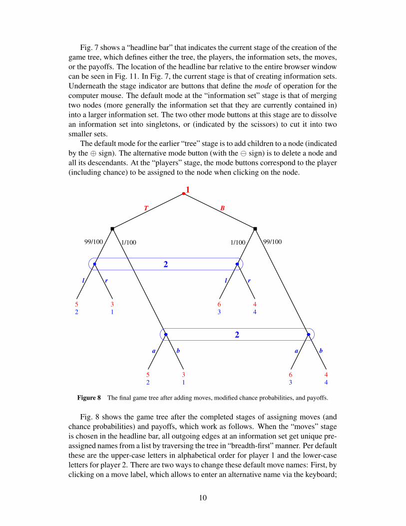
Fig. 7 shows a “headline bar” that indicates the current stage of the creation of thegame tree, which defines either the tree, the players, the information sets, the moves,or the payoffs. The location of the headline bar relative to the entire browser windowcan be seen in Fig. 11. In Fig. 7, the current stage is that of creating information sets.Underneath the stage indicator are buttons that define the mode of operation for thecomputer mouse. The default mode at the “information set” stage is that of mergingtwo nodes (more generally the information set that they are currently contained in)into a larger information set. The two other mode buttons at this stage are to dissolvean information set into singletons, or (indicated by the scissors) to cut it into twosmaller sets.
The default mode for the earlier “tree” stage is to add children to a node (indicatedby the ⊕ sign). The alternative mode button (with the sign) is to delete a node andall its descendants. At the “players” stage, the mode buttons correspond to the player(including chance) to be assigned to the node when clicking on the node.
b
99/100
3
a
l
1
2
4
r
1/100
3 6
431
a
1
3
2
rl
T
4
1/100
5
b
4
2
5
2
6
99/100
B
Figure 8 The final game tree after adding moves, modified chance probabilities, and payoffs.
Fig. 8 shows the game tree after the completed stages of assigning moves (andchance probabilities) and payoffs, which work as follows. When the “moves” stageis chosen in the headline bar, all outgoing edges at an information set get unique pre-assigned names from a list by traversing the tree in “breadth-first” manner. Per defaultthese are the upper-case letters in alphabetical order for player 1 and the lower-caseletters for player 2. There are two ways to change these default move names: First, byclicking on a move label, which allows to enter an alternative name via the keyboard;
10

this is not restricted to a single letter and need not be unique. On the left in Fig. 9, thisis shown for the chance probability of the right chance move which is changed from1/2 to 0.99 (which could also be entered as 99/100). The remaining probability forthe other chance move is automatically set to 0.01 so that the probabilities sum toone. A second, quick way to change all move names is the mode button below the“players” stage in the headline bar where all move names for a player are entered atonce, or altered from the displayed current list; this is shown in the right picture ofFig. 9 for player 2 whose default moves a,b,c,d are changed to l,r,a,b.
Figure 9 Changing move names, either by clicking on a single move name or chance probability(left), or by changing all moves of a player at once (right).
At the final “payoffs” stage, the leaves of the tree get payoffs to the two players,which are at first consecutively given as 0,1,2, . . . in order to have a unique payoff toidentify each leaf. As shown in Fig. 10, a player’s payoffs can then be changed at onceby replacing them with the intended payoffs for the game, where the numbering helpsto identify the leaves. Payoffs can also be changed individually. In addition, payoffscan be generated randomly. A zero-sum option can be chosen which automaticallysets the other player’s payoff to the negative of the payoff to the current player.
Figure 10 Changing all payoffs of player 1 from the pre-set values 0 1 2 3 4 5 6 7 (for easy identifi-cation) to their intended values.
The game tree is stored as its logical structure. Its graphical layout is generatedautomatically. Its parameters can be changed, such as the orientation of the gametree, which can grow vertically or horizontally in either direction, the default being
11

top-down. Fig. 11 shows a change of settings so that the game tree grows from left toright. Other parameters such as the colors used for the players, line thickness, fonts,and other dimensions can also be changed.
Figure 11 Changing the graphics settings, in this case to a left-to-right tree orientation and a Hel-vetica font.
Fig. 11 also shows the general layout of the graphical interface in the web browser.The top left offers file manipulation functions such as starting a new game, storingand loading the current game (together with its settings), and exporting it to a pictureformat (.png) and a scalable graphics format (.fig) that can be further manipulatedwith the xfig drawing program and converted to .pdf or .eps files for inclusion indocuments. On the top right various solution algorithms can be selected and started,and at the very right zoom operations and change of settings can be selected.
4
la
4.98
1.99
ra
3
1.01
4.02 5.98
B
lb
5 3
4
6
3.02
2
3.99 3.01
2
rb1
T
1
Figure 12 Strategic form of the game in Fig. 8.
The game in Fig. 8 has an interesting equilibrium structure. It is due to Bag-well (1995) and represents the commitment game shown earlier in Fig. 3, but wherethe commitment of player 1 is imperfectly observed due to some transmission noise:Namely, with a small probability (here 0.01), the second player observes the commit-ment incorrectly as the opposite move, which is represented by the chance moves and
12

the two information sets of player 2. The resulting strategic form is shown in Fig. 12.Finding all equilibria with GTE gives the following output, with three equilibria thatare isolated, each in a separate component.
Strategic form:
2 x 4 Payoff player 1
la lb ra rb
T 5 249/50 151/50 3
B 6 201/50 299/50 4
2 x 4 Payoff player 2
la lb ra rb
T 2 199/100 101/100 1
B 3 399/100 301/100 4
EE = Extreme Equilibrium, EP = Expected Payoffs
Rational:
EE 1 P1: (1) 1/100 99/100 EP= 393/98 P2: (1) 0 25/49 0 24/49 EP= 397/100
EE 2 P1: (2) 0 1 EP= 4 P2: (2) 0 0 0 1 EP= 4
EE 3 P1: (3) 99/100 1/100 EP= 489/98 P2: (3) 24/49 25/49 0 0 EP= 201/100
Decimal:
EE 1 P1: (1) 0.01 0.99 EP= 4.0102 P2: (1) 0 0.5102 0 0.4898 EP= 3.97
EE 2 P1: (2) 0 1.0 EP= 4.0 P2: (2) 0 0 0 1.0 EP= 4.0
EE 3 P1: (3) 0.99 0.01 EP= 4.9898 P2: (3) 0.4898 0.5102 0 0 EP= 2.01
Connected component 1:
{1} x {1}
Connected component 2:
{2} x {2}
Connected component 3:
{3} x {3}
In particular, the original SPE (T, lb) of the commitment game with perfect ob-servation and payoffs 5 and 2 has disappeared. Because the game does not have anynontrivial subgames (which are subtrees where each player knows that they are inthe subgame), the concepts of subgame perfection and backward induction no longerapply in the game with imperfectly observable commitment in Fig. 8. The reasonwhy (T, lb) is no longer an equilibrium is the following. Because player 1 commitsto move T with certainty, player 2 should choose move l when seeing T , because thisgives her a higher payoff than r. However, when player 2 sees move B of player 1, itmust be due to an error in the observation and player 2 would therefore also choosea rather than b; in short, la and not lb is a best response to T . However, (T, la) isnot an equilibrium either because against lb player 1 would choose B; in a sense,player 1 would exploit the fact that player 2 interprets B as an erroneous signal. This,however, seems to imply that player 1 has lost his commitment power due to the noisein the observation.
13

A Bagwell (1995) pointed out, and as is shown in the above list of equilibria, thisloss of commitment power only applies when the players are restricted to use purestrategies. There is in fact a mixed equilibrium, listed as the component {3} x {3} ,which has payoffs 489/98 and 201/100 to the two players that are close to the“Stackelberg” payoffs 5 and 2 when no noise is present. Here player 1 himself adds asmall amount of noise to the commitment and plays T and B with probabilities 0.99and 0.01. In turn, player 2 mixes between la and lb with probabilities 24/49 and25/49. That is, player 2 chooses l with certainty and is indifferent between a and bbecause when she sees move B, this signal may equally likely be received due to thechance move or due to player 1’s randomization. The mixture between a and b issuch that player 1 in turn is indifferent between T and B. The game also has the purestrategy equilibrium (B,rb) as before, listed as {2} x {2} with payoffs 4 and 4,and another mixed equilibrium {1} x {1} with similar payoffs.
With GTE, the game in Fig. 8 is created in a few minutes, and the equilibria arecomputed instantly. The game does not allow abstract parameters, such as ε for theerror probability as in the analysis by Bagwell (1995), which is here chosen as 0.01.However, as a quick way to test a typical case of this game-theoretic model, GTE isa valuable tool.
4 Examples of analyzing games in strategic form
In this section we give examples of strategic-form games analyzed with GTE. Thesealso demonstrate the use of GTE as a research tool for game theory, for questions onthe possible number of equilibria, or the description of equilibrium components inthe context of strategic stability.
Figure 13 GTE input of a 6×6 game in strategic form.
Fig. 13 shows the input of a game in strategic form, currently implemented for twoplayers only. For each player one needs to specify the number of strategies, whichare the rows for player 1 and columns for player 2, and a payoff matrix. Names forthe strategies are generated automatically as upper case letters for player 1 and lowercase letters for player 2, and can be changed. If the strategic form has been generated
14

from the extensive form, then the strategies are shown as tuples of moves, one foreach information set.
One can choose a zero-sum input mode where the payoffs to player 2 are auto-matically the negative of the payoffs to player 1. Similarly, one can input a symmetricgame where the square payoff matrices to player 1 and 2 are a matrix A and its trans-pose A>; the game is symmetric because it does not change when the players areexchanged. In both cases, only the payoff matrix of player 1 is entered.
Payoffs can be entered as integers, fractions, or with a decimal point where thedisplay can be switched between fractions and decimals; internally they are all storedas fractions. The “Align and Update” button aligns the entries in columns and updatesthe second player’s payoffs for zero-sum and symmetric games.
The input of bimatrix games and the computation of their equilibria has the func-tionality of the popular webpage of Savani (2005) which has been used tens of thou-sands of times. The extra feature in GTE is the graphical output as in Fig. 12, forexample, which is accessed by the “Matrix Layout” tab shown at the top of Fig. 13.
The game in Fig. 13 has 75 equilibria, listed as follows; the output displays eachequilibrium in a single line, which we have here broken into two lines, one per player,to fit the page.
EE 1 P1: (1) 1/30 1/6 3/10 3/10 1/6 1/30 EP= 3/2
P2: (1) 1/6 1/30 3/10 3/10 1/30 1/6 EP= 3/2
EE 2 P1: (2) 0 0 1/33 5/33 4/11 5/11 EP= 24/11
P2: (2) 0 0 5/33 1/33 5/11 4/11 EP= 24/11
EE 3 P1: (3) 1/128 0 0 7/64 47/128 33/64 EP= 12/7
P2: (3) 0 0 5/21 13/189 59/189 8/21 EP= 297/128
...
EE 74 P1: (74) 0 0 13/32 0 0 19/32 EP= 450/103
P2: (74) 33/103 70/103 0 0 0 0 EP= 477/16
EE 75 P1: (75) 0 0 0 0 1 0 EP= 270
P2: (75) 1 0 0 0 0 0 EP= 270
Connected component 1:
{1} x {1}
...
Connected component 75:
{75} x {75}
This game is the smallest known example that refutes a conjecture by Quint andShubik (1995) that an n×n game has at most 2n−1 equilibrium components, here forn = 6. It has been constructed by von Stengel (1999) using methods from polytopetheory, with the specific small integers in Fig. 13 described by Savani and von Stengel(2004, p. 25). Studying games with large numbers of equilibria is obviously greatlyaided by computational tools; for another example see von Stengel (2012).
Fig. 14 shows at the top left a symmetric “anti-coordination” game where the onlynonzero payoffs are −1 to both players on the diagonal. Because no payoff is posi-tive, any cell with payoff zero to both players is an equilibrium, and these equilibriaare connected by line segments to form a “ring” that defines the topologically con-nected component 2 as in the output shown on the right in Fig. 14. The game also hasan isolated completely mixed equilibrium shown as component 1. Interestingly, only
15

−1
A
0B
−1
0
0
1 b
−1
−1
−1
0
0
0
c
0
0 0
0
−1
a
0
2
0
C
−1
A
0.1B
−1
0.1
0
1 b
−1
−1
−1
0.1
0
0.1
c
0
0.1 0
0
−1
a
0.1
2
0
C
EE 1 P1: (1) 1/3 1/3 1/3 EP= -1/3 P2: (1) 1/3 1/3 1/3 EP= -1/3
EE 2 P1: (2) 1 0 0 EP= 0 P2: (2) 0 1 0 EP= 0
EE 3 P1: (2) 1 0 0 EP= 0 P2: (3) 0 0 1 EP= 0
EE 4 P1: (3) 0 1 0 EP= 0 P2: (3) 0 0 1 EP= 0
EE 5 P1: (3) 0 1 0 EP= 0 P2: (4) 1 0 0 EP= 0
EE 6 P1: (4) 0 0 1 EP= 0 P2: (4) 1 0 0 EP= 0
EE 7 P1: (4) 0 0 1 EP= 0 P2: (2) 0 1 0 EP= 0
Connected component 1:
{1} x {1}
Connected component 2:
{2, 4} x {2}
{3, 4} x {4}
{4} x {2, 4}
{2, 3} x {3}
{3} x {3, 4}
{2} x {2, 3}
----------------------------------------------------------------
EE 1 P1: (1) 1/3 1/3 1/3 EP= -3/10 P2: (1) 1/3 1/3 1/3 EP= -3/10
Connected component 1:
{1} x {1}
Figure 14 Top left: 3×3 game which has two equilibrium components, shown on the right. Bottomleft: The same game but with perturbed payoffs so that only component 1 remains (see bottom right).
component 1 is strategically stable in the sense that there is always an equilibriumnearby when the payoffs are slightly perturbed. In the game shown at the bottom left,the payoffs are perturbed so that the only equilibrium that remains is the completelymixed equilibrium in component 1; the perturbations from zero to 0.1 can be changedto independent arbitrarily small positive reals with the same effect.
0
A
0B
0
0
−2
1 b
0
0
−1
0
0
0
c
−2
0 0
0
−1
a
0
2
0
C
EE 1 P1: (1) 0 1 0 EP= 0 P2: (1) 0 1 0 EP= 0
EE 2 P1: (1) 0 1 0 EP= 0 P2: (2) 0 0 1 EP= 0
EE 3 P1: (2) 1 0 0 EP= 0 P2: (3) 1 0 0 EP= 0
EE 4 P1: (2) 1 0 0 EP= 0 P2: (2) 0 0 1 EP= 0
EE 5 P1: (3) 0 0 1 EP= 0 P2: (3) 1 0 0 EP= 0
EE 6 P1: (3) 0 0 1 EP= 0 P2: (1) 0 1 0 EP= 0
Connected component 1:
{1, 3} x {1}
{2, 3} x {3}
{3} x {1, 3}
{1, 2} x {2}
{2} x {2, 3}
{1} x {1, 2}
Figure 15 3×3 game which has only a “ring” of equilibria as its sole stable component, shown onthe right.
The concept of strategic stability is due to Kohlberg and Mertens (1986). Fig. 15shows a game that is also symmetric like that at the top left of Fig. 14 (the symmetryis easy to see due to the staggered payoffs in the lower left and upper right of eachcell). It is strategically equivalent (by subtracting constants from columns of therow player’s payoffs and from rows of the column player’s payoffs) to the game ofKohlberg and Mertens (1986, p. 1034) and has a “ring” consisting of line segmentsas its only equilibrium component. As Kohlberg and Mertens have shown, any point
16

on that ring can be chosen so that a suitably perturbed game has its only equilibriumnear that point, which can be verified by experimenting with numeric perturbationsof the game. Correspondingly, the entire ring defines the minimal stable componentof the game.
8
A
3B
−1
−2
0
1 b
D0 0
5
4
0
1
a
0
2
0
2
c
−23
−15
−1
0
−21
3
−11
0
2
1
C
EE 1 P1: (1) 0 0 0 1 EP= 0 P2: (1) 31/282 5/141 241/282 EP= 0
EE 2 P1: (1) 0 0 0 1 EP= 0 P2: (2) 0 3/4 1/4 EP= 0
EE 3 P1: (1) 0 0 0 1 EP= 0 P2: (3) 0 1 0 EP= 0
EE 4 P1: (1) 0 0 0 1 EP= 0 P2: (4) 3/4 1/4 0 EP= 0
EE 5 P1: (1) 0 0 0 1 EP= 0 P2: (5) 1/2 0 1/2 EP= 0
EE 6 P1: (1) 0 0 0 1 EP= 0 P2: (6) 11/16 0 5/16 EP= 0
EE 7 P1: (2) 1 0 0 0 EP= 5 P2: (7) 1 0 0 EP= 4
Connected component 1:
{1} x {1, 2, 3, 4, 5, 6}
Connected component 2:
{2} x {7}
c
a b
Figure 16 Left: 4×3 game with two equilibrium components, shown on the right. In component 1,player 1 plays D and player 2 plays so that player 1 gets at most payoff 0, shown by the hexagon at thebottom right (see also Hauk and Hurkens, 2002, Fig. 4). Component 2 is the pure-strategy equilibrium(A,a).
Fig. 16 shows another game related to strategic stability, due to Hauk and Hurkens(2002, p. 74). This game corresponds to an extensive game where player 1 can firstchoose between an “outside option” D with constant payoff zero to both players orelse play in a 3×3 simultaneous game. The game has two equilibrium components,the pure equilibrium (A,a) and the outside option component where player 2 ran-domizes in such a way that player 1 gets at most payoff zero and therefore will notdeviate from D.
Interestingly, the larger component in this game has the property that it has indexzero but is nevertheless strategically stable, that is, any perturbed game has equilibrianear that component, as shown by Hauk and Hurkens (2002). The larger componentin the game in Fig. 14 has also index zero and is not stable, which is what one wouldnormally expect. The index is a certain integer defined for an equilibrium component,with the important property that the sum over all equilibrium indices is one, and thatfor generic perturbations each equilibrium has index 1 or −1, which is always 1 for apure-strategy equilibrium (see Shapley, 1974). A symbolic computation of the indexof an equilibrium component for a bimatrix game is described by Balthasar (2009,Chapter 2). Its implementation is planned as a future additional feature of GTE.
All currently implemented algorithms of GTE apply only to two-player games. Asimple next stage is to allow three or more players at least for the purpose of drawinggames and generating their strategic form. Algorithms for finding all equilibria of agame with any number of players using polynomial algebra are described by Datta(2010); some of these require computer algebra packages, so far not part of GTE.
17

5 Equilibrium computation for games in strategic form
In this section, we describe the algorithm used in GTE that finds all equilibria of atwo-player game in strategic form. This algorithm searches the vertices of certainpolyhedra defined by the payoff matrices, which is practical for up to about 20 strate-gies per player. For larger games, one can normally still find in reasonable time oneequilibrium, or possibly several equilibria with varying starting points, using the path-following algorithms by Lemke and Howson (1964) and Lemke (1965) mentioned atthe end of this section. We assume some familiarity with pivoting as used in thesimplex algorithm for linear programming, which in the present context is explainedfurther in Avis et al. (2010).
The best response condition describes, in a general finite game in strategic form,when a profile of mixed strategies is a Nash equilibrium. If player 1, say, has mpure strategies, then his set X of mixed strategies is the set of probability vectorsx = (x1, . . . ,xm) so that xi ≥ 0 and ∑
mi=1 xi = 1. Geometrically, X is a simplex which
is the convex hull of the m unit vectors in Rm . If x is part of a Nash equilibrium, then xhas to be a best response against the strategies of the other players. The best responsecondition states that this is the case if and only if every pure strategy i so that xi > 0 issuch a best response (the condition is easy to see and was used by Nash, 1951). Thisis a finite condition, which requires to compute player 1’s expected payoff for eachpure strategy i, and to check if the strategies i in the support {i | xi > 0} of x giveindeed maximal payoff. These maximal payoffs have to be equal, and the resultingequations typically determine the probabilities of the mixed strategies of the otherplayers.
3
2
r
0
T
1
2
1
2
B
l
0
1
2
3
1T
l
B0
1
3
r
2
0
2EE 1 P1: (1) 1 0 EP= 1 P2: (1) 1 0 EP= 3
EE 2 P1: (1) 1 0 EP= 1 P2: (2) 1/2 1/2 EP= 3
EE 3 P1: (2) 0 1 EP= 2 P2: (3) 0 1 EP= 2
Connected component 1:
{1} x {1, 2}
Connected component 2:
{2} x {3}
Figure 17 A “threat game” in extensive form, its 2× 2 strategic form, and its equilibrium compo-nents.
For two players, these constraints define “best response polyhedra” that simplifythe search for equilibria. We illustrate this geometric apprach with an example; fora general exposition and detailed references see von Stengel (2002; 2007). Fig. 17shows a simple game tree which has the SPE (B,r), and another equilibrium compo-nent where player 2 “threatens” to choose l with probability at least 1/2 and player 1chooses T .
Fig. 18 shows on the left the mixed strategy y of player 2, which is defined by theprobability that she chooses move r, say, together with the expected payoff to player 1for his two pure strategies T and B. These expected payoffs are linear functions ofy (because the game has only two players; for more than two players, the expected
18

r
l
payoff player 2
B
T
prob( )
payoff player 1
2
11/20
1
2
00
1rprob( )
1
0
3
B
Figure 18 Expected payoffs to the two players in the threat game in Fig. 17 as a function of themixed strategy of the other player.
payoff for a pure strategy of player 1 is a product of mixed strategy probabilities ofthe other players, which is no longer linear). The right picture shows the expectedpayoffs for the pure strategies l and r of player 2 as a function of the mixed strategyof player 1.
These pictures show when a pure strategy is a best response against a mixedstrategy of the other player: T is a best response of player 1 when prob(r) ≤ 1/2,and B is a best response when prob(r)≥ 1/2. Strategy r of player 2 is always a bestresponse, and l is a best response when prob(B) = 0.
B
lrT
r
lB
T
prob( )11/20 0 1
rprob( ) B0
1
2 2
1
0
3QP
u v
y x
Figure 19 The polyhedra Q and P in (1) that define the “upper envelope” of the payoffs in Fig. 18,with additional circled facet labels for unplayed strategies, and equilibrium strategy pairs.
In Fig. 19, the same pictures are shown more abstractly where u and v are theexpected payoffs to player 1 and 2, respectively, which are required to be at leastas large as the expected payoff for every pure strategy. In a general m× n bimatrixgame, let ai j and bi j be the payoffs to player 1 and 2, respectively, for each purestrategy pair i, j. Analogous to X , let Y be the mixed strategy simplex of player 2given by Y = {y ∈ Rn | y j ≥ 0, ∑
nj=1 y j = 1}. Then P and Q are the best response
polyhedra
P = {(x,v) ∈ X×R | ∑mi=1 bi jxi ≤ v, 1≤ j ≤ n},
Q = {(y,u) ∈ Y ×R | ∑nj=1 ai jy j ≤ u, 1≤ i≤ m}. (1)
In Fig. 19, Q is shown on the left and refers to the set of mixed strategies y of player 2together with the best responses of player 1 and corresponding payoff u to player 1.
19

Consider one of the inequalities ∑nj=1 ai jy j ≤ u in the definition of Q for some pure
strategy i of player 1, which in the example is either T or B. When this inequalityis tight, that is, holds as equality, then i is clearly a best response to y. This tightinequality defines a face (intersection with a valid hyperplane) of the polyhedron, andis often a facet (a face of maximum dimension), as here for both strategies T and B;however, for the polyhedron P on the right in Fig. 19 the tight inequality ∑
mi=1 bi jxi =
v when j is the pure strategy l of player 2 does not define a facet because it only holdsfor the single point where prob(B) = 0 and v = 3, that is, for (x,v) = ((1,0),3) ∈ P.
We label each point (y,u) of Q with the strategy i of player 1 whenever i is a bestresponse to y, that is, when ∑
nj=1 ai jy j = u. In addition, (y,u) is labeled with strategy
j of player 2 if y j = 0. The labels for these unplayed pure strategies are shown withcircles around them in Fig. 19. So any point ((1,0),u) where prob(r) = 0 (the leftedge of Q) is labeled with r, and any point ((0,1),u) where prob(r) = 1 and henceprob(l) = 0 (the right edge of Q) is labeled with l . Similarly, in the right picture theleft and right edges of P have label B and T , respectively. The bottom edge of P islabeled with the pure strategy r, and the left vertex (x,v) = ((1,0),3) has label l inaddition to the labels B and r.
With this labeling, an equilibrium (x,y) of the game with payoffs u and v to player1 and 2 is given by a pair ((x,v),(y,u)) in P×Q that is completely labeled, that is,each pure strategy, here T,B, l,r, of either player appears as a label of (x,v) or (y,u).Otherwise, a missing label represents a pure strategy that has positive probability butis not a best response, which does not hold in an equilibrium because it contradictsthe best response condition.
In Fig. 19, one equilibrium (x,y), indicated by the small disks to mark the twopoints (x,v) and (y,u), is given by x = y = (0,1) with u = v = 2, which is the purestrategy pair (B,r). Here the point (y,u) of Q has labels B and l and the point (x,v)of P has labels r and T , so these two points together have all labels T,B, l,r. A secondequilibrium component, indicated by the rectangles, is given by any point (y,u) onthe entire edge of Q that has label T and (x,v) = ((1,0),3) in P which has the threelabels r, l,B. These are also the two equilibrium components in the GTE output inFig. 17. The edge of Q with label T is the convex hull of the two vertices ((1,0),1)with labels T and r, and ((1/2,1/2),1) with labels T and B. Each of these verticesof Q, together with the vertex ((1,0),3) of P, forms a completely labeled vertex pair.For these two vertex pairs of P×Q, one label (r or B) appears twice and represents abest-response pure strategy that is played with probability zero, which is allowed inequilibrium.
The extreme equilibria computed by GTE are in fact all vertex pairs of P×Qthat are completely labeled, which are then further processed so as to detect the equi-librium components. We give an outline of how these computations work in GTE,described in detail and compared with other approaches by Avis et al. (2010).
Vertex enumeration, that is, listing all vertices of a polyhedron defined by linearinequalities, is a well-studied problem where we use the lexicographic reverse searchmethod lrs by Avis (2000; 2006). This method reverses the steps of the simplexalgorithm for linear programming for a certain deterministic pivoting rule. It startswith a vertex v0 of the polyhedron and a linear objective function that is maximized
20

at that vertex. The simplex algorithm for maximizing this linear function computesfrom every vertex a path of pivoting steps to v0 . With a deterministic pivoting rule,that path is unique. In lrs, the pivoting rule chooses as entering variable the variablewith the least index (i.e., smallest subscript) that improves the objective function, andthe leaving variable via a lexicographic rule. The unique paths of simplex steps fromthe vertices to v0 define a tree with root v0 . The lrs algorithm explores this tree bytraversing the tree edges in the reverse direction using a depth-first search.
In lrs, as in the simplex algorithm, the vertices of P×Q are represented by basicfeasible solutions to the inequalities in (1) when they are represented in equality formvia slack variables. Here, these are vectors s in Rn and r in Rm so that the constraintsthat define P and Q are written as
m
∑i=1
bi jxi + s j = v, ri +n
∑j=1
ai jy j = u, xi,s j,ri,y j ≥ 0 (2)
for 1 ≤ i ≤ m, 1 ≤ j ≤ n, and ∑ni=1 xi = 1 and ∑
nj=1 y j = 1 so that x ∈ X and y ∈ Y .
A feasible solution x,s,v,r,y,u to (2) defines a point in P×Q and vice versa. A tightinequality corresponds to a slack variable that is zero. In fact, the labels for a strategypair x,y, where u and v are chosen minimally so that (2) holds, which determines rand s, are the pure strategies i so that xi = 0 or ri = 0 for player 1 and y j = 0 or s j = 0for player 2. The equilibrium condition of being completely labeled is equivalent tothe complementarity condition
xi ri = 0 (1≤ i≤ m), y j s j = 0 (1≤ j ≤ n). (3)
In a basic feasible solution to (2), the labels correspond to the indices i or j of thenonbasic variables, and to basic variables that happen to have value zero.
Basic solutions where basic variables have value zero are called degenerate, andgames where this happens are also called degenerate. It is easy to see (see von Sten-gel, 2002) that this corresponds to a mixed strategy of a player that has more bestresponses than the size of its support; in terms of labels, this defines a point of Pwith more than m labels or a point of Q with more than n labels. An example isthe degenerate game in Fig. 17 where the pure strategy T (which is a mixed strat-egy x = (1,0) with a support of size one) has two best responses, which is the point((1,0),3) of P in Fig. 19 with three labels B, l,r. For extensive games, the strategicform is typically degenerate, as the examples in Fig. 3 and 17 demonstrate. In lrs,all arithmetic computations are done in arbitrary precision arithmetic (rather thanfloating point arithmetic with possible rounding errors) in order to recognize withcertainty that a basic variable is zero. In addition, lrs uses the economical integerpivoting method where basic feasible solutions are represented with integers ratherthan rational numbers; see, for example, von Stengel (2007, Section 3.5).
After enumerating all vertices of P and Q with lrs, those pairs that fulfill thecomplementarity condition (3) are the extreme equilibria of the game. Avis et al.(2010) also describe an improved method lrsNash, which is used in GTE, where onlythe vertices of one polytope, say P, are generated, and the set L of labels missingfrom each such vertex (x,v) is used to identify the face Q(L) of the other polytopethat has exactly the labels in L. If this face is not empty, then each of its vertices
21
(y,u) defines an extreme equilibrium (x,y). An alternative method to enumerate allextreme equilibria is the EEE method of Audet et al. (2001) which performs a depth-first search that chooses one tight inequality for either player in each search step. InAvis et al. (2010), EEE is implemented with exact integer arithmetic and comparedwith lrsNash, and performs better for larger games from size 15×15 onwards.
Given the list of extreme equilibria, the set of all equilibria is completely de-scribed as follows (for details see Avis et al., 2010). Consider the bipartite graphR with edges (x,y) that are the extreme equilibria. Each connected component Cof this graph defines a topologically connected component of equilibria, as it is out-put by GTE. For each C, identify the maximal bipartite “cliques” in R of the formU ×V ⊆ C, that is, every pair (x,y) in U ×V is an extreme equilibrium. Then anyconvex combination of U paired with any convex combination of V is also a Nashequilibrium, and every equilibrium of the game can be represented in this way. Theremay be several such cliques that define a component C, as in Fig. 14 and 15 above.In GTE, the maximal cliques U×V are computed with an extension of the fast cliqueenumeration algorithm by Bron and Kerbosch (1973).
For a two-player game in strategic form, GTE computes by default all Nash equi-libria, as just described. However, the state-of-the-art algorithms lrsNash and EEEhave exponential running time due the typically exponential growth of the numberof vertices of P×Q. These equilibrium enumeration algorithms therefore take pro-hibitively long for games with more than 25, certainly 30 pure strategies for eachplayer. In addition, it is NP-hard to decide if a bimatrix game has more than oneNash equilibrium (Gilboa and Zemel, 1989; Conitzer and Sandholm, 2008), so onecannot expect to answer that question quickly for larger games.
In practice, a finite game may represent a discretization of an infinite game, whereit may be useful to know its equilibria when each player has several hundred strate-gies. In that case, it is still possible to use methods that find one equilibrium, suchas the classic algorithm by Lemke and Howson (1964). This is a path-following al-gorithm that follows a sequence of pivoting steps, similar to the simplex algorithmfor linear programming (for expositions see Shapley, 1974, or von Stengel, 2002;2007). Like the simplex algorithm, it can take exponentially many steps on certainworst-case instances (Savani and von Stengel, 2006). However, these seem to be rarein practice, and the algorithm is typically fast for random games.
The Lemke–Howson algorithm has a free parameter, which is a pure strategy ofa player that together with the best response to that strategy defines a “starting point”of the algorithm in the space of mixed strategies X ×Y . Varying this starting pointover all pure strategies may lead to different equilibria (however, if that is not thecase, the game may still have equilibria that are elusive to the algorithm).
GTE uses a related but different method that is implemented using the algorithmby Lemke (1965), which allows for starting points that can be arbitrary mixed strategypairs (x,y) (von Stengel, van den Elzen, and Talman, 2002). In addition, the compu-tation can be interpreted as the “tracing procedure” by Harsanyi and Selten (1988),where players’ strategies are best responses to a weighted combination of their prior(x,y) and the actual strategies that they are playing. Initially, the players only react tothe prior, whose weight is then decreased; equilibrium is reached when the weight of
22

the prior becomes zero. If starting from sufficiently many random priors gives alwaysthe same equilibrium, this does not prove that this equilibrium is unique, but may beconsidered as sufficient reason to suggest this as a plausible way to play the game.
The computational experiments of von Stengel, van den Elzen, and Talman (2002)show that for random games, the method finds an equilibrium in a small numberof pivoting steps, and that typically many equilibria are found by varying the priorby choosing it uniformly at random from the strategy simplices. For a systematicinvestigation of this method in GTE, it would be useful to generate larger games asdiscretizations of games defined by arithmetic formulas for payoff functions; this isa future programming project where a closer integration with Gambit is envisaged.
6 Equilibrium computation for games in extensive form
The standard approach to finding equilibria of an extensive game is to convert it tostrategic form, and to apply the corresponding algorithms. However, the number ofpure strategies grows typically exponentially in the size of the game tree. In contrast,the sequence form is a strategic description that has the same size as the game tree,which is used in GTE. We sketch the main ideas here; for more details see vonStengel (1996; 2002) or von Stengel, van den Elzen, and Talman (2002).
7
c
2
E
0
1
6
f
8
1
D
26
F
2
8
4e
C
5 3
2
g
7
2
8
h
2
A
2
b
B
1
d
4
2
7
3
2
E F
a
Figure 20 Extensive game with perfect information for player 2 and no information for player 1.
Fig. 20 shows an extensive game where player 1 has four moves at the root andtwo moves at his second information set. Player 2 has perfect information and foursingleton information sets with two moves each. A pure strategy of a player defines amove for every information set, so player 1 has 8 and player 2 has 16 pure strategies.Some of these pure strategies can be identified because they describe the same “plan”of playing the game. A reduced pure strategy does not specify a move at an infor-mation set that is unreached due to an earlier own move of the player. For example,after move a player 2 does not need to specify move g or h because the informationset with that move cannot be reached. We represent such an unspecified move byan asterisk “ * ” at the place where the move would be listed, so a*ce is a reducedstrategy where * stands for either g or h, as in the strategy bgce where no reduction
23

is possible. The reduced strategic form is shown in Fig. 21, which is a 5×12 game.Each cell shows the payoffs that result when the two strategies meet.
2
5
6
3
3
4
22
6
3
6 6
0
7
7
1
7
2
4
1
7
4
2
2
8
6
4
2
2
1
7
3
7
2
2
8
7
4
7
4
2
CE
4
4
2
bgce
0
8
4
3
1
7
bhcf
6
8
7
7
6
a*df
2
a*ce
2 8
6
bgdf
6
3
bhce bhde
2
2
7
8
2
2A*
4
8
3
2
78
bgde
6
a*de
6D*
6
2
6
7
6
8
3
3
7
2
6
6
0
4
CF
6
a*cf
8
4
B*
8
8
8
2
4
2
2
4
1
bgcf
7
7
2
8
bhdf
0 5
3
3
4
2
4
2
7
6
3
8
8
5 5
4 4
Figure 21 Reduced strategic form of the game in Fig. 20. In a reduced strategy, any move at aninformation set that cannot be reached due to an earlier own move is left unspecified and replacedby “ * ”.
In this game, a mixed strategy requires four independent probabilities for player 1(the fifth is then determined because probabilities sum to one) and eleven for player 2.In general, the number of reduced strategies is exponential in the size of the game tree,so there is a large number of mixed strategy probabilities to compute.
2
47
18
2
2
CE
c
4
3
7
bh0/
6
f
5
2
A
e
6
bg
D
2
7
CF
a
8
B
8
2
0
d
3
1
Figure 22 Sequence form payoffs of the game in Fig. 20. All empty cells have zero entries. The rowsare played with a probability distribution, whereas the columns are played with weights yσ subject tothe equations y /0 = 1 = ya + ybg + ybh = yc + yd = ye + y f .
The sequence form is a compact strategic description of the game that has thesame size as the game tree. Instead of strategies, it uses sequences of moves of a givenplayer along a path from the root to a leaf. The payoff matrices are sparse and containpayoffs for those pairs of sequences of the two players that lead to a leaf, as shownin Fig. 22 for the game in Fig. 20. This table is evidently more compact, and vastlymore so for larger games. In this game, sequences and reduced strategies coincidefor player 1, because that player does not get any information about the moves ofthe other player. For player 2, her sequences σ are played with probabilities yσ thatare not distributions over the set of all sequences, but are subject to three separateequations ya + ybg + ybh = 1, yc + yd = 1, ye + y f = 1. These equations express
24

the revealed information to player 2 following the respective moves A, B, and C ofplayer 1, and can be derived systematically from the structure of the information sets(with one equation per information set, where we have substituted some equationssuch as yb = ybg+ybh for the unused nonterminal sequence b; also, player 2’s emptysequence /0 leads here to the rightmost leaf and has constant probability y /0 = 1).
The twelve reduced strategies of player 2 are in effect the combinations of one ofthe sequences a,bg,bh combined with one of c,d and one of e, f , respectively. In thesequence form, these sequences are randomized independently. This randomizationtranslates to a behavior strategy, where the player randomizes locally over his movesat each information set rather than globally over his pure strategies as in a mixedstrategy. The underlying assumption about the information sets is that of perfectrecall which says that a player does not forget what he knew or did earlier. Using thesequence form implies the theorem of Kuhn (1953) that a player with perfect recallcan replace a mixed strategy by an equivalent behavior strategy.
In GTE, the sequence form is implemented with the path-following algorithmof Lemke (1965) mentioned at the end of the previous section, as described by vonStengel, van den Elzen, and Talman (2002), which starts from an arbitrary “prior”as a starting vector and finds one equilibrium. It can be applied to relatively largeextensive games where the strategic form is hopelessly large to be used. For smallerextensive games, an enumeration of all Nash equilibria based on the sequence formis implemented as described by Huang (2011, Chapter 2); for a related approach seeAudet, Belhaiza, and Hansen (2009). The number of independent probabilities inthe sequence form is at most that number in the reduced strategic form. For exam-ple, player 2 in Fig. 22 has four such independent probabilities, like ya,ybg,yc,ye , asopposed to eleven for her reduced strategies; player 1 has four independent proba-bilities for both sequences and reduced strategies. Huang’s approach only uses theseindependent probabilities and thus keeps a low dimension of the suitably definedbest-response polyhedra, which is important for the employed vertex enumerationalgorithms that have exponential running time.
7 Software architecture and development
In this final section, we describe the architecture of the GTE software on the serverand client computers, and its development. The GTE program is open-source and partof the Gambit project, with the goal of further integration with the existing Gambitmodules. The development is time intensive and relies on the efforts of volunteers,where we strongly invite any interested programmer to contribute.
The GTE software is accessed by a web browser. Behind its web address runs aserver computer, which delivers a webpage and the game-drawing software of GTEto the user’s client computer. The user can then create games, and store them on hisclient computer. The game solvers for equilibrium computation reside on the server.They are invoked by sending a description of the game from the client to the serverover the internet. When the algorithm has terminated, the server sends the text withthe computed equilibria back to the client where they are displayed.
The client program with the graphical user interface (GUI) is written in a variantof the JavaScript programming language called ActionScript which is displayed with
25

the “Flash Player”. Flash is a common software that runs as a “plug-in” on mostweb browsers. We chose Flash for GTE in 2010 because of the predictability andspeed of its graphical display. However, Flash does not work on the iPad and iPhonemobile devices (it does work on regular Apple computers), with the more universallyaccepted HTML5 standard as its suggested replacement. In the future, we plan toreplace the ActionScript programs by regular JavaScript along with streamlining andfurther improving the GUI part of GTE.
For security reasons, the client program requires active permission of the userwhen writing or reading files on the client computer. When storing or loading a gameas a local file, this is anyhow initiated by the user and therefore causes no additionaldelay. We have designed a special XML format for games in extensive or strategicform, where XML stands for “extensible markup language” similar to the HTMLlanguage for web pages. The tree is described by its logical structure. For example,the leftmost leaf in Fig. 17 reached by move T is encoded as follows:
<outcome move="T">
<payoff player="1">1</payoff>
<payoff player="2">3</payoff>
</outcome>
In addition, the file contains parameters for graphical settings such as the orientationof the game tree. The files can be converted to and from the file format used byGambit. The XML description is also used to encode the game for sending it to theserver for running a game solver.
Communication with the server requires identifying the user when there are dif-ferent simultaneous client sessions, and the use of the relevant internet protocols.These are standard methods used for typical internet transactions, which we use asfreely available routines in the Java programming language in which we have writtenthe server programs.
The first version of GTE was written on a publically provided server (the GoogleApp engine). For security reasons, all programs on that platform have to be writtenin Java, and are restricted in their ability to access programs written in other pro-gramming languages, called “native” code. In particular, we could not use the Cprogram lrs for vertex enumeration, which was therefore rewritten in Java. However,this requires to duplicate in Java any improvement of lrs such as the lrsNash programmentioned in Section 5, which is inefficient and prone to errors. In addition, it isdifficult to incorporate other game solvers. For that reason, the web server for GTE isnow provided on a university computer, and uses the original lrs code of Avis (2006).
GTE allows to compute all Nash equilibria of a two-player game, but the runningtime increases exponentially with the size of the game. This means that there is arelatively narrow range of input size (currently about 15 to 20 strategies per player)where the efficiency of the implementation (such as a factor of ten in running time)matters, and beyond which the computation takes an impractically long time. Forsmall games, the game solvers would run satisfactorily on the client using JavaScript,although at present there are no good arbitrary precision arithmetic routines for thisprogramming language, apart from having to implement the algorithms separately.
26
For games of “medium” size (below the “exponential barrier”), it is best to use astate-of-the-art algorithm on the server, which works equally well for small games.
However, one problem is that computations of, say, one hour also use the com-putational resources of the server, which degrade its performance, and which will beslow if there are multiple such computations at the same time. Here, we provide theoption of installing the server on any local computer, which then also works inde-pendently of an internet connection. This requires downloading and compiling theGTE code, together with the necessary components of a Java compiler, a lightweightserver program called “Jetty” to communicate locally with the web browser, and the(free) software for compiling the ActionScript part of GTE into an executable Flashprogram. This requires time and patience, probably more so than an installation ofGambit, but offers the same interface as that known from the web, so that the usermay find the investment worth it.
All GTE software is open source and free to use and alter under the GNU Gen-eral Public Licence (which requires derived software to be free as well). The softwarerepository is at https://github.com/gambitproject/gte/wiki (including doc-umentation), as part of the Gambit project which has long been open-source. Theversion control system and collaborative tool “git” stores the current and all previousversions of the project. Git efficiently stores snapshots of the entire project with allmodules and documentation, which can be branched off and re-merged in decentral-ized development branches. The github repository for storing projects developedwith git is free to use for open-source software, and offers a convenient web interfacefor administration and documentation.
Open-source software is the appropriate way to develop an academic project suchas GTE which has limited commercial use. Academic software should be publicallyavailable for making computations reproducible, which is increasingly recognized asa need for validating scientific results that rely on computation (Barnes, 2010).
On the algorithm side, one of the next steps is to integrate other existing gamesolvers. Foremost among these are the algorithms already implemented in Gambit,which should be easily incorporated via their existing file formats for input and out-put. These include (see McKelvey, McLennan, and Turocy, 2010) algorithms forfinding Nash equilibria of more than two players with polynomial systems of equa-tions, or via iterated polymatrix approximation (Govindan and Wilson, 2004), or sim-plicial subdivision (van der Laan, Talman, and van der Heyden, 1987), and the recentimplementation of “action-graph games” (Jiang, Leyton-Brown, and Bhat, 2011).Moreover, larger games should not be created manually but automatically. One focusof the current development of Gambit is to provide better facilities for the automaticgeneration of games using the Python programming language.
So far, the focus of GTE development has been to design a robust and attractivegraphical “front end” for creating and manipulating games. Such an implementationdoes not count as scholarly research, so it is difficult to fund it directly with a researchgrant, or to let a PhD student invest a lot of time in it. As a topic for an MSc thesisor undergraduate programming project, usually too much time is needed to becomefamiliar with the existing code or the necessary background in game theory. TheGambit project and GTE were sponsored by studentships from the “Google Sum-
27

mer of Code” in 2011 and 2012. Here, the most successful projects for GTE werethose where the students could bring in their technical expertise on web graphics, forexample, to complement our background in game-theoretic algorithms.
As with open-source software in general, the development of GTE relies on theefforts, competence, and enthusiasm of volunteers, where we were lucky to get helpfrom excellent students listed in the Acknowledgments. We invite and encourage anyinterested programmer to contribute to this project.
Acknowledgments We are indebted to Mark Egesdal, Alfonso Gomez-Jordana and Martin Prausefor their invaluable contributions as programmers of GTE. Mark Egesdal designed the main programstructure and coined the name “Game Theory Explorer”, with financial support from a STICERDresearch grant at the London School of Economics in 2010. Alfonso Gomez-Jordana and MartinPrause were funded by the Google Summer of Code in 2011 and 2012 for the open-source Gambitproject, and continue as contributing volunteers. Karen Bletzer wrote conversion programs betweenGTE and Gambit file formats. Wan Huang implemented the enumeration of Nash equilibria basedon the sequence form. We thank Theodore L. Turocy for inspiring discussions and for his support ofGTE as part of Gambit. David Avis has written the lrsNash code for computing all Nash equilibria ofa two-player game. All contributions and financial support are gratefully acknowledged.
References
Audet, C., S. Belhaiza, and P. Hansen (2009), A new sequence form approach for the enumerationof all extreme Nash equilibria for extensive form games. International Game Theory Review 11,437–451.
Audet, C., P. Hansen, B. Jaumard, and G. Savard (2001), Enumeration of all extreme equilibria ofbimatrix games. SIAM Journal on Scientific Computing 23, 323–338.
Avis, D. (2000), lrs: a revised implementation of the reverse search vertex enumeration algorithm. In:Polytopes–Combinatorics and Computation, eds. G. Kalai and G. Ziegler, DMV Seminar Band29, Birkhauser, Basel, pp. 177–198.
Avis, D. (2006), User’s Guide for lrs. http://cgm.cs.mcgill.ca/~avis.Avis, D., G. Rosenberg, R. Savani, and B. von Stengel (2010), Enumeration of Nash equilibria for
two-player games. Economic Theory 42, 9–37.Bagwell, K. (1995), Commitment and observability in games. Games and Economic Behavior 8, 271–
280.Balthasar, A. V. (2009), Geometry and Equilibria in Bimatrix Games. PhD Thesis, London School of
Economics.Barnes, N. (2010), Publish your computer code: it is good enough. Nature 467, 753–753.Belhaiza, S. J., A. D. Mve, and C. Audet (2010), XGame-Solver Software. http://faculty.kfupm.
edu.sa/MATH/slimb/XGame-Solver-Webpage/index.htm
Bron, C., and J. Kerbosch (1973), Finding all cliques of an undirected graph. Communications of theACM 16, 575–577.
Conitzer, V., and T. Sandholm (2008), New complexity results about Nash equilibria. Games andEconomic Behavior 63, 621–641.
Datta, R. S. (2010), Finding all Nash equilibria of a finite game using polynomial algebra. EconomicTheory 42, 55–96.
Gilboa, I., and E. Zemel (1989), Nash and correlated equilibria: some complexity considerations.Games and Economic Behavior 1, 80–93.
Govindan, S., and R. Wilson (2004), Computing Nash equilibria by iterated polymatrix approximation.Journal of Economic Dynamics and Control 28, 1229–1241.
Harsanyi, J. C., and R. Selten (1988), A General Theory of Equilibrium Selection in Games. MITPress, Cambridge, MA.
28

Hauk, E., and S. Hurkens (2002), On forward induction and evolutionary and strategic stability. Journalof Economic Theory 106, 66–90.
Huang, W. (2011), Equilibrium Computation for Extensive Games. PhD Thesis, London School ofEconomics.
Jiang, A. X., K. Leyton-Brown, and N. A. R. Bhat (2011), Action-graph games. Games and EconomicBehavior 71, 141–173.
Kohlberg, E., and J.-F. Mertens (1986), On the strategic stability of equilibria. Econometrica 54, 1003–1037.
Kuhn, H. W. (1953), Extensive games and the problem of information. In: Contributions to the Theoryof Games II, eds. H. W. Kuhn and A. W. Tucker, Annals of Mathematics Studies 28, PrincetonUniv. Press, Princeton, pp. 193–216.
Langlois, J.-P. (2006), GamePlan, a Windows application for representing and solving games. http://userwww.sfsu.edu/langlois/
Lemke, C. E. (1965), Bimatrix equilibrium points and mathematical programming. Management Sci-ence 11, 681–689.
Lemke, C. E., and J. T. Howson, Jr. (1964), Equilibrium points of bimatrix games. Journal of theSociety for Industrial and Applied Mathematics 12, 413–423.
McKelvey, R. D., A. M. McLennan, and T. L. Turocy (2010), Gambit: Software Tools for GameTheory, Version 0.2010.09.01. http://www.gambit-project.org
Nash, J. (1951), Noncooperative games. Annals of Mathematics 54, 286–295.Osborne, M. J. (2004), An Introduction to Game Theory. Oxford University Press, Oxford.Quint, T., and M. Shubik (1997), A theorem on the number of Nash equilibria in a bimatrix game.
International Journal of Game Theory 26, 353–359.Savani, R. (2005), Solve a bimatrix game. Interactive website at http://banach.lse.ac.uk/Savani, R., and B. von Stengel (2004), Exponentially Many Steps for Finding a Nash Equilibrium in a
Bimatrix Game. CDAM Research Report LSE-CDAM-2004-03.Savani, R., and B. von Stengel (2006), Hard-to-solve bimatrix games. Econometrica 74, 397-429.Shapley, L. S. (1974), A note on the Lemke–Howson algorithm. Mathematical Programming Study 1:
Pivoting and Extensions, 175–189.van der Laan, G., A. J. J. Talman, and L. van der Heyden (1987), Simplicial variable dimension algo-
rithms for solving the nonlinear complementarity problem on a product of unit simplices using ageneral labelling. Mathematics of Operations Research 12, 377–397.
von Stengel, B. (1996), Efficient computation of behavior strategies. Games and Economic Behavior14, 220–246.
von Stengel, B. (1999), New maximal numbers of equilibria in bimatrix games. Discrete and Compu-tational Geometry 21, 557–568.
von Stengel, B. (2002), Computing equilibria for two-person games. In: Handbook of Game Theory,Vol. 3, eds. R. J. Aumann and S. Hart, North-Holland, Amsterdam, pp. 1723–1759.
von Stengel, B. (2007), Equilibrium computation for two-player games in strategic and extensive form.In: Algorithmic Game Theory, eds. N. Nisan et al., Cambridge Univ. Press, Cambridge, pp. 53–78.
von Stengel, B. (2012), Rank-1 games with exponentially many Nash equilibria. arXiv:1211.2405.von Stengel, B., A. H. van den Elzen, and A. J. J. Talman (2002), Computing normal form perfect
equilibria for extensive two-person games. Econometrica 70, 693–715.
29