galaxy and mass assembly: fuv, nuv, ugrizyjhk petrosian ... · galaxy and mass assembly: fuv, nuv,...
TRANSCRIPT

Mon. Not. R. Astron. Soc. 412, 765–799 (2011) doi:10.1111/j.1365-2966.2010.17950.x
Galaxy and Mass Assembly: FUV, NUV, ugrizYJHK Petrosian, Kronand Sersic photometry
David T. Hill,1� Lee S. Kelvin,1 Simon P. Driver,1 Aaron S. G. Robotham,1
Ewan Cameron,1,2 Nicholas Cross,3 Ellen Andrae,4 Ivan K. Baldry,5
Steven P. Bamford,6 Joss Bland-Hawthorn,7 Sarah Brough,8 Christopher J. Conselice,6
Simon Dye,9 Andrew M. Hopkins,8 Jochen Liske,10 Jon Loveday,11 Peder Norberg,3
John A. Peacock,3 Scott M. Croom,7 Carlos S. Frenk,12 Alister W. Graham,13
D. Heath Jones,8 Konrad Kuijken,14 Barry F. Madore,15 Robert C. Nichol,16
Hannah R. Parkinson,3 Steven Phillipps,17 Kevin A. Pimbblet,18 Cristina C. Popescu,19
Matthew Prescott,5 Mark Seibert,15 Rob G. Sharp,8 Will J. Sutherland,20
Daniel Thomas,16 Richard J. Tuffs4 and Elco van Kampen10
1School of Physics & Astronomy, University of St Andrews, North Haugh, St Andrews KY16 9SS (SUPA)2Department of Physics, Swiss Federal Institute of Technology (ETH-Zurich), 8093 Zurich, Switzerland3Institute for Astronomy, University of Edinburgh, Royal Observatory, Blackford Hill, Edinburgh EH9 3HJ (SUPA)4Max Planck Institute for Nuclear Physics (MPIK), Saupfercheckweg 1, 69117 Heidelberg, Germany5Astrophysics Research Institute, Liverpool John Moores University, Twelve Quays House, Egerton Wharf, Birkenhead CH41 1LD6Centre for Astronomy and Particle Theory, University of Nottingham, University Park, Nottingham NG7 2RD7Sydney Institute for Astronomy, School of Physics, University of Sydney, NSW 2006, Australia8Anglo Australian Observatory, PO Box 296, Epping, NSW 1710, Australia9School of Physics and Astronomy, Cardiff University, The Parade, Cardiff CF24 3AA10European Southern Observatory, Karl-Schwarzschild-Str. 2, 85748 Garching, Germany11Astronomy Centre, University of Sussex, Falmer, Brighton BN1 9QH12Institute for Computational Cosmology, Department of Physics, Durham University, South Road, Durham DH1 3LE13Centre for Astrophysics and Supercomputing, Swinburne University of Technology, Hawthorn, Victoria 3122, Australia14Leiden University, PO Box 9500, 2300 RA Leiden, the Netherlands15Observatories of the Carnegie Institution of Washington, 813 Santa Barbara Street, Pasadena, CA 91101, USA16Institute of Cosmology and Gravitation (ICG), University of Portsmouth, Dennis Sciama Building, Burnaby Road, Portsmouth PO1 3FX17Astrophysics Group, H.H. Wills Physics Laboratory, University of Bristol, Tyndall Avenue, Bristol BS8 1TL18School of Physics, Monash University, Clayton, VIC 3800, Australia19Jeremiah Horrocks Institute, University of Central Lancashire, Preston PR1 2HE20Astronomy Unit, Queen Mary University London, Mile End Road, London E1 4NS
Accepted 2010 October 27. Received 2010 September 1; in original form 2010 July 12
ABSTRACTIn order to generate credible 0.1–2 µm spectral energy distributions, the Galaxy and MassAssembly (GAMA) project requires many gigabytes of imaging data from a number ofinstruments to be reprocessed into a standard format. In this paper, we discuss the softwareinfrastructure we use, and create self-consistent ugrizYJHK photometry for all sources withinthe GAMA sample. Using UKIDSS and SDSS archive data, we outline the pre-processingnecessary to standardize all images to a common zero-point, the steps taken to correct for theseeing bias across the data set and the creation of gigapixel-scale mosaics of the three 4 ×12 deg2 GAMA regions in each filter. From these mosaics, we extract source catalogues forthe GAMA regions using elliptical Kron and Petrosian matched apertures. We also calculate
�E-mail: [email protected]
C© 2010 The AuthorsMonthly Notices of the Royal Astronomical Society C© 2010 RAS

766 D. T. Hill et al.
Sersic magnitudes for all galaxies within the GAMA sample using SIGMA, a galaxy componentmodelling wrapper for GALFIT 3. We compare the resultant photometry directly and alsocalculate the r-band galaxy luminosity function for all photometric data sets to highlightthe uncertainty introduced by the photometric method. We find that (1) changing the objectdetection threshold has a minor effect on the best-fitting Schechter parameters of the overallpopulation (M∗ ± 0.055 mag, α ± 0.014, φ∗ ± 0.0005 h3 Mpc−3); (2) there is an offset betweendata sets that use Kron or Petrosian photometry, regardless of the filter; (3) the decision touse circular or elliptical apertures causes an offset in M∗ of 0.20 mag; (4) the best-fittingSchechter parameters from total-magnitude photometric systems (such as SDSS MODELMAG orSersic magnitudes) have a steeper faint-end slope than photometric systems based upon Kronor Petrosian measurements; and (5) our Universe’s total luminosity density, when calculatedusing Kron or Petrosian r-band photometry, is underestimated by at least 15 per cent.
Key words: methods: data analysis – methods: observational – techniques: image processing –techniques: photometric – surveys – galaxies: fundamental parameters.
1 IN T RO D U C T I O N
When calculating any statistic, it is essential that the sample usedto generate it is both numerous and without systematic bias. Fora number of fundamental parameters in cosmology, for example,the galaxy stellar mass function or the total luminosity density, thedata set used will be made up of a large sample of galaxies andcontain a measure of the flux from each galaxy (e.g. Hill et al.2010). Unfortunately, our ability to accurately calculate the fluxof any galaxy is imprecise; at some distance from its centre, theluminosity of the galaxy will drop into the background noise and thequantification of the missing light beyond that point is problematicwith no obviously correct procedure. Even using deep photometry(μB > 29 mag arcsec2), Caon, Capaccioli & Rampazzo (1990) didnot reveal the presence of an elliptical galaxy light profile truncation.
A number of methods to calculate the flux from a galaxy havebeen proposed. They tend to be either simple and impractical, suchas setting the aperture to be of a fixed constant size or limiting itusing a detection threshold (ignoring the missing light issue com-pletely), or complex and subject to bias, such as using the lightdistribution of the easily detected part of the object to calculatethe size the aperture should be set to (Petrosian 1976; Kron 1980),which will return a different fraction of the total light emission,depending on whether the galaxy follows an exponential (Patterson1940; Freeman 1970) or de Vaucouleurs (1948) light profile. Cross& Driver (2002) discuss the use of different missing-light estima-tors and their inherent selection effects. A third option is to attemptto fit a light profile, such as the aforementioned deVaucouleur andexponential profiles (i.e. SDSS model magnitudes, Stoughton et al.2002), or the more general Sersic profile (Sersic 1963; Graham &Driver 2005) to the available data and integrate that profile to in-finity to calculate a total-magnitude for the galaxy. Graham et al.(2005) investigate the discrepancy between the Sersic and SDSSPetrosian magnitudes for different light profiles, providing a simplecorrection for SDSS data.
Unfortunately, no standard, efficacious photometric formula isused in all surveys. If one looks at three of the largest photometricsurveys, the 2MASS, SDSS and UKIDSS, one finds a variety ofmethods. The 2MASS survey data set contains Isophotal and Kroncircularized, elliptical aperture magnitudes (elliptical apertures witha fixed minimum semiminor axis) and an elliptical Sersic totalmagnitude. The SDSS uses two methods for their extended source
photometry: PETROMAG, which fits a circular Petrosian aperture toan object, and MODELMAG, which chooses whether an exponential ordeVaucouleur profile is the more accurate fit and returns a magnitudedetermined by integrating the chosen profile to a specified numberof effective radii (profiles are smoothly truncated between 7 and 8Re
for a deVaucouleur profile and between 3 and 4Re for an exponentialprofile). The MODELMAGs used in this paper specify the profile type inthe r band and use that profile in each passband. UKIDSS catalogueswere designed to have multiple methods: again a circular Petrosianmagnitude and a 2D Sersic magnitude, calculated by fitting thebest Sersic profile to the source. The 2D Sersic magnitude has notyet been implemented. As these surveys then formed the basis forphotometric calibration of other studies, it is important to understandany biases that may be introduced by the photometric method.
The Galaxy and Mass Assembly (GAMA) survey (Driver et al.2009) is a multiwavelength (151.6 nm to ∼6 m), spectroscopic sur-vey of galaxies within three 4 × 12 deg2 regions of the equatorialsky centred around 9h, 12h and 14.5h (with aspirations to establishfurther blocks in the South Galactic Pole). Amongst other legacygoals, the survey team will create a complete, magnitude-limitedsample of galaxies with redshift and colour information from thefar-ultraviolet (FUV) to radio passbands, in order to accuratelymodel the active galactic nucleus, stellar, dust and gas contents ofeach individual galaxy. This requires the combination of observa-tions from many surveys, each with different instrument resolutions,observational conditions and detection technologies. As the lumi-nous output of different stellar populations peaks in different partsof the electromagnetic spectrum, it is not always a simple task tomatch an extended source across surveys. The SDSS, which coversonly a relatively modest wavelength range (300–900 nm), detectsobjects using a combination of all filters, defines apertures usingthe r band and then applies them to ugiz observations to negatethis problem. This ensures a consistent deblending outcome andaccurate colours. The UKIDSS extraction pipeline generates inde-pendent detection lists separately in each frame (i.e. for every filter)and merges these lists together for frames that cover the same re-gion of sky (a frame set). Sources are then defined as detectionswithin a certain tolerance. This process is detailed in Hambly et al.(2008). Unfortunately, it is susceptible to differing deblending out-comes that may produce less-reliable colours. As a key focus of theGAMA survey is the production of optimal spectral energy distri-butions (SEDs), it is necessary for us to internally standardize the
C© 2010 The Authors, MNRAS 412, 765–799Monthly Notices of the Royal Astronomical Society C© 2010 RAS
GAMA: the photometric pipeline 767
photometry, so that is immune to aperture bias from u − K. Thepipeline outlined in this paper is the result of these efforts.
Imaging data are taken from UKIDSS DR4/SDSS DR6 observa-tions. The outline of this paper is as follows. In Section 2, we brieflyoutline the surveys that acquired the data we use in this work. In Sec-tion 3, we describe how we standardized our data and formed imagemosaics for each filter/region combination. Section 4 discusses thephotometric methods we use and in Sections 5 and 6, we discussthe source catalogues produced following source extraction on thesemosaics. We define the photometry we are using as the GAMA stan-dard in Section 7. Finally, in order to quantify the systematic biasintroduced by the choice of the photometric method, we presentr-band luminosity functions, calculated using a series of differentphotometric methods, in Section 8. Throughout we adopt an h =1, �M = 0.3 and �� = 0.7 cosmological model. All magnitudes arequoted in the AB system, unless otherwise stated. Execution speedsprovided are from a run of the pipeline on a 16-processor serverbuilt in 2009. As other processes were running simultaneously, theprocessing speed will vary and these parameters should only betaken as approximate time-scales.
2 SU RV E Y DATA
2.1 GAMA
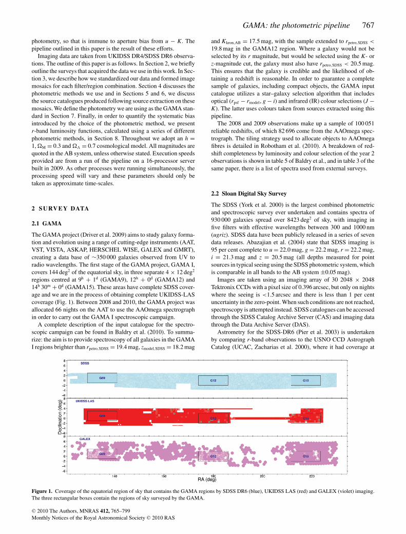
The GAMA project (Driver et al. 2009) aims to study galaxy forma-tion and evolution using a range of cutting-edge instruments (AAT,VST, VISTA, ASKAP, HERSCHEL WISE, GALEX and GMRT),creating a data base of ∼350 000 galaxies observed from UV toradio wavelengths. The first stage of the GAMA project, GAMA I,covers 144 deg2 of the equatorial sky, in three separate 4 × 12 deg2
regions centred at 9h + 1d (GAMA9), 12h + 0d (GAMA12) and14h 30m + 0d (GAMA15). These areas have complete SDSS cover-age and we are in the process of obtaining complete UKIDSS-LAScoverage (Fig. 1). Between 2008 and 2010, the GAMA project wasallocated 66 nights on the AAT to use the AAOmega spectrographin order to carry out the GAMA I spectroscopic campaign.
A complete description of the input catalogue for the spectro-scopic campaign can be found in Baldry et al. (2010). To summa-rize: the aim is to provide spectroscopy of all galaxies in the GAMAI regions brighter than rpetro,SDSS = 19.4 mag, zmodel,SDSS = 18.2 mag
and Kkron,AB = 17.5 mag, with the sample extended to rpetro,SDSS <
19.8 mag in the GAMA12 region. Where a galaxy would not beselected by its r magnitude, but would be selected using the K- orz-magnitude cut, the galaxy must also have rpetro,SDSS < 20.5 mag.This ensures that the galaxy is credible and the likelihood of ob-taining a redshift is reasonable. In order to guarantee a completesample of galaxies, including compact objects, the GAMA inputcatalogue utilizes a star–galaxy selection algorithm that includesoptical (rpsf − rmodel, g − i) and infrared (IR) colour selections (J −K). The latter uses colours taken from sources extracted using thispipeline.
The 2008 and 2009 observations make up a sample of 100 051reliable redshifts, of which 82 696 come from the AAOmega spec-trograph. The tiling strategy used to allocate objects to AAOmegafibres is detailed in Robotham et al. (2010). A breakdown of red-shift completeness by luminosity and colour selection of the year 2observations is shown in table 5 of Baldry et al., and in table 3 of thesame paper, there is a list of spectra used from external surveys.
2.2 Sloan Digital Sky Survey
The SDSS (York et al. 2000) is the largest combined photometricand spectroscopic survey ever undertaken and contains spectra of930 000 galaxies spread over 8423 deg2 of sky, with imaging infive filters with effective wavelengths between 300 and 1000 nm(ugriz). SDSS data have been publicly released in a series of sevendata releases. Abazajian et al. (2004) state that SDSS imaging is95 per cent complete to u = 22.0 mag, g = 22.2 mag, r = 22.2 mag,i = 21.3 mag and z = 20.5 mag (all depths measured for pointsources in typical seeing using the SDSS photometric system, whichis comparable in all bands to the AB system ±0.05 mag).
Images are taken using an imaging array of 30 2048 × 2048Tektronix CCDs with a pixel size of 0.396 arcsec, but only on nightswhere the seeing is <1.5 arcsec and there is less than 1 per centuncertainty in the zero-point. When such conditions are not reached,spectroscopy is attempted instead. SDSS catalogues can be accessedthrough the SDSS Catalog Archive Server (CAS) and imaging datathrough the Data Archive Server (DAS).
Astrometry for the SDSS-DR6 (Pier et al. 2003) is undertakenby comparing r-band observations to the USNO CCD AstrographCatalog (UCAC, Zacharias et al. 2000), where it had coverage at
Figure 1. Coverage of the equatorial region of sky that contains the GAMA regions by SDSS DR6 (blue), UKIDSS LAS (red) and GALEX (violet) imaging.The three rectangular boxes contain the regions of sky surveyed by the GAMA.
C© 2010 The Authors, MNRAS 412, 765–799Monthly Notices of the Royal Astronomical Society C© 2010 RAS

768 D. T. Hill et al.
the time of release, or Tycho-2 (Høg et al. 2000), when the UCACdid not have coverage. For sources brighter than r = 20 mag, theastrometric accuracy when compared to the UCAC is 45 mas andwhen compared to Tycho-2 is 75 mas. In both cases, there is a further30-mas systematic error and a relative error between filters (i.e. inugiz) of 25–35 mas.
The GAMA input catalogue is defined using data from the SDSSDR6 (Adelman-McCarthy et al. 2008). The GAMA regions fallwithin the SDSS DR6 area of coverage, in SDSS stripes 9–12.
2.3 UKIDSS
UKIDSS (Lawrence et al. 2007) is a 7-yr near-IR (NIR) surveyprogramme that will cover several thousand degrees of sky. Theprogramme utilizes the Wide Field Camera (WFCAM) on the 3.8-mUnited Kingdom Infra-Red Telescope (UKIRT). The UKIDSS pro-gramme consists of five separate surveys, each probing to a differentdepth and for a different scientific purpose. One of these surveys,the UKIDSS Large Area Survey (LAS), will cover 4000 deg2 andwill overlap with the SDSS stripes 9–16, 26–33 and part of stripe82. As the GAMA survey regions are within SDSS stripes 9–12, theLAS survey will provide high-density NIR photometric coverageover the entire GAMA area. The UKIDSS-LAS survey observesto a far greater depth (KLAS = 18.2 mag using the Vega magnitudesystem) than the previous Two-Micron All-Sky Survey (2MASS,K2MASS = 15.50 mag using the Vega magnitude system).
When complete, the LAS has target depths of K = 18.2 mag, H =18.6 mag, J = 19.9 mag (after two passes; this paper uses only thefirst J pass, which is complete to 19.5 mag) and Y = 20.3 mag (alldepths measured use the Vega system for a point source with 5σ
detection within a 2-arcsec aperture). Currently, observations havebeen conducted in the equatorial regions and will soon cover largeswathes of the Northern Sky. It is designed to have a seeing fullwidth at half-maximum (FWHM) of <1.2 arcsec, photometric rmsuncertainty of <±0.02 mag and astrometric rms of <±0.1 arcsec.Each position on sky will be viewed for 40 s per pass. All surveydata for this paper are taken from the fourth data release (DR4).
The WFCAM Science Archive (WSA, Hambly et al. 2008) is thestorage facility for post-pipeline, calibrated UKIDSS data. It pro-vides users with access to fits images and CASU-generated objectcatalogues for all five UKIDSS surveys. We do not use the CASU-generated catalogues for a few reasons. First, the CASU cataloguesfor early UKIDSS data releases suffer from a fault where deblendedobjects are significantly brighter than their parent object, in somecases by several magnitudes (Smith, Loveday & Cross 2009; Hillet al. 2010). Secondly, the CASU catalogues only contain circu-lar aperture fluxes. Thirdly, CASU decisions (e.g. deblending andaperture sizes) are not consistent between filters. For instance, theaperture radius and centre used to calculate KPETROMAG of a sourceis not necessarily the same as the aperture radius and centre used tocalculate YPETROMAG or HPETROMAG. We require accurate extended-aperture colours; the CASU catalogues do not provide this.
3 C O N S T RU C T I O N O F TH E M O S A I C SFROM SDSS AND UKIDSS IMAG ING
One of GAMA’s priorities is the accurate measurement of SEDsfrom as broad a wavelength range as possible. This is non-trivialwhen combining data from multiple surveys. While each surveymay be internally consistent with data collected contemporane-ously, conditions between surveys can vary. In particular, seeingand zero-point parameters may greatly differ between frames. When
matching between surveys, one may find an object in the centre ofthe frame in one survey split across two frames in another survey.There may also be variation in the angular scale of a pixel betweendifferent instruments and even when two instruments have the samepixel size; a shift of half of a pixel between two frames can causesignificant difficulties in calculating colours for small, low surfacebrightness objects. Furthermore, in order to use SEXTRACTOR in dualframe mode, the source-detection and the observation frame pix-els must be calibrated to the same world coordinate system. In theGAMA survey, we have attempted to circumvent these difficultiesby creating gigapixel-scale mosaics with a common zero-point andconsistent WCS calibration. The construction process is outlined inthis section.
To generate our image mosaics, we use the Terapix SWARP (Bertinet al. 2002) utility. This is a mosaic-generation tool and how weutilize it is described in Section 3.4. Before we can use this software,however, it is necessary for us to normalize the contributing SDSSand UKIDSS data to take into account differences in sky conditionsand exposure times between observations. For every file, we mustidentify its current zero-point (see the distribution in Fig. 2) and
Zeropoint (AB mag) u
Fre
quency
26.0 27.0 28.0 29.0
01000200030004000500060007000
Zeropoint (AB mag) g
Fre
quency
26.0 27.0 28.0 29.0
01000200030004000500060007000
Zeropoint (AB mag) r
Fre
quency
26.0 27.0 28.0 29.0
01000200030004000500060007000
Zeropoint (AB mag) i
Fre
quency
26.0 27.0 28.0 29.0
01000200030004000500060007000
Zeropoint (AB mag) z
Fre
quency
26.0 27.0 28.0 29.0
01000200030004000500060007000
Zeropoint (AB mag) Y
Fre
quency
26.0 27.0 28.0 29.0
0
500
1000
1500
2000
2500
3000
3500
Zeropoint (AB mag) J
Fre
quency
26.0 27.0 28.0 29.0
0
500
1000
1500
2000
2500
3000
3500
Zeropoint (AB mag) H
Fre
quency
26.0 27.0 28.0 29.0
0
500
1000
1500
2000
2500
3000
3500
Zeropoint (AB mag) K
Fre
quency
26.0 27.0 28.0 29.0
0
500
1000
1500
2000
2500
3000
3500
Figure 2. A histogram of the calculated total zero-points for the fields usedto create our master region mosaics.
C© 2010 The Authors, MNRAS 412, 765–799Monthly Notices of the Royal Astronomical Society C© 2010 RAS

GAMA: the photometric pipeline 769
transform it to a defined standard. This process is described inSections 3.1 and 3.2.
3.1 UKIDSS: acquisition of data and renormalizationto a common zero-point
UKIDSS imaging is stored within the WFCAM Science Archive(WSA). We downloaded 862 Y-, 883 J-, 931 H- and 928 K-bandcompressed UKIDSS-LAS fits files that contained images of skyfrom the GAMA regions. These files were decompressed usingthe IMCOPY utility. The files for each band are stored and treatedseparately.
A specially designed pipeline accesses each file, reads theMAGZPT (ZPmag), EXP_TIME (t), airmass [0.5 ∗ (AMSTART +AMEND) = secχmean] and EXTINCT (Ext) keywords from the fitsheader and creates a total AB magnitude zero-point for the file usingequation (1):
ZPtotal = ZPmag − 2.5 log
(1
t
)− Ext × (secχmean − 1) + ABVX,
(1)
where ABVX is the AB magnitude of Vega in the X band (Table 1).To correct each frame to a standard zero-point (30), the value of
each pixel is multiplied by a factor, calculated using equation (2).Whilst we show the distribution of frame zero-points in Fig. 2 in binsof 0.1 mag, we use the actual zero-point of each frame to calculatethe total AB magnitude zero-point. This has a far smaller variation(e.g. 0.02 mag in photometric conditions in the JHK filters; Warrenet al. 2007).
pixelmodifier = 10−0.4(ZPtotal−30). (2)
A new file is created to store the corrected pixel table and theMAGZPT fits header parameter is updated. The SKYLEVEL andSKYNOISE parameters are then scaled using the same multiplyingfactor. This process takes 3 s per file.
Table 1. Conversion to AB magni-tudes. The SDSS photometric systemis roughly equivalent to the AB mag-nitude system, with only small offsetsin the u and z passbands. UKIDSSphotometry is calculated on the Vegamagnitude system and our conver-sions are from Hewett et al. (2006).Whilst we convert UKIDSS data usinga high-precision parameter, it shouldbe noted that the conversion uncer-tainty is only known to ∼±0.02 mag(Cohen, Wheaton & Megeath 2003).
Band AB offset (mag)
u −0.04g 0r 0i 0z +0.02Y 0.634J 0.938H 1.379K 1.900
3.2 SDSS: acquisition of data and renormalizationto a common zero-point
The tsField and fpC files for the 12757 SDSS fields that coverthe GAMA regions were downloaded from the SDSS data archiveserver (das.sdss.org) for all five passbands. Again, the files for eachpassband are stored and treated separately.
We use a specially designed pipeline that brings in the ‘aa’ (zero-point), ‘kk’ (extinction coefficient) and ‘airmass’ keywords from afield’s tsField file, and the EXPTIME (t) keyword from the samefield’s fpC file. Combining these parameters using equation (3),we calculate the current total AB magnitude zero-point of the field(ZPtotal):
ZPtotal = −aa − 2.5 log(1/t) − kk × airmass + sAo, (3)
where ‘sAo’ is the offset between the SDSS magnitude system andthe actual AB magnitude system (−0.04 mag for u, 0.02 mag forz, otherwise 0). The SDSS photometric zero-point uncertainty isestimated to be no larger than 0.03 mag in any band (Ivezic et al.2004). We calculate the multiplier required to transform every pixelin the field (again using equation 2) to a standard zero-point (30).As every pixel must be modified by the same factor, we utilize theFCARITH program (part of the FTOOLS package) to multiply the entireimage by pixelmodifier. FCARITH can normalize an SDSS imageevery 1.25 s.
3.3 Correction of seeing bias
As observations were taken in different conditions, there is an intrin-sic seeing bias between different input images and between differentfilters (Fig. 3). This could cause inaccuracies in photometric colourmeasurements that use apertures defined in one filter to derive mag-nitudes in a second filter. To rectify this problem, it is necessary forus to degrade the better quality images to a lower seeing. However, ifwe degrade all images to our lowest quality seeing (3.12 arcsec), weshould lose the ability to resolve the smallest galaxies in our sample.Therefore, we elect to degrade our normalized images to 2-arcsecseeing. The fraction of images with seeing worse than 2 arcsec is4.4, 2.7, 2.5, 2.1, 1.7, 0, 0, 1.3 and 0.9 per cent in u, g, r, i, z, Y ,J, H and K, respectively. Images with worse seeing than 2 arcsecare included in our degraded seeing mosaics. We do not attempt tomodify their seeing. Although each survey uses a different methodof calculating the seeing within their data [the SDSS uses a doubleGaussian to model the point spread function (PSF), the UKIDSSuses the average FWHM of the stellar sources within the image],we assume that the seeing provided for every frame is correct.
To achieve a final PSF FWHM of 2 arcsec (σ final), we assume thatthe seeing within an image follows a perfect Gaussian distribution,σ initial. Theoretically, a Gaussian distribution can be generated fromthe convolution of two Gaussian distributions. The FGAUSS utility(also part of the FTOOLS package) can be used to convolve an inputimage with a circular Gaussian with a definable standard deviation(σ req), calculated using equation (4):
σreq =√
σ 2final − σ 2
initial. (4)
As each UKIDSS frame has a different seeing value, it is neces-sary to break each fits file into its four constituent images. This isnot necessary for SDSS images (which are stored in separate files).However, it is necessary to retrieve the SDSS image seeing fromthe image’s tsField file. The SDSS image seeing is stored in thepsf_width column of the tsField file. Where an image has a seeingbetter than our specified value, we use the FGAUSS utility to convolve
C© 2010 The Authors, MNRAS 412, 765–799Monthly Notices of the Royal Astronomical Society C© 2010 RAS

770 D. T. Hill et al.
Seeing (arcsec) u
Fre
quency
0.0 0.5 1.0 1.5 2.0 2.5 3.0
0500
100015002000250030003500
Seeing (arcsec) g
Fre
quency
0.0 0.5 1.0 1.5 2.0 2.5 3.0
0500
100015002000250030003500
Seeing (arcsec) r
Fre
quency
0.0 0.5 1.0 1.5 2.0 2.5 3.0
0500
100015002000250030003500
Seeing (arcsec) i
Fre
quency
0.0 0.5 1.0 1.5 2.0 2.5 3.0
0500
100015002000250030003500
Seeing (arcsec) z
Fre
quency
0.0 0.5 1.0 1.5 2.0 2.5 3.0
0500
100015002000250030003500
Seeing (arcsec) Y
Fre
quency
0.0 0.5 1.0 1.5 2.0 2.5 3.0
0
200
400
600
800
1000
1200
Seeing (arcsec) J
Fre
quency
0.0 0.5 1.0 1.5 2.0 2.5 3.0
0
200
400
600
800
1000
1200
Seeing (arcsec) H
Fre
quency
0.0 0.5 1.0 1.5 2.0 2.5 3.0
0
200
400
600
800
1000
1200
Seeing (arcsec) K
Fre
quency
0.0 0.5 1.0 1.5 2.0 2.5 3.0
0
200
400
600
800
1000
1200
Figure 3. A histogram of the calculated seeing of the fields used to createour master region mosaics.
our image down to our specified value. Where an image has a see-ing worse than our specified value, we copy it without modificationusing the IMCOPY utility. Both utilities produce a set of UKIDSSfiles containing two HDUs: the original instrument header HDUand a single image HDU with seeing greater than or equal to ourspecified seeing. The output SDSS files contain just a single imageHDU. This process takes approximately 2 s per frame.
3.4 Creation of master region images
The SWARP utility is a multithread capable co-addition andimage-warping tool that is part of the Terapix pipeline (Bertinet al. 2002). We use SWARP to generate complete images ofthe GAMA regions from the normalized LAS/SDSS fits files.It is vital that the pixel size and area of coverage are thesame for each filter, as SEXTRACTOR’s dual-image mode requiresperfectly matched frames. We define a pixel scale of 0.4 ×0.4 arcsec and generate 117 000 × 45 000 pixel files centred around09h00m00.s0, +01d00′00.′′0 (GAMA 9), 12h00m00.s0, +00d00′00.′′0(GAMA 12) and 14h 30m00.s0, +00d00′00.′′0 (GAMA 15). SWARP isset to resample input frames using the default LANCZOS3 algo-
Figure 4. The r-band weight map of the 45000 × 45000 pixel subset region(5 × 5 deg2; defined in Section 5). Joins and overlap between frames areapparent (light grey). The mosaic does not have imaging of the top right-hand corner or the bottom section (dark grey). These areas lie outside theregion of interest as the mosaics are slightly larger in Dec. than the GAMAregions themselves.
rithm, which the Terapix team found was the optimal option whenworking with images from the Megacam instrument (Bertin et al.2002).
SWARP produces mosaics that use the TAN WCS projection sys-tem. As UKIDSS images are stored in the ZPN projection system,SWARP internally converts the frames to the TAN projection sys-tem. There is also an astrometric distortion present in the UKIDSSimages that SWARP corrects using the pv2_3 and pv2_1 fits headerparameters.1
SWARP is set to subtract the background from the image, using abackground mesh of 256 × 256 pixels (102 × 102 arcsec) and a backfilter size of 3 × 3 to calculate the background map. The backgroundcalculation follows the same algorithm as SEXTRACTOR (Bertin &Arnouts 1996). To summarize: it is a bicubic-spline interpolationbetween the meshes, with a median filter applied to remove brightstars and artefacts.
Every mosaic contains pixels that are covered by multiple inputframes. SWARP is set to use the median pixel value when a number ofimages overlap. The effects of outlying pixel values, due to cosmicrays, bad pixels or CCD edges, should therefore be reduced. SWARP
generates a weight map (Fig. 4) that contains the flux variance in ev-ery pixel, calibrated using the background map described above. Asthe flux variance is affected by overlapping coverage, it is possibleto see the survey footprint in the weight map. The weight map canbe used within SEXTRACTOR to compensate for variations in noise.We do not use it when calculating our photometry for two reasons.First, there is overlap between SDSS fpC frames. This overlap isnot from observations, but from the method used to cut the longSDSS stripes into sections. SWARP would not account for this and
1 An analysis of the astrometric distortion can be found in theCASU document VDF-TRE-IOA-00009-0002, presently available athttp://www.ast.cam.ac.uk/vdfs/docs/reports/astrom/index.html
C© 2010 The Authors, MNRAS 412, 765–799Monthly Notices of the Royal Astronomical Society C© 2010 RAS

GAMA: the photometric pipeline 771
Figure 5. A comparison between the original normalized image and theK-band mosaic image of a galaxy on the bottom edge of an input UKIDSSframe. The bottom section of the galaxy is not part of this image and it hasbeen stitched together on the mosaic using SWARP.
the weighting of the overlap regions on the optical mosaics wouldbe calculated incorrectly. Secondly, using the weight maps wouldalter the effect of mosaic surface brightness limit variations uponour output catalogues. As we intend to model surface brightnesseffects later, we elect to use an unweighted photometric catalogue.
A small number of objects will be split between input frames.SWARP can reconstruct them, with only small defects due to CCDedges. One such example is shown in Fig. 5. We create both seeing-corrected and uncorrected mosaics for each passband and regioncombination. Each file is 20 Gb in size. In total, the mosaics requirejust over 1 Terabyte of storage space. Each mosaic takes approxi-mately 4 h to create.
4 PH OTO M E T RY
A major problem with constructing multiwavelength catalogues isthat the definition of what constitutes an object can change acrossthe wavelength range (see Appendix A, particularly Fig. A1). Thiscan be due to internal structure, such as dust lanes or star-formingregions, becoming brighter or fainter in different passbands, causingthe extraction software to deblend an object into a number of smallerparts in one filter but not in another. This can lead to large errorsin the resulting colours. We cannot be certain that the SDSS objectextraction process would produce the same results as the extractionprocess we use to create our UKIDSS object catalogues. Seeing,deblending and aperture sizes will differ, compromising colours. Tocreate a consistent multiwavelength sample, the photometry needsto be recalculated consistently across all nine filters. At the sametime, we can move from the circular apertures of the SDSS andUKIDSS to full elliptical apertures, as well as investigate a varietyof photometric methods. To generate our source catalogues, we usethe SEXTRACTOR software (Bertin & Arnouts 1996). This is an objectextraction utility and its use is described in Section 4.5.
In this paper, we implement four different methods to define ourobject positions and apertures. We produce three SEXTRACTOR cat-alogues (Bertin & Arnouts 1996) and one Sersic catalogue (basedupon GALFIT 3, Peng et al. 2007), in addition to the original SDSSdata set. The generation of the three new SEXTRACTOR catalogues isdetailed in Section 4.5. Each of the new SEXTRACTOR catalogues con-tains magnitudes calculated using two different elliptical, extendedsource apertures: the Kron and the Petrosian magnitude systems.They are briefly described in Sections 4.1–4.3. We also use a spe-cially designed pipeline (SIGMA GAMA, Kelvin et al. 2010, basedupon GALFIT 3) to calculate a total magnitude for each galaxy via
its best-fitting Sersic profile. This aperture system, and the processused to generate it, is described in Sections 4.4 and 4.6.
It is not obvious which photometric method will produce theoptimal solution. Whilst the Sersic photometric method solvesthe missing light problem, it requires higher quality data to calculatethe set of parameters that best model the galactic light profile. TheKron and Petrosian magnitude systems will work with lower qualitydata, but may underestimate the flux produced by a galaxy. In thissection, we describe the photometric systems that we have used.Later, in Sections 6 and 8, we will examine the different resultsproduced by the choice of the photometric system.
4.1 Self-defined Kron and Petrosian apertures
We construct an independent catalogue for each filter, containingelliptical Kron and Petrosian apertures. These independent cata-logues are then matched across all nine wavebands using STILTS (seeSection 4.7 and Taylor 2006). The apertures will therefore vary insize, potentially giving inconsistent colours, and as deblending de-cisions will also change, inconsistent matching between cataloguesmay occur. However, as the apertures are defined from the imagethey are used on, there can be no problem with magnitudes beingcalculated for objects that do not exist or with missing objects thatare not visible in the r band.
The self-defined catalogues are generated from the basic mosaics,where no attempt to define a common seeing for the mosaic has beenmade. This method should generate the optimal list of sources ineach band; however, as the precise definition of the source will varywith wavelength, the colours generated using this method will beinaccurate and subject to aperture bias. As the mosaic has variationsin seeing, the PSF will also vary across the image.
4.2 r-band-defined Kron and Petrosian apertures
We use SEXTRACTOR to define a sample of sources in the r-bandimage and then use the r-band position and aperture information tocalculate their luminosity within each filter (using the SEXTRACTOR
dual image mode). As the aperture definitions do not vary betweenwavebands, this method gives internally consistent colours and asthe list itself does not change, source matching between filters isunnecessary. However, where an object has changed in size (seeAppendix A), does not exist (e.g. an artefact in the r-band sample)or when the r-band aperture definition incorrectly includes multi-ple objects, the output colours may be compromised. Any objectthat is too faint to be visible within the r-band mosaic will alsonot be detected using this method. However, such objects will befainter than the GAMA sample’s selection criteria and would notbe included within our sample. The r-band-defined catalogues aregenerated from our seeing-degraded mosaics. They provide us withan optically defined source sample.
This method is analogous to the SDSS source catalogues, whichdefine their apertures using the r-passband data (unless the object isnot detected in r, in which case a different filter is chosen). However,the GAMA photometric pipeline has a broader wavelength range,as it now includes NIR measurements from the same aperture defi-nition. Furthermore, the SDSS Petrosian magnitudes have not beenseeing-standardized. While all data are taken at the same time, thediffraction limit is wavelength-dependent and different fractions oflight will be missed, despite the use of a fixed aperture. SDSS modelmagnitudes do account for the effects of the PSF.
C© 2010 The Authors, MNRAS 412, 765–799Monthly Notices of the Royal Astronomical Society C© 2010 RAS

772 D. T. Hill et al.
4.3 K-band-defined Kron and Petrosian apertures
This method works in the same way as the previous method, butuses the K-band image as the detection frame rather than the r-bandimage. We are limited in the total area, as the K-band coverage iscurrently incomplete. However, for samples that require completecolour coverage in all nine filters, this is not a problem. As withr-band-defined catalogues, the K-band-defined catalogues are gen-erated from the seeing-corrected mosaics. They provide us with aNIR-defined source sample. The K-band-defined Kron magnitudeswere used in the GAMA input catalogue (Baldry et al. 2010) tocalculate the star–galaxy separation J − K colour and the K-bandtarget selection.
4.4 Sersic magnitudes
We use the SIGMA modelling wrapper (see Section 4.6 and Kelvinet al. 2010 for more details), which in turn uses the galaxy-fittingsoftware GALFIT 3.0 (Peng et al. 2007) to fit a single-Sersic compo-nent to each object independently in nine filters (ugrizYJHK) andrecover their Sersic magnitudes, indices, effective radii, positionangles and ellipticities. Source positions are initially taken fromthe GAMA input catalogue, as defined in Baldry et al. (2010). AllSersic magnitudes are self-defined; as each band is modelled inde-pendently of the others, the aperture definition will vary and colourmay therefore be compromised.
Single-Sersic fitting is comparable to the SDSS model magni-tudes. SIGMA therefore should recover total fluxes for objects thathave a Sersic index in the range 0.3 < n < 20, where model magni-tudes force a fit to either an exponential (n = 1) or deVaucouleurs(n = 4) profile. The systematic magnitude errors that arise whenmodel magnitudes are fitted to galaxies that do not follow an ex-ponential or deVaucouleurs profile (Graham 2001; Brown et al.2003) do not occur in SIGMA. The SDSS team developed a com-posite magnitude system, CMODEL, which calculates a magnitudefrom the combination of the n = 1 and n = 4 systems, in orderto circumvent this issue (Abazajian et al. 2004). We compare ourSersic magnitudes to their results later. Sersic magnitudes do notsuffer from the missing-flux issue that affects Kron and Petrosianapertures. Petrosian magnitudes may underestimate a galaxy’s lu-minosity by 0.2 mag (Strauss et al. 2002), while under certain con-ditions, a Kron aperture may only recover half of a galaxy’s totalluminosity (Andreon 2002). The Sersic catalogues are generatedfrom the seeing-uncorrected mosaics, as the seeing parameters aremodelled within SIGMA using the PSFEX software utility (E. Bertin,private communication).
4.5 Object extraction of Kron and Petrosian apertures
The SEXTRACTOR utility (Bertin & Arnouts 1996) is a program thatgenerates catalogues of source positions and aperture fluxes from aninput image. It has the capacity to define the sources and aperturesin one frame and calculate the corresponding fluxes in a secondframe. This dual image mode is computationally more intensivethan the standard SEXTRACTOR single-image mode (in single-imagemode, SEXTRACTOR can extract a catalogue from a mosaic within afew hours; dual-image mode takes a few days per mosaic). Usingthe u, g, r, i, z, Y , J, H and K images created by the SWARP utility, wedefine our catalogue of sources independently (for the self-definedcatalogues), using the r-band mosaics (for the r-band-defined cat-alogue) or the K-band mosaics (for the K-band-defined catalogue),and calculate their flux in all nine bands. The normalization and
SWARP processes removed the image background and standardizedthe zero-point; we therefore use a constant MAG_ZEROPOINT =30 and BACK_VALUE = 0. SEXTRACTOR generates both ellipti-cal Petrosian- (2.0RPetro) and Kron-like apertures (2.5RKron, calledAUTO magnitudes). SEXTRACTOR Petrosian magnitudes are com-puted using 1
νRPetro= 0.2, the same parameter as the SDSS. As the
mosaics have been transformed on to the AB magnitude system, allmagnitudes generated by the GAMA photometric pipeline are ABmagnitudes.
The seeing convolution routine smooths out the backgroundand correlates the read noise of the images (this is apparent inFig. A1). As SEXTRACTOR detects objects of >xσ above the back-ground (where x is a definable parameter set to 1 in the defaultfile and for our seeing unconvolved catalogues), this assists in thedetection process, allowing SEXTRACTOR to find objects to a muchgreater depth, thus increasing the number of sources extracted usingthe standard setup. However, these new objects are generally muchfainter than the photometric limits of the GAMA spectroscopic cam-paign, many are false detections and the time required to generatethe source catalogues (particularly using SEXTRACTOR in dual-imagemode) is prohibitively large. Using a 10 000 × 10 000 pixel subsetof the GAMA9 r-band mosaic, we have attempted to calculate theDETECT_THRESH parameter that would output a catalogue of ap-proximately the same depth and size as the unconvolved cataloguewithin our spectroscopic limits (see Section 2.1). The distributionof objects with different DETECT_THRESH σ parameters, com-pared to the unconvolved catalogue, is shown in Fig. 6. We use aDETECT_MINAREA of 9 pixels. As the unconvolved catalogueis slightly deeper than the 2σ , but not as deep as the 1.7σ con-volved catalogue, we use a DETECT_THRESH parameter of 1.7σ
to generate our convolved catalogues. The 1.7 and 1σ catalogueshave consistent number counts to rAUTO = 21 mag, half a magni-tude beyond the rSDSS-band magnitude limit of the GAMA inputcatalogue.
rAUTO(mag)
N(m
) dm
50
100
500
10001000
5000
18 19 20 21 22 23 24 25
Detection threshold
1 sigma
1.2 sigma
1.5 sigma
1.7 sigma
Unconvolved 1 sigma
2 sigma
2.5 sigma
3 sigma
5 sigma
Figure 6. The effects of changing the SEXTRACTOR DETECT_THRESHparameter on a subset of an r-band mosaic. The dotted black line is thedeepest r-band sample limit of the GAMA survey (for those objects that areK or z selected).
C© 2010 The Authors, MNRAS 412, 765–799Monthly Notices of the Royal Astronomical Society C© 2010 RAS

GAMA: the photometric pipeline 773
Table 2. The names of the generated catalogues, the prescription used to create them and their abbreviatedfilename. The syntax in the Key column is summarized in Section 4.8.
Catalogue name Key Abbreviation
r-band-defined catalogue r[ugriz]SDSS + r[ugrizYJHK]GAMA:Petro,Kron catrdefSelf-defined catalogue r[ugriz]SDSS + {ugrizYJHK}GAMA:Petro,Kron catsd
K-band-defined catalogue r[ugriz]SDSS + K[ugrizYJHK]GAMA:Petro,Kron catKdefSersic catalogue r[ugriz]SDSS{ugrizYJHK}GAMA:Sersic catsers
GAMA master catalogue (r[ugriz]SDSS{r}GAMA:Sersic) + {ugrizYJHK}GAMA:Petro,Kron catmast
4.6 Object extraction for Sersic magnitudes
Sersic magnitudes are obtained as an output from the galaxy mod-elling program SIGMA (Structural Investigation of Galaxies viaModel Analysis) written in the R programming language (Kelvinet al. 2010). In brief, SIGMA takes the RA and Dec. of an objectthat has passed our star–galaxy separation criteria and calculates itspixel position within the appropriate mosaic. A square region, cen-tred on the object, is cut out from the mosaic containing a minimumof 20 guide stars with which to generate a PSF. SEXTRACTOR thenprovides a FITS-standard input catalogue to PSF EXTRACTOR (E.Bertin, private communication), which generates an empirical PSFfor each image. Ellipticities and position angles are obtained fromthe STSDAS ELLIPSE routine within IRAF, and provides an input toGALFIT. The larger cutout is again cut down to a region which con-tains 90 per cent of the target object’s flux plus a buffer of 10 pixelsand will only deviate from this size if a bright nearby object causesthe fitting region to be expanded in order to model any satellites thetarget may have.
GALFIT 3 is then used to fit a single-Sersic component to each targetand several runs may be attempted, if, for example, the previous runcrashed, the code reached its maximum number of iterations, thecentre has migrated to fit a separate object, the effective radius istoo high or low or the Sersic index is too large. SIGMA employs acomplex event handler in order to run the code as many times asnecessary to fix these problems; however, not all problems can befixed and so residual quality flags remain to reflect the quality ofthe final fit. The SIGMA package takes approximately 10 s per object.For full details of the SIGMA modelling program, see Kelvin et al.(2010).
4.7 Catalogue matching
The definition of the GAMA spectroscopic target selection (here-inafter referred to as the tiling catalogue) is detailed in Baldry et al.(2010) and is based on original SDSS DR6 data. We therefore needto relate our revised photometry back to this catalogue in order toconnect it to our AAOmega spectra. The tiling catalogue utilizesa mask around bright stars that should remove most objects withbad photometry and erroneously bright magnitudes, as well as im-plementing a revised star–galaxy separation quantified against ourspectroscopic results. It has been extensively tested, with sourcesthat are likely to be artefacts, bad deblends or sections of largergalaxies viewed a number of times by different people. By match-ing our catalogues to the tiling catalogue, we can access the resultsof this rigorous filtering process and generate a full, self-consistentset of colours for all of the objects that are within the GAMA sample(and are within regions that have been observed in all nine pass-bands). As the tiling catalogue is also used when redshift targeting,we will be able to calculate the completeness in all the passbandsof the GAMA survey. The GAMA tiling catalogue is a subset of
the GAMA master catalogue (hereinafter referred to as the mas-ter catalogue). The master catalogue is created using the SDSSDR6 catalogue stored on the CAS.2 Unlike the master catalogue,the tiling catalogue undertakes star–galaxy separation and appliessurface brightness and magnitude selection.
STILTS (Taylor 2006) is a catalogue combination tool, with a num-ber of different modes. We use it to join our region cataloguestogether to create r-band-defined, K-band-defined and self-definedaperture photometry catalogues that cover the entire GAMA area.We also use it to match these catalogues to the GAMA tiling cata-logue.
4.8 Source catalogues
The catalogues that have been generated are listed in Table 2. Thesyntax of the ‘Key’ column is as follows. X[u] means a u-bandmagnitude from an X-band-defined aperture, {u} means a self-defined u-band magnitude and ‘+’ denotes a STILTS tskymatch25-arcsec, unique nearest-object match between two catalogues (seeSection 4.7). Where two data sets are combined together without the‘+’ notation (i.e. the final two lines), this denotes a STILTS tmatch2,matcher = ‘exact’ match using SDSS objid as the primary key.Note that in a set of self-defined samples ({ugrizYJHK}), eachsample must be matched separately (as each contains a differentset of sources) and then combined. This is not the case in theaperture-defined samples (where each sample contains the sameset of sources). Subscripts denote the photometric method used foreach catalogue.
5 T E S T I N G TH E G A M A C ATA L O G U E S
In order to test the detection and deblending outcomes withinthe GAMA catalogues, a subsection of 25 deg2 has been chosenfrom near the centre of the GAMA 9 region (the pixels used are20 000–65 000 in the x-direction of the mosaic and 0–45 000 in they-direction). This region was chosen as it contains some of the is-sues facing the entire GAMA subset, such as area incompleteness.UKIDSS observations miss a large fraction of the subset area – ap-proximately 3.02 deg2 of the region has incomplete NIR coverage.The subset region was also chosen, because it partially contains anarea covered by the Herschel ATLAS science verification region(see Eales et al. 2010). Within this region, we ran SEXTRACTOR andcompared our results with the source lists produced by the SDSS
2 We use the query SELECT * FROM dr6.PhotoObj as p WHERE(p.modelmag_r − p.extinction_r < 20.5 or p.petromag_r − p.extinction_r <
19.8) and ((p.ra > 129.0 and p.ra < 141.0 and p.dec > −1.0 and p.dec <
3.0) or (p.ra > 174.0 and p.ra < 186.0 and p.dec > −2.0 and p.dec < 2.0)or (p.ra > 211.5 and p.ra < 223.5 and p.dec > −2.0 and p.dec < 2.0)) and(p.mode = 1) or (p.mode = 2 and p.ra < 139.939 and p.dec < −0.5 and(p.status & dbo.fphotostatus(’OK_SCANLINE’)) > 0)).
C© 2010 The Authors, MNRAS 412, 765–799Monthly Notices of the Royal Astronomical Society C© 2010 RAS

774 D. T. Hill et al.
and UKIDSS extraction software. Unless otherwise specified, allmagnitudes in this section were calculated using r-band-definedapertures.
5.1 Numerical breakdown
After generating source catalogues containing self-consistentcolours for all objects in the subset region (using the process de-scribed in Sections 4.5 and 4.7), we are left with an r-band aperture-defined subset region catalogue containing 1810 134 sources anda K-band aperture-defined subset region catalogue containing2298 224 sources (hereinafter referred to as the r-band and K-bandcatalogues, respectively). These catalogues contain many sourceswe are not interested in, such as sources with incomplete colourinformation, sources that are artefacts within the mosaics (satellitetrails, diffraction spikes, etc.), sources that are stars and sources thatare fainter than our survey limits.
The unfiltered r- and K-band catalogues were matched to themaster catalogue with a centroid tolerance of 5 arcsec, using theSTILTS tskymatch2 mode (see Section 4.7). Table 3 contains a break-down of the fraction of matched sources that have credible XAUTO
and XPETRO for all nine passbands (sources with incorrect AUTO orPETRO magnitudes have the value 99 as a placeholder; we impose acut at X = 50 to remove such objects). Generally, the low quality ofthe u-band SDSS images causes problems with calculating extendedsource magnitudes and this shows itself in the relatively high frac-tion of incomplete sources. This problem does not affect the otherSDSS filters to anywhere near the same extent. SDSS observationsdo not cover the complete subset area, but they have nearly completecoverage in both the r-band-defined (which is dependent on SDSSimaging) and the K-band-defined (reliant on UKIDSS coverage)catalogues. The UKIDSS observations cover a smaller section ofthe subset region, with the Y and J observations (taken separately tothe H and K) covering the least area of sky. This is apparent in ther-band catalogue, where at least 16 per cent of sources lack PETROor AUTO magnitudes in one or more passbands. By its definition,the K-band catalogue requires K-band observations to be present;as such there is a high level of completeness in the grizH and Kpassbands. However, the number of matched SDSS sources in theK-band catalogue itself is 4.2 per cent lower than in the r-bandcatalogue.
Table 3. Number of sources within the subset region with good SEXTRACTOR
XAUTO and XPETRO, where X is ugrizYJHK, from the r-or K-band-definedaperture catalogues matched to the GAMA master catalogue. The totalnumber of sources within the GAMA master catalogue for this region of skyis 138 233. per cent Cover is defined relative to r-band cover; where SDSScoverage does not exist, there are no GAMA master catalogue sources.
per cent per cent per centBand Cover Sources (r) (r) Sources (K) (K)
Total – 129 488 – 123 740 –u 100 111 403 86 105 801 86g 100 129 169 100 123 317 100r 100 129 481 100 123 610 100i 100 129 358 100 123 533 100z 100 128 287 99 122 479 99Y 88 108 167 84 109 672 89J 89 109 364 84 109 816 89H 96 121 212 94 121 846 98K 94 118 224 91 122 635 99
135 136 137 138 139
10
12
3
RA (degrees)
Declin
ation
( degre
es)
Figure 7. The RA and Dec. of SDSS objects that are not in either the r-or the K-band master-catalogue-matched catalogue. The darker areas note ahigh density of unmatched objects.
There are 138 233 master catalogue SDSS sources within the sub-set region. 119 330 SDSS objects have matches (within a 5-arcsectolerance) in both the r- and K-band master-catalogue-matched cat-alogues (this number is found by matching SDSS objid betweenthe catalogues). Those SDSS objects that do not have matches inboth master-catalogue-matched catalogues are shown in Fig. 7. Wedetail the reasons for the missing objects in Section 5.2.
5.2 SDSS sources missing in the master-catalogue-aperture-matched catalogues
There are 18 903 SDSS sources that are not found when the mas-ter catalogue is matched to either the r-band or the K-band-definedsubset region catalogues, 13.7 per cent of the total number of mastercatalogue sources within the subset region. Fig. 7 shows their distri-bution on sky. 8745 sources are not found within the r-band-definedcatalogue (6.3 per cent of the master catalogue sample) and 14 493are not found within the K-band-defined catalogue (10.5 per centof the sample), with 4335 of the sources unmatched to either the r-or the K-band-defined sample (3.1 per cent of the master cataloguesample). As the SDSS sample is defined by optical data, it is unsur-prising that a far larger number of sources are not found within theK-band-defined catalogue. Of the 18 903 unmatched master cata-logue sources, only 2367 have passed star–galaxy separation criteriaand are brighter than the GAMA spectroscopic survey magnitudelimits (r < 19.8 or zK selected).
Using r-band imaging, we have visually inspected all 8745 SDSSsources where our r-band-defined subset region catalogue cannotfind a match within 5 arcsec. Table 4 contains a summary of thereasons we do not find a r-band match. Using the SEXTRACTOR de-tection failure rate from the subset region as a guide to the detectionfailure rate for the entire GAMA region, SEXTRACTOR will miss ap-proximately 2.8 per cent of the objects recovered by the SDSS. Asecond problem was flagged through the inspection process; a fur-ther 1.7 per cent of the master catalogue sources within the subsetregion were not visible. Either these objects are low surface bright-
C© 2010 The Authors, MNRAS 412, 765–799Monthly Notices of the Royal Astronomical Society C© 2010 RAS

GAMA: the photometric pipeline 775
Table 4. A breakdown of the reasons for faulty detections in the 8745SDSS objects that are not matched to the r-band subset region catalogue.The images of the SDSS objects were generated from the standard r-bandGAMA mosaics and all 8745 objects were viewed by one observer (DTH).The criteria for selection are as follows. The first category is chosen in thosecases where an object has a nearby neighbour or may have been deblendedinto multiple sources by the SDSS algorithm. The second category is chosenwhere the position of the object is covered by a spike/trail. The third categoryis where a source is visible by eye. The fourth category is where a sourceis not visible above the noise. The fifth category is chosen when a source isobviously part of a larger structure. The sixth category is chosen when theSDSS data are of too low quality for visual classification to be undertaken.
Reason for non-detection Number Per cent of GAMA masterof objects catalogue subset region sample
Possible deblendingmismatch
601 0.4
Saturation spike/satelliteor asteroid trail
404 0.3
SEXTRACTOR detectionfailure
3831 2.8
Either a low surfacebrightness source or nosource
2391 1.7
Part of a large deblendedsource
1463 1.1
Low image qualitymaking detection difficult
55 0.04
ness extended objects, possibly detected in a different band, or theSDSS object extraction algorithm has made a mistake. A further1.8 per cent of sources within the GAMA master catalogue willbe missed by SEXTRACTOR due to differences in deblending deci-sions (either failing to split two sources or splitting one large objectinto a number of smaller parts), low SDSS image quality makingSEXTRACTOR fail to detect any objects or an artefact in the imagebeing accounted for by SEXTRACTOR (such as a saturation spike froma large star being detected as a separate object in the SDSS).
5.3 Sources in our r-band catalogue that are notin the GAMA master catalogue
To be certain that the SDSS extraction software is giving us a com-plete sample, we check whether our r-band subset region cataloguecontains sources that should be within the GAMA master catalogue,but are not. There are 61 351 sources within the r-band-defined sub-set region catalogue that have a complete set of credible AUTO andPETRO magnitudes, and are brighter than the GAMA spectroscopicsurvey limits. 619 of these sources do not have SDSS counterparts.We have visually inspected these sources; a breakdown is shown inTable 5. Similar issues cause missing detections using the SDSS orSEXTRACTOR algorithms. However, some of the unseen sources thatSEXTRACTOR detected may be due to the image convolution process(Section 3.3) gathering up the flux from a region with high back-ground noise and rearranging it so that it overcomes the detectionthreshold. Fig. 8 shows the distribution of rAUTO ≤ 20.5 mag sourcesdetected when SEXTRACTOR is run upon an original SDSS image file(covering ∼0.04 deg2) and the sources from the same file after it hasundergone the image convolution process. 233 sources are found inthe original SDSS frame and three additional sources are includedwithin the convolved frame sample. An examination of two sourcesthat are in the convolved frame data set and not in the original sam-ple shows the effect: these sources have rAUTO luminosities of 20.64
Table 5. A breakdown of the 619 r-band-defined subset region catalogueobjects brighter than the GAMA sample limits that are not matched to theGAMA master catalogue. The images of the subset region catalogue objectswere generated from the standard r-band GAMA mosaics and all 619 objectswere viewed by one observer (DTH).
Type of source Number of objects
Source 171No visible source 274
Section of bright star 163Possible deblend mismatch 10
Low image quality making detection difficult 1
Figure 8. A comparison between the objects detected when SEXTRACTOR
is run over an original SDSS image and when it is run over the convolved,mosaic imaging. Yellow circles are sources with r ≤ 20.5 mag detected fromthe GAMA mosaic and red crosses are sources that are detected from theoriginal SDSS data.
and 20.77 mag pre-convolution, but rAUTO luminosities of 20.40 and20.48 mag post-convolution.
Taking the SDSS non-detection rate within the subset region tobe the same as the non-detection rate over the entire GAMA region,we expect that the SDSS algorithm would have failed to detect0.1 per cent of sources brighter than the GAMA spectroscopicsurvey limits; approximately, 1000 sources would not have beenincluded within the master catalogue.
5.4 Sources in our K-band catalogue that are notin the UKIDSS DR5PLUS data base
We have also tested the UKIDSS DR5 catalogue. We have generateda catalogue from the WSA that selects all UKIDSS objects withinthe GAMA subset region3 and we have matched this catalogue to theK-band-defined subset region catalogue. From the 69 537 K-band-defined subset region catalogue sources, there are 4548 sources thathave not been matched to an UKIDSS object within a tolerance of5 arcsec. We have visually inspected K-band images of those ob-jects that are brighter than the GAMA spectroscopic survey K-bandlimit (KAUTO ≤ 17.6 mag). We find that 29 of the 117 unmatchedobjects are real sources that are missed by the UKIDSS extraction
3 We use the query ‘SELECT las.ra, las.dec, las.kPetroMag FROM lasSourceas las WHERE las.ra < 139.28 AND las.ra > 134.275 AND las.dec >−1AND las.dec <3’.
C© 2010 The Authors, MNRAS 412, 765–799Monthly Notices of the Royal Astronomical Society C© 2010 RAS

776 D. T. Hill et al.
software, a negligible fraction of the entire data set. A large (butunquantified) fraction of the other 88 sources are suffering from theconvolution flux-redistribution problem discussed in Section 5.3.The background fluctuations in K-band data are greater than in ther band, making this a much greater problem.
6 PRO P E RT I E S O F T H E C ATA L O G U E S
6.1 Constructing a clean sample
In order to investigate the photometric offsets between differentphotometric systems, we require a sample of galaxies with a com-plete set of credible photometry that are unaffected by deblendingdecisions. This has been created via the following prescription. Wematch the r-band-defined aperture catalogue to the GAMA mastercatalogue with a tolerance of 5 arcsec. We remove any GAMA ob-jects that have not been matched or have been matched to multipleobjects within that tolerance (when run in All match mode, STILTS
produces a GroupSize column, where a NULL value signifies nogroup). We then match to the nine self-defined object catalogues, ineach case removing all unmatched and multiply matched GAMAobjects. As our convolution routine will cause problems with thosegalaxies that contain saturated pixels, we also remove those galaxiesthat are flagged as saturated by the SDSS. This sample is then linkedto the Sersic pipeline catalogue (using the SDSS objid as the primarykey). We remove all those Sersic magnitudes where the pipelinehas flagged that the model is badly fitted or where the photome-try has been compromised and match the K-band aperture-definedcatalogue, again with unmatched and multiple matched sources re-moved. This gives us a final population of 18 065 galaxies thathave clean r-band-defined, K-band-defined, self-defined and Sersicmagnitudes, are not saturated and cannot be mismatched. Havingconstructed a clean, unambiguous sample of common objects, anyphotometric offset can only be due to differences between the pho-tometric systems used. As we remove objects that are badly fittedby the Sersic pipeline, it should be noted that the resulting samplewill, by its definition, only contain sources that have a light profilethat can be fitted using the Sersic function.
6.2 Photometric offset between systems
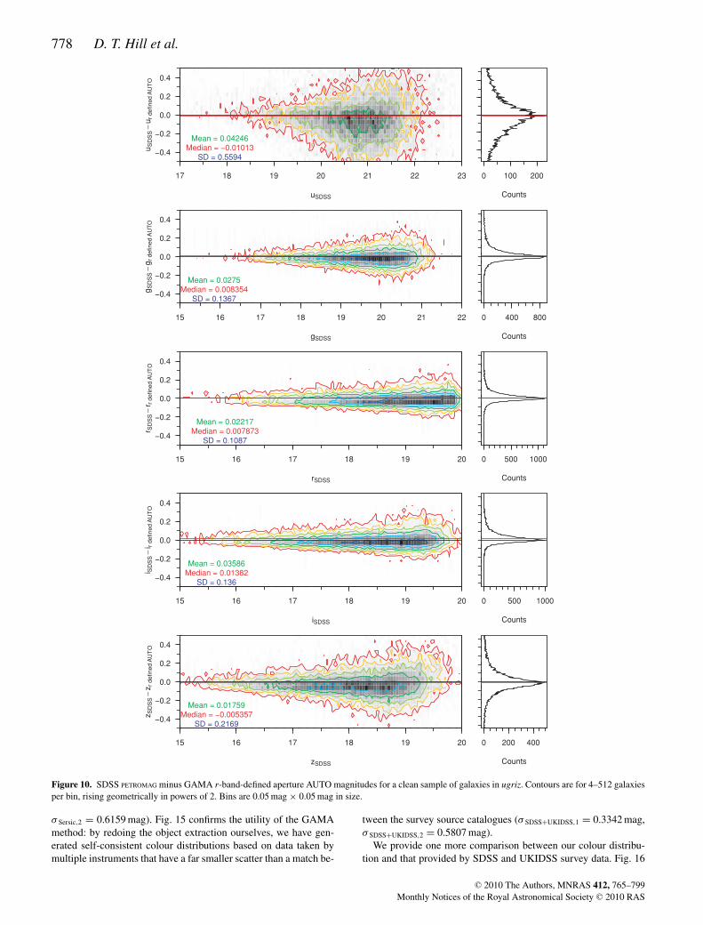
Figs 9–14 show the dispersion between different photometric sys-tems produced by this sample. In Fig. 9, we compare Kron andPetrosian magnitudes; in all other figures, we compare the photo-metric system to SDSS PETROMAG. In all photometry systems, thegri relationships are tightest, with the u and z relationships subjectto a greater scatter, breaking down almost entirely for Figs 12 and13. The correlation between the SDSS PETROMAG and the r-band-defined Petrosian magnitude (Fig. 11) looks much tighter than thatbetween the SDSS PETROMAG and the self-defined Petrosian magni-tude (Fig. 12). The standard deviations of the samples are similar,with marginally more scatter in the self-defined sample (0.129 magagainst 0.148 mag). The median offset between SDSS Petrosianand the r-band-defined Petrosian magnitudes, however, is 0.01 maggreater.
Fig. 13, illustrating the relationship between the Sersic magni-tude and the SDSS PETROMAG, produces median mSDSS − mSersic
values of 0.12, 0.06, 0.06, 0.07 and 0.09 mag in ugriz. These val-ues can be compared to those presented in fig. 13 of Blanton et al.(2003) (−0.14, 0.00, 0.06, 0.09 and 0.14 mag at z = 0.1, using the0.1ugriz filters), given the variance in the relationship (the standarddeviations in our samples are 0.77, 0.28, 0.21, 0.22 and 0.40 mag,
respectively). A significant fraction (∼28 per cent) of the sample hasrSDSS − rSersic > 0.5 mag and therefore lies beyond the boundaries ofthis image. These offsets are significant and will be discussed furtherin Section 7. We can say that the r-band-defined aperture photom-etry is the closest match to SDSS PETROMAG photometry. Fig. 14shows the relationship between the GAMA Sersic magnitude andthe optimal model magnitude provided by the SDSS (CMODEL). Themodel magnitudes match closely, with negligible systematic offsetbetween the photometric systems in gri.
6.3 Colour distributions
In order to identify the optimal photometric system, we assumethat intrinsic colour distribution of a population of galaxies can beapproximated by a double-Gaussian distribution (the superpositionof a pair of Gaussian distributions with different mean and standarddeviation parameters). This distribution can model the bimodalityof the galaxy population. The presence of noise will broaden thedistribution; hence, the narrowest colour distribution reveals theoptimal photometric system for calculating the colours of galax-ies and therefore deriving accurate SEDs. Fig. 15 shows the (u −r) and (r − K) colour distributions for each photometric system,for objects within our subset region. In order to calculate the dis-persion in the colour distribution, we generate colour-distributionhistograms (with bins of 0.1 mag) and find the double-Gaussiandistribution parameters that best fit each photometric system. Thebest-fitting standard deviation parameters for each sample are shownat the bottom of each plot and are denoted by σ X,1 and σ X,2 (whereX is the photometric system fitted). The sample with the small-est set of σ parameters should provide the optimal photometricsystem.
The SDSS, GAMA r-band-defined aperture and GAMA K-band-defined distributions (the first, third and fourth diagrams on the toptwo rows) show a very similar pattern, a tight distribution of ob-jects with a small number of red outliers. As expected, when weuse apertures that are defined separately in each filter (the seconddiagram on the top two rows), the colour distribution of the popula-tion is more scattered (σ Petro,1 = 0.7576 mag, σ Petro,2 = 0.7919 mag,σ AUTO,1 = 0.5886 mag, σ AUTO,2 = 0.7086 mag) and does not showthe bimodality visible in the matched aperture photometry (at thebright end of the distribution, there are two distinct subpopulations– one subpopulation above u − r = 2 mag and the other below).For the same reason, and probably because of the low quality ofthe observations, the (u − r) plot using the Sersic magnitudes (thefinal diagram on the top row) has the broadest colour distribution(σ Sersic,1 = 0.6242 mag, σ Sersic,2 = 1.098 mag), although it is wellbehaved in (r − K).
To generate a series of (r − K) colours using the UKIDSS survey(leftmost plot on the bottom two rows), we have taken all galaxieswithin the UKIDSS catalogue4 and match them (with a maximumtolerance of 5 arcsec) to a copy of the tiling catalogue that hadpreviously been matched with the K-band aperture-defined cata-logue. The distribution of (r − K) colours taken from the SDSSand UKIDSS survey catalogues is the first diagram on the bot-tom two rows of the image. As the apertures used to define theUKIDSS and SDSS sources are not consistent, we find that thetightest (r − K) distribution comes from the GAMA K-band-defined
4 We run a query at the WSA on UKIDSSDR5PLUS looking for all objects withinour subset region with lasSource.pGalaxy >0.9 and lasSource.kPetroMag<20 – equivalent to KAB < 21.9 mag.
C© 2010 The Authors, MNRAS 412, 765–799Monthly Notices of the Royal Astronomical Society C© 2010 RAS

GAMA: the photometric pipeline 777
ur defined petro
ur
de
fin
ed
AU
TO
−u
r d
efin
ed
PE
TR
O
17 18 19 20 21 22 23
0.0
0.2
0.4
4SD = 0.4267
Counts
0 200 400
gr defined petro
gr
de
fin
ed
AU
TO
−g
r d
efin
ed
PE
TR
O
15 16 17 18 19 20 21 22
0.0
0.2
0.4
SD = 0.09574
Counts
0 500 1000
rr defined petro
r r d
efin
ed
AU
TO
−r r
de
fin
ed
PE
TR
O
15 16 17 18 19 20
0.0
0.2
0.4
1SD = 0.04886
Counts
0 700 1400
ir defined petro
i r d
efin
ed
AU
TO
−i r
de
fin
ed
PE
TR
O
15 16 17 18 19 20
0.0
0.2
0.4
SD = 0.0644
Counts
0 700
zr defined petro
zr
de
fin
ed
AU
TO
−z
r d
efin
ed
PE
TR
O
15 16 17 18 19 20
0.0
0.2
0.4
SD = 0.2068
Counts
0 300 600
Figure 9. GAMA r-band-defined aperture Petrosian minus AUTO magnitudes for a clean sample of galaxies in ugriz. Contours are for 4–512 galaxies perbin, rising geometrically in powers of 2. Bins are 0.05 mag × 0.05 mag in size.
aperture sample (fourth from the left-hand side on the bottom row,with σ AUTO,1 = 0.3137 mag, σ AUTO,2 = 0.4921 mag). The GAMAsample that relies on matching objects between self-defined objectcatalogues (the second diagram on the bottom two rows) has the
broadest distribution (σ Petro,1 = 0.3359 mag, σ Petro,2 = 0.6015 mag).The distribution of sources in the Sersic (r − K) colour plot is muchtighter than in (u − r), though still not as tight as the distributionin the fixed aperture photometric systems (σ Sersic,1 = 0.364 mag,
C© 2010 The Authors, MNRAS 412, 765–799Monthly Notices of the Royal Astronomical Society C© 2010 RAS
778 D. T. Hill et al.
uSDSS
uS
DS
S−
ur
de
fin
ed
AU
TO
17 18 19 20 21 22 23
0.0
0.2
0.4
Mean = 0.04246
SD = 0.5594
Counts
0 100 200
gSDSS
gS
DS
S−
gr
de
fin
ed
AU
TO
15 16 17 18 19 20 21 22
0.0
0.2
0.4
Median = 0.008354Mean = 0.0275
SD = 0.1367
Counts
0 400 800
rSDSS
r SD
SS
−r r
de
fin
ed
AU
TO
15 16 17 18 19 20
0.0
0.2
0.4
Median = 0.007873Mean = 0.02217
SD = 0.1087
Counts
0 500 1000
iSDSS
i SD
SS
−i r
de
fin
ed
AU
TO
15 16 17 18 19 20
0.0
0.2
0.4
Median = 0.01382Mean = 0.03586
SD = 0.136
Counts
0 500 1000
zSDSS
zS
DS
S−
zr
de
fin
ed
AU
TO
15 16 17 18 19 20
0.0
0.2
0.4
Mean = 0.01759
SD = 0.2169
Counts
0 200 400
Figure 10. SDSS PETROMAG minus GAMA r-band-defined aperture AUTO magnitudes for a clean sample of galaxies in ugriz. Contours are for 4–512 galaxiesper bin, rising geometrically in powers of 2. Bins are 0.05 mag × 0.05 mag in size.
σ Sersic,2 = 0.6159 mag). Fig. 15 confirms the utility of the GAMAmethod: by redoing the object extraction ourselves, we have gen-erated self-consistent colour distributions based on data taken bymultiple instruments that have a far smaller scatter than a match be-
tween the survey source catalogues (σ SDSS+UKIDSS,1 = 0.3342 mag,σ SDSS+UKIDSS,2 = 0.5807 mag).
We provide one more comparison between our colour distribu-tion and that provided by SDSS and UKIDSS survey data. Fig. 16
C© 2010 The Authors, MNRAS 412, 765–799Monthly Notices of the Royal Astronomical Society C© 2010 RAS

GAMA: the photometric pipeline 779
uSDSS
uS
DS
S−
ur
de
fin
ed
PE
TR
O
17 18 19 20 21 22 23
0.0
0.2
0.4
Median = 0.02481Mean = 0.04529
SD = 0.7049
Counts
0 100
gSDSS
gS
DS
S−
gr
de
fin
ed
PE
TR
O
15 16 17 18 19 20 21 22
0.0
0.2
0.4
Median = 0.03758Mean = 0.05751
SD = 0.1815
Counts
0 300 600
rSDSS
r SD
SS
−r r
de
fin
ed
PE
TR
O
15 16 17 18 19 20
0.0
0.2
0.4
Median = 0.02932Mean = 0.03904
SD = 0.128
Counts
0 400 800
iSDSS
i SD
SS
−i r
de
fin
ed
PE
TR
O
15 16 17 18 19 20
0.0
0.2
0.4
Median = 0.046Mean = 0.06997
SD = 0.1581
Counts
0 300 600
zSDSS
zS
DS
S−
zr
de
fin
ed
PE
TR
O
15 16 17 18 19 20
0.0
0.2
0.4
Median = 0.02074Mean = 0.02549
SD = 0.3097
Counts
0 200 400
Figure 11. SDSS PETROMAG minus GAMA r-band-defined aperture Petrosian magnitudes for a clean sample of galaxies in ugriz. Contours are for 4–512galaxies per bin, rising geometrically in powers of 2. Bins are 0.05 mag × 0.05 mag in size.
displays the X − H distribution produced by the GAMA galax-ies with complete ugrizYJHK photometry and good-quality red-shifts within 0.033 < z < 0.6. The effective wavelengths of thefilter set for each galaxy are shifted using the redshift of the
galaxy. The colour distribution provided by the GAMA photom-etry produces fewer outliers than the SDSS/UKIDSS survey datasample and is well constrained by the Bruzual & Charlot (2003)models.
C© 2010 The Authors, MNRAS 412, 765–799Monthly Notices of the Royal Astronomical Society C© 2010 RAS

780 D. T. Hill et al.
uSDSS
uS
DS
S−
use
lf d
efin
ed
PE
TR
O
17 18 19 20 21 22 23
0.0
0.2
0.4
SD = 0.9021
Counts
0 20 40 60
gSDSS
gS
DS
S−
gse
lf d
efin
ed
PE
TR
O
15 16 17 18 19 20 21 22
0.0
0.2
0.4
Median = 0.01687Mean = 0.02562
SD = 0.2343
Counts
0 120 240
rSDSS
r SD
SS
−r s
elf d
efin
ed
PE
TR
O
15 16 17 18 19 20
0.0
0.2
0.4
Median = 0.01962Mean = 0.02459
SD = 0.1455
Counts
0 200 400
iSDSS
i SD
SS
−i s
elf d
efin
ed
PE
TR
O
15 16 17 18 19 20
0.0
0.2
0.4
Median = 0.01313Mean = 0.02266
SD = 0.1541
Counts
0 200 400
zSDSS
zS
DS
S−
zse
lf d
efin
ed
PE
TR
O
15 16 17 18 19 20
0.0
0.2
0.4
SD = 0.395
Counts
0 80 160
Figure 12. SDSS PETROMAG minus GAMA self-defined aperture Petrosian magnitudes for a clean sample of galaxies in ugriz. Contours are for 4–512 galaxiesper bin, rising geometrically in powers of 2. Bins are 0.05 mag × 0.05 mag in size.
7 FI NA L G A M A P H OTO M E T RY
Sections 5 and 6 show that the optimal deblending outcome isproduced by the original SDSS data, but the best colours come
from our r-band-defined aperture photometry (Section 6.3). We seethat our r-band-defined aperture photometry agrees with the SDSSPETROMAG photometry. However, we have also demonstrated thatSDSS PETROMAG misses flux when compared to our Sersic total
C© 2010 The Authors, MNRAS 412, 765–799Monthly Notices of the Royal Astronomical Society C© 2010 RAS

GAMA: the photometric pipeline 781
uSDSS
uS
DS
S−
uS
ers
ic
17 18 19 20 21 22 23
0.0
0.2
0.4
Median = 0.1219Mean = 0.1914
SD = 0.7736
Counts
0 50
gSDSS
gS
DS
S−
gS
ers
ic
15 16 17 18 19 20 21 22
0.0
0.2
0.4
Median = 0.05956Mean = 0.1392
SD = 0.2835
Counts
0 150 300
rSDSS
r SD
SS
−r S
ers
ic
15 16 17 18 19 20
0.0
0.2
0.4
Median = 0.06339Mean = 0.1207
SD = 0.2142
Counts
0 200
iSDSS
i SD
SS
−i S
ers
ic
15 16 17 18 19 20
0.0
0.2
0.4
Median = 0.07318Mean = 0.1314
SD = 0.2239
Counts
0 200
zSDSS
zS
DS
S−
zS
ers
ic
15 16 17 18 19 20
0.0
0.2
0.4
Median = 0.08752Mean = 0.1724
SD = 0.3963
Counts
0 80 160
Figure 13. SDSS PETROMAG minus GAMA Sersic magnitudes for a clean sample of galaxies in ugriz. Contours are for 4–512 galaxies per bin, risinggeometrically in powers of 2. Bins are 0.05 mag × 0.05 mag in size.
magnitude. Here we combine these data sets to arrive at our finalphotometry. We combine the SDSS deblending outcome with ourr-band-defined aperture colours and the Sersic total magnitude toproduce our best photometric solution.
7.1 Sersic magnitudes
To check the reliability of the Sersic photometry pipeline, wemust examine its distribution against a photometric system we
C© 2010 The Authors, MNRAS 412, 765–799Monthly Notices of the Royal Astronomical Society C© 2010 RAS

782 D. T. Hill et al.
uSDSS,cmodel
uS
DS
S,c
mo
de
l−u
Se
rsic
17 18 19 20 21 22 23
0.0
0.2
0.4
SD = 0.7703
Counts
0 50
gSDSS,cmodel
gS
DS
S,c
mo
de
l−g
Se
rsic
15 16 17 18 19 20 21 22
0.0
0.2
0.4
MMean = 0.07536
SD = 0.2804
Counts
0 150 300
rSDSS,cmodel
r SD
SS
,cm
od
el−
r Se
rsic
15 16 17 18 19 20
0.0
0.2
0.4
Median = 0.008772Mean = 0.06861
SD = 0.2148
Counts
0 200 400
iSDSS,cmodel
i SD
SS
,cm
od
el−
i Se
rsic
15 16 17 18 19 20
0.0
0.2
0.4
Median = 0.007943Mean = 0.07177
SD = 0.2244
Counts
0 200 400
zSDSS,cmodel
zS
DS
S,c
mo
de
l−z
Se
rsic
15 16 17 18 19 20
0.0
0.2
0.4
Mean = 0.07234
SD = 0.3774
Counts
0 80 160
Figure 14. SDSS CMODEL minus GAMA Sersic magnitudes for a clean sample of galaxies in ugriz. Contours are for 4–512 galaxies per bin, rising geometricallyin powers of 2. Bins are 0.05 mag × 0.05 mag in size.
consider reliable. We examine the distribution of the Sersic photom-etry against our r-band-defined AUTO photometry. Fig. 17 showsthe distribution of Sersic–GAMA r-band-defined AUTO magni-tude against r-band-defined AUTO magnitude for all objects in the
GAMA sample that have passed our star–galaxy separation criteriaand have credible AUTO magnitudes. Whilst there is generally atight distribution, the scatter in the u band, in particular, is a causefor concern.
C© 2010 The Authors, MNRAS 412, 765–799Monthly Notices of the Royal Astronomical Society C© 2010 RAS

GAMA: the photometric pipeline 783
Figure 15. A comparison between the u − r and r − K colours produced using SDSS MODELMAG, GAMA self-defined Petrosian magnitudes, GAMA r/K-band-defined Petrosian magnitudes, Sersic and GAMA total magnitudes for objects in the subset region. Contours shown are for 2–512 galaxies per bin, risinggeometrically in powers of 2. Bins are 0.1 mag in width in each axis. The σ parameter comes from the best-fitting bivariate-Gaussian distribution, when it isfitted to the colour-distribution histogram in each plot.
C© 2010 The Authors, MNRAS 412, 765–799Monthly Notices of the Royal Astronomical Society C© 2010 RAS

784 D. T. Hill et al.
Figure 16. A comparison between the X − H colours produced using SDSS magnitudes and GAMA total magnitudes. Data come from all GAMA galaxieswith good-quality redshifts (0.033 < z < 0.6) and complete ugrizYJHK photometry. Effective wavelengths are calculated from the redshift of the galaxy and thefilter effective wavelength, and the data set is binned into a 50 × 50 bin matrix. Two Bruzual-Charlot 03 SSP instantaneous-burst models are also plotted. Bothmodels use the Chabrier (2003) initial mass function, with mass cut-offs at 0.1 and 100 M�. Stellar evolution is undertaken using the Padova 1994 prescription.The dark grey line is a model evolved to 11 Gyr, with Z = 0.05 and Y = 0.352. The purple line is a model evolved to 0.25 Gyr, using Z = 0.02 (Z�) andY = 0.28.
Graham et al. (2005) analytically calculate how the ratio of Sersicflux to Petrosian flux changes with the Sersic index of the object.The fraction of light missed by a Petrosian aperture is dependentupon the light profile of the source. Fig. 19 shows the distribu-tion of Sersic–GAMA r-band-defined Petrosian magnitude againstthe Sersic index, redshift, absolute and apparent magnitude for allr-band objects in the GAMA sample that have passed our star–galaxy separation criteria, and have credible r, u and K r-band-defined PETRO magnitudes. Graham et al. report a 0.20-mag offsetfor an n = 4 profile and a 0.50-mag offset for an n = 8 profile.The median rSersic − rPetrosian offset for objects with 3.9 < n < 4.1in this sample is −0.115 mag, with rms scatter of 0.212 mag, and−0.408 mag, for objects with 7.9 < n < 8.1, with rms scatter of0.292 mag. Both results agree with the reported values. We haveplotted the magnitude offset with Sersic index function from fig. 2(Panel a) of Graham et al. (2005) in the uppermost plot of Fig. 19.
The function is an extremely good match to our photometry. Fig. 18shows the distribution of Sersic–SDSS CMODEL magnitude againstthe Sersic index, redshift, absolute and apparent magnitude for allr-band objects in the GAMA sample that have passed our star–galaxy separation criteria, and have credible r, u and K r-band-defined PETRO magnitudes. The distributions are very similar tothose produced by the Sersic–Petrosian colours in Fig. 19. An ex-ception is the distribution with the Sersic index, where the Sersic–CMODEL offset is distributed closer to 0 mag, until n = 4, at whichpoint the Sersic magnitude detects more flux. As the CMODEL mag-nitude is defined as a combination of n = 1 and n = 4 profiles, it isunsurprising that it cannot model high-n profile sources as well asthe GAMA Sersic magnitude, which allows the n-parameter greaterfreedom.
The r-band Sersic magnitude shows no anomalous behaviour.Sersic profiling is reliable when undertaken using the higher
C© 2010 The Authors, MNRAS 412, 765–799Monthly Notices of the Royal Astronomical Society C© 2010 RAS

GAMA: the photometric pipeline 785
Figure 17. Sersic minus GAMA r-band-defined AUTO magnitude against r-band-defined AUTO magnitude, in all nine bands, for all objects in the GAMAsample that pass our star–galaxy separation criteria and have credible ugrizYJHK r-band-defined AUTO magnitudes. Contours increase geometrically in powersof 2, from 4 to 512. Bins are 0.1 mag (x-axis) × 0.05 mag (y-axis) in size.
quality SDSS imaging (particularly gri), but not when using thenoisier u-band data. It is clear that the u-band Sersic magnitude isnot robust enough to support detailed scientific investigations. Inorder to access a Sersic-style total magnitude in the u band, weare therefore forced to create one from existing, reliable data. Wedevise such an approach in Section 7.2.
7.2 ‘Fixed aperture’ Sersic magnitudes
As mentioned in Section 4.4, the Sersic magnitude is taken from adifferent aperture in each band. We therefore cannot use Sersic mag-nitudes to generate accurate colours (the scatter in the Sersic coloursis compared to that in the AUTO colours in Fig. 20). We also donot consider the u, b and Sersic magnitudes to be credible (see Sec-tion 7.1). However, we also believe that the r-band Sersic luminosityfunction may be more desirable than the light-distribution-definedaperture r-band luminosity functions. The calculation of the totalluminosity density using a non-Sersic aperture system may under-
estimate the parameter. We require a system that accounts for theadditional light found by the Sersic magnitude, but also provides acredible set of colours.
We derive a further magnitude Xtotal, using the equation Xtotal =(XAUTO − rAUTO) + rSersic, where ‘AUTO’ is the r-band-definedAUTO magnitude. In effect, this creates a measure that combinesthe total r-band flux with optimal colours, using SDSS deblendingto give us the most accurate catalogue of sources (by matching to theGAMA master catalogue); the best of all possibilities. We acceptthat this assumes that the colour from the r-band-defined AUTOaperture would be the same as the colour from a r-band-definedSersic aperture; however, this is the closest estimation to a fixedSersic aperture we can make at this time.
7.3 Uncertainties within the photometry
The gain value in SDSS data is constant within each stripe, butvaries between stripes. The SDSS mosaic creation process that is
C© 2010 The Authors, MNRAS 412, 765–799Monthly Notices of the Royal Astronomical Society C© 2010 RAS

786 D. T. Hill et al.
Sersic Index
r Sers
ic−
r cm
odel
0.2 0.5 1 2 5
0.0
0.5
rcmodel
r Sers
ic−
r cm
odel
16 17 18 19 20
0.0
0.5
ZSPEC
r Sers
ic−
r cm
odel
0.0 0.1 0.2 0.3 0.4
0.0
0.5
Mr,Sersic
r Sers
ic−
r cm
odel
0.0
0.5
Figure 18. Sersic r − SDSS CMODEL r magnitude against the Sersic index, SDSS r CMODEL magnitude, z, Mr,Sersic for all objects in the GAMA sample thathave passed our star–galaxy separation criteria and have credible urK r-band-defined Petrosian magnitudes. Contours increase geometrically in powers of 2,from 4 to 512.
C© 2010 The Authors, MNRAS 412, 765–799Monthly Notices of the Royal Astronomical Society C© 2010 RAS

GAMA: the photometric pipeline 787
Figure 19. Sersic r − GAMA r-band-defined Petrosian r against the Sersic index, r-band-defined r-band Petrosian magnitude, z, Mr,Sersic for all objects in theGAMA sample that have passed our star–galaxy separation criteria and have credible urK r-defined Petrosian magnitudes. Contours increase geometrically inpowers of 2, from 4 to 512. The brown function plotted in the Sersic r − GAMA r-band-defined Petrosian r against the Sersic index plot is taken from fig. 2(upper panel) of Graham et al. (2005).
C© 2010 The Authors, MNRAS 412, 765–799Monthly Notices of the Royal Astronomical Society C© 2010 RAS

788 D. T. Hill et al.
1012345 uAUTO − rAUTO
u−
r
1
0
1
2 gAUTO − rAUTO
g−
r
1
0
1
2 rAUTO − iAUTO
r−
i
1
0
1
2
3
rAUTO − zAUTO
r−
z
1
0
1
2
3
rAUTO − YAUTO
r−
Y
1
0
1
2
3rAUTO − JAUTO
r−
J
1
0
1
2
3rAUTO − HAUTO
r−
H
1
0
1
2
3
16 17 18 19 20
rAUTO − KAUTO
rAUTO
r−
K
uSersic − rSersic
gSersic − rSersic
rSersic − iSersic
rSersic − zSersic
rSersic − YSersic
rSersic − JSersic
rSersic − HSersic
16 17 18 19 20
rSersic − KSersic
rSersic
uSDSS − rSDSS
gSDSS − rSDSS
rSDSS − iSDSS
16 17 18 19 20
rSDSS − zSDSS
rSDSS
Figure 20. X − r distributions from GAMA r-band-defined AUTO magnitudes, GAMA Sersic magnitudes and SDSS PETROMAGs (left-hand to right-handpanel), against r, for all X = u, g, i, z, Y , J, H and K. Sources used are those within the subset region with credible AUTO and Sersic magnitudes and withoutthe SDSS-saturated object bit set. Contours increase geometrically in powers of 2, from 2 to 512 galaxies bin−1. Bins are 0.1 mag × 0.1 mag in size.
C© 2010 The Authors, MNRAS 412, 765–799Monthly Notices of the Royal Astronomical Society C© 2010 RAS

GAMA: the photometric pipeline 789
0.01 0.02 0.03 0.04 0.05 0.06 0.07
1
2
3
4
5
6
7
8
9
10
11
12
13
14
15
σSDSS and all AUTO+PETRO r band magnitudes (mag)
r defined S
Extr
acto
r M
AG
ER
R_A
UT
O_r
(x10
−3m
ag)
Figure 21. The distribution of standard deviation in the r-band apparentmagnitude against SEXTRACTOR’s calculated magnitude error (using the firstquartile gain from the gain distribution of the mosaic’s input images) forour clean sample of galaxies, using SDSS, r-band-defined, K-band-definedand self-defined AUTO and PETRO magnitudes to calculate the standarddeviation. Contours rise linearly by 16 galaxies bin−1, ranging from 8 to 120galaxies bin−1. Bins are 0.004 mag (x-axis) × 0.001 mag (y-axis) in size.
detailed in Sections 3.2 and 3.4 combines images from a number ofdifferent stripes to generate the master mosaic. As the mosaics aretransformed from different zero-points, the relationship betweenelectrons and pixel counts will be different for each image. Thismosaic must suffer from variations in gain. The SEXTRACTOR utilitycan be set up to deal with this anomaly, by using the weightmapsgenerated by SWARP. However, this may introduce a level of surfacebrightness bias into the resulting catalogue that would be difficultto quantify. We calculate the SEXTRACTOR magnitude error via thefirst quartile value, taken from the distribution of gain parametersused to create the mosaic. The gain used in the SDSS calculation isthe average for the strip. The SEXTRACTOR error is calculated usingequation (5), where A is the area of the aperture, σ is the standarddeviation in noise and F is the total flux within the aperture. Byusing the first quartile gain value, we may be slightly overestimat-ing the F
gain component of the magnitude uncertainty calculation.However, given the amount of background noise in the mosaic, thiscomponent will constitute only a small fraction towards the error inthe fainter galaxies, and in the brighter galaxies, the uncertainty inmagnitude due to the aperture definition will be much greater thanthe SEXTRACTOR magnitude error itself. The SEXTRACTOR magnitudeerror is calculated separately for each aperture type and is availablewithin the GAMA photometric catalogues:
m =1.0857
√Aσ 2 + F
gain
F. (5)
We have attempted to quantify the uncertainty due to the aperturedefinition, in order to calculate its extent relative to the SEXTRACTOR
magnitude error. We use the cleaned sample defined in Section 6.1.The dispersion in calculated magnitude between our different photo-metric methods for this sample is shown in Figs 9–13. Fig. 21 showsthe relative scales of the uncertainty due to a galaxy’s aperture defini-tion (calculated from the standard deviation in AUTO/PETRO lumi-
rSDSS Petro
σ SD
SS
, a
ll A
uto
an
d a
ll P
etr
o m
ag
nitu
de
s
17.0 17.5 18.0 18.5 19.0 19.5
0
0.01
0.02
0.03
0.04
0.05
0.06
0.07
0.08
0.09
0.1
0.11
rSDSS Petro
σ SD
SS
, r
de
fin
ed
Au
to a
nd
Pe
tro
ma
gn
itu
de
s
17.0 17.5 18.0 18.5 19.0 19.5
0
0.01
0.02
0.03
0.04
0.05
0.06
0.07
0.08
0.09
0.1
0.11
rSDSS Petro
σ SD
SS
, se
lf d
efin
ed
Au
to a
nd
Pe
tro
ma
gn
itu
de
s
17.0 17.5 18.0 18.5 19.0 19.5
0
0.01
0.02
0.03
0.04
0.05
0.06
0.07
0.08
0.09
0.1
0.11
rSDSS Petro
σ SD
SS
, K
de
fin
ed
Au
to a
nd
Pe
tro
ma
gn
itu
de
s
17.0 17.5 18.0 18.5 19.0 19.5
0
0.01
0.02
0.03
0.04
0.05
0.06
0.07
0.08
0.09
0.1
0.11
Figure 22. The distribution of standard deviation in the r-band apparentmagnitude against apparent magnitude for our clean sample of galaxies,using four different sets of magnitudes to calculate the standard deviation ineach case. Contours rise linearly by 20 galaxies bin−1, ranging from 10 to170 galaxies bin−1. Bins are 0.1 mag (x-axis) × 0.01 mag (y-axis) in size.
nosities from the SDSS survey and our r/K/self-defined catalogues)and the error generated by SEXTRACTOR in the r band. The aper-ture definition uncertainty is generally much greater than that dueto background variation and signal-to-noise ratio that SEXTRACTOR
derives. Fig. 22 shows how this standard deviation in a galaxy’sr-band magnitude changes with apparent magnitude. Whilst thisuncertainty is larger than the SEXTRACTOR magnitude error, it isfundamentally a more consistent judgement of the uncertainty in agiven galaxy’s brightness as it does not assume that any particularextended-source aperture definition is correct. Whilst the dispersionof the relationship increases with apparent magnitude (along withthe number of galaxies), the modal standard deviation is approxi-mately constant. Taking this to be a good estimate of the averageuncertainty in the apparent magnitude of a galaxy within our sam-ple, we have confidence in our published apparent magnitudes towithin ±0.03 mag in gri, ±0.06 mag in z and ±0.20 mag in u. Wecalculate the same statistics in the NIR passbands (though withoutSDSS PETROMAG). We have confidence in our published apparentmagnitudes within ±0.05 mag in YJHK, approximately two and ahalf times the size of the photometric rms error the UKIDSS wasdesigned to have (±0.02 mag, Lawrence et al. 2007).
7.4 Number counts
In order to construct a unbiased data set, it is necessary for us tocalculate the apparent magnitude where the GAMA sample ceasesto be complete. Table 6 illustrates the size and depth of the GAMAapparent magnitude limited samples. This section describes thedefinition of these samples.
7.4.1 Definition of a GAMA galaxy sample used in this section
The GAMA sample used in this section is defined as those SDSSobjects that are within the area that has complete ugrizYJHK colour
C© 2010 The Authors, MNRAS 412, 765–799Monthly Notices of the Royal Astronomical Society C© 2010 RAS

790 D. T. Hill et al.
1
5
10
50
100
500
1000
mr defined AUTO
N d
m (
mag
−1d
eg
−2)
13 14 15 16 17 18 19 20 21
u
g
r
i
z
Y
J
H
K
Figure 23. Number counts of GAMA galaxies (sources that have passed our star–galaxy separation criteria) with good ugrizYJHK colours, split into 0.1-magbins and divided by the total area they cover. Error bars shown are for Poissonian number counts.
coverage and have passed the star–galaxy separation criteria. Of the908 022 objects in the GAMA master catalogue, only 124 622 fulfilthis criteria. The area of sky that has complete GAMA ugrizYJHKcoverage is 129.1232 ± 0.0008 deg2, 89.7 per cent of the entireGAMA region. All magnitudes in this section are r-band-definedAUTO magnitudes, unless otherwise defined.
7.4.2 Determination of apparent magnitude limits
Fig. 23 shows how the sky density of GAMA galaxies in the ninepassbands varies with apparent magnitude. The distributions peakin the 0.1-mag bins centred at u = 21.25, g = 20.55, r = 19.75,i = 19.25, z = 18.75, Y = 18.65, J = 18.45, H = 18.05 and K =17.75 mag. Tables 7–9 contain the number counts of GAMA galax-ies in ugrizYJHK, this time using 0.25-mag bins. Poissonian uncer-tainties are also included. Both sets of data have been converted todeg−2 mag−1 units.
The r-band number count drop-off, despite hitting the PETRO-MAG_R = 19.8 mag GAMA main sample magnitude limit, is notabsolute, because the SDSS limit was extended to PETROMAG_R =20.5 mag in the GAMA 12 region, so that useful filler objects couldbe selected, and because radio/K/z-band-selected objects in G9 andG15 will also be included within the catalogue. Objects that arefainter than rmodel = 20.5 mag (722 sources; 0.5 per cent of the
Table 6. The number of sources within the star–galaxy separation andapparent magnitude-limited GAMA samples that have a complete set ofgood ugrizYJHK r-band-defined magnitudes, the number of those sourcesthat have redshifts from first- and second-year data and the percentageredshift completeness. Apparent magnitudes are r-band-defined magnitudes,using the AB magnitude system.
Band Sources Redshifts Per cent redshifts
Star–galaxy separationcriteria only
124 622 82 926 66.5
u ≤ 21.0 46 006 39 767 86.4g ≤ 20.3 67 913 58 956 86.8r ≤ 19.8 106 032 79 672 75.1i ≤ 19.0 74 885 66 981 89.4z ≤ 18.5 59 470 55 202 92.8Y ≤ 18.4 57 739 53 339 92.4J ≤ 18.2 60 213 54 264 90.1H ≤ 17.8 55 734 51 033 91.6K ≤ 17.5 46 424 43 252 93.2
sample) will be due to differences in object extraction between theSDSS and SEXTRACTOR, as mentioned in previous sections.
The turnovers in Fig. 23 will occur where the r = 19.8 mag limitis reached for galaxies with the median passband − r colour. We are
C© 2010 The Authors, MNRAS 412, 765–799Monthly Notices of the Royal Astronomical Society C© 2010 RAS

GAMA: the photometric pipeline 791
Table 7. Number counts for the ugr filters, using r-band-defined AUTO photometry, with Poissonianuncertainties.
u(mag)
Nu(m)±σNu(m)
[deg−2 (mag)−1]g(mag)
Ng(m) ± σNg (m)
[deg−2 (mag)−1]r(mag)
Nr (m) ± σNr (m)
[deg−2 (mag)−1]
12.125 0.031 ± 0.015 10.125 0 ± 0 10.125 0.031 ± 0.01512.375 0 ± 0 10.375 0 ± 0 10.375 0 ± 012.625 0 ± 0 10.625 0 ± 0 10.625 0 ± 012.875 0 ± 0 10.875 0.031 ± 0.015 10.875 0.031 ± 0.01513.125 0 ± 0 11.125 0 ± 0 11.125 0 ± 013.375 0.031 ± 0.015 11.375 0 ± 0 11.375 0.124 ± 0.03113.625 0.093 ± 0.027 11.625 0.031 ± 0.015 11.625 0.062 ± 0.02213.875 0.062 ± 0.022 11.875 0 ± 0 11.875 0 ± 014.125 0.093 ± 0.027 12.125 0.062 ± 0.022 12.125 0.031 ± 0.01514.375 0.062 ± 0.022 12.375 0.124 ± 0.031 12.375 0.031 ± 0.01514.625 0.062 ± 0.022 12.625 0.031 ± 0.015 12.625 0.062 ± 0.02214.875 0.062 ± 0.022 12.875 0.031 ± 0.015 12.875 0.155 ± 0.03515.125 0.124 ± 0.031 13.125 0.031 ± 0.015 13.125 0.217 ± 0.04115.375 0.248 ± 0.044 13.375 0.062 ± 0.022 13.375 0.186 ± 0.03815.625 0.279 ± 0.046 13.625 0.062 ± 0.022 13.625 0.558 ± 0.06615.875 0.527 ± 0.064 13.875 0.248 ± 0.044 13.875 0.589 ± 0.06816.125 0.929 ± 0.085 14.125 0.248 ± 0.044 14.125 0.712 ± 0.07416.375 1.735 ± 0.116 14.375 0.712 ± 0.074 14.375 1.425 ± 0.10516.625 1.828 ± 0.119 14.625 0.62 ± 0.069 14.625 1.611 ± 0.11216.875 2.478 ± 0.139 14.875 0.836 ± 0.08 14.875 3.16 ± 0.15617.125 3.098 ± 0.155 15.125 1.27 ± 0.099 15.125 3.253 ± 0.15917.375 4.616 ± 0.189 15.375 2.478 ± 0.139 15.375 4.771 ± 0.19217.625 6.01 ± 0.216 15.625 2.447 ± 0.138 15.625 6.536 ± 0.22517.875 8.457 ± 0.256 15.875 4.089 ± 0.178 15.875 8.333 ± 0.25418.125 11.772 ± 0.302 16.125 4.213 ± 0.181 16.125 13.352 ± 0.32218.375 17.1 ± 0.364 16.375 6.32 ± 0.221 16.375 17.286 ± 0.36618.625 22.273 ± 0.415 16.625 9.139 ± 0.266 16.625 24.783 ± 0.43818.875 31.815 ± 0.496 16.875 13.166 ± 0.319 16.875 34.2 ± 0.51519.125 44.763 ± 0.589 17.125 16.728 ± 0.36 17.125 46.808 ± 0.60219.375 58.58 ± 0.674 17.375 24.225 ± 0.433 17.375 64.28 ± 0.70619.625 84.973 ± 0.811 17.625 31.722 ± 0.496 17.625 85.933 ± 0.81619.875 117.159 ± 0.953 17.875 42.719 ± 0.575 17.875 118.491 ± 0.95820.125 159.754 ± 1.112 18.125 58.673 ± 0.674 18.125 151.452 ± 1.08320.375 211.736 ± 1.281 18.375 74.502 ± 0.76 18.375 200.955 ± 1.24820.625 282.831 ± 1.48 18.625 101.299 ± 0.886 18.625 271.524 ± 1.4520.875 351.602 ± 1.65 18.875 132.122 ± 1.012 18.875 347.885 ± 1.64121.125 396.304 ± 1.752 19.125 170.256 ± 1.148 19.125 454.357 ± 1.87621.375 386.731 ± 1.731 19.375 222.175 ± 1.312 19.375 575.729 ± 2.112
19.625 282.428 ± 1.479 19.625 695.832 ± 2.32119.875 356.559 ± 1.662 19.875 540.445 ± 2.04620.125 446.148 ± 1.85920.375 505.471 ± 1.97920.625 492.894 ± 1.954
within the domain where the number of galaxies within a magnitudebin increases linearly with increasing apparent magnitude, but a de-viation from this relationship is visible in the figure, approximately3-mag bins before the turnover occurs in all bands except r. Thiseffect is due to colour incompleteness becoming a factor. Unfortu-nately, despite our radio/K/z selection, there will be a populationof objects that are bright in other passbands, but too faint in r tobe included within our sample. Assuming the passband − r colourdistribution is approximately Gaussian, this population will featurepredominantly in the apparent magnitude bins near the turnover,causing the characteristic flattening we see. Accounting for this ef-fect, we define the apparent magnitude sample limits of our sampleto be a few bins brighter than this turnover, where the linear rela-tionship still holds. Our apparent magnitude limits are set to u =21.0, g = 20.3, r = 19.8, i = 19.0, z = 18.5, Y = 18.4, J = 18.2,H = 17.8 and K = 17.6 mag.
7.4.3 GAMA apparent-magnitude-limited catalogues
Table 6 contains the sizes of the apparent-magnitude-limited sam-ples and their current redshift completeness. Our magnitude-limitedoptical samples contain approximately 40 000 less galaxies than theequivalent samples in Blanton et al. (2003), which covers the SDSSDR2 region, but extend 2 mag deeper. When we compare our num-ber counts to 6dFGS (Jones et al. 2009), our samples are also smallerin area coverage, but similar in size and much deeper in magnitudecompleteness. Hill et al. (2010), our previous attempt at defininga sample across the optical and NIR (combining MGC, SDSS andUKIDSS data to form a B-band-selected ugrizYJHK catalogue), wasjust one-tenth of the size and was 0.2–1.8 mag shallower. Currently,a large fraction of our samples have not been spectroscopically sam-pled. After the completion of the 2008–09 allocations of AAOmegaspectroscopy, our apparent magnitude samples have ≥75 per cent
C© 2010 The Authors, MNRAS 412, 765–799Monthly Notices of the Royal Astronomical Society C© 2010 RAS

792 D. T. Hill et al.
Table 8. Number counts for the izY filters, using r-band-defined AUTO photometry, with Poissonianuncertainties.
i(mag)
Ni (m) ± σNi (m)
[deg−2 (mag)−1]z(mag)
Nz(m) ± σNz(m)
[deg−2 (mag)−1]Y(mag)
NY (m) ± σNY (m)
[deg−2 (mag)−1]
9.375 0 ± 0 9.375 0 ± 0 9.375 0.031 ± 0.0159.625 0 ± 0 9.625 0.031 ± 0.015 9.625 0 ± 09.875 0.031 ± 0.015 9.875 0 ± 0 9.875 0.031 ± 0.01510.125 0 ± 0 10.125 0.031 ± 0.015 10.125 0 ± 010.375 0.031 ± 0.015 10.375 0 ± 0 10.375 0 ± 010.625 0 ± 0 10.625 0.124 ± 0.031 10.625 0.124 ± 0.03110.875 0.124 ± 0.031 10.875 0.031 ± 0.015 10.875 0.031 ± 0.01511.125 0.031 ± 0.015 11.125 0.031 ± 0.015 11.125 0.031 ± 0.01511.375 0.031 ± 0.015 11.375 0 ± 0 11.375 0 ± 011.625 0 ± 0 11.625 0.031 ± 0.015 11.625 0.062 ± 0.02211.875 0.031 ± 0.015 11.875 0.031 ± 0.015 11.875 0.062 ± 0.02212.125 0.031 ± 0.015 12.125 0.093 ± 0.027 12.125 0.093 ± 0.02712.375 0.186 ± 0.038 12.375 0.217 ± 0.041 12.375 0.186 ± 0.03812.625 0.186 ± 0.038 12.625 0.248 ± 0.044 12.625 0.217 ± 0.04112.875 0.124 ± 0.031 12.875 0.31 ± 0.049 12.875 0.403 ± 0.05613.125 0.372 ± 0.054 13.125 0.558 ± 0.066 13.125 0.651 ± 0.07113.375 0.682 ± 0.073 13.375 0.62 ± 0.069 13.375 0.743 ± 0.07613.625 0.62 ± 0.069 13.625 1.022 ± 0.089 13.625 1.022 ± 0.08913.875 0.96 ± 0.086 13.875 1.611 ± 0.112 13.875 1.673 ± 0.11414.125 1.704 ± 0.115 14.125 1.983 ± 0.124 14.125 2.478 ± 0.13914.375 2.168 ± 0.13 14.375 3.501 ± 0.165 14.375 3.779 ± 0.17114.625 3.748 ± 0.17 14.625 4.554 ± 0.188 14.625 4.585 ± 0.18814.875 3.965 ± 0.175 14.875 5.545 ± 0.207 14.875 6.289 ± 0.22115.125 5.917 ± 0.214 15.125 8.116 ± 0.251 15.125 9.015 ± 0.26415.375 8.302 ± 0.254 15.375 11.555 ± 0.299 15.375 13.506 ± 0.32315.625 10.749 ± 0.289 15.625 16.697 ± 0.36 15.625 17.689 ± 0.3715.875 16.635 ± 0.359 15.875 21.994 ± 0.413 15.875 25.774 ± 0.44716.125 22.211 ± 0.415 16.125 32.031 ± 0.498 16.125 34.727 ± 0.51916.375 31.598 ± 0.495 16.375 43.4 ± 0.58 16.375 49.937 ± 0.62216.625 40.984 ± 0.563 16.625 61.43 ± 0.69 16.625 69.484 ± 0.73416.875 60.872 ± 0.687 16.875 83.703 ± 0.805 16.875 93.802 ± 0.85217.125 82.464 ± 0.799 17.125 113.318 ± 0.937 17.125 124.873 ± 0.98317.375 111.367 ± 0.929 17.375 151.266 ± 1.082 17.375 161.83 ± 1.1217.625 142.995 ± 1.052 17.625 198.849 ± 1.241 17.625 221.277 ± 1.30917.875 193.397 ± 1.224 17.875 264.213 ± 1.43 17.875 292.124 ± 1.50418.125 253.432 ± 1.401 18.125 356.156 ± 1.661 18.125 375.424 ± 1.70518.375 336.423 ± 1.614 18.375 458.973 ± 1.885 18.375 480.285 ± 1.92918.625 438.093 ± 1.842 18.625 561.2 ± 2.085 18.625 549.831 ± 2.06418.875 549.336 ± 2.063 18.875 582.39 ± 2.12419.125 649.457 ± 2.24319.375 564.205 ± 2.09
completeness. It is anticipated that this statistic will rise to ≥95 percent after the completion of the 2010 allocation.
7.5 Incorporating GALEX data
We have also combined the GAMA sample with UV data. TheGAMA master catalogue has been matched to GALEX photometry(Wyder et al. 2005). As GALEX observations are of low resolu-tion (typical imaging FWHM ∼10 arcsec), the matching is complexcompared to the simple UKIDSS/SDSS matching described in thispaper as a number of separate SDSS objects may be matched toone larger GALEX object. The precise method of generating theGALEX matches is described in Robotham et al. (in preparation).In summary, all SDSS objects within the 90 per cent Petrosian ra-dius of a GALEX source are considered to be contributing flux tothat source. The flux of the GALEX object is then apportioned to
the SDSS objects, with the alloted fraction calculated via the dis-tance between the SDSS and GALEX objects. If no other nearbysource is within 2.5 mag (in g) of the closest match, then all flux isassigned to the closest match. GALEX has two distinct filters NUVand FUV . The generated magnitudes are stored within columnslabelled MAG_AUTO_FUV and MAG_AUTO_NUV .
7.6 SED fits using GAMA data
The SEDs of 10 galaxies selected at random from the GAMA sampleare shown in Fig. 24. We show the GAMA–GALEX UV luminosi-ties, GAMA total luminosities, Petrosian luminosities taken fromthe UKIDSS and SDSS surveys, and two Bruzual–Charlot (Bruzual& Charlot 2003) galaxy models with different ages and metallic-ities. The models are normalized via least-squares best fitting tothe nine GAMA data points. For image clarity, we do not show the
C© 2010 The Authors, MNRAS 412, 765–799Monthly Notices of the Royal Astronomical Society C© 2010 RAS

GAMA: the photometric pipeline 793
Table 9. Number counts for the JHK filters, using r-band-defined AUTO photometry, with Poissonianuncertainties.
J(mag)
NJ (m) ± σNJ (m)
[deg−2 (mag)−1]H(mag)
NH (m) ± σNH (m)
[deg−2 (mag)−1]K(mag)
NK (m) ± σNK (m)
[deg−2 (mag)−1]
9.125 0 ± 0 9.125 0.031 ± 0.015 9.125 0 ± 09.375 0 ± 0 9.375 0 ± 0 9.375 0.031 ± 0.0159.625 0.031 ± 0.015 9.625 0.031 ± 0.015 9.625 0 ± 09.875 0.031 ± 0.015 9.875 0 ± 0 9.875 0.031 ± 0.01510.125 0 ± 0 10.125 0.093 ± 0.027 10.125 0.031 ± 0.01510.375 0.062 ± 0.022 10.375 0.062 ± 0.022 10.375 0.062 ± 0.02210.625 0.062 ± 0.022 10.625 0.031 ± 0.015 10.625 0.031 ± 0.01510.875 0.062 ± 0.022 10.875 0 ± 0 10.875 0.062 ± 0.02211.125 0 ± 0 11.125 0 ± 0 11.125 0 ± 011.375 0 ± 0 11.375 0.031 ± 0.015 11.375 0 ± 011.625 0.031 ± 0.015 11.625 0.124 ± 0.031 11.625 0.062 ± 0.02211.875 0.124 ± 0.031 11.875 0.155 ± 0.035 11.875 0.062 ± 0.02212.125 0.155 ± 0.035 12.125 0.248 ± 0.044 12.125 0.186 ± 0.03812.375 0.217 ± 0.041 12.375 0.372 ± 0.054 12.375 0.217 ± 0.04112.625 0.31 ± 0.049 12.625 0.527 ± 0.064 12.625 0.31 ± 0.04912.875 0.527 ± 0.064 12.875 0.774 ± 0.077 12.875 0.682 ± 0.07313.125 0.712 ± 0.074 13.125 0.867 ± 0.082 13.125 0.867 ± 0.08213.375 0.898 ± 0.083 13.375 1.518 ± 0.108 13.375 1.022 ± 0.08913.625 1.549 ± 0.11 13.625 2.23 ± 0.131 13.625 1.735 ± 0.11613.875 2.076 ± 0.127 13.875 3.098 ± 0.155 13.875 2.478 ± 0.13914.125 3.191 ± 0.157 14.125 4.492 ± 0.187 14.125 3.903 ± 0.17414.375 4.43 ± 0.185 14.375 6.041 ± 0.216 14.375 5.545 ± 0.20714.625 5.7 ± 0.21 14.625 7.806 ± 0.246 14.625 7.621 ± 0.24314.875 8.147 ± 0.251 14.875 12.763 ± 0.314 14.875 10.192 ± 0.28115.125 12.639 ± 0.313 15.125 17.72 ± 0.37 15.125 17.689 ± 0.3715.375 17.224 ± 0.365 15.375 24.194 ± 0.433 15.375 23.915 ± 0.4315.625 24.163 ± 0.433 15.625 35.036 ± 0.521 15.625 35.966 ± 0.52815.875 33.425 ± 0.509 15.875 49.379 ± 0.618 15.875 49.999 ± 0.62216.125 46.715 ± 0.601 16.125 70.413 ± 0.738 16.125 77.879 ± 0.77716.375 66.448 ± 0.717 16.375 94.298 ± 0.855 16.375 109.198 ± 0.9216.625 92.222 ± 0.845 16.625 133.237 ± 1.016 16.625 158.422 ± 1.10816.875 121.434 ± 0.97 16.875 176.792 ± 1.17 16.875 218.272 ± 1.317.125 162.976 ± 1.123 17.125 245.781 ± 1.38 17.125 305.631 ± 1.53817.375 220.348 ± 1.306 17.375 319.602 ± 1.573 17.375 406.031 ± 1.77317.625 288.159 ± 1.494 17.625 420.931 ± 1.806 17.625 488.99 ± 1.94617.875 384.191 ± 1.725 17.875 504.448 ± 1.977 17.875 491.716 ± 1.95118.125 464.796 ± 1.897 18.125 515.229 ± 1.99818.375 521.394 ± 2.009
uncertainties on SDSS and UKIDSS data points. GAMA UV un-certainties are taken from SEXTRACTOR magnitude errors. GAMAoptical and NIR uncertainties are calculated using the standard de-viation in the luminosity when different photometric methods areused (following the method described in Section 7.3). In some cases,the photometry provided by survey catalogues and the GAMA pho-tometry are near identical and match the galaxy models well (see216774 and 137440 on Fig. 24). In other cases, where there isa discrepancy between our derived luminosities and the survey-catalogue parameters, the GAMA photometry is a better fit to themodels (e.g. 202588 and 518102 on Fig. 24). We therefore judgeour r-band-defined AUTO colours to be a significant improvement.
7.7 Released GAMA photometry
The GAMA photometry described in this paper provides theGamaPhotom catalogue. This catalogue is filtered and combinedwith the other GAMA catalogues to produce the first GAMA datarelease, defined in Driver et al. (2010).
8 TH E I M PAC T O F T H E PH OTO M E T R I CM E T H O D O N T H E O B S E RV E D LU M I N O S I T YDI STRI BU TI ON
8.1 Comparison between r-band luminosity functions
In order to illustrate the effect that photometric methods have onstatistical measurements of the galaxy population, we derive ther-band luminosity function using nine different photometric meth-ods. We use all our photometric systems and the original SDSSphotometry, and derive luminosity functions from the same popula-tion of galaxies. This should provide a consistent analysis for eachmethod, removing all systematic effects except that produced bythe photometric method.
8.2 Luminosity distribution and function measurement
A number of techniques exist for measuring the galaxy luminositydistribution (see Willmer 1997) and functions to parametrize it. Wefollow the methodology described in Hill et al. (2010). This utilizes
C© 2010 The Authors, MNRAS 412, 765–799Monthly Notices of the Royal Astronomical Society C© 2010 RAS
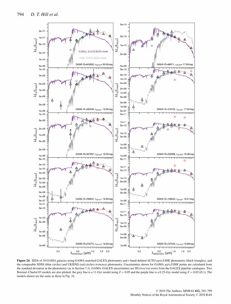
794 D. T. Hill et al.
Figure 24. SEDs of 10 GAMA galaxies using GAMA-matched GALEX photometry and r-band-defined AUTO ugrizYJHK photometry (black triangles), andthe comparable SDSS (blue circles) and UKIDSS (red circles) PETROMAG photometry. Uncertainties shown for GAMA ugrizYJHK points are calculated fromthe standard deviation in the photometry (as in Section 7.3). GAMA–GALEX uncertainties are SEXTRACTOR errors from the GALEX pipeline catalogues. TwoBruzual–Charlot 03 models are also plotted: the grey line is a 11-Gyr model using Z = 0.05 and the purple line is a 0.25-Gyr model using Z = 0.02 (Z�). Themodels shown are the same as those in Fig. 16.
C© 2010 The Authors, MNRAS 412, 765–799Monthly Notices of the Royal Astronomical Society C© 2010 RAS
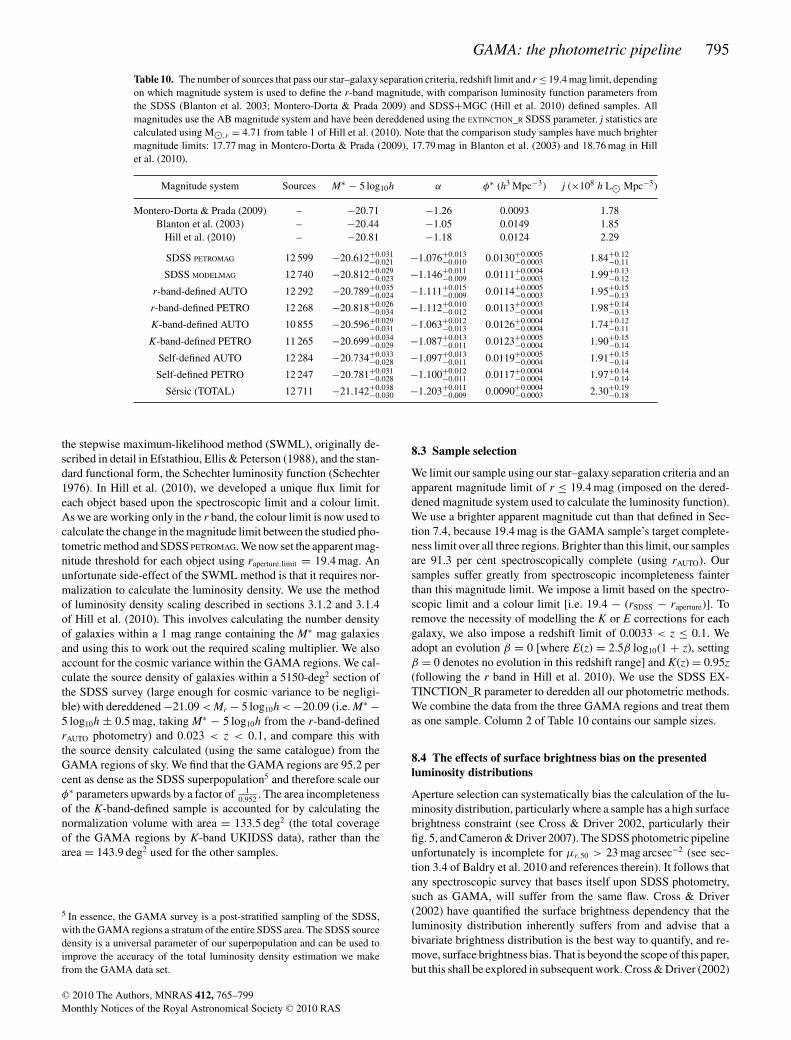
GAMA: the photometric pipeline 795
Table 10. The number of sources that pass our star–galaxy separation criteria, redshift limit and r ≤ 19.4 mag limit, dependingon which magnitude system is used to define the r-band magnitude, with comparison luminosity function parameters fromthe SDSS (Blanton et al. 2003; Montero-Dorta & Prada 2009) and SDSS+MGC (Hill et al. 2010) defined samples. Allmagnitudes use the AB magnitude system and have been dereddened using the EXTINCTION_R SDSS parameter. j statistics arecalculated using M�,r = 4.71 from table 1 of Hill et al. (2010). Note that the comparison study samples have much brightermagnitude limits: 17.77 mag in Montero-Dorta & Prada (2009), 17.79 mag in Blanton et al. (2003) and 18.76 mag in Hillet al. (2010).
Magnitude system Sources M∗ − 5 log10h α φ∗ (h3 Mpc−3) j (×108 h L� Mpc−3)
Montero-Dorta & Prada (2009) – −20.71 −1.26 0.0093 1.78Blanton et al. (2003) – −20.44 −1.05 0.0149 1.85
Hill et al. (2010) – −20.81 −1.18 0.0124 2.29
SDSS PETROMAG 12 599 −20.612+0.031−0.021 −1.076+0.013
−0.010 0.0130+0.0005−0.0003 1.84+0.12
−0.11
SDSS MODELMAG 12 740 −20.812+0.029−0.023 −1.146+0.011
−0.009 0.0111+0.0004−0.0003 1.99+0.13
−0.12
r-band-defined AUTO 12 292 −20.789+0.035−0.024 −1.111+0.015
−0.009 0.0114+0.0005−0.0003 1.95+0.15
−0.13
r-band-defined PETRO 12 268 −20.818+0.026−0.034 −1.112+0.010
−0.012 0.0113+0.0003−0.0004 1.98+0.14
−0.13
K-band-defined AUTO 10 855 −20.596+0.029−0.031 −1.063+0.012
−0.013 0.0126+0.0004−0.0004 1.74+0.12
−0.11
K-band-defined PETRO 11 265 −20.699+0.034−0.029 −1.087+0.013
−0.011 0.0123+0.0005−0.0004 1.90+0.15
−0.14
Self-defined AUTO 12 284 −20.734+0.033−0.028 −1.097+0.013
−0.011 0.0119+0.0005−0.0004 1.91+0.15
−0.14
Self-defined PETRO 12 247 −20.781+0.031−0.028 −1.100+0.012
−0.011 0.0117+0.0004−0.0004 1.97+0.14
−0.14
Sersic (TOTAL) 12 711 −21.142+0.038−0.030 −1.203+0.011
−0.009 0.0090+0.0004−0.0003 2.30+0.19
−0.18
the stepwise maximum-likelihood method (SWML), originally de-scribed in detail in Efstathiou, Ellis & Peterson (1988), and the stan-dard functional form, the Schechter luminosity function (Schechter1976). In Hill et al. (2010), we developed a unique flux limit foreach object based upon the spectroscopic limit and a colour limit.As we are working only in the r band, the colour limit is now used tocalculate the change in the magnitude limit between the studied pho-tometric method and SDSS PETROMAG. We now set the apparent mag-nitude threshold for each object using raperture,limit = 19.4 mag. Anunfortunate side-effect of the SWML method is that it requires nor-malization to calculate the luminosity density. We use the methodof luminosity density scaling described in sections 3.1.2 and 3.1.4of Hill et al. (2010). This involves calculating the number densityof galaxies within a 1 mag range containing the M∗ mag galaxiesand using this to work out the required scaling multiplier. We alsoaccount for the cosmic variance within the GAMA regions. We cal-culate the source density of galaxies within a 5150-deg2 section ofthe SDSS survey (large enough for cosmic variance to be negligi-ble) with dereddened −21.09 < Mr − 5 log10h < −20.09 (i.e. M∗ −5 log10h ± 0.5 mag, taking M∗ − 5 log10h from the r-band-definedrAUTO photometry) and 0.023 < z < 0.1, and compare this withthe source density calculated (using the same catalogue) from theGAMA regions of sky. We find that the GAMA regions are 95.2 percent as dense as the SDSS superpopulation5 and therefore scale ourφ∗ parameters upwards by a factor of 1
0.952 . The area incompletenessof the K-band-defined sample is accounted for by calculating thenormalization volume with area = 133.5 deg2 (the total coverageof the GAMA regions by K-band UKIDSS data), rather than thearea = 143.9 deg2 used for the other samples.
5 In essence, the GAMA survey is a post-stratified sampling of the SDSS,with the GAMA regions a stratum of the entire SDSS area. The SDSS sourcedensity is a universal parameter of our superpopulation and can be used toimprove the accuracy of the total luminosity density estimation we makefrom the GAMA data set.
8.3 Sample selection
We limit our sample using our star–galaxy separation criteria and anapparent magnitude limit of r ≤ 19.4 mag (imposed on the dered-dened magnitude system used to calculate the luminosity function).We use a brighter apparent magnitude cut than that defined in Sec-tion 7.4, because 19.4 mag is the GAMA sample’s target complete-ness limit over all three regions. Brighter than this limit, our samplesare 91.3 per cent spectroscopically complete (using rAUTO). Oursamples suffer greatly from spectroscopic incompleteness fainterthan this magnitude limit. We impose a limit based on the spectro-scopic limit and a colour limit [i.e. 19.4 − (rSDSS − raperture)]. Toremove the necessity of modelling the K or E corrections for eachgalaxy, we also impose a redshift limit of 0.0033 < z ≤ 0.1. Weadopt an evolution β = 0 [where E(z) = 2.5β log10(1 + z), settingβ = 0 denotes no evolution in this redshift range] and K(z) = 0.95z(following the r band in Hill et al. 2010). We use the SDSS EX-TINCTION_R parameter to deredden all our photometric methods.We combine the data from the three GAMA regions and treat themas one sample. Column 2 of Table 10 contains our sample sizes.
8.4 The effects of surface brightness bias on the presentedluminosity distributions
Aperture selection can systematically bias the calculation of the lu-minosity distribution, particularly where a sample has a high surfacebrightness constraint (see Cross & Driver 2002, particularly theirfig. 5, and Cameron & Driver 2007). The SDSS photometric pipelineunfortunately is incomplete for μr,50 > 23 mag arcsec−2 (see sec-tion 3.4 of Baldry et al. 2010 and references therein). It follows thatany spectroscopic survey that bases itself upon SDSS photometry,such as GAMA, will suffer from the same flaw. Cross & Driver(2002) have quantified the surface brightness dependency that theluminosity distribution inherently suffers from and advise that abivariate brightness distribution is the best way to quantify, and re-move, surface brightness bias. That is beyond the scope of this paper,but this shall be explored in subsequent work. Cross & Driver (2002)
C© 2010 The Authors, MNRAS 412, 765–799Monthly Notices of the Royal Astronomical Society C© 2010 RAS

796 D. T. Hill et al.
point out that a sample that is complete to μlim ≥ 24 mag arcsec−2
has very little uncertainty in its Schechter parameters due to sur-face brightness selection effects, as the L∗ population that definethe fitting are fully covered (see also section 4.1.2 of Driver et al.2005). VST KIDS should provide such a catalogue. For now, how-ever, we accept that the SDSS input catalogue will not contain allfaint, low surface brightness galaxies. The luminosity functions wepresent in this section are for samples that are surface brightnesscomplete to μr,50 < 23 mag arcsec−2 and suffer from varying levelsof completeness between 23 < μr,50 < 26 mag arcsec−2. Althoughthese luminosity functions are for a specifically low redshift sample,however, the effects of the surface brightness selection bias shouldbe minimized.
8.5 The effects of the aperture definition system on outputSchechter parameters
Fig. 25 shows the luminosity distributions generated from differ-ent aperture systems and illustrates how dependent the best-fittingluminosity function parameters are on the choice of aperture defini-tion. The best-fitting Schechter function parameters (calculated viaχ 2 minimization) are shown in Table 10.
The proximity of the r-band- and self-defined magnitude lu-minosity distributions signifies that changing the SEXTRACTOR de-
tection threshold (these catalogues utilize a detection threshold of1.7 and 1σ , respectively) has a limited effect on the properties ofa large sample (M∗ − 5 log10h ± 0.055 mag, α ± 0.014, φ∗ ±0.0005 h3 Mpc−3). There is an offset between the K-band and r-band-defined best-fitting luminosity functions. This is not causedby the cosmic variance in the missing area of the K-band sample; thebest-fitting Schechter function parameters vary only slightly whenthis is accounted for. By using the COVER_BITWISE flag, we candefine a population of galaxies that are covered by K-band imaging.The best-fitting Schechter parameters for an rAUTO sample withinan area covered by K-band imaging (and normalized to the smallervolume) are M∗ − 5 log10 h = −20.791 mag, α = −1.115 and φ∗ =0.0114 h3 Mpc−3 – consistent with the area-complete luminosityfunction within the uncertainty. It may be caused by a systematicalteration in the definition of the apertures used to calculate the fluxof the galaxy population.
The best-fitting elliptical Kron and Petrosian aperture luminosityfunctions are similarly distributed in the r-, K- and self-defined sam-ples, indicating that the choice of light-distribution-defined aper-ture does produce an offset that can be quantified. Whether theaperture is circular or elliptical is important. The SDSS PETROMAG
luminosity distribution should be similar to the r-band and self-defined elliptical PETRO distributions, but there is a notable M∗ −5 log10 h offset (0.20 mag; inset of Fig. 25). There is also a marked
-22 -20 -18 -16 -14-5
-4
-3
-2
Figure 25. Luminosity distributions, and the best-fitting Schechter functions, calculated using different aperture definitions. Inset: 1σ chi-squared best-fittingcontours in the M∗–α plane. Errors on luminosity distribution points are Poissonian errors.
C© 2010 The Authors, MNRAS 412, 765–799Monthly Notices of the Royal Astronomical Society C© 2010 RAS

GAMA: the photometric pipeline 797
discrepancy between luminosity distributions calculated using to-tal magnitude apertures (Sersic and SDSS MODELMAG) and light-distribution-defined apertures. The luminosity distributions of theformer are overdense for faint galaxies (Mr − 5 log10 h ≥ −16) andtheir best-fitting power-law slopes are thus flatter.
The Sersic luminosity distribution also measures higher densi-ties of the brightest galaxies. This result is real; we have visuallyinspected the 139 galaxies that are distributed in the −22 ≤ Mr −5 log10 h ≤ −21.5 magnitude bin and only two have suffered catas-trophic failures.6 The remainder are generally well fitted, thoughprominent spiral features do pose difficulties for the fitting algo-rithm. Of the 527 galaxies with Mr,Sersic − 5 log10 h < −21 magwithin our redshift-limited, apparent magnitude cut sample, onlyeight have mr,SDSS − mr,Sersic > 0. The marked discrepancy betweenthe Sersic M∗ − 5 log10h parameter and that generated with theother samples (0.33 mag brighter) is indicative of a scenario wheregalaxies are moved out of the magnitude bins near M∗ − 5 log10 hand into the brighter bins. M∗ is not an independent parameter; itis correlated with the other Schechter parameters and accordinglythe φ∗ parameter has declined. The total luminosity density (j inTable 10), whilst 15 per cent higher, is consistent with that gen-erated by the SDSS model magnitude within uncertainties. As ourSersic magnitudes are not truncated, and the SDSS model magni-tudes are truncated at 7Re for a de Vaucolouers profile and 3Re for anelliptical profile, the M∗ offset between these photometric systems isexpected. We note that the residuals generated by this Sersic-fittingprocess expose the requirement of multicomponent galaxy decom-position; many galaxies have some structure within their centralbulges that the Sersic pipeline cannot model. A multicomponentextension to this pipeline is detailed in Kelvin et al. (2010) andthat paper also examines any discrepancies between the Sersic andmultiple-component fitting results. No matter which aperture sys-tem we use, the luminosity distribution is overdense in the Mr −5 log10 h > −16 magnitude bins when compared to the best-fittingluminosity function. This indicates an upturn in the space densityof galaxies at the dwarf-giant boundary and the limitations of thesingle Schechter function fit.
As noted in the Introduction, the Schechter parameters generatedare for a sample that will suffer surface brightness incompletenessfainter than μ = 23 mag arcsec−2. In a future paper, we intend to ac-count for this effect by undertaking a complete bivariate brightnessanalysis of the sample. The total luminosity densities we show heremay therefore be systematically underdense due to surface bright-ness limitations (cf. Cross & Driver 2002). It is also apparent thatthe simple Schechter function parametrization is no longer a goodfit for the luminosity distribution of galaxies at fainter magnitudes;there is an obvious upturn in each sample that is not being modelled.As the Sersic photometric system is the only system that accountsfor missing light, it is the most effective way of calculating theluminosity distribution.
9 SU M M A RY
The GAMA photometric pipeline has been designed to combinephotometric data from a number of sources in a scientific and con-sistent manner. We have generated a series of large mosaics fromimaging data taken from the SDSS and UKIDSS instruments usingthe SWARP utility and undertaken optical and NIR photometry on an
6 These profiles are viewable at http://star-www.st-and.ac.uk/∼dth4/139eye/
r- and K-band-defined sample of sources using SEXTRACTOR. Wehave also used a GALFIT-based pipeline (SIGMA) to generate SersicugrizYJHK magnitudes for all sources within the GAMA samplethat pass our star–galaxy separation criteria.
We have created a set of r-band-defined source catalogues in theugrizYJHK passbands, calculated the apparent magnitude limits atwhich these samples are complete and estimated their current red-shift completeness. Whilst these samples do not contain as manysources as those used to calculate the SDSS luminosity functions(Blanton et al. 2003; Montero-Dorta & Prada 2009), they are com-plete to a greater depth. Our NIR apparent-magnitude-limited cat-alogues are of comparable size to those produced by the 6dFGS(Jones et al. 2009), with the decrease in coverage area matched byincreasing depth. Our source catalogues have the advantage that theycan be used to accurately compare the optical and NIR luminosityof any source within our sample. As the aperture definition is con-stant, we can calculate exact colours. We have attempted to quantifythe level of uncertainty in source flux due to the definition of theaperture. We find that the uncertainty is generally ∼400 per cent ofthe SEXTRACTOR output uncertainty (produced by background noisevariations and signal-to-noise ratio).
We have attempted to quantify the percentage of mismatchesbetween our catalogues and the SDSS catalogues. We have takena subset region of our images and tested their results against theSDSS detection software. We have detailed reasons for mismatchesbetween these catalogues. They are generally an issue of differentdeblending decisions, artefacts, background noise or proximity tosaturated stars. We find that there do seem to be some low surfacebrightness, compact objects that are missed by the SDSS detec-tion software and are found by SEXTRACTOR, and some false SDSSdetections. These faulty sources would be removed from the spec-troscopic observing list by the extensive visual classification processundertaken by the GAMA team.
As our Sersic magnitudes are generated from the images thatthe profile is calculated on, the colours produced from the Sersicmagnitudes are liable to be inaccurate and suffer from bias due tothe aperture definition. We have defined a set of ‘fixed-aperture’Sersic magnitudes using the Sersic r-band magnitude and coloursfrom the r-band-defined AUTO catalogue. We recommend the useof these magnitudes, called Xtotal. These magnitudes will provideboth an accurate estimate of the luminosity of each galaxy andoptimal colours.
The GAMA photometric pipeline catalogue does not have thebreadth of focus that the existing products from the SDSS andUKIDSS surveys have. As both the instrument gain (in SDSS only)and seeing change from frame to frame, our mosaics have variationswithin them that would cause errors in the calculation of stellarphotometry. We have not attempted to deal with saturated objects,which causes uncertainty at the bright end of our catalogue, ormasking of artefacts. These problems primarily affect stars and areremoved following the extensive visual classification programmewe have undertaken. For the task our catalogues were developed, theaccurate calculation of extended source apertures across instrumentsfor a specific sample of extended sources, they are more adept thanthe existing tools.
Finally, we have generated r-band luminosity distributions andbest-fitting luminosity functions from our population of galaxies us-ing nine different aperture definitions: SDSS circular Petrosian andModel magnitudes, r-band-defined elliptical Petrosian and AUTOmagnitudes, K-band-defined elliptical Petrosian and AUTO magni-tudes, self-defined elliptical Petrosian and AUTO magnitudes, andan elliptical Sersic total magnitude. We find that the r-band and
C© 2010 The Authors, MNRAS 412, 765–799Monthly Notices of the Royal Astronomical Society C© 2010 RAS

798 D. T. Hill et al.
self-defined elliptical, light-distribution-defined apertures producesimilar results, indicating that the choice of detection threshold isunimportant. We find that there is a similar AUTO–PETRO offset inthe r-band, self- and K-band-defined samples. We find that the useof circular apertures does have an effect on the best-fitting Schechterfit, with the SDSS PETROMAG having a fainter M∗ parameter than theSEXTRACTOR samples. We also find that the use of total magnitudesystems affects the slope of the luminosity function, with both theSersic and SDSS MODELMAG luminosity functions having a steeperα parameter. When we calculate the total luminosity density foreach sample, we find that using the Sersic magnitude system givesus a higher value, approximately 15 per cent higher than samplesthat use other aperture definition systems. Following visual clas-sification of a subsection of our sample, it is clear that this is notdue to errors within our Sersic magnitude calculation. We also notethat the Schechter luminosity function does not provide a good fitat the faint end of the luminosity distribution and a clear upturn atthe dwarf-giant boundary is seen.
AC K N OW L E D G M E N T S
DTH and LSK are funded by STFC studentships. ASGR is fundedby a STFC grant. AMH acknowledges support provided by the Aus-tralian Research Council through a QEII Fellowship (DP0557850).
Funding for the SDSS and SDSS-II has been provided by the Al-fred P. Sloan Foundation, the Participating Institutions, the NationalScience Foundation, the US Department of Energy, the NationalAeronautics and Space Administration, the Japanese Monbuka-gakusho, the Max Planck Society, and the Higher Education Fund-ing Council for England. The SDSS website is http://www.sdss.org/.The SDSS is managed by the Astrophysical Research Consortiumfor the Participating Institutions. The Participating Institutions arethe American Museum of Natural History, Astrophysical InstitutePotsdam, University of Basel, University of Cambridge, Case West-ern Reserve University, University of Chicago, Drexel University,Fermilab, the Institute for Advanced Study, the Japan ParticipationGroup, Johns Hopkins University, the Joint Institute for Nuclear As-trophysics, the Kavli Institute for Particle Astrophysics and Cosmol-ogy, the Korean Scientist Group, the Chinese Academy of Sciences(LAMOST), Los Alamos National Laboratory, the Max-Planck-Institute for Astronomy (MPIA), the Max-Planck-Institute for As-trophysics (MPA), New Mexico State University, Ohio State Univer-sity, University of Pittsburgh, University of Portsmouth, PrincetonUniversity, the United States Naval Observatory, and the Universityof Washington.
The UKIDSS project is defined in Lawrence et al. (2007). TheUKIDSS uses the UKIRT Wide Field Camera (WFCAM; Casaliet al. 2007) and a photometric system described in Hewett et al.(2006). The pipeline processing and science archive are describedin Irwin et al (in preparation) and Hambly et al. (2008).
STILTS is a set of command-line-based catalogue matchingtools, based upon the STIL library. It is currently being sup-ported by its author (Mark Taylor) and can be downloaded fromhttp://www.star.bris.ac.uk/∼mbt/stilts/.
We thank Robert Lupton for his useful comments and suggestionswhen refereeing this paper.
RE FER ENCES
Abazajian K. et al., 2004, AJ, 128, 502Adelman-McCarthy J. K. et al., 2008, ApJS, 175, 297Andreon S., 2002, A&A, 382, 495
Baldry I. K. et al., 2010, MNRAS, 404, 86Bertin E., Arnouts S., 1996, A&AS, 117, 393Bertin E., Mellier Y., Radovich M., Missonnier G., Didelon P., Morin B.,
2002, in Bohlender D. A., Durand D., Handley T. H., eds, ASP Conf.Ser. Vol. 281, Astronomical Data Analysis Software and Systems XI,The TERAPIX Pipeline. Astron. Soc. Pac., San Francisco, p. 228
Blanton M. R. et al., 2003, ApJ, 592, 819Brown R. J. N. et al., 2003, MNRAS, 341, 747Bruzual G., Charlot S., 2003, MNRAS, 344, 1000Cameron E., Driver S. P., 2007, MNRAS, 377, 523Caon N., Capaccioli M., Rampazzo R., 1990, A&AS, 86, 429Casali M. et al., 2007, A&A, 467, 777Chabrier G., 2003, PASP, 115, 763Cohen M., Wheaton W. A., Megeath S. T., 2003, AJ, 126, 1090Cross N., Driver S. P., 2002, MNRAS, 329, 579de Vaucouleurs G., 1948, Ann. Astrophys., 11, 247Driver S. P., Liske J., Cross N. J. G., De Propris R., Allen P. D., 2005,
MNRAS, 360, 81Driver S. P. et al., 2009, Astron. Geophys., 50, 050000Driver S. P. et al., 2010, preprint (arXiv:1009.0614)Eales S. et al., 2010, PASP, 122, 499Efstathiou G., Ellis R. S., Peterson B. A., 1988, MNRAS, 232, 431Freeman K. C., 1970, ApJ, 160, 811Graham A. W., 2001, AJ, 121, 820Graham A. W., Driver S. P., 2005, PASA, 22, 118Graham A. W., Driver S. P., Petrosian V., Conselice C. J., Bershady M. A.,
Crawford S. M., Goto T., 2005, AJ, 130, 1535Hambly N. C. et al., 2008, MNRAS, 384, 637Hewett P. C., Warren S. J., Leggett S. K., Hodgkin S. T., 2006, MNRAS,
367, 454Hill D. T., Driver S. P., Cameron E., Cross N., Liske J., Robotham A., 2010,
MNRAS, 404, 1215Høg E. et al., 2000, A&A, 355, L27Ivezic Z et al., 2004, Astron. Nachr., 325, 583Jones D. H. et al., 2009, MNRAS, 399, 683Kelvin L., Driver S., Robotham A., Hill D., Cameron E., 2010, in Debattista
V. P., Popescu C. C., eds., AIP Conf. Ser. Vol. 1240, Exploring. GalaxyFormation and Evolution via Structural Decomposition. Am. Inst. Phys.,New York, p. 247
Kron R. G., 1980, ApJS, 43, 305Lawrence A. et al., 2007, MNRAS, 379, 1599Montero-Dorta A. D., Prada F., 2009, MNRAS, 399, 1106Patterson F. S., 1940, Harvard College Obser. Bull., 914, 9Peng C. Y., Ho L. C., Impey C. D., Rix H. W., 2007, BAAS, 38, 804Petrosian V., 1976, ApJ, 209, L1Pier J. R. et al., 2003, AJ, 125, 1559Robotham A. et al., 2010, PASA, 27, 76Schechter P., 1976, ApJ, 203, 297Sersic J. L., 1963, Bol. Asoc. Argentina de Astron. La Plata Argentina, 6,
41Smith A. J., Loveday J., Cross N. J. G., 2009, MNRAS, 397, 868Stoughton C. et al., 2002, AJ, 123, 485Strauss M. A. et al., 2002, AJ, 124, 1810Taylor M. B., 2006, in Gabriel C., Arviset C., Ponz D., Enrique S., eds, ASP
Conf. Ser. Vol. 351, STILTS - A Package for Command-Line Processingof Tabular Data. Astron. Soc. Pac., San Francisco, p. 666
Warren S. J. et al., 2007, MNRAS, 375, 213Willmer C. N. A., 1997, AJ, 114, 898Wyder T. K. et al., 2005, ApJ, 619, L15York D. G. et al., 2000, AJ, 120, 1579Zacharias N. et al., 2000, AJ, 120, 2131
APPENDI X A : VARI ATI ON BETWEENPA SSBANDS
Fig. A1 shows the 18 200 × 200 pixel images of the piece of skycontaining SDSS object 588848900968480848, nine cut-outs from
C© 2010 The Authors, MNRAS 412, 765–799Monthly Notices of the Royal Astronomical Society C© 2010 RAS

GAMA: the photometric pipeline 799
Figure A1. The effects of convolution and the change in passband of observations of SDSS object 588848900968480848.
the standard image mosaics and nine from the convolved imagemosaics. What is easily notable is that not only does the abilityto see features of the object changes dramatically between the u(top left-hand panel) and K (bottom right-hand panel) wavebands(spiral arms are visible in the optical, but in the K band, there onlyseems to be a bar and a bulge component), but also objects aroundit appear and disappear (a small blip to the south-east in the r bandthat may or may not be part of the object itself, at least five faintobjects to the east of the frame in the NIR). The size of the objectseems to halve from the g band to the J band, though this maybe an effect of the image quality (the SDSS g band should havea much smoother background than the UKIDSS J). The apparentmagnitude of the object itself changes by 2.8 mag from u to itspeak in H (SEXTRACTOR calculates AB magnitudes using an r-band-
defined AUTO aperture of 16.67, 15.44, 14.85, 14.49, 14.32, 14.23,14.04, 13.83 and 14.11 mag in ugrizYJHK). This is probably due tothe decrease in dust opacity from the UV to the NIR.
The convolved images also show greater variation between theobject and the background (these images all use a linear scale be-tween the 99.5 per cent quantile pixel and 0, the background). Forinstance, the extended spiral arm to the left-hand side of the bulge inthe u band becomes slightly more apparent in the convolved u-bandimage. The size of the object in the convolved images generallylooks larger than the standard images, though this again is probablydue to the smoothing of the background, making flux overdensitiesmore apparent in the convolved images.
This paper has been typeset from a TEX/LATEX file prepared by the author.
C© 2010 The Authors, MNRAS 412, 765–799Monthly Notices of the Royal Astronomical Society C© 2010 RAS