g – 1 copyright © 2010 pearson education, inc. publishing as prentice hall. acceptance sampling...
TRANSCRIPT

G – 1Copyright © 2010 Pearson Education, Inc. Publishing as Prentice Hall.
Acceptance Sampling PlansAcceptance Sampling PlansG
For For Operations Management, 9eOperations Management, 9e by by Krajewski/Ritzman/Malhotra Krajewski/Ritzman/Malhotra © 2010 Pearson Education© 2010 Pearson Education
PowerPoint Slides PowerPoint Slides by Jeff Heylby Jeff Heyl
AQL LTPD
G – 2Copyright © 2010 Pearson Education, Inc. Publishing as Prentice Hall.
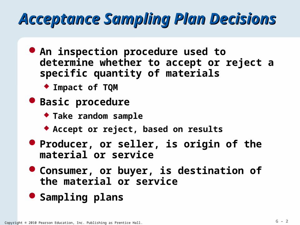
Acceptance Sampling Plan Acceptance Sampling Plan Decisions Decisions
An inspection procedure used to determine whether to accept or reject a specific quantity of materials Impact of TQM
Basic procedure Take random sample Accept or reject, based on results
Producer, or seller, is origin of the material or service
Consumer, or buyer, is destination of the material or service
Sampling plans
G – 3Copyright © 2010 Pearson Education, Inc. Publishing as Prentice Hall.
Quality and Risk DecisionsQuality and Risk Decisions
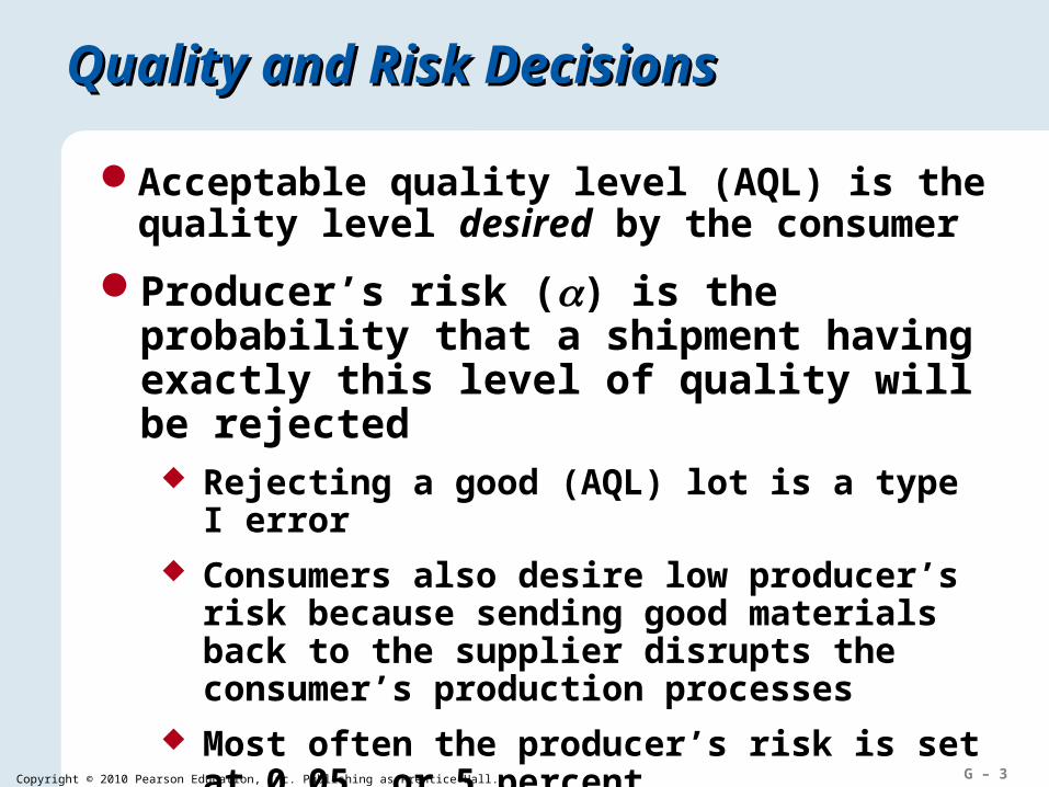
Acceptable quality level (AQL) is the quality level desired by the consumer
Producer’s risk () is the probability that a shipment having exactly this level of quality will be rejected
Rejecting a good (AQL) lot is a type I error Consumers also desire low producer’s risk
because sending good materials back to the supplier disrupts the consumer’s production processes
Most often the producer’s risk is set at 0.05, or 5 percent

G – 4Copyright © 2010 Pearson Education, Inc. Publishing as Prentice Hall.
Quality and Risk DecisionsQuality and Risk Decisions
Lot tolerance proportion defective (LTPD), the worst level the customer can tolerate
Consumer’s risk, ( ) is the probability a shipment having exactly this level of quality (the LTPD) will be accepted
Accepting a bad (LTPD) lot is a type II error A common value for the consumer’s risk is
0.10, or 10 percent
G – 5Copyright © 2010 Pearson Education, Inc. Publishing as Prentice Hall.
Single-Sampling PlansSingle-Sampling Plans
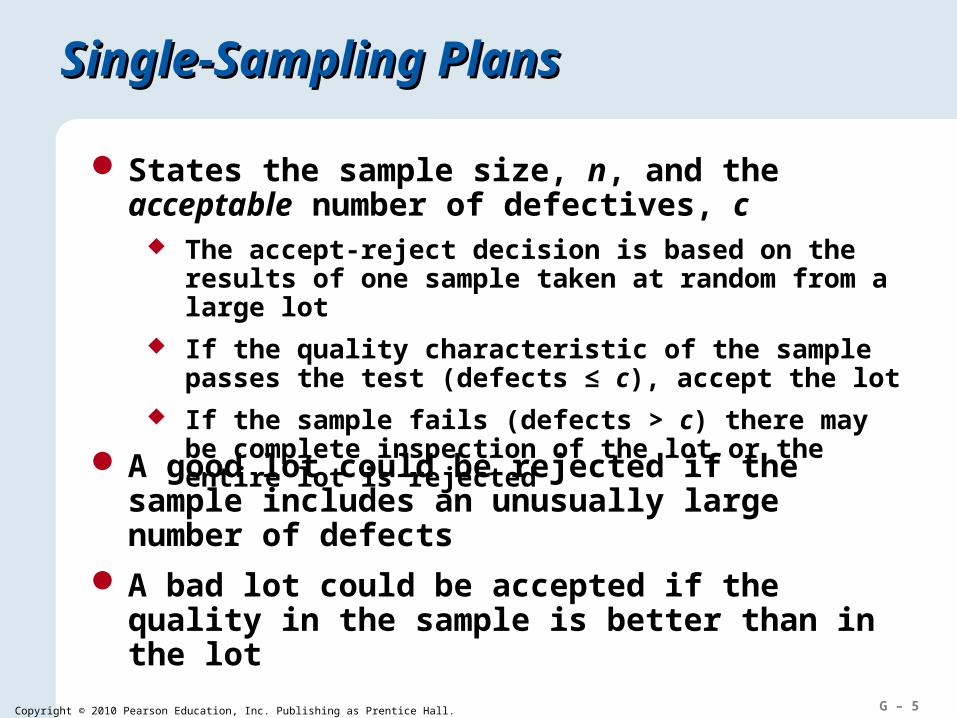
States the sample size, n, and the acceptable number of defectives, c
The accept-reject decision is based on the results of one sample taken at random from a large lot
If the quality characteristic of the sample passes the test (defects ≤ c), accept the lot
If the sample fails (defects > c) there may be complete inspection of the lot or the entire lot is rejected
A good lot could be rejected if the sample includes an unusually large number of defects
A bad lot could be accepted if the quality in the sample is better than in the lot

G – 6Copyright © 2010 Pearson Education, Inc. Publishing as Prentice Hall.
Double-Sampling PlansDouble-Sampling Plans
Two sample sizes, (n1 and n2), and two acceptance numbers (c1 and c2)
Take a random sample of relatively small size n1, from a large lot
If the sample passes the test (≤ c1), accept the lot
If the sample fails (> c2), the entire lot is rejected
If the sample is between c1 and c2, then take a larger second random sample, n2
If the combined number of defects ≤ c2 accept the lot, otherwise reject

G – 7Copyright © 2010 Pearson Education, Inc. Publishing as Prentice Hall.
Sequential Sampling PlansSequential Sampling Plans
Results of random samples of one unit, tested one-by-one, are compared to sequential-sampling chart
Chart guides decision to reject, accept, or continue sampling, based on cumulative results
Average number of items inspected (ANI) is generally lower with sequential sampling

G – 8Copyright © 2010 Pearson Education, Inc. Publishing as Prentice Hall.
Reject
Continue sampling
Accept
8 –
7 –
6 –
5 –
4 –
3 –
2 –
1 –
0 –
Cumulative sample size
| | | | | | |
10 20 30 40 50 60 70
Nu
mb
er
of
de
fec
tiv
es
Sequential Sampling ChartSequential Sampling Chart
Figure G.1 – Sequential-Sampling Chart

G – 9Copyright © 2010 Pearson Education, Inc. Publishing as Prentice Hall.
Operating Characteristic Curve Operating Characteristic Curve
Perfect discrimination between good and bad lots requires 100% inspection
Select sample size n and acceptance number c to achieve the level of performance specified by the AQL, , LTPD, and
Drawing the OC curve
The OC curve shows the probability of accepting a lot Pa, as a dependent function of p, the true proportion of defectives in the lot
For every possible combination of n and c, there exists a unique operating characteristics curve

G – 10Copyright © 2010 Pearson Education, Inc. Publishing as Prentice Hall.
Operating Characteristic CurveOperating Characteristic Curve
Ideal OC curve
Typical OC curve
1.0
AQL LTPD
Pro
bab
ilit
y o
f ac
cep
tan
ce
Proportion defective
Figure G.2 – Operating Characteristic Curves
G – 11Copyright © 2010 Pearson Education, Inc. Publishing as Prentice Hall.
Constructing an OC CurveConstructing an OC Curve
EXAMPLE G.1
The Noise King Muffler Shop, a high-volume installer of replacement exhaust muffler systems, just received a shipment of 1,000 mufflers. The sampling plan for inspecting these mufflers calls for a sample size n = 60 and an acceptance number c = 1. The contract with the muffler manufacturer calls for an AQL of 1 defective muffler per 100 and an LTPD of 6 defective mufflers per 100. Calculate the OC curve for this plan, and determine the producer’s risk and the consumer’s risk for the plan.

G – 12Copyright © 2010 Pearson Education, Inc. Publishing as Prentice Hall.
Constructing an OC CurveConstructing an OC Curve
SOLUTION
Let p = 0.01. Then multiply n by p to get 60(0.01) = 0.60. Locate 0.60 in Table G.1. Move to the right until you reach the column for c = 1. Read the probability of acceptance: 0.878. Repeat this process for a range of p values. The following table contains the remaining values for the OC curve.
Values for the Operating Characteristic Curve with n = 60 and c = 1
Proportion Defective (p)
npProbability of c or Less Defects (Pa) Comments
0.01 (AQL) 0.6 0.878 = 1.000 – 0.878 = 0.122
0.02 1.2 0.663
0.03 1.8 0.463
0.04 2.4 0.308
0.05 3.0 0.199
0.06 (LTPD) 3.6 0.126 = 0.126
0.07 4.2 0.078
0.08 4.8 0.048
0.09 5.4 0.029
0.10 6.0 0.017

G – 13Copyright © 2010 Pearson Education, Inc. Publishing as Prentice Hall.
Constructing an OC CurveConstructing an OC Curve
0.878
0.663
0.463
0.308
0.1990.126 0.078
0.048 0.0290.017
(AQL) (LTPD)
1.0 –
0.9 –
0.8 –
0.7 –
0.6 –
0.5 –
0.4 –
0.3 –
0.2 –
0.1 –
0.0 – | | | | | | | | | |1 2 3 4 5 6 7 8 9 10
Proportion defective (hundredths)
Pro
bab
ilit
y o
f ac
cep
tan
ce
= 0.126
= 0.122
Figure G.3 – The OC Curve for Single-Sampling Plan with n = 60 and c = 1

G – 14Copyright © 2010 Pearson Education, Inc. Publishing as Prentice Hall.
Application G.1Application G.1
A sampling plan is being evaluated where c = 10 and n = 193. If AQL = 0.03 and LTPD = 0.08. What are the producer’s risk and consumer’s risk for the plan? Draw the OC curve.
SOLUTION
Finding (probability of rejecting AQL quality)
p =
np =
Pa =
=
0.03
5.79
0.965
0.035 (or 1.0 – 0.965)
Finding (probability of accepting LTPD quality)
p =
np =
Pa =
=
0.08
15.44
0.10
0.10

G – 15Copyright © 2010 Pearson Education, Inc. Publishing as Prentice Hall.
Application G.1Application G.1
1.0 –
0.8 –
0.6 –
0.4 –
0.2 –
0.0 –| | | | | | | | | | |
0 2 4 6 8 10
Pro
bab
ility
of
acce
pta
nce
Percentage defective
= 0.035
= 0.10

G – 16Copyright © 2010 Pearson Education, Inc. Publishing as Prentice Hall.
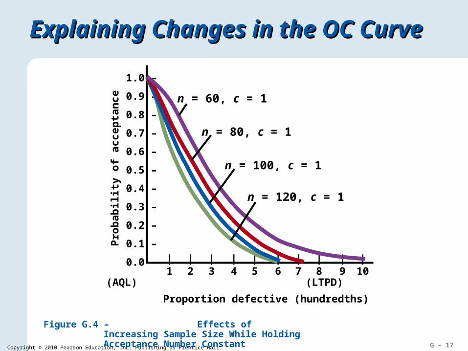
Explaining Changes in the OC CurveExplaining Changes in the OC Curve
Sample size effect Increasing n while holding c constant
increases the producer’s risk and reduces the consumer’s risk
nProducer’s Risk
(p = AQL)Consumer’s Risk
(p = LTPD)
60 0.122 0.126
80 0.191 0.048
100 0.264 0.017
120 0.332 0.006
G – 17Copyright © 2010 Pearson Education, Inc. Publishing as Prentice Hall.
Explaining Changes in the OC CurveExplaining Changes in the OC Curve
1.0 –
0.9 –
0.8 –
0.7 –
0.6 –
0.5 –
0.4 –
0.3 –
0.2 –
0.1 –
0.0 – | | | | | | | | | |1 2 3 4 5 6 7 8 9 10
(AQL) (LTPD)
Proportion defective (hundredths)
Pro
bab
ility
of
acce
pta
nce
n = 60, c = 1
n = 80, c = 1
n = 100, c = 1
n = 120, c = 1
Figure G.4 – Effects of Increasing Sample Size While Holding Acceptance Number Constant
G – 18Copyright © 2010 Pearson Education, Inc. Publishing as Prentice Hall.
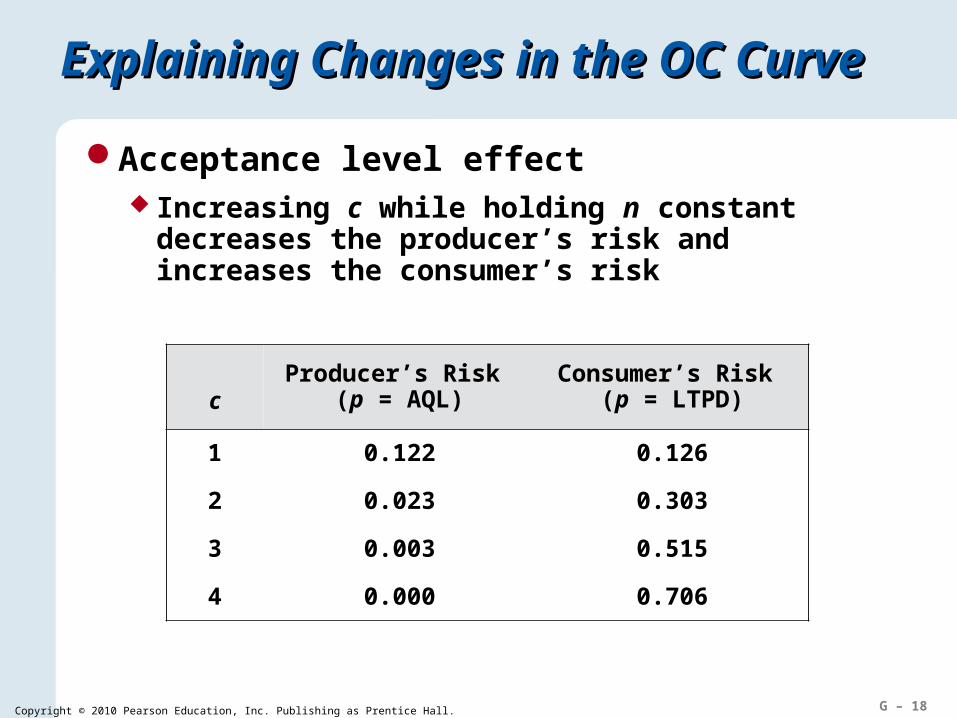
Explaining Changes in the OC CurveExplaining Changes in the OC Curve
Acceptance level effect Increasing c while holding n constant
decreases the producer’s risk and increases the consumer’s risk
cProducer’s Risk
(p = AQL)Consumer’s Risk
(p = LTPD)
1 0.122 0.126
2 0.023 0.303
3 0.003 0.515
4 0.000 0.706

G – 19Copyright © 2010 Pearson Education, Inc. Publishing as Prentice Hall.
Explaining Changes in the OC CurveExplaining Changes in the OC Curve
1.0 –
0.9 –
0.8 –
0.7 –
0.6 –
0.5 –
0.4 –
0.3 –
0.2 –
0.1 –
0.0 – | | | | | | | | | |1 2 3 4 5 6 7 8 9 10
(AQL) (LTPD)
Proportion defective (hundredths)
Pro
bab
ility
of
acce
pta
nce
n = 60, c = 1
n = 60, c = 2
n = 60, c = 3n = 60, c = 4
Figure G.5 – Effects of Increasing Acceptance Number While Holding Sample Size Constant
G – 20Copyright © 2010 Pearson Education, Inc. Publishing as Prentice Hall.
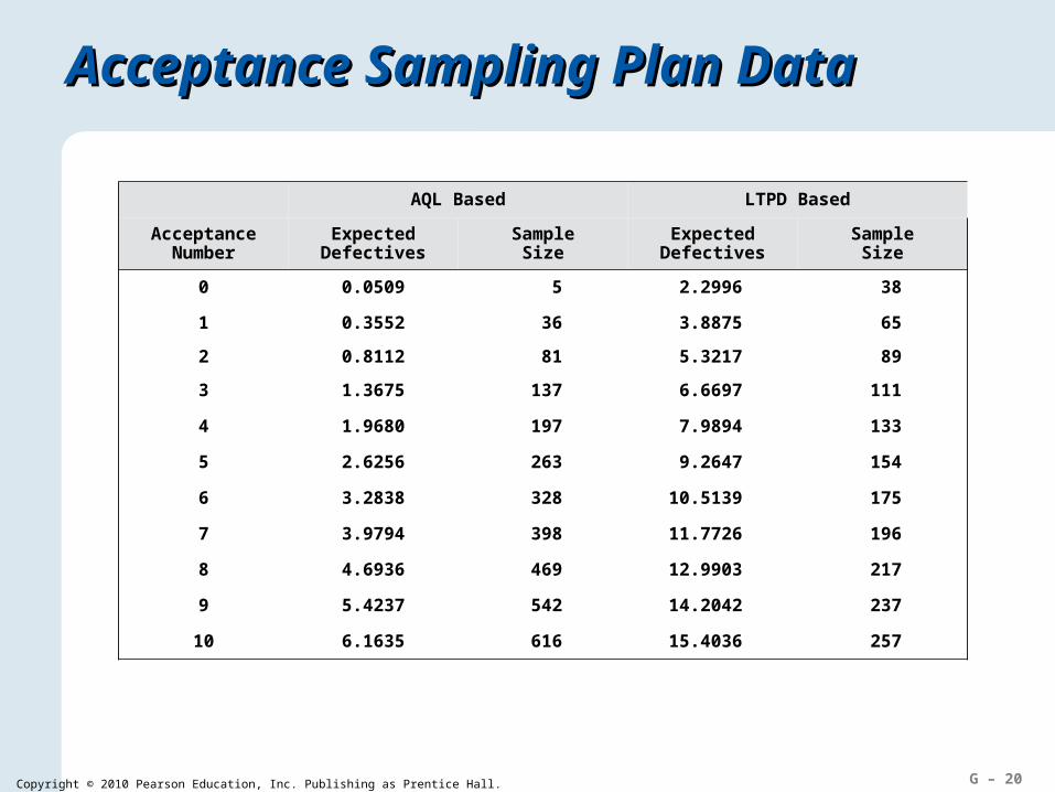
Acceptance Sampling Plan DataAcceptance Sampling Plan Data
AQL Based LTPD Based
Acceptance Number
Expected Defectives
SampleSize
Expected Defectives
SampleSize
0 0.0509 5 2.2996 38
1 0.3552 36 3.8875 65
2 0.8112 81 5.3217 89
3 1.3675 137 6.6697 111
4 1.9680 197 7.9894 133
5 2.6256 263 9.2647 154
6 3.2838 328 10.5139 175
7 3.9794 398 11.7726 196
8 4.6936 469 12.9903 217
9 5.4237 542 14.2042 237
10 6.1635 616 15.4036 257
G – 21Copyright © 2010 Pearson Education, Inc. Publishing as Prentice Hall.
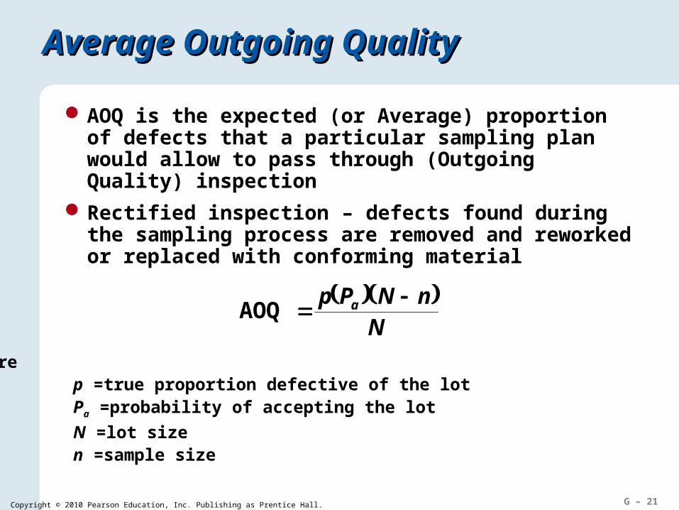
Average Outgoing Quality Average Outgoing Quality
AOQ is the expected (or Average) proportion of defects that a particular sampling plan would allow to pass through (Outgoing Quality) inspection
Rectified inspection – defects found during the sampling process are removed and reworked or replaced with conforming material
N
nNPp a AOQ
wherep =true proportion defective of the lotPa =probability of accepting the lot
N = lot sizen =sample size
G – 22Copyright © 2010 Pearson Education, Inc. Publishing as Prentice Hall.
Average Outgoing Quality Average Outgoing Quality
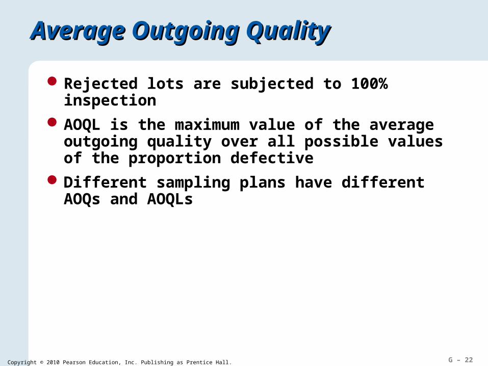
Rejected lots are subjected to 100% inspection
AOQL is the maximum value of the average outgoing quality over all possible values of the proportion defective
Different sampling plans have different AOQs and AOQLs
G – 23Copyright © 2010 Pearson Education, Inc. Publishing as Prentice Hall.
Calculating the AOQLCalculating the AOQL
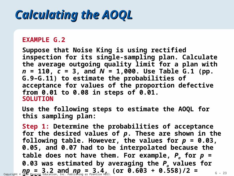
EXAMPLE G.2
Suppose that Noise King is using rectified inspection for its single-sampling plan. Calculate the average outgoing quality limit for a plan with n = 110, c = 3, and N = 1,000. Use Table G.1 (pp. G.9–G.11) to estimate the probabilities of acceptance for values of the proportion defective from 0.01 to 0.08 in steps of 0.01.
SOLUTION
Use the following steps to estimate the AOQL for this sampling plan:
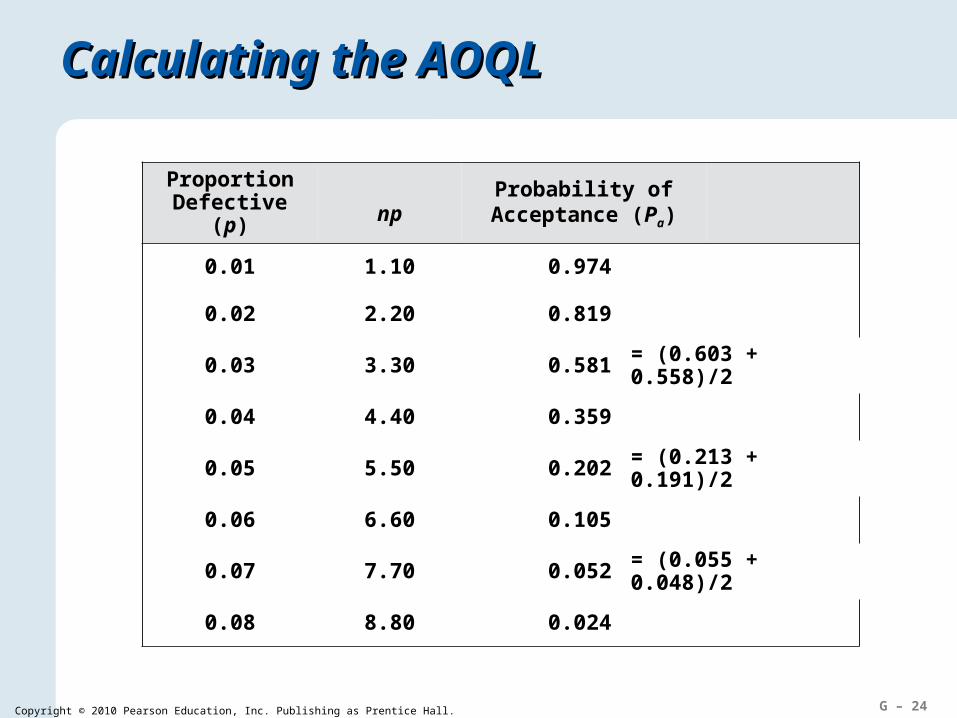
Step 1: Determine the probabilities of acceptance for the desired values of p. These are shown in the following table. However, the values for p = 0.03, 0.05, and 0.07 had to be interpolated because the table does not have them. For example, Pa for p = 0.03 was estimated by averaging the Pa values for np = 3.2 and np = 3.4, (or 0.603 + 0.558)/2 = 0.580.
G – 24Copyright © 2010 Pearson Education, Inc. Publishing as Prentice Hall.
Calculating the AOQLCalculating the AOQL
Proportion Defective (p) np
Probability of Acceptance (Pa)
0.01 1.10 0.974
0.02 2.20 0.819
0.03 3.30 0.581 = (0.603 + 0.558)/2
0.04 4.40 0.359
0.05 5.50 0.202 = (0.213 + 0.191)/2
0.06 6.60 0.105
0.07 7.70 0.052 = (0.055 + 0.048)/2
0.08 8.80 0.024

G – 25Copyright © 2010 Pearson Education, Inc. Publishing as Prentice Hall.
Calculating the AOQLCalculating the AOQL
Step 2: Calculate the AOQ for each value of p.
For p = 0.01: 0.01(0.974)(1000 – 110)/1000 = 0.0087
The plot of the AOQ values is shown in Figure G.6.
For p = 0.02: 0.02(0.819)(1000 – 110)/1000 = 0.0146
For p = 0.03: 0.03(0.581)(1000 – 110)/1000 = 0.0155
For p = 0.04: 0.04(0.359)(1000 – 110)/1000 = 0.0128
For p = 0.05: 0.05(0.202)(1000 – 110)/1000 = 0.0090
For p = 0.06: 0.06(0.105)(1000 – 110)/1000 = 0.0056
For p = 0.07: 0.07(0.052)(1000 – 110)/1000 = 0.0032
For p = 0.08: 0.08(0.024)(1000 – 110)/1000 = 0.0017

G – 26Copyright © 2010 Pearson Education, Inc. Publishing as Prentice Hall.
Calculating the AOQLCalculating the AOQL
Step 3: Identify the largest AOQ value, which is the estimate of the AOQL. In this example, the AOQL is 0.0155 at p = 0.03.
AOQL1.6 –
1.2 –
0.8 –
0.4 –
0 –| | | | | | | |1 2 3 4 5 6 7 8
Defectives in lot (percent)
Ave
rag
e o
utg
oin
g q
ual
ity
(per
cen
t)
Figure G.5 – Average Outgoing Quality Curve for the Noise King Muffler Service

G – 27Copyright © 2010 Pearson Education, Inc. Publishing as Prentice Hall.
Application G.2Application G.2
Demonstrate the model for computing AOQ
Management has selected the following parameters:
AQL = 0.01 = 0.05
LTPD = 0.06 = 0.10
n = 100 c = 3
What is the AOQ if p = 0.05 and N = 3000?
p =
np =
Pa =
AOQ =
0.05
1000(0.05) = 5
0.265
3000
29002650050 ..= 0.0128
SOLUTION
G – 28Copyright © 2010 Pearson Education, Inc. Publishing as Prentice Hall.
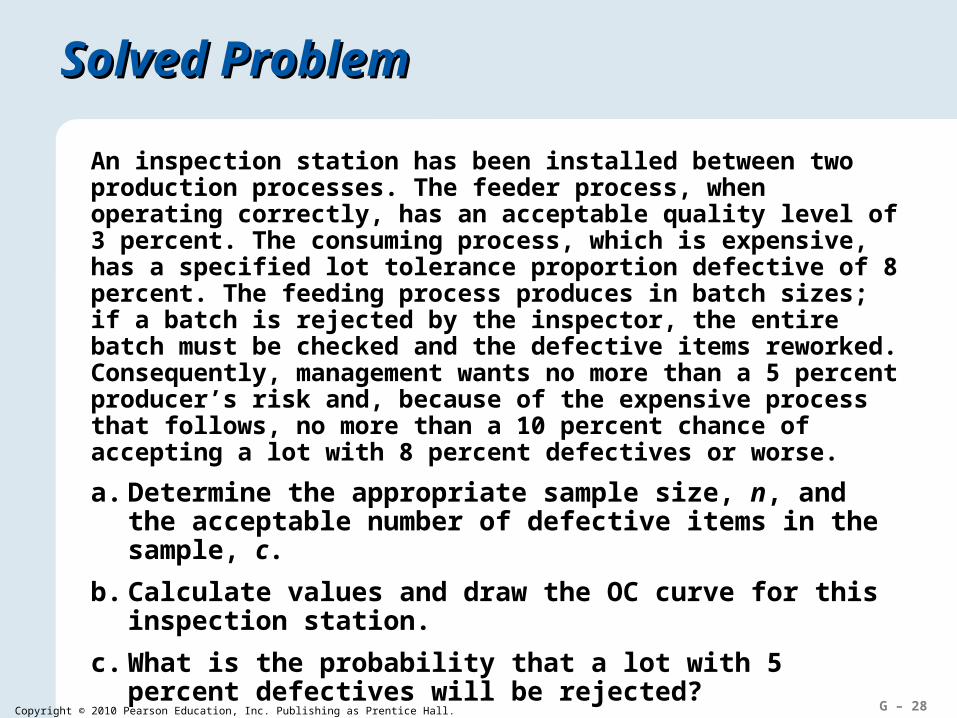
An inspection station has been installed between two production processes. The feeder process, when operating correctly, has an acceptable quality level of 3 percent. The consuming process, which is expensive, has a specified lot tolerance proportion defective of 8 percent. The feeding process produces in batch sizes; if a batch is rejected by the inspector, the entire batch must be checked and the defective items reworked. Consequently, management wants no more than a 5 percent producer’s risk and, because of the expensive process that follows, no more than a 10 percent chance of accepting a lot with 8 percent defectives or worse.
Solved ProblemSolved Problem
a. Determine the appropriate sample size, n, and the acceptable number of defective items in the sample, c.
b. Calculate values and draw the OC curve for this inspection station.
c. What is the probability that a lot with 5 percent defectives will be rejected?

G – 29Copyright © 2010 Pearson Education, Inc. Publishing as Prentice Hall.
Solved ProblemSolved Problem
SOLUTION
a. For AQL = 3 percent, LTPD = 8 percent, = 5 percent, and = 10 percent, use Table G.1 and trial and error to arrive at a sampling plan. If n = 180 and c = 9,
np =
np =
180(0.03) = 5.4
= 0.049
180(0.08) = 14.4
= 0.092
Sampling plans that would also work are n = 200, c = 10; n = 220, c = 10; and n = 240, c = 12.
G – 30Copyright © 2010 Pearson Education, Inc. Publishing as Prentice Hall.
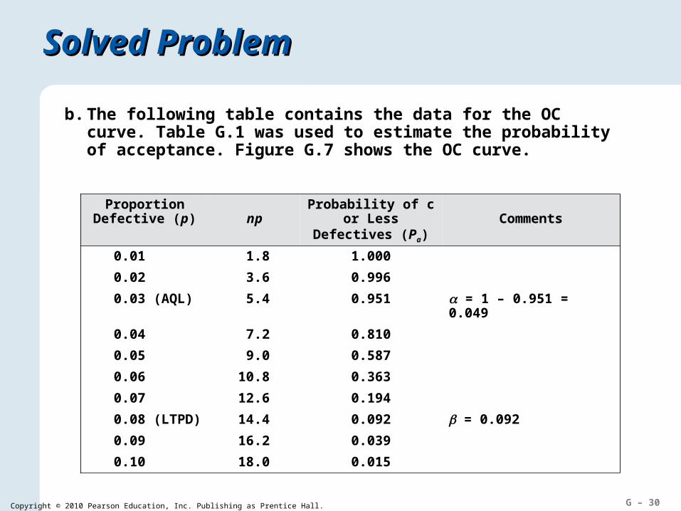
Solved ProblemSolved Problem
b. The following table contains the data for the OC curve. Table G.1 was used to estimate the probability of acceptance. Figure G.7 shows the OC curve.
Proportion Defective (p) np
Probability of c or Less Defectives (Pa) Comments
0.01 1.8 1.000
0.02 3.6 0.996
0.03 (AQL) 5.4 0.951 = 1 – 0.951 = 0.049
0.04 7.2 0.810
0.05 9.0 0.587
0.06 10.8 0.363
0.07 12.6 0.194
0.08 (LTPD) 14.4 0.092 = 0.092
0.09 16.2 0.039
0.10 18.0 0.015
G – 31Copyright © 2010 Pearson Education, Inc. Publishing as Prentice Hall.
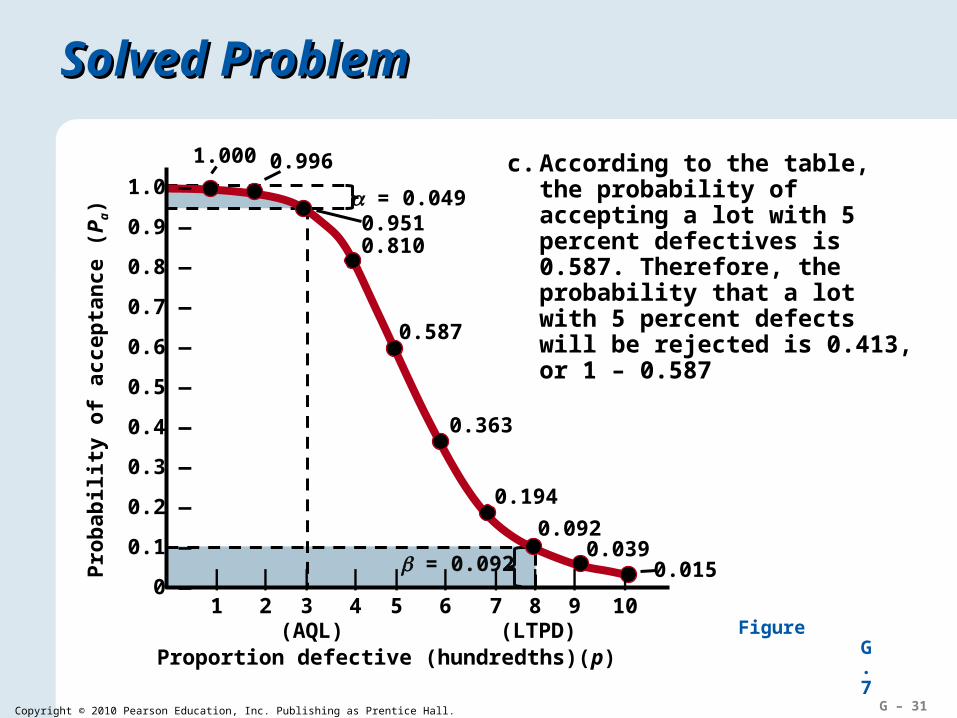
Solved ProblemSolved Problem
c. According to the table, the probability of accepting a lot with 5 percent defectives is 0.587. Therefore, the probability that a lot with 5 percent defects will be rejected is 0.413, or 1 – 0.587
= 0.092
= 0.0491.0 —
0.9 —
0.8 —
0.7 —
0.6 —
0.5 —
0.4 —
0.3 —
0.2 —
0.1 —
0 — | | | | | | | | | |1 2 3 4 5 6 7 8 9 10
Proportion defective (hundredths)(p)
Pro
bab
ility
of
acce
pta
nce
(P
a)
(AQL) (LTPD)
0.996
0.9510.810
0.587
0.363
0.194
0.0920.039
0.015
1.000
Figure G.7

G – 32Copyright © 2010 Pearson Education, Inc. Publishing as Prentice Hall.