fuzzy rule base design using tabu search algorithm for nonlinear system modeling
TRANSCRIPT
ISA Transactions 47 (2008) 32–44www.elsevier.com/locate/isatrans
Fuzzy rule base design using tabu search algorithm for nonlinearsystem modeling
Aytekin Bagis∗
Department of Electrical Electronic Engineering, Erciyes University, 38039 Kayseri, Turkey
Received 15 February 2007; received in revised form 29 August 2007; accepted 4 September 2007Available online 22 October 2007
Abstract
This paper presents an approach to fuzzy rule base design using tabu search algorithm (TSA) for nonlinear system modeling. TSA is used toevolve the structure and the parameter of fuzzy rule base. The use of the TSA, in conjunction with a systematic neighbourhood structure for thedetermination of fuzzy rule base parameters, leads to a significant improvement in the performance of the model. To demonstrate the effectivenessof the presented method, several numerical examples given in the literature are examined. The results obtained by means of the identified fuzzyrule bases are compared with those belonging to other modeling approaches in the literature. The simulation results indicate that the method basedon the use of a TSA performs an important and very effective modeling procedure in fuzzy rule base design in the modeling of the nonlinear orcomplex systems.c© 2007, ISA. Published by Elsevier Ltd. All rights reserved.
Keywords: Fuzzy systems; Fuzzy modeling; Fuzzy rule base design; Nonlinear system modeling; Tabu search
1. Introduction
Modeling is an essential part of control design as it providesa way of formally proving properties of the closed loop system.There are many reasons why a model of a process may berequired. It could, for example, be used to simulate the realprocess or it could be used to design a controller. If a goodmodel of the system can be obtained by using knowledge andobservations, accurate and efficient solutions to engineeringproblems such as system design and simulation, processanalysis, reliability of the measured data, optimization of thesystems can be provided. Conventional system theory relieson crisp mathematical models of systems, such as algebraicand differential equations. However, many real world systemsare inherently nonlinear and cannot be represented by linearmodels used in conventional system identification. For a largenumber of practical problems, the gathering of an acceptabledegree of knowledge needed for physical modeling is a difficult,time consuming and expensive or even impossible task. Expertsystem techniques based on artificial intelligence can provide
∗ Tel.: +90 (0.352) 437 49 37x32255; fax: +90 (0.352) 437 57 84.E-mail address: [email protected].
0019-0578/$ - see front matter c© 2007, ISA. Published by Elsevier Ltd. All rightsdoi:10.1016/j.isatra.2007.09.001
a fast and efficient solution to complex or nonlinear systemmodeling problems. One of the most successful expert systemmethods is fuzzy logic based modeling approach [1].
Rule based fuzzy modeling is a powerful technique forthe modeling of partly known nonlinear systems. In themodeling of complicated and/or ill-defined processes, precisemathematical models may fail to give satisfactory results. Insuch cases, fuzzy models can effectively integrate informationfrom different sources (such as physical laws, empirical models,and experimental measurements) and they may be used toproperly depict the system uncertainty. If fuzzy rule basedmodels can be identified, fuzzy controllers can be obtained fromthe fuzzy models and genuine control engineering issues canbe addressed for fuzzy controllers, namely stability, robustnessetc. [2].
In designing fuzzy models, a major difficulty in theidentification of an optimized fuzzy rule base is encountered.Traditional fuzzy rule design is based upon a human operator’sexperienced knowledge. Not only is this design method timeconsuming since it uses trial and error to find good fuzzyrules and membership functions, it is also not guaranteedto find optimal or near optimal fuzzy rules and membershipfunctions [3,4].
reserved.
A. Bagis / ISA Transactions 47 (2008) 32–44 33
There are many studies on fuzzy modeling in the literature.Takagi and Sugeno proposed a new type of fuzzy modelcalled “Takagi–Sugeno fuzzy model (T–S fuzzy model)” [5].Furthermore, this study proposes a procedure to identify theT–S fuzzy model from input–output data of systems. Sugenoand Yasukawa discussed a general approach to qualitativemodeling based on fuzzy logic [6]. It proposes the use of afuzzy clustering method to identify the structure of a fuzzymodel. Wang and Lee proposed a method based on theback-propagation algorithm to determine significant variableswithout the need of human inspection [7]. A novel fuzzymodeling algorithm was presented by Kim et al. [8]. In thestudy, fuzzy C regression model clustering algorithm and agradient descent algorithm are used. Dynamic versions offuzzy logic systems and their nonsingleton generalizationswere investigated by Mouzouris and Mendel [9]. They useda dynamic learning algorithm to train the system parameters.Wang and Langari presented a fuzzy logic approach tocomplex system modeling that is based on fuzzy discretizationtechnique [10]. A great advantage of the presented approachwas that it could determine the premise structure of a modeloff-line. In [11], a method of Takagi–Sugeno–Kang fuzzymodel generation using numerical data as a starting point wasdescribed by Kukolj.
In addition, many other methods such as neural networksbased methods were suggested and were used to build fuzzymodels [12–15]. Several models for the identification andcontrol of nonlinear dynamic systems were suggested byNarendra and Parthasarathy [13]. These models, which includemultilayer neural networks as well as linear dynamics, can beviewed as generalized neural networks. For the adjustment ofparameters, static and dynamic back-propagation methods areused. Jang described an adaptive network based fuzzy inferencesystem [12]. The presented method employed a hybrid learningprocedure to construct an input–output mapping based onboth human knowledge and stipulated input–output datapairs. By using the architecture of the fuzzy-neural network,simple and effective fuzzy rule based models of complexsystems from input–output data were developed by Lin andCunningham [15]. Babuska and Verbruggen presented anoverview of neuro-fuzzy modeling methods for nonlinearsystem identification [14].
Different optimization algorithms were also used forfuzzy system modeling [16–23]. Hanss presented a specialfuzzy modeling method for developing multivariable fuzzymodels [20]. This fuzzy model identification procedure wascarried out by applying a special clustering method. Kilicet al. proposed a fuzzy system modeling approach based ona probabilistic hill-climbing algorithm as a data analysis andapproximate reasoning tool [19]. Evsukoff et al. used a leastsquares error minimization method for nonlinear fuzzy modelidentification [16]. A genetic based neuro-fuzzy approach formodeling and control of dynamical systems was presented byFarag et al. [23]. The proposed approach combined the merits ofthe fuzzy logic theory, neural networks, and genetic algorithms.Wu and Yu used a genetic algorithm and gradient descent basedapproach to optimize the structure of a Takagi–Sugeno–Kang
model [17]. An evolutionary design method of fuzzy rule basefor nonlinear system modeling and control was presented byKang et al. [22]. Cordon et al. presented an overview of therepresentative methods in genetic fuzzy systems proposed inthe literature [21].
This paper presents an approach to fuzzy rule base designusing a tabu search algorithm (TSA) for nonlinear systemmodeling. TSA is used to evolve the structure and theparameters of fuzzy rule base. To check the effectiveness of thepresented approach, several numerical examples given in theliterature are examined. The results obtained by means of theidentified fuzzy rule bases are compared with those belongingto other modeling approaches in the literature. The remainderof the paper is organized as follows. In Section 2, a brief reviewof the TSA is introduced. Structure of the identified fuzzy rulebase and design method is developed in Section 3. Simulationresults and some conclusions are given in Sections 4 and 5,respectively.
2. Tabu search algorithm (TSA)
TSA was proposed by Glover as an intelligent optimizationtechnique to overcome local optimality in solution processes forhard combinatorial optimization problems [24]. This algorithmconsists of the systematic prohibition of some solutions toprevent cycling and to avoid the risk of trapping at a localoptimum. New solutions are searched in the neighbourhood ofthe current one. In TSA, there are several important concepts:
Neighbourhood: To improve the quality of the solutions visited,the search moves from one solution to another using aneighbourhood structure. The neighbourhood of a solution isthe set of all formations that can be arrived at by a move.The move is a process that transforms the current solution toits neighbouring solution. If, after making a move, a solutionis found which is better than all solutions found in priormoves than the new solution is saved as the new best solution.This neighbourhood procedure is applied to the only one bestsolution of each generation. Considering a chromosome with nbits, the number of the neighbour solutions is n, as depicted inFig. 1. To obtain the neighbour solutions for the best solution,encoding and decoding operations are applied. In this work,using different bit sizes for each of the parameters we have triedto achieve a good balance between the algorithm performanceand the computational cost, and we finally adopt a bit sizeof 8. Therefore, total number of bits required for defining afuzzy rule base parameter set is [rule number × parameternumber × bit number]. According to simulation results, this bitsize is suitable for the main process in the algorithm describedin this paper.
Tabu list: One of the main ideas of TSA is the use of aflexible memory (tabu list). The objective of the tabu list is toexclude moves which would bring the algorithm back to whereit was at some previous iteration and keep it trapped in a localminimum. To avoid performing a move returning to a recentlyvisited region, the reverses of last moves are forbidden. In otherwords, these moves are considered as “tabu” and are recordedin the tabu list. The tabu list stores all tabu moves that are

34 A. Bagis / ISA Transactions 47 (2008) 32–44
Fig. 1. Neighbourhood structure for a solution.
Table 1The values of the control parameters for TSA
Tabu search algorithm
Recency factor (r ) 0.2Frequency factor ( f ) 2.0Generation number 2000Tabu conditions (1) Recency (k) > (r × M),
(2) Frequency (k) < ( f × avgfreq)
Number of variables for a rule 9, for system with 2 inputs and 1 output13, for system with 3 inputs and 1 output
Number of neighbourhood pervariable
8
Tabu list size Rule number × number of the variables
not permitted to be applied to the present solution. This list isinitialized empty, constructed in consecutive iterations of thesearch and updated circularly in later iterations.
Tabu conditions: The number of the possible moves isdetermined by the tabu list. If a solution produced by a movethat is not on the tabu list is better than all solutions found inprior iterations, then this solution is saved as the best solution.At each of the iterations in the optimization process, candidatesolutions are checked with respect to “tabu conditions”, andhence, the next solution is determined depending on evaluationvalues and tabu conditions. The re-generation of a solutionpreviously obtained is avoided by using the tabu conditions(or restrictions) on the possible moves. The tabu conditionsare usually based on two important factors: frequency memoryand recency memory. Frequency memory keeps the knowledgeof how often the same solutions have been made in the past.Recency memory prevents cycles of length less than or equal toa predetermined number of iterations. The tabu conditions usedin this work are as the following: If the element k of a solutionvector does not satisfy the conditions (i) recency (k) > r.M ,(ii) frequency (k) < f.avgfreq, then it is accepted as tabu andnot used to create a neighbour. Here, r and f are recency andfrequency factors, M is the number of elements in the solutionvector, and avgfreq is the average frequency value. In this work,after some experimentation, the algorithm parameters r and fhave been set to the values of 0.2 and 2.0, respectively. Thecontrol parameter values for the TS algorithm are given inTable 1. For all of the simulations, the iteration or generationnumber is taken as 2000. The number of bits per variable is 8.Thus, if a rule has the n parameters, the total number of bits inthe string describing each member of the solutions is (n × 8).
Fig. 2. System modeling scheme.
Aspiration criterion: TS has another important element calledaspiration mechanism. If a move on the tabu list leads to asolution with a value strictly better than the best obtained sofar, it is possible to allow this move to get out of the tabu list.This property is used to avoid removing very good moves fromconsideration and plays an essential role in the search process.In this work, if all available moves are classified as tabu, then aleast tabu move is selected for a new solution. The least tabumove means that this solution is changed less recently andfrequently among them but it is still classified as tabu. In thiswork, maximum number of iterations reached is selected as thestopping criterion of the search process.
The basic procedure of TSA to be utilized in this paper isdescribed as follows:
Initial solution;While predetermined stopping criteria not satisfied;{
Create a set of neighbour solutions;Evaluate the neighbour solutions;Choose the best admissible solution;Test the tabu conditions;Perform the aspiration test;Update tabu list;}
This procedure is repeated until a satisfactory solution isobtained or predetermined number of generations is elapsed.For all of the modeling examples, the number of the generationwas selected as 2000.
3. Structure of the identified fuzzy rule base
Fig. 2 shows the system modeling scheme. In this figure,yp(t + 1) is the output of the system to be modeled, andym(t + 1) is the output of the fuzzy model optimized by theTSA. Input of the TSA is the error value, and it is calculatedby {error = yp(t + 1) − ym(t + 1)}. The major objective ofthe algorithm is to determine the most appropriate fuzzy modelparameters and to reduce the error factor.
In fuzzy models, structure selection involves the followingchoices:
(a) input and output variables(b) structure of the rules

A. Bagis / ISA Transactions 47 (2008) 32–44 35
Fig. 3. (a) Parameter matrix representing the membership functions, (b) Fuzzy rule base represented by parameter matrices, (c) The rule base coding.
(c) number and type of membership functions for each variable(d) type of the inference mechanism, connective operators,
defuzzification method.
After the structure is fixed, the performance of a fuzzymodel can be fine-tuned by adjusting its parameters. Tunableparameters of linguistic models are the antecedent parametersand consequent membership functions and the rules. Rulesin the fuzzy rule base are described by the membershipfunctions. Fuzzy membership functions can have differentshapes depending on the designer’s preference or experience.In general, fuzzy engineers have found that triangular andtrapezoidal shapes help capture the modeller’s sense offuzzy numbers and simplify computation. In this study, inputvariables are characterized by triangular membership functions,and the output variables are characterized by fuzzy singletons.A rule in the rule base has a general form expressed by
Ri : If x1 is Ai1(x1) and x2 is Ai
2(x2) then y is Bi (1)
where Ri is the i th rule, xj is the input variable, and y is theoutput variable. Ai
j(xj) is the fuzzy linguistic value defined as
in Eq. (2) and Bi takes the role of fuzzy singleton, i.e., realnumber.
Aij = max(min[(xj − a)/(b − a), (c − xj)/(c − b)], 0). (2)
In Eq. (2); a, b, and c are the main parameters of a triangularmembership function. These parameters represent the locationsof starting point, peak point, and the ending point for a triangleshaped membership function, respectively.
Deciding the number of fuzzy rules is a very criticalissue since it plays key roles in the fuzzy modeling of thesystems. Except for some propositions, unfortunately, there isno systematic and efficient procedure for choosing the most
appropriate rule number. A reasonable number of fuzzy ruleswithout losing too much information about the system tobe modeled must be carefully obtained. In this work, usingdifferent rule sizes we have tried to achieve a good balancebetween the model performance and rule complexity.
Another important element in combining a TSA and afuzzy model is the encoding method used to represent afuzzy rule base as a probable solution element on which theTSA operates. Selecting an appropriate encoding procedureis a critical factor that affects the efficiency of the TSA andthe final solution. The membership functions of the inputvariables are characterized by three numerical values. Onthe other hand, the output variables are defined by singletonnumerical values. These numerical values represent the positionof the membership function on the universe of discourse. Theparameter matrix defining the membership functions and fuzzyrule base represented by the parameter matrices is formulatedin Fig. 3. The parameter matrix that contains the parametersfor defining the membership functions within the fuzzy rulebase will be of one-dimensional matrix form. For each rulein the fuzzy rule base, the adjustment parameters used in thereasoning procedure are also involved in this parameter matrix.In Fig. 3, these parameters are stated by di for each inputvariable. Thus, the size of matrix is determined by {the numberof rules × [(the number of input variables × 3) + (the numberof output variables × 1) + (the number of input variables)]}.This value of the matrix is also equal to the size of the tabulist. For a fuzzy model with two inputs and one output, eachfuzzy rule is represented by nine parameters. The rule structurecoding is organized as shown in Fig. 3(c). For example, if themodeling system has two inputs and one output, 144 bits areused to represent a probable solution with two rules optimizedby the algorithm (Fig. 3(c)). Initializing the solution is based

36 A. Bagis / ISA Transactions 47 (2008) 32–44
Table 2Optimized parameter matrix for fuzzy rule base
Rules Input 1, u(t − 4) Input 2, y(t − 1) Output, y(t) Adjustment parametersai1 ai2 ai3 bi1 bi2 bi3 ci di1 di2
Normalized parameters(1) 0.1579 0.1720 0.4845 0.1485 0.3595 1.0196 0.7658 0.4863 0.2813(2) 0.0552 0.3294 2.5020 0.0000 0.2667 0.8046 0.0156 0.1489 0.5020(3) 0.0000 0.1569 0.8908 0.3476 1.8823 2.7922 0.9412 0.4706 1.1214(4) 0.5640 0.7529 1.2549 0.2813 0.4072 0.8314 0.2500 0.2510 0.0784
Denormalized parameters(1) −2.0526 −1.9680 −0.0930 46.6730 50.4710 62.3528 57.7844 0.4863 0.2813(2) −2.6688 −1.0236 12.0120 44.0000 48.8006 58.4828 44.2808 0.1489 0.5020(3) −3.0000 −2.0586 2.3448 50.2568 77.8814 94.2596 60.9416 0.4706 1.1214(4) 0.3840 1.5174 4.5294 49.0634 51.3296 58.9652 48.5000 0.2510 0.0784
on the randomly generated values from the given searchingintervals.
In this study, the following reasoning procedures areconsidered:
(a) Given input data x1 and x2, calculate the degree of thefulfillment ωi in the premise for the i th rule as in
ωi = Ai1(x1k).di1 + Ai
2(x2k).di2,
k = input data number. (3)
(b) Calculate the inferred value yi by taking the weightedaverage of Bi with respect to ωi as in
yi =
r∑i=1
ωi.Bi
r∑i=1
ωi
(4)
where r is the number of fuzzy rules.
To evaluate the performance of a fuzzy model, there are twoimportant performance indices in the literature. These are themean squared error (MSE) and a performance parameter statedas PI. In the MSE, the error is the difference between the actualoutput and the estimated output by the fuzzy model. The MSEand PI are calculated from N data point as
MSE =1N
N∑k=1
(Odk − Ok)
2 (5a)
PI =
√N∑
k=1(Od
k − Ok)2
N∑k=1
∣∣Odk
∣∣ (5b)
where Odk , k = 1, . . . , N are the actual or desired output values
and Ok , k = 1, . . . , N are the outputs from the model.These performance indices provide a means for evaluating
the performance of a fuzzy model with the selected fuzzyrule base in the process of evolution, so that an optimizedmodel would be developed by the best individual. During theevolution, the quality of the best solution at each generation iscalculated by Eq. (5a) or (5b).
4. Simulation results
Five numerical examples are provided in this section toillustrate the performance of the presented approach. All theseexamples have their origin in the existing literature. Thedatasets used in the first and third examples are derived frompractical processes; while the dataset used in the second andfourth examples is generated from the simulation of analyticalmodels. In the first example, the fuzzy modeling of a dynamicalprocess using a famous example of the system identificationgiven by Box and Jenkins [25] is discussed. The third exampleis used to show how to build a model of a human operator’scontrol action in a chemical plant. The structure of the humanoperation is shown in Sugeno and Yasukawa [6]. Furthermore,input–output data for human operation at the chemical processare also listed in [17]. In the fifth example, modeling of a realreservoir system is considered [3,4]. And, the datasets used inthis example are real flood hydrograph data of the dynamicalsystem.
(a) Box and Jenkins’ gas furnace: The fuzzy model of adynamic process using a well-known example of the systemidentification given by Box and Jenkins is considered [6,22,25].The process is a gas furnace with a single input u(t) and a singleoutput y(t): gas flow rate and CO2 concentration, respectively.The dataset consists of N = 296 pairs of input–outputmeasurements. The inputs to the fuzzy model were selected asu(t−4), y(t−1), respectively. The model output is y(t). For thevariables of u(t −4), y(t −1), and y(t), normalization intervalswere selected as [−3, 3], [44, 62], and [44, 62], respectively.Parameters of the fuzzy model were searched into the intervalof [0, 4]. During the evolution, the modeling error of the bestindividual at each generation was calculated by Eq. (5a). Theoptimized fuzzy model for a gas furnace and the comparison ofmodel outputs and the original output data are shown in Figs. 4and 5, and the modeling error is 0.1483. The number of rulesin the fuzzy model is only four. Normalized and denormalizedparameter matrices of the fuzzy model are also given in Table 2.In Table 3, our fuzzy model is compared with other modelsidentified from the same data.
(b) Modeling of a static nonlinear function: In this subsection,double input and single output static function was chosen as

A. Bagis / ISA Transactions 47 (2008) 32–44 37
Fig. 4. Optimized fuzzy rule base for gas furnace.
Fig. 5. Comparison of model outputs and original output data for the gasfurnace.
a target system. The function was taken from Narendra andParthasarathy [13] and represented as
y = (1 + x−21 + x−1.5
2 )2, 1 ≤ x1, x2 ≤ 5 (6)
from which 50 data was obtained. From this system equation,50 input–output data are obtained. In this instance, two randominputs x1 and x2 were inserted to test input identification.Normalization intervals for input–output parameters x1, x2, ywere selected as [0, 6], [0, 6], [0, 10], respectively. Modelparameters were searched in the interval of [0, 4]. During theevolution, the modeling error at each generation was calculatedby Eq. (5a). The optimized fuzzy model for nonlinear systemand the comparison of model outputs and the original outputdata are shown in Figs. 6 and 7, respectively, and the modelingerror is 0.0019. The rule number of the fuzzy model is
Table 3Comparison of our model with other models
Method Rule number MSE
Box and Jenkins (1970) [25] – 0.202Tong (1978) [26] 19 0.469Pedrycz (1984) [27] 81 0.320Takagi and Sugeno (1985) [5] 6 0.190Xu and Lu (1987) [28] 25 0.328Sugeno and Tanaka (1991) [29] 2 0.068Sugeno and Tanaka (1991) [29] 2 0.359Wang and Langari (1996) [10] 5 0.158Nakoula et al. (1997) [30] 90 0.175Kim et al. (1997) [8] 2 0.055Farag et al. (1998) [23] 37 0.111Kang et al. (2000) [22] 5 0.161Evsukoff et al. (2002) [16] 36 0.153Evsukoff et al. (2002) [16] 90 0.090Our model 4 0.148
five. Normalized and denormalized parameter matrices of thefuzzy model are given in Table 4. Performance indices of thepresented method and the other methods in the literature aregiven in Table 5. To test the validity of the derived model,the later 20 data that are not used in the model derivation areconsidered by the model, where MSE calculated by (5a) is0.0043 (Fig. 7(b)).
(c) Human operation at a chemical plant: This exampledeals with the modeling of human operator control in achemical plant. The plant is for producing a polymer by thepolymerization of monomers. Since the start-up of the plant isvery complicated, a human operator is used to manually operatethe system in this circumstance. The structure of the humanoperation is given by Sugeno and Yasukawa [6]. Five inputcandidates, u1: the monomer concentration, u2: the change ofmonomer concentration, u3: the monomer flow rate, u4 and u5:

38 A. Bagis / ISA Transactions 47 (2008) 32–44
Fig. 6. Optimized fuzzy rule base for a static nonlinear function.
Fig. 7. (a) Comparison of model outputs and original output data for example (b). (b) Test outputs and model outputs for example (b).
the local temperature inside the plant are available, to whichthe human operator may refer. The output y is the set point formonomer flow rate. There are 70 data points for each of theabove six variables (five inputs, and one output).
There are different fuzzy models available for modeling thisplant. In [6], a six rule qualitative fuzzy model was given byidentifying u1, u2, and u3 as input variables. In [10], u1, u2,and u3 were selected as the input variables, and six clustersfrom the given data were taken to give six rules and threepremise variables of the Takagi–Sugeno–Kang model. In [15],a fuzzy-neural system was used for modeling the plant. Theperformance measurement was not stated in [6] and [10].
In our approach, the input variables u1 and u3 were selectedto build the fuzzy model. Normalization intervals for allvariables (u1, u3, y) were selected as [4, 7], [0, 8000], and[0, 8000], respectively. Model parameters were searched in thesolution area of [0, 2]. During the evolution, the modeling errorat each generation was calculated by Eq. (5b). Optimized modelparameters and optimum rule base are given in Table 6 andFig. 8, respectively. Optimum rule base has only three rules.The comparison of model outputs and the original output dataare shown in Fig. 9. In Table 7, our fuzzy model is comparedwith the other models in the literature.

A. Bagis / ISA Transactions 47 (2008) 32–44 39
Table 4Optimized parameter matrix for fuzzy rule base
Rules Input 1, x1 Input 2, x2 Output, y Adjustment parametersai1 ai2 ai3 bi1 bi2 bi3 ci di1 di2
Normalized parameters(1) 0.5348 0.7867 0.7887 0.3438 0.7735 0.8282 0.1730 0.0625 1.4922(2) 0.2285 0.2286 0.5411 0.0000 0.0728 0.3282 1.0000 0.1279 0.2500(3) 0.1661 0.2247 3.1662 0.1641 0.3141 0.6661 0.2328 0.2731 1.0490(4) 0.1661 0.2516 0.2657 0.0938 0.5781 1.9137 0.0313 0.3516 0.5742(5) 0.0938 0.0956 0.2657 0.2130 0.3439 0.3594 0.9705 1.7887 0.0509
Denormalized parameters(1) 3.2088 4.7202 4.7322 2.0628 4.6410 4.9692 1.7300 0.0625 1.4922(2) 1.3710 1.3716 3.2466 0.0000 0.4368 1.9692 10.000 0.1279 0.2500(3) 0.9966 1.3482 18.9972 0.9846 1.8846 3.9966 2.3280 0.2731 1.0490(4) 0.9966 1.5096 1.5942 0.5628 3.4686 11.4822 0.3130 0.3516 0.5742(5) 0.5628 0.5736 1.5942 1.2780 2.0634 2.1564 9.7050 1.7887 0.0509
Fig. 8. Optimized fuzzy rule base for human operation at a chemical plant.
Table 5Comparison of different models for example (b)
Method Rule number MSE
Sugeno and Yasukawa (1993) [6] 6 0.0790Lin and Cunningham (1995) [15] 3 0.0035Kim et al. (1997) [8] 3 0.0197Our model 5 0.0019
(d) Nonlinear differential equation: This example is takenfrom Narendra and Parthasarathy [13] in which the plant tobe identified is given by the second-order highly nonlineardifference equation
y(k) =y(k − 1).y(k − 2).(y(k − 1) + 2.5)
1 + y2(k − 1) + y2(k − 2)+ u(k). (7)
Training data of 500 points are generated from the plantmodel, assuming a random input signal u(k) uniformlydistributed in the interval [−2, 2]. This unpredictable input“u(k)” is randomly generated and is inserted into the system.The first 500 data points are produced from (7) for modelidentification. To demonstrate the performance of the fuzzy
Fig. 9. Comparison of model outputs and original output data for the chemicalplant.
model, a different type sinusoidal input data u(k) is insertedinto the system y(k) (Fig. 10).
The model has three inputs u(k), y(k − 1), and y(k − 2),and a single output y(k). Normalization intervals for the inputs
40 A. Bagis / ISA Transactions 47 (2008) 32–44
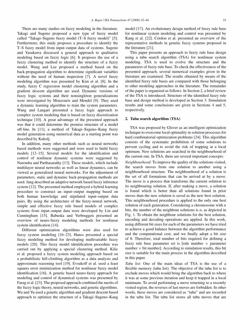
Table 6Optimized parameter matrix for fuzzy rule base
Rules Input 1, u1 Input 2, u3 Output, y Adjustment parametersai1 ai2 ai3 bi1 bi2 bi3 ci di1 di2
Normalized parameters(1) 0.0000 0.3130 1.1006 0.5938 1.4525 1.4642 0.8827 0.2544 1.4486(2) 0.1719 0.4840 0.7141 0.4527 0.4844 0.8908 0.4172 0.0774 0.3157(3) 0.2537 0.3387 0.6829 0.0430 0.0489 0.5266 0.0110 0.0351 0.8387
Denormalized parameters(1) 4.0000 4.9390 7.3018 4750.40 11 620.00 11 713.60 7061.60 0.2544 1.4486(2) 4.5157 5.4520 6.1423 3621.60 3 875.20 7 126.40 3337.60 0.0774 0.3157(3) 4.7611 5.0161 6.0487 344.00 391.20 4 212.80 88.00 0.0351 0.8387
Table 7Comparison of different models for human operation at a chemical plant
Method Modelinputs
Rulenumber
PI
Sugeno and Yasukawa(1993) [6]
u1, u2, u3 6 Not stated
Lin and Cunningham(1995) [15]
u1, u2, u3 7 0.002245
Wu and Yu (2000) [17] u3, u4 4 0.002000Our model u1, u3 3 0.001700
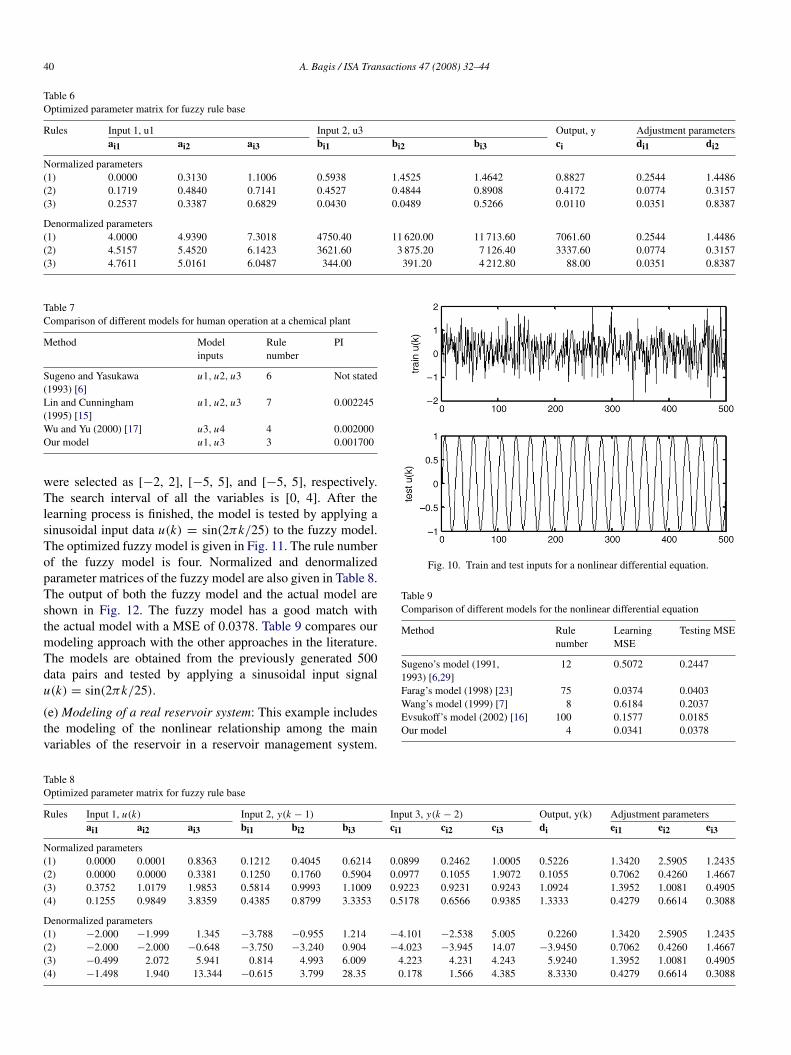
were selected as [−2, 2], [−5, 5], and [−5, 5], respectively.The search interval of all the variables is [0, 4]. After thelearning process is finished, the model is tested by applying asinusoidal input data u(k) = sin(2πk/25) to the fuzzy model.The optimized fuzzy model is given in Fig. 11. The rule numberof the fuzzy model is four. Normalized and denormalizedparameter matrices of the fuzzy model are also given in Table 8.The output of both the fuzzy model and the actual model areshown in Fig. 12. The fuzzy model has a good match withthe actual model with a MSE of 0.0378. Table 9 compares ourmodeling approach with the other approaches in the literature.The models are obtained from the previously generated 500data pairs and tested by applying a sinusoidal input signalu(k) = sin(2πk/25).
(e) Modeling of a real reservoir system: This example includesthe modeling of the nonlinear relationship among the mainvariables of the reservoir in a reservoir management system.
Table 8Optimized parameter matrix for fuzzy rule base
Rules Input 1, u(k) Input 2, y(k − 1) Input 3, y(k − 2) Output, y(k) Adjustment parametersai1 ai2 ai3 bi1 bi2 bi3 ci1 ci2 ci3 di ei1 ei2 ei3
Normalized parameters(1) 0.0000 0.0001 0.8363 0.1212 0.4045 0.6214 0.0899 0.2462 1.0005 0.5226 1.3420 2.5905 1.2435(2) 0.0000 0.0000 0.3381 0.1250 0.1760 0.5904 0.0977 0.1055 1.9072 0.1055 0.7062 0.4260 1.4667(3) 0.3752 1.0179 1.9853 0.5814 0.9993 1.1009 0.9223 0.9231 0.9243 1.0924 1.3952 1.0081 0.4905(4) 0.1255 0.9849 3.8359 0.4385 0.8799 3.3353 0.5178 0.6566 0.9385 1.3333 0.4279 0.6614 0.3088
Denormalized parameters(1) −2.000 −1.999 1.345 −3.788 −0.955 1.214 −4.101 −2.538 5.005 0.2260 1.3420 2.5905 1.2435(2) −2.000 −2.000 −0.648 −3.750 −3.240 0.904 −4.023 −3.945 14.07 −3.9450 0.7062 0.4260 1.4667(3) −0.499 2.072 5.941 0.814 4.993 6.009 4.223 4.231 4.243 5.9240 1.3952 1.0081 0.4905(4) −1.498 1.940 13.344 −0.615 3.799 28.35 0.178 1.566 4.385 8.3330 0.4279 0.6614 0.3088
Fig. 10. Train and test inputs for a nonlinear differential equation.
Table 9Comparison of different models for the nonlinear differential equation
Method Rulenumber
LearningMSE
Testing MSE
Sugeno’s model (1991,1993) [6,29]
12 0.5072 0.2447
Farag’s model (1998) [23] 75 0.0374 0.0403Wang’s model (1999) [7] 8 0.6184 0.2037Evsukoff’s model (2002) [16] 100 0.1577 0.0185Our model 4 0.0341 0.0378
A. Bagis / ISA Transactions 47 (2008) 32–44 41
Fig. 11. Optimized fuzzy rule base for the nonlinear differential equation.
Fig. 12. Comparison of model outputs and original output data for thenonlinear differential equation.
Reservoir management system is a control system that managesa spillway gate in a dam to increase or decrease the amountof discharge water [3,4,31]. Reservoir management is acomplex, nonlinear, nonstationary control process because: (a)The hydrological conditions have a nonlinear behavior, (b)Determination of the inflow hydrograph can be extremelydifficult, (c) Construction of a precise model of this process isvery difficult, (d) Owing to human factor, accurate and efficientcontrol of the process is quite difficult.
The main variables of a reservoir are reservoir lake level (H ,m), spillway gate opening (d , m) and released water amount(Q, m3/s) [3,4,31]. The fuzzy model is used to model thenonlinear relationship among these variables. Lake level (H )and spillway gate opening (d) are the inputs of the model. Theoutput variable of the fuzzy model is the released water amount(Q). In this work, the reservoir system of Adana Catalan Damin Turkey is considered, and the real flood hydrograph data for
Catalan Dam are used [31]. To generate comparable results tothose already published; the 548 real data points were usedto generate a model using the TSA based method. At the endof the training process, the resultant model was applied to thevalidation dataset, which was the dataset of 25 unseen data. Allof the above information is obtained from the file containing thefinal project details of Catalan Dam [31].
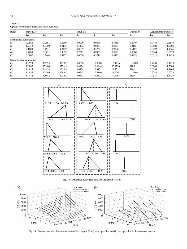
Normalization intervals for input–output parameters H, d, Qwere selected as [117, 131], [0, 12], [0, 10 000], respectively.Model parameters were searched in the interval of [0, 10]. Op-timized model parameters and optimum rule base are given inTable 10 and Fig. 13, respectively. The PI was calculated forthe model predictions of the validation data and the results havebeen given in Table 11. The optimum rule base has only fiverules. The comparison of model outputs and the original outputdata is shown in Fig. 14 as three dimensions. In Fig. 15, processoutputs for train and test data are given as two dimensions. Theresults show that the fuzzy rule structure optimized by the TSAcan yield a better model than the model which has the struc-ture of a neural network, improving the validation data modelprediction PI.
Because it did not seem to be the most commonly usedparameter in the literature to be considered, the time parameterwas not selected as a comparison parameter. The values of thecomputation time were not stated mostly in the literature to becompared. However, to indicate the computational performanceof the TSA, the computation time per evaluation of thealgorithm for each problem is given in Table 12. In thesimulations, Matlab programming package and Pentium IV3600 MHz computer were used.
It is clear from the figures that fuzzy modeling based TSAis a powerful tool for modeling of nonlinear systems. Theapproach is easy to use and there is no difficulty in writing itsalgorithm based modeling procedure.
42 A. Bagis / ISA Transactions 47 (2008) 32–44
Table 10Optimized parameter matrix for fuzzy rule base
Rules Input 1, H Input 2, d Output, Q Adjustment parametersai1 ai2 ai3 bi1 bi2 bi3 ci di1 di2
Normalized parameters(1) 0.0566 0.0661 0.6299 0.0000 0.0000 0.5368 0.0049 1.7488 2.4610(2) 1.3333 4.0000 4.3175 0.5402 0.8887 2.8233 0.8105 0.0000 1.2308(3) 0.1604 0.1631 1.3449 0.0059 0.5761 0.9376 0.5102 0.0293 1.1965(4) 0.4688 0.6421 0.9029 0.7512 0.8905 0.9922 0.0000 0.2344 0.0778(5) 0.0802 0.2444 0.4727 0.0056 0.3711 0.8422 0.4859 0.0510 1.1429
Denormalized parameters(1) 117.79 117.93 125.82 0.0000 0.0000 6.4416 49.00 1.7488 2.4610(2) 135.67 173.00 177.45 6.4824 10.6644 33.8796 8105 0.0000 1.2308(3) 119.25 119.28 135.83 0.0708 6.9132 11.2512 5102 0.0293 1.1965(4) 123.56 125.99 129.64 9.0144 10.6860 11.9064 0.00 0.2344 0.0778(5) 118.12 120.42 123.62 0.0672 4.4532 10.1064 4859 0.0510 1.1429
Fig. 13. Optimized fuzzy rule base for a reservoir system.
Fig. 14. Comparison with three dimensions of the outputs for (a) train operation and (b) test operation in the reservoir system.

A. Bagis / ISA Transactions 47 (2008) 32–44 43
Fig. 15. Comparison with two dimensions of the outputs for (a) train operation and (b) test operation in the reservoir system.
Table 11Comparison of different models for a nonlinear reservoir system
Method Model inputs PI (train) PI (test)
Neural model [31] H, d 0.00170 0.0056Our model H, d 0.00158 0.0065
When the model performance and rule size are considered,the resulting outcome is quite exciting. It is clear from the tablesthat a striking reduction in the value of the performance index(MSE or PI) is obtained without the need of a large number ofrules. The low rule size is a significant advantage of the model.
The studies in the literature show that TSA is an effectiveoptimization method in the designing of fuzzy systems [3, 4].By using the control factors such as the initial solution, type ofmove, size of neighbourhood, tabu list size, aspiration criterionand stopping criterion, the performance of the algorithm can besignificantly improved. And, system models with high qualitycan be obtained.
Three important conclusions can be made from the details ofthe numerical results:
First, the requirement for using the large number of rules issuccessfully removed by employing the TSA. Tabu algorithmenables us to obtain better results when the number ofmembership functions and rules is as small as possible to solvethe problem at hand, a realistic case from an industrial point ofview. With tabu search, it is indeed possible to optimally tunethe structure of the fuzzy model.
Second, even though the presented approach does not showthe best performance for all of the problem types considered, itobviously exhibits a competitive performance for the modelingof the nonlinear or complex systems. It has the ability ofgetting out of local minima and finding global optimal solutions
for multimodal problems in a reasonable time although thetraditional optimization algorithms fail to produce globaloptimal solution for such problems. Thus, it is verified thatthe presented method is capable of defining the nonlinearitiesor uncertainties of the system conditions without requiringany expert knowledge or experience about the system to beconsidered.
Third, the numerical results show that the modelingapproach based on the TSA has high accuracy (low error)and good generalization ability. Moreover, it can start tolearn a process from a very low number of initial datasamples and improve the performance of the initial model.Therefore, it can be used effectively for various engineeringproblems in different areas with the nonlinear behaviors. And,accurate, fast, and reliable fuzzy models can be developed frommeasured/simulated data.
When the process is highly nonlinear, time varying, or whenit depends on a lot of parameters, the cost for getting an accuratemodel is often estimated as being too high. In this case, fuzzymodeling approach based on the use of TSA can be viewed asa useful alternative method.
5. Conclusion
In this paper, an efficient approach to fuzzy rule basedesign using the tabu search algorithm for nonlinear systemmodeling is presented. To demonstrate the effectiveness of thepresented approach, several numerical examples given in theliterature are examined. Simulation results show that the fuzzymodeling approach presented here is a powerful tool for themodeling of nonlinear systems. As compared with the othermodeling methods, the described approach has the advantagesof simplicity, flexibility, and high accuracy. The method is
Table 12Computational performance of the TSA for different problems
Problem Datanumber
Rulenumber
Parameter numberper rule
Total parameternumber
Neighbourhoodnumber
Computation time per iteration (s)
Box–Jenkins 296 4 9 36 288 9.18 (for 288 evaluation)Static nonlinear function 50 5 9 45 360 2.37 (for 360 evaluation)Chemical plant 70 3 9 27 216 1.27 (for 216 evaluation)Nonlinear differentialequation
500 4 13 52 416 31.27 (for 416 evaluation)
Reservoir operation 548 5 9 45 360 24.13 (for 360 evaluation)

44 A. Bagis / ISA Transactions 47 (2008) 32–44
easy to use and there is no difficulty in writing its automaticmodeling procedure. Especially, when the model performanceand rule size are considered, the method based on the use of atabu search algorithm performs an important and very effectivemodeling procedure to fuzzy rule base design in the modelingof nonlinear or complex systems.
Acknowledgements
The author is grateful to the reviewers, and Prof. DervisKaraboga at Erciyes University in Turkey for their valuablecomments and suggestions.
References
[1] Babuska R. Fuzzy modeling for control. Kluwer Academic Pub.; 1998.[2] Nguyen HT, Sugeno M. Fuzzy systems: Modeling and control. Kluwer
Academic Pub.; 1998.[3] Bagis A. Fuzzy and PD controller based intelligent control of spillway
gates of dams. J Intell Fuzzy Syst 2003;14(1):25–36.[4] Bagis A. Determining fuzzy membership functions with tabu search—An
application to control. Fuzzy Sets and Systems 2003;139:209–25.[5] Takagi T, Sugeno M. Fuzzy identification of systems and its applications
to modeling and control. IEEE Trans Syst Man Cybern 1985;15:116–32.[6] Sugeno M, Yasukawa T. A fuzzy logic based approach to qualitative
modeling. IEEE Trans Fuzzy Syst 1993;1(1):7–31.[7] Wang S, Lee C. Fuzzy system modeling using linear distance rules. Fuzzy
Sets and Systems 1999;108:179–91.[8] Kim E, Park M, Ji S, Park M. A new approach to fuzzy modeling. IEEE
Trans Fuzzy Syst 1997;5(3):328–37.[9] Mouzouris GC, Mendel JM. Dynamic non-singleton fuzzy logic systems
for nonlinear modeling. IEEE Trans Fuzzy Syst 1997;5(2):199–208.[10] Wang L, Langari R. Complex systems modeling via fuzzy logic. IEEE
Trans Syst Man Cybern-Part B: Cybern 1996;26(1):100–6.[11] Kukolj D. Design of adaptive Takagi–Sugeno–Kang fuzzy models. Appl
Soft Comput 2002;2:89–103.[12] Jang JR. ANFIS: adaptive network based fuzzy inference system. IEEE
Trans Syst Man Cybern 1993;23(3):665–85.[13] Narendra KS, Parthasarathy K. Identification and control of dynamical
systems using neural networks. IEEE Trans Neural Netw 1990;1(1):4–27.[14] Babuska R, Verbruggen H. Neuro-fuzzy methods for nonlinear system
identification. Ann Rev Control 2003;27:73–85.
[15] Lin Y, Cunningham GA. A new approach to fuzzy-neural systemmodeling. IEEE Trans Fuzzy Syst 1995;3(2):190–8.
[16] Evsukoff A, Branco ACS, Galichet S. Structure identification andparameter optimization for non-linear fuzzy modeling. Fuzzy Sets andSystems 2002;132:173–88.
[17] Wu B, Yu X. Fuzzy modeling and identification with genetic algorithmbased learning. Fuzzy Sets and Systems 2000;113:351–65.
[18] Pham DT, Castellani M. Evolutionary learning of fuzzy models. Eng ApplArtif Intell 2006;19:583–92.
[19] Kilic K, Sproule BA, Turksen IB, Naranjo CA. A fuzzy system modelingalgorithm for data analysis and approximate reasoning. Robot Auton Syst2004;49(3–4):173–80.
[20] Hanss M. Identification of enhanced fuzzy models with specialmembership functions and fuzzy rule bases. Eng Appl Artif Intell 1999;12:309–19.
[21] Cordon O, Herrera F, Hoffman F, Magdalena L. Genetic fuzzy systems:Evolutionary tuning and learning of fuzzy knowledge bases. Singapore,New Jersey, London, Hong Kong: World Scientific; 2001.
[22] Kang S, Woo C, Hwang H, Woo KB. Evolutionary design of fuzzy rulebase for nonlinear system modeling and control. IEEE Trans Fuzzy Syst2000;8(1):37–45.
[23] Farag WA, Quintana VH, Torres GL. A genetic based neuro-fuzzyapproach for modeling and control of dynamical systems. IEEE TransNeural Netw 1998;9(5):756–67.
[24] Pham DT, Karaboga D. Intelligent optimisation techniques: Geneticalgorithms, tabu search, simulated annealing and neural networks.Springer-Verlag; 2000.
[25] Box GEP, Jenkins GM. Time series analysis, forecasting, and control. SanFrancisco (CA): Holden Day; 1970.
[26] Tong RM. Synthesis of fuzzy models for industrial processes-some recentresults. Int J General Syst 1978;(4):143–62.
[27] Pedrycz W. An identification algorithm in fuzzy relational systems. FuzzySets and Systems 1984;(13):153–67.
[28] Xu CW, Lu YZ. Fuzzy model identification and self-learning for dynamicsystems. IEEE Trans Syst Man Cybern 1987;(17):683–9.
[29] Sugeno M, Tanaka K. Successive identification of a fuzzy model and itsapplication to prediction of a complex system. Fuzzy Sets and Systems1991;(42):315–34.
[30] Nakoula Y, Galichet S, Foulloy L. A learning method for structure andparameter identification of fuzzy linguistic models. In: Hellendoorn H,Driankov D, editors. Selected approaches to fuzzy model identification.Berlin: Springer; 1997. p. 281–319.
[31] Bagis A, Karaboga D. Artificial neural networks and fuzzy logic basedcontrol of spillway gates of dams. Hydrol Process 2004;18:2485–501.