fuzzy modeling for multicriteria decision making … · chapter 1: introduction 1 chapter 1...
TRANSCRIPT
FUZZY MODELING FOR MULTICRITERIA DECISION
MAKING UNDER UNCERTAINTY
WANG WEI
NATIONAL UNIVERSITY OF SINGAPORE
2003

FUZZY MODELING FOR MULTICRITERIA DECISION MAKING
UNDER UNCERTAINTY
WANG WEI
(B.Eng., XI’AN UNIVERSITY OF TECHNOLOGY)
A THESIS SUBMITTED
FOR THE DEGREE OF MASTER OF ENGINEERING
DEPARTMENT OF INDUSTRIAL AND SYSTEMS ENGINEERING
NATIONAL UNIVERSITY OF SINGAPORE
2003

i
ACKNOWLEDGMENTS
I would like to thank:
Prof. Poh Kim-Leng, my supervisor, for his guidance, encouragement and support in the
course of my research.
The National University of Singapore for offering me a research scholarship and the
Department of Industrial and Systems Engineering for providing research facilities.
My friends, for their help.
My parents, for their care and love.

ii
TABLE OF CONTENTS
Acknowledgments………………………………………………….……………………...i
Table of Contents………………………………………………………………………....ii
Summary…………………………………………………………………………….........iv
Nomenclature…..…………………..…………………………………………………......vi
List of Figures………………………………………………………………………........vii
List of Tables……………………………………………………………………….…...viii
1 Introduction…………………………………………………………………………....1
1.1 Background…………………………………………………………….…….........1
1.2 Motivations…………………………………………………………………….......4
1.3 Methodology.….......................................................................................................5
1.4 Contributions………………………………………………………….…………...6
1.5 Organization of the Thesis ………………………………………….…………….7
2 Literature Survey…………………………………………………………………..…9
2.1 Classical MCDM Methods………………………………………………………...9
2.1.1 The Weighted Sum Method……….………………………………………...10
2.1.2 The Weighted Product Method………………….…………………………..11
2.1.3 The AHP Method……………......………....………………………………..12
2.1.4 The ELECTRE Method………….…………………………………………..13
2.1.5 The TOPSIS Method………………………….……………………………..18
2.2 Fuzzy Set Theory and Operations………………………………………………..21
2.2.1 Basic Concepts and Definitions……………………………………………..22
2.2.2 Ranking of Fuzzy Numbers………………………………………………….26
2.3 Fuzzy MCDM Methods………………………………………………………….27
2.3.1 The Fuzzy Weighted Sum Method………………………………………….28
2.3.2 The Fuzzy Weighted Product Method…………….………………………...29
2.3.3 The Fuzzy AHP Method………………….…………………………………29

iii
2.3.4 The Fuzzy TOPSIS Method……………………………….………………...30
2.4 Summary…………………………………………………………………………32
3 Fuzzy Extension of ELECTRE……………………………………………………..33
3.1 Introduction………………………………………………………………………33
3.2 The Proposed Method……………………………………………………………35
3.2.1 Fuzzy Outranking Measurement…………………………………………….35
3.2.2 Proposed Fuzzy ELECTRE………………………………………………….37
4 A Numerical Example of Fuzzy ELECTRE……………………………………….43
4.1 A Step-by-step Approach………………………………………………………...43
4.2 Summary………………………………………………………………….……...48
5 Fuzzy MCDM Based on Risk and Confidence Analysis………………………….50
5.1 Introduction………………………………………………………………………50
5.2 Modeling of Linguistic Approach………………………………………………..51
5.3 The Proposed Method ………………………………………………………...…53
5.3.1 Modeling of Risk Attitudes………………………………………………….54
5.3.2 Modeling of Confidence Attitudes…………………………………………..57
5.3.3 Proposed Fuzzy MCDM based on Risk and Confidence Analysis………….63
6 A Numerical Example of
Fuzzy MCDM Based on Risk and Confidence Analysis………………………..…73
6.1 A Step-by-step Approach……………………………………………………...…73
6.2 Summary…………………………………………………………………………91
7 Conclusion and Future Work………………………………………………………93
7.1 Conclusion………………………………………………………………………..93
7.2 Future Work……………………………………………………………….……..95
References………………………………………………………………………………..97

iv
SUMMARY
Multiple criteria decision making (MCDM) refers to the problem of selecting or ranking a
finite set of alternatives with usually noncommensurate and conflicting criteria. MCDM
methods have been developed and applied in many areas. Obviously, uncertainty always
exists in the human world. Fuzzy set theory is a perfect means for modeling imprecision,
vagueness, and subjectiveness of information. With the application of fuzzy set theory, the
fuzzy MCDM methods are effective and flexible to deal with complex and ill-defined
problems.
Two fuzzy MCDM methods are developed in this thesis. The first one is fuzzy extension
of ELECTRE. In this method, fuzzy ranking measurement and fuzzy preference
measurement are proposed to construct fuzzy outranking relations between alternatives.
With reference to the decision maker (DM)’s preference attitude, we establish the
concordance sets and discordance sets. Then the concordance index and discordance index
are used to express the strengths and weaknesses of alternatives. Finally, the performance
index is obtained by the net concordance index and net discordance index. The sensitivity
analysis of the threshold of the DM’s preference attitude can allow comprehension of the
problem and provide a flexible solution.
Another method we proposed is fuzzy MCDM based on the risk and confidence analysis.
Towards uncertain information, the DM may show different risk attitudes. The optimist
tends to solve the problem in a favorable way, while the pessimist tends to solve the

v
problem in an unfavorable way. In assessing uncertainty, the DM may have different
confidence attitudes. More confidence means that he prefers the values with higher
possibility. In this method, risk attitude and confidence attitude are incorporated into the
decision process for expressing the DM’s subjective judgment and assessment. Linguistic
terms of risk attitude towards interval numbers are defined by triangular fuzzy numbers.
Based on the α-cut concept, refined triangular fuzzy numbers are defined to express
confidence towards uncertainty. By two imagined ideal solutions of alternatives: the
positive ideal solution and the negative ideal solution, we measure the alternatives’
performances under confidence levels. These values are aggregated by confidence vectors
into the overall performance. This method is effective in treating the DM’s subjectiveness
and imprecision in the decision process. The sensitivity analysis on both risk and
confidence attitudes provides deep insights of the problem.

vi
NOMENCLATURE R Set of real numbers
+R Set of positive real number A~ Fuzzy set and fuzzy number
)(~ xAµ Membership function of x in A~
)~(ASupp Support set of A~
αA~ α -cut of A~
)(αla Lower value of interval of confidence at level α
)(αua Upper value of interval of confidence at level α ( 1a , 2a , 3a ) A triangular fuzzy number
)(xT Set of linguistic term
x∀ Universal quantifier (for all x )
x∃ Existential quantifier (there exists an x ) < Strict total order relation ≤ Non-strict total order relation ∪ Union ∩ Intersection ∅ Empty subset

vii
LIST OF FIGURES Figure 2.1 A fuzzy number A~ ………………………………………………………........23 Figure 2.2 A fuzzy number A~ with α-cuts….....................................................................24 Figure 2.3 A triangular fuzzy number ),,(~
321 aaaA = …………………………………..24 Figure 4.1 Sensitivity analysis with the DM’s preference attitudes………………………48 Figure 5.1 Linguistic terms of risk attitude……………………………………………….56 Figure 5.2 A triangular fuzzy number A~ and its α-cut triangular fuzzy number…………58 Figure 5.3 Linguistic terms of confidence attitude……….………………………………60 Figure 6.1 Performance value under AO with respect to confidence levels……………...76 Figure 6.2 Performance value under VO with respect to confidence levels……………...78 Figure 6.3 Performance value under O with respect to confidence levels………………..79 Figure 6.4 Performance value under FO with respect to confidence levels……………...80 Figure 6.5 Performance value under N with respect to confidence levels………………..81 Figure 6.6 Performance value under FP with respect to confidence levels………………82 Figure 6.7 Performance value under P with respect to confidence levels………………..83 Figure 6.8 Performance value under VP with respect to confidence levels……………....84 Figure 6.9 Performance value under AP with respect to confidence levels………………85 Figure 6.10 Performance index of A1 under risk and confidence attitudes………………86 Figure 6.11 Performance index of A2 under risk and confidence attitudes………………87 Figure 6.12 Performance index of A3 under risk and confidence attitudes………………88 Figure 6.13 Performance index of A4 under risk and confidence attitudes………………89

viii
LIST OF TABLES Table 4.1 Decision matrix and weighting vector...………………………………….……43 Table 4.2 Normalized decision matrix……………………………………………………44 Table 4.3 Weighted normalized decision matrix…………………………………………44 Table 4.4 Preference measurements with respect to C1…………………………………..45 Table 4.5 Preference measurements with respect to C2…………………………….…….45 Table 4.6 Preference measurements with respect to C3…………………………………..45 Table 4.7 Preference measurements with respect to C4…………………………..………45 Table 4.8 Outranking relations with respect to C1 when λ =0.2…………………………45 Table 4.9 Outranking relations with respect to C2 when λ =0.2…………………………46 Table 4.10 Outranking relations with respect to C3 when λ =0.2………………………..46 Table 4.11 Outranking relations with respect to C4 when λ =0.2………………………..46 Table 4.12 Concordance indices when λ =0.2……………………………….…………...46 Table 4.13 Discordance indices when λ =0.2……………………………………….……46 Table 4.14 Net concordance indices (NCI) and net discordance indices (NDI) When λ =0.2……….….......…………………………………………..………47 Table 4.15 Performance indices (PI) when λ =0.2…………………………….…………47 Table 4.16 Performance indices with respect to λ values…………………….…………47 Table 5.1: Linguistic terms of decision attitude…………………………………………..56 Table 5.2 Linguistic terms of confidence attitude………………………………………...59 Table 6.1 Decision matrix and weighting vector…………………………………...….....73 Table 6.2 Performance matrix ……………...…………………………………………….74

ix
Table 6.3 Performance matrix under AO attitude………………………………………...74 Table 6.4 Performance matrix under AO attitude when α=0.5…………………………...74 Table 6.5 Normalized performance matrix under AO attitude when α=0.5……………...75 Table 6.6 Separation distance under AO when α=0.5……………………………………75 Table 6.7 Performance index under AO with 11 confidence levels………………………76 Table 6.8 Confidence vector under 11 confidence levels………………………………...77 Table 6.9 Performance index under AO with respect to confidence attitudes…………..77 Table 6.10 Performance index under VO with 11 confidence levels……………………..78 Table 6.11 Performance index under VO with respect to confidence attitudes………..…78 Table 6.12 Performance index under O with 11 confidence levels………………………79 Table 6.13 Performance index under O with respect to confidence attitudes…………….79 Table 6.14 Performance index under FO with 11 confidence levels……………………..80 Table 6.15 Performance index under FO with respect to confidence attitudes…………..80 Table 6.16 Performance index under N with 11 confidence levels……………………….81 Table 6.17 Performance index under N with respect to confidence attitudes…………….81 Table 6.18 Performance index under FP with 11 confidence levels……………………..82 Table 6.19 Performance index under FP with respect to confidence attitudes…...………82 Table 6.20 Performance index under P with 11 confidence levels ………………………83 Table 6.21 Performance index under P with respect to confidence attitudes…….………83 Table 6.22 Performance index under VP with 11 confidence levels…………….…….....84 Table 6.23 Performance index under VP with respect to confidence attitudes…………...84 Table 6.24 Performance index under AP with 11 confidence levels……………………..85 Table 6.25 Performance index under AP with respect to confidence attitudes…………...85

x
Table 6.26 Performance index of A1 under risk and confidence attitudes……………….86 Table 6.27 Performance index of A2 under risk and confidence attitudes……………….87 Table 6.28 Performance index of A3 under risk and confidence attitudes……………….88 Table 6.29 Performance index of A4 under risk and confidence attitudes……………….89 Table 6.30 Ranking order of A1 under risk and confidence attitudes……………………90 Table 6.31 Ranking order of A2 under risk and confidence attitudes……………………90 Table 6.32 Ranking order of A3 under risk and confidence attitudes……………………91 Table 6.33 Ranking order of A4 under risk and confidence attitudes……………………91

Chapter 1: Introduction
1
Chapter 1
Introduction
1.1 Background
Making decisions is a part of our lives. Most decision problems are made based on
multiple criteria. For example, in a personal context, one chooses a job based on its salary,
location, promotion opportunity, reputation and so on. In a business context, a car
manufacturer needs to design a model which maximizes fuel efficiency, maximizes riding
comfort, and minimizes production cost and so on. In these problems, a decision maker
needs to have relevant criteria or objectives. These criteria or objectives usually conflict
with one another and the measurement units of these criteria or objectives are usually
incommensurable. Solutions of these problems are either to design the best alternative or
to select or rank the predefined alternatives.
Multicriteria decision making (MCDM) is one of the most well known branches of
decision making and has been one of the fast growing problem areas during the last two
decades. From a practical viewpoint, two main theoretical streams can be distinguished.
First, by assuming continuous solution spaces, multiple objective decision making
(MODM) models solve problems given a set of objectives and a set of well defined
constraints. MODM problems are usually called multiple objective optimization problems.
The second stream focuses on problems with discrete decision spaces. That is to solve

Chapter 1: Introduction
2
problems by ranking, selecting or prioritizing given a finite number of courses of action
(alternatives). This stream is often called multiple attribute decision making. Methods and
applications of these two streams in the case of a single decision maker have been
thoroughly reviewed and classified (Hwang and Yoon, 1981; Hwang and Masud, 1979).
In this thesis, our research scope focuses on the second stream. The more general term
MCDM is used here.
The basic characteristics of MCDM are alternatives and criteria. They are explained as
follows.
Alternatives
A finite number of alternatives need to be screened, prioritized, selected and ranked. The
alternatives may be referred to as “candidates” or “actions”, among others.
Multiple Criteria
Each MCDM problem is associated with multiple criteria. Criteria represent the different
dimensions from which the alternatives can be viewed.
In the case where the number of criteria is large, the criteria may be arranged in a
hierarchical structure for a clear representation of problems. Each major criterion may be
associated with several sub-criteria and each sub-criterion may be associated with several
sub-sub-criteria and so on. Although some MCDM problems may have a hierarchical
structure, most of them assume a single level of criteria. A desirable list of criteria should:
(1) be complete and exhaustive. All important performance criteria relevant to the final

Chapter 1: Introduction
3
decision should be represented; (2) be mutually exclusive. This permits listed criteria as
independent entities among which appropriate trade-offs may later be made. And this
helps prevent undesirable “double-counting” in the worth sense; (3) be restricted to
performance criteria of the highest degree of importance. The purpose is to provide a
sound basis from which lower level criteria may subsequently be derived.
Conflict among Criteria
Criteria usually conflict with one another since different criteria represent different
dimensions of the alternatives. For instance, cost may conflict with profit etc.
Incommensurable Units
Criteria usually have different units of measurement. For instance, in buying a car, the
criteria “cost” and “mileage” may be measured in terms of dollars and thousands of miles,
respectively. Normalization methods can be used for commensuration among criteria.
Some methods that are often used include vector normalization and linear scale
transformation.
Decision Weights
Most MCDM problems require that the criteria be assigned weights to express their
corresponding importance. Normally, these weights add up to one. Besides the weights
being assigned by a decision maker directly, other main methods include: (1) eigenvector
method (Saaty, 1977), (2) weighted least square method (Chu et al, 1979), (3) entropy
method (Shannon, 1947), and (4) LINMAP (Srinivasan and Shocker, 1973) (Hwang, C.L.
and Yoon, K., 1981).

Chapter 1: Introduction
4
Decision Matrix
MCDM problems can be concisely expressed in a matrix format. Suppose that there are m
alternatives and n criteria in a decision-making problem. A decision matrix D is a nm×
matrix. It is also assumed that the decision maker has determined the weights of relative
importance of the decision criteria. This information is expressed as follows:
=
mnmm
n
n
xxx
xxxxxx
D
K
KKKK
K
K
21
22221
11211
,
),,,,( 1 nj wwwW KK= ,
where ijx is the rating of alternative iA with respect to criterion jC , represented by a
matrix referred to as the decision matrix. jw is the weight of criterion jC , represented by
a vector referred to as the weighting vector.
1.2 Motivations
In the real world, an exact description of real situations may be virtually impossible. In
MCDM problems, uncertainties mainly come from four sources: (1) unquantifiable
information, (2) incomplete information, (3) nonobtainable information, (4) partial
ignorance. Classical MCDM methods do not handle problems with such imprecise
information. The application of fuzzy set theory to MCDM problems provides an effective
way of dealing with the subjectiveness and vagueness of the decision processes for the
general MCDM problem. Research on fuzzy MCDM methods and its applications have
been explored in many monographs and papers (Bellman and Zadeh, 1970; Carlsson

Chapter 1: Introduction
5
1982; Zimmermann, 1987; Dubois and Prade, 1994; Herrera and Verdegay, 1997; Chen
and Hwang, 1992). In these fuzzy MCDM approaches, the majority of the methods require
cumbersome computations. This leads to difficulties in solving problems with many
alternatives and criteria. The complex computation in the ranking of fuzzy numbers often
leads to unreliable, even counter-intuitive results. Human subjective attitude towards
uncertainty is seldom studied to provide human-oriented solutions in the fuzzy decision
problems.
1.3 Methodology
Zadeh (1965) proposed fuzzy set theory as the means for representing, quantifying, and
measuring the inherent uncertainty in the real world. Fuzziness is a type of imprecision
which may be associated with sets in which there are no sharp transition from membership
to nonmembership. It presents a mathematical way to deal with vagueness, impreciseness
and subjectiveness in complex and ill-defined decision problems.
Triangular Fuzzy Number
For many practical applications and fuzzy mathematics problems, triangular fuzzy
numbers are simple in operating and approximating. In the triangular fuzzy
number ),,(~321 aaaA = , 1a , 2a and 3a represents lower, modal and upper value of
presumption to uncertainty. In the inverse, multiplication, and division operations, the
outcome does not necessarily give a real triangular fuzzy number. But using an
approximation of triangular fuzzy numbers is enough to reflect the facts without much

Chapter 1: Introduction
6
divergence. When the DM considers the uncertain ratings of the alternatives and the
weights of the criteria, the triangular fuzzy number approach is usually used. Linguistic
terms also can be simply expressed by triangular fuzzy numbers.
Linguistic Variable
The linguistic approach is intended to be used in situations in which the problem is too
complex or too ill-defined to be amenable to quantitative characterization. It deals with the
pervasive fuzziness and imprecision of human judgment, perception and modes of
reasoning. A linguistic variable can be regarded either as a variable whose value is a fuzzy
number or as a variable whose values are defined in linguistic terms.
1.4 Contributions
The objective of this research is to develop fuzzy MCDM methods. This thesis proposes
two novel approaches.
The first proposed method is a fuzzy extension of ELECTRE. In this method, we first
propose a fuzzy ranking measurement to construct the relations between two alternatives.
Preference measurement is then used to represent pairwise preferences between two
alternatives with reference to the whole set of alternatives. Based on the DM’s preference
attitudes, we establish the concordance and discordance sets. The corresponding
concordance and discordance indices are used to express the strengths of outranking
relations. The net concordance and discordance indices are combined to obtain the
Chapter 1: Introduction
7
performance of alternatives. In this procedure, the preference attitude is incorporated in
the outranking process to provide a more flexible way to evaluate and analyze alternatives.
The second method that we (Wang and Poh, 2003a, 2003b, 2003c, 2003d, and 2003e)
proposed is a fuzzy MCDM method based on risk and confidence analysis. In this
method, the risk attitude and confidence attitude are defined by linguistic terms. The
triangular fuzzy numbers are proposed to incorporate the DM’s risk attitudes towards an
interval of uncertainty. In order to deal with the DM’s confidence in the fuzzy
assessments, based on the α-cut concept, we proposed refined triangular fuzzy numbers to
assess the confidence level towards uncertainty. Confidence vectors are obtained from the
membership functions of confidence attitudes. By using confidence vectors, the
alternatives’ performances on confidence levels are aggregated as the final performance to
evaluate the alternatives. This method incorporates the DM’s subjective judgment and
assessments towards uncertainty into the decision process. Thus, by considering human
adaptability and dynamics of preference, the proposed method is effective in solving
complex and ill-defined MCDM problems.
1.5 Origination of The Thesis
The next chapter presents a state-of-the-art survey of crisp MCDM methods, an overview
of the fuzzy set theory and operations, as well as the fuzzy MCDM methods. Then in
chapters three and four we present the proposed fuzzy extension of ELECTRE method and
an example, respectively. In chapters five and six we introduce the proposed fuzzy

Chapter 1: Introduction
8
MCDM method based on risk attitude and confidence attitude and an example,
respectively. Finally, chapter seven concludes our work in this thesis.

Chapter 2: Literature Survey
9
Chapter 2
Literature Survey
In this Chapter, we first present an overview of crisp MCDM methods. Then we give an
introduction of fuzzy set theory and operations. Finally, by the application of fuzzy set
theory, we introduce the fuzzy MCDM methods.
2.1 Crisp MCDM Methods
An MCDM method is a procedure to process alternatives’ values in order to arrive at a
choice. There are three basic steps in MCDM methods to evaluate the alternatives. First of
all, we formulate the problem by determining the relevant criteria and alternatives.
Secondly, we attach numerical measures to the relative importance of the criteria as the
weights and to the impacts of the alternatives on criteria as the ratings. Finally, we process
the numerical values of the ratings of alternatives and weights of criteria to evaluate
alternatives and determine a ranking order.
There are two major approaches in information processing: noncompensatory and
compensatory models. Each category includes the relevant MCDM methods.
Noncompensatory models do not permit tradeoffs among criteria. An unfavorable value in
one criterion cannot be offset by a favorable value in some criteria. The comparisons are
made on a criterion-by-criterion basis. The models in this category are dominance,

Chapter 2: Literature Survey
10
maximin, maximax, conjunctive constraint method, disjunctive constraint method, and
lexicographic method. Compensatory models make tradeoffs among criteria. These
models include the weighted sum model (WSM), the weighted product model (WPM), the
analytic hierarchy process (AHP), TOPSIS, ELECTRE, LINMAP, nonmetric MDS,
permutation method, linear assignment method.
The weighted sum model (WSM) is the earliest and widely used method. The weighted
product model (WPM) can be considered as a modification of the WSM, and has been
proposed for overcoming some of the weaknesses in WSM. The AHP proposed by Saaty
(1980) is a later development and has recently become increasingly popular. A revised
AHP suggested by Belton and Gear (1983) appears to be more consistent than the original
approach. Other widely used methods are the TOPSIS and ELECTRE. Next, we give an
overview of some of the popular methods, namely WSM, WPM, AHP, TOPSIS, and
ELECTRE.
2.1.1 The Weighted Sum Method
The WSM is probably the best known and highly used method of decision making.
Suppose there are m alternatives and n criteria in a decision-making problem. An
alternative’s performance is defined as (Fishburn, 1967):
∑=
=n
jjiji wxp
1
, mi ,...,2,1= , (2.1)
where ijx is the rating of the i th alternative in terms of the j th decision criterion, and jw
is the weight of the j th criterion. The best alternative is the one which has the maximum

Chapter 2: Literature Survey
11
value (in the maximization case). The WSM method can be applied without difficulty in
single-dimensional cases where all units of measurement are identical. Because of the
additive utility assumption, a conceptual violation occurs when the WSM is used to solve
multidimensional problems in which the units are different.
2.1.2 The Weighted Product Method
The WPM uses multiplication to rank alternatives. Each alternative is compared with
others by multiplying a number of ratios, one for each criterion. Each ratio is raised to the
power of the relative weight of the corresponding criterion. Generally, in order to compare
two alternatives kA and lA , the following formula (Miller and Starr, 1969) is used:
∏=
=
n
j
w
lj
kj
l
kj
xx
AAQ
1
, (2.2)
where ijx is the rating of the i th alternative in terms of the j th decision criterion, and jw
is the weight of the j th criterion. If the above ratio is greater than or equal to one, then (in
the maximization case) the conclusion is that alternative kA is better than alternative lA .
Obviously, the best alternative is the one which is better than or at least as good as all
other alternatives. The WPM is sometimes called dimensionless analysis because its
structure eliminates any units of measurement. Thus, the WPM can be used in single- and
multidimensional decision problems.

Chapter 2: Literature Survey
12
2.1.3 The AHP Method
The Analytic Hierarchy Process (AHP) approach deals with the construction of a matrix
(where there are m alternatives and n criteria). In this matrix the element ija represents the
relative performance of the i th alternative in terms of the j th criterion. The vector
),...,,( 21 iniii aaaA = for the i th alternative ( ),...,2,1 mi = is the eigenvector of an nn×
reciprocal matrix which is determined through a sequence of pairwise comparisons (Saaty,
1980). In the original AHP, 11
=∑ =
n
j ijw .
According to the AHP, an alternative’s performance is defined as:
∑=
=n
jjiji wap
1
, mi ,...,2,1= . (2.3)
The AHP uses relative values instead of actual ones. Therefore, the AHP can be used in
single- and multidimensional decision problems.
The RAHP (Belton and Gear, 1983) is a revised version of the original AHP model. The
shortcoming of the AHP is that it is sometimes possible to yield unjustifiable ranking
reversals. The reason for the ranking inconsistency is that the relative performance
measures of all alternatives in terms of each criterion are summed to one. Instead of
having the relative values sum to one, they propose that each relative value be divided by
the maximum value in the corresponding vector of relative values. That is known as the
ideal-model of AHP.

Chapter 2: Literature Survey
13
2.1.4 The ELECTRE Method
The ELECTRE (Elimination and Choice Translating Reality; English translation from the
French original) method was originally introduced by Benayoun et al. (1966). It focuses
on the concept of outranking relation by using pairwise comparisons among alternatives
under each criterion separately. The outranking relationship of the two alternatives kA and
lA , denoted as lk AA → , describes that even though kA does not dominate lA
quantitatively, the DM accepts the risk of regarding kA as almost surely better than lA
(Roy, 1973).
The ELECTRE method begins with pairwise comparisons of alternatives under each
criterion. It elicits the so-called concordance index, named as the amount of evidence to
support the conclusion that kA outranks or dominates lA , as well as the discordance
index, the counterpart of the concordance index. This method yields binary outranking
relations between the alternatives. It gives a clear view of alternatives by eliminating less
favorable ones and is convenient in solving problems with a large number of alternatives
and a few criteria. There are many variants of the ELECTRE method. The original version
of the ELECTRE method is illustrated in the following steps.
Suppose there are m alternatives and n criteria. The decision matrix element ijx is the
rating of the i th alternative in terms of the j th criterion, and jw is the weight of the j th
criterion.

Chapter 2: Literature Survey
14
Step 1: Normalizing the Decision Matrix
The vector normalization method is used here. This procedure transforms the various
criteria scales into comparable scales.
The normalized matrix is defined as follows:
=
mnmm
n
n
n
rrr
rrrrrr
D
K
KKKK
K
K
21
22221
11211
, (2.4)
where
∑=
=m
iij
ijij
x
xr
1
2
, =i 1, 2, ,K m , =j 1, 2, ,K n .
Step 2: Weighting the Normalized Decision Matrix
This matrix is obtained by multiplying each column of matrix R with its associated
weight. These weights are determined by the DM. Therefore, the weighted normalized
decision matrix V is equal to
=
mnmm
n
n
vvv
vvvvvv
V
K
KKKK
K
K
21
22221
11211
, (2.5)
where
ijjij rwv = , ∑=
=n
jjw
11, =i 1, 2, ,K m , =j 1, 2, ,K n .

Chapter 2: Literature Survey
15
Step 3: Determine the Concordance and Discordance Sets
For two alternatives kA and lA ( mlk ≤≤ ,1 ), the set of decision criteria
J={ j },...,2,1 nj = is divided into two distinct subsets. The concordance set klC of kA
and lA is composed of criteria in which kA is preferred to lA . In other words,
}{ ljkjkl vvjC ≥= . (2.6)
The complementary subset is called the discordance set, described as:
klljkjkl CJvvjD −=<= }{ . (2.7)
Step 4: Construct the Concordance and Discordance Matrices
The relative value of the concordance set is measured by means of the concordance index.
The concordance index is equal to the sum of the weights associated with those criteria
which are contained in the concordance set. Therefore, the concordance index klC between
kA and lA is defined as:
∑∈
=klCj
jkl wc . (2.8)
The concordance index reflects the relative importance of kA with respect to lA .
Obviously, 10 ≤≤ klc . The concordance matrix C is defined as follows:
−
−−
=
L
MM
L
L
21
221
112
mm
m
m
cc
cccc
C .
The elements of matrix C are not defined when lk = . In general, this matrix is not
symmetric.

Chapter 2: Literature Survey
16
The discordance matrix expresses the degree that kA is worse than lA . Therefore a second
index, called the discordance index, is defined as:
ljkjJj
ljkjDjkl vv
vvd kl
−
−=
∈
∈
max
max. (2.9)
It is clear that 10 ≤≤ kld . The discordance matrix D is defined as follows:
−
−−
=
L
MM
L
L
21
221
112
mm
m
m
dd
dddd
D .
In general, matrix D is not symmetric.
Step 5: Determine the Concordance and Discordance Dominance Matrices
This matrix can be calculated with the aid of a threshold value for the concordance index.
kA will only have a chance of dominating lA , if its corresponding concordance index klc
exceeds at least a certain threshold value c . That is:
cckl ≥ .
This threshold value can be determined, for example, as the average concordance index:
∑∑≠=
≠=−
=m
lkk
m
kll
klcmm
c1 1)1(
1 . (2.10)
Based on the threshold value, the elements of the concordance dominance matrix F are
determined as follows:
,1=klf if cckl ≥ ;
,0=klf if cckl < .

Chapter 2: Literature Survey
17
Similarly, the discordance dominance matrix G is defined by using a threshold value d ,
which is defined as :
∑∑≠=
≠=−
=m
lkk
m
kll
kldmm
d1 1)1(
1 , (2.11)
where
,1=klg if ddkl ≤ ;
,0=klg if ddkl > .
Step 6: Determine the Aggregate Dominance Matrix
The elements of the aggregate dominance matrix E are defined as follows:
klklkl gfe ×= . (2.12)
Step 7: Eliminate the Less Favorable Alternatives
The aggregate dominance matrix E gives the partial-preference ordering of the
alternatives. If 1=kle , then kA is preferred to lA for both the concordance and
discordance criteria, but kA still has the chance of being dominated by the other
alternatives. Hence the condition that kA is not dominated by the ELECTRE procedure is:
,1=kle for at least one l , lkml ≠= ,,...,2,1 ;
,0=ike for all likimii ≠≠= ,,,...,2,1, .
This condition appears difficult to apply, but the dominated alternatives can be easily
identified in the E matrix. If any column of the E matrix has at least one element of 1, then

Chapter 2: Literature Survey
18
this column is ‘ELECTREcally’ dominated by the corresponding row(s). Hence we simply
eliminate any column(s) which has an element of 1.
2.1.5 The TOPSIS Method
TOPSIS (Technique for Order Preference by Similarity to Ideal Solution) was developed
by Hwang and Yoon (1980) as an alternative to the ELECTRE method. The basic concept
of this method is that the selected best alternative should have the shortest distance from
the positive ideal solution and the farthest distance from the negative ideal solution in a
geometrical (i.e., Euclidean) sense. The TOPSIS assumes that each criterion has a
tendency toward monotonically increasing or decreasing utility. Therefore, it is easy to
locate the ideal and negative-ideal solutions. The Euclidean distance approach is used to
evaluate the relative closeness of alternatives to the ideal solution. Thus, the preference
order of alternatives can be derived by comparing these relative distances.
Suppose there are m alternatives and n criteria. The decision matrix element ijx is the
rating of the i th alternative in terms of the j th criterion, and jw is the weight of the j th
criterion.
Step 1: Normalizing the Decision Matrix
The TOPSIS converts the various criteria dimensions into nondimensional criteria, as in
the ELECTRE method. An element ijr of the normalized decision matrix R is calculated
as follows:

Chapter 2: Literature Survey
19
=
mnmm
n
n
n
rrr
rrrrrr
D
K
KKKK
K
K
21
22221
11211
, (2.13)
∑=
=m
iij
ijij
x
xr
1
2
, =i 1, 2, ,K m , =j 1, 2, ,K n .
Step 2: Construct the Weighted Normalized Decision Matrix
A set of weight ),,( 2,1 nwwwW L= , ∑ ==
n
j jw1
1 , specified by the decision maker, is used
in conjunction with the previous normalized decision matrix to determine the weighted
normalized matrix V defined as:
=
mnmm
n
n
vvv
vvvvvv
V
K
KKKK
K
K
21
22221
11211
, (2.14)
where
ijjij rwv = , ∑=
=n
jjw
11, =i 1, 2, ,K m , =j 1, 2, ,K n .
Step 3: Determine the Positive Ideal and the Negative Ideal Solutions
The positive ideal *A and the negative ideal −A solutions are defined as follows:
),|max{(1
* JjvA ijmi∈=
≤≤)}|min( '
1Jjvijmi
∈≤≤
= { },...,,..., ***1 nj vvv , (2.15)
)}|max(),|min{( '
11JjvJjvA ijmiijmi
∈∈=≤≤≤≤
−

Chapter 2: Literature Survey
20
= { },...,,...,1−−−nj vvv , (2.16)
where
jnjJ |,...,2,1{ == is associated with benefit criteria},
and jnjJ |,...,2,1{' == is associated with cost criteria}.
It is clear that these two created alternatives *A and −A indicate the most preferable
alternative (positive ideal solution) and the least preferable alternative (negative ideal
solution), respectively.
Step 4: Calculate the Separation Measure
In this step the concept of the n-dimensional Euclidean distance is used to measure the
separation distances of each alternative to the positive ideal solution and negative ideal
solution.
The separation of each alternative from the positive ideal solution is defined as:
∑=
−=n
jjiji vvS
1
2* )(* , mi ,...,2,1= . (2.17)
Similarly, the separation of each alternative from the negative ideal one is defined as:
∑=
−−=−
n
jjiji vvS
1
2)( , mi ,...,2,1= . (2.18)
Step 5: Calculate the Relative Closeness to the Ideal Solution
The alternative with a lower value of *iS and a higher value of −iS is preferred. The
relative closeness of iA with respect to *A is defined as:

Chapter 2: Literature Survey
21
−
−
+=
ii
ii SS
SC
*
* , mi ,...,2,1= . (2.19)
It is clear that 1* =iC if iA = *A and 0* =iC if iA = −A . An alternative iA is closer to *A
as *iC approaches 1.
Step 6: Rank the Preference Order
The best alternative can be decided according to the preference rank order of *iC .
Therefore, the best alternative is the one which has the shortest distance to the positive
ideal solution. The way the alternatives are processed in the previous steps reveals that if
an alternative has the shortest distance from the positive ideal solution, then this
alternative is guaranteed to have the longest distance from the negative ideal solution.
2.2 Fuzzy Set Theory and Operations
Very often in MCDM problems data are imprecise and vague. Also, the DM may
encounter difficulty in quantifying linguistic statements that can be used in decision
making. Fuzzy set theory, proposed by Zadeh (1965), has been effectively used in
representing and measuring uncertainty. It is desired to develop decision making methods
in the fuzzy environment. In this section, we will present basic concepts and definitions
of fuzzy set theory and operations from mathematical aspects. In many fuzzy MCDM
methods, the final performances of alternatives are expressed in terms of fuzzy numbers.
Thus, the fuzzy ranking methods need to be introduced here also. The application of fuzzy
set theory to MCDM problems will be introduced in section 2.3.

Chapter 2: Literature Survey
22
2.2.1 Basic Concepts and Definitions
Definition 2.1: If X is a universe of discourse denoted generically by x , then a fuzzy set
A~ in the universe of discourse X is characterized by a membership function )(~ xAµ
which associates with each element x in X a real number in the interval ]1,0[ . )(~ xAµ
is called the membership function of x in A~ .
Definition 2.2: A crisp set is a collection of elements or objects Xx∈ that can be finite,
countable, or over countable. Each single element can either belong to or not belong to a
set A , XA ⊆ .
Definition 2.3: The support of a fuzzy set A~ ( )~(ASupp ) in the universe of discourse X is
the crisp set of all Xx∈ , such that 0)(~ >xAµ .
Definition 2.4: A fuzzy set A~ in the universe of discourse X is called a normal fuzzy set
means that Xx∈∃ , such that 1)(~ =xAµ .
Definition 2.5: A fuzzy set A~ in the universe of discourse X is convex means that
)},(),(min{)( 3~1~2~ xxx AAA µµµ ≥ for all ,, 31 Xxx ∈ and any ].,[ 312 xxx ∈
Definition 2.6: A fuzzy number is a fuzzy set in the universe of discourse X that is both
convex and normal. Figure 2.1 shows a fuzzy number in the universe of discourse X.

Chapter 2: Literature Survey
23
Figure 2.1 A fuzzy number A~
Definition 2.7: A fuzzy number A~ is positive (negative) if its membership function is
such that 0)(~ =xAµ , 0≤∀x ( 0≥∀x ).
Definition 2.8: If A~ is a fuzzy set in the universe of discourse X, then the α-cut set of A~
is defined as { }αµα >∈= )(|~~ xXxA A , 10 ≤≤ α .
For any fuzzy number A~ , αA~ is a non-empty closed, bounded interval for 10 ≤≤ α . It can
be denoted as [ ])(),(~ αααul aaA = , where )(αla and )(αua represent the lower
boundary and upper boundary of the interval, respectively. )(αla is an increasing
function of α with )1()1( ul aa ≤ , while )(αua is a decreasing function of α with
)1()1( ul aa ≤ . Figure 2.2 shows a fuzzy A~ with α-cuts, where [ ])(),(~11
1 αααul aaA =
and [ ])(),(~22
2 αααul aaA = . It is obvious when 12 αα ≥ ,
[ ] [ ])(),()(),( 1122 ααα ulul aaaaa ⊂ .
X
1
0
)(~ xAµ

Chapter 2: Literature Survey
24
Figure 2.2 A fuzzy number A~ with α-cuts
Definition 2.9: A triangular fuzzy number A~ is defined by a triplet ( 1a , 2a , 3a ) shown in
Figure 2.3. The membership function is defined as:
>
≤≤−−
≤≤−−
<
=
.,0
,,
,,
,,0
)(
3
3232
3
2112
1
1
~
ax
axaaaax
axaaaax
ax
xAµ (2.20)
Figure 2.3 A triangular fuzzy number ),,(~321 aaaA =
X
1
01a 2a 3a
)(~ xAµ
X
1
0
)(~ xAµ
)( 1αla )( 2αla )( 2aau )( 1αua
2α
1α

Chapter 2: Literature Survey
25
Definition 2.10: If A~ is a triangular fuzzy number, and 0)( >αla , for 10 ≤≤α , then A~
is called a positive triangular fuzzy number.
Let ),,(~321 aaaA = and ),,(~
321 bbbB = be two positive triangular fuzzy numbers. The
basic arithmetic operators are defined as:
a. Negation: ),,(~123 aaaA −−−=− .
b. Inverse: ).1,1,1(~123
1 aaaA =−
c. Addition: ),,(~~332211 bababaBA +++=+ .
d. Subtraction: ),,(~~132231 bababaBA −−−=− .
e. Multiplication: ),,(~~332211 bababaBA = .
f. Division: ),,(~~132231 bababaBA = .
g. Scalar multiplication:
0>∀k , Rk ∈ , ),,( 321 kakakakA = ; 0<∀k , Rk ∈ , ),,( 123 kakakakA = . (2.21)
Definition 2.11: If A~ is a triangular fuzzy number and 0)( >αla , 1)( ≤αua for
10 ≤≤α , then A~ is called a normalized positive triangular fuzzy number.
Definition 2.12: A matrix D~ is called a fuzzy matrix, if at least an element in D~ is a
fuzzy number.

Chapter 2: Literature Survey
26
Definition 2.13: Let ),,(~321 aaaA = and ),,(~
321 bbbB = be two positive triangular fuzzy
numbers, then the vertex method is defined to calculate the distance between them:
2/1233
222
211 }3])()()[({)~,~( bababaBAd −+−+−= . (2.22)
Definition 2.14: Let ),,(~321 aaaA = and ),,(~
321 bbbB = be two triangular fuzzy
numbers. The fuzzy number A~ is closer to fuzzy number B~ as )~,~( BAd approaches 0.
Definition 2.15: Let ),,(~321 aaaA = and ),,(~
321 bbbB = be two triangular fuzzy
numbers. If BA ~~= , then 11 ba = , 22 ba = and 33 ba = .
2.2.2 Ranking of Fuzzy Numbers
In many fuzzy MCDM methods, the final performances of alternatives are represented in
terms of fuzzy numbers. In order to choose the best alternatives, we need a method for
building a crisp ranking order from fuzzy numbers. The problem of ranking fuzzy
numbers appears often in literature (McCahon and Lee, 1988; Zhu and Lee, 1991). Each
method of ranking has its advantages over others in certain situations. It is hard to
determine which method is the best one. The important factors in deciding which ranking
method is the most appropriate one for a given situation include the complexity,
flexibility, accuracy, ease of interpretation of the fuzzy numbers which are used.

Chapter 2: Literature Survey
27
A widely used method for comparing fuzzy numbers was introduced by Bass and
Kwakernaak (1977). The concept of dominance measure was introduced by Tong and
Bonissone (1981) and it was proved to be equivalent to Bass and Kwakernaak’s ranking
measure. The method proposed by Zhu and Lee (1991) is less complex and still effective.
It allows the DM to implement it without difficulty and with ease of interpretation. This is
adopted in fuzzy MCDM by Triantaphyllou (1996).
The procedure of Zhu and Lee’s method for ranking fuzzy numbers is to compare the
membership function as follows:
For fuzzy numbers A~ and B~ , we define:
))}(),({min(max ~~~~ yxe BAyxBA µµ≥
= . (2.23)
Then BA ~~> if and only if 1~~ =BAe and Qe AB <~~ , where Q )1,0[∈ . Values such as 0.7,
0.8, or 0.9 might be appropriate for Q , and the value of Q should be set by the DM or can
be varied for sensitivity analysis.
2.3 Fuzzy MCDM Methods
Fuzzy MCDM methods are proposed to solve problems involving fuzzy data. Bellman and
Zadeh (1970) first introduced fuzzy set theory to decision making problems. Bass and
Kwakernaak (1977) proposed a fuzzy MCDM method that is regarded as classical work.
A systematic review of fuzzy MCDM has been conducted by Zimmermann (1987) and
Chen and Hwang (1992). Zimmermann treated the fuzzy MCDM method as a two-phase
process. The first phase is to aggregate the fuzzy ratings of the alternatives as the fuzzy

Chapter 2: Literature Survey
28
final ratings. The second phase is to obtain the ranking order of the alternatives by fuzzy
ranking methods.
Next we will present the widely used fuzzy MCDM method that is based on traditional
MCDM methods presented in section 2.1. These are the WSM, the WPM, the AHP, and
the TOPSIS method. Fuzzy ELECTRE methods are based mainly on the fuzzy outranking
relations. We will discuss fuzzy ELECTRE methods and propose a new approach in
chapter 3. In these fuzzy MCDM methods, the values which the DM assigns to the
alternatives in terms of the decision criteria are fuzzy. These fuzzy numbers are often
assigned as triangular fuzzy numbers. The procedure is based on the corresponding crisp
MCDM method.
2.3.1 The Fuzzy Weighted Sum Method
Suppose there are m alternatives and n criteria in a decision-making problem. The rating
of the i th alternative in terms of the j th criterion is a fuzzy number denoted as ijx~ .
Analogously, it is assumed that the DM uses fuzzy numbers in order to express the
weights of the criteria, denoted as jw~ . Now the overall fuzzy utility is defined as:
∑=
=n
jjiji wxp
1
~~~ , mi ,...,2,1= . (2.24)
The next procedure is to use a fuzzy ranking method to determine the ranking order of
these fuzzy numbers. The fuzzy ranking method (2.23) can be effectively used here. The
best alternative is the one with the maximum value.

Chapter 2: Literature Survey
29
2.3.2 The Fuzzy Weighted Product Method
For the fuzzy version of the weighted product model, the corresponding formula is defined
as:
∏=
=
n
j
w
lj
kj
l
kj
xx
AAQ
1
~
~~~ , (2.25)
where the kjx~ , ljx~ are the respective ratings of the alternatives in terms of criteria, and jw~
is the weight of criterion j . These are all expressed as fuzzy numbers. Alternative kA
dominates alternative lA if and only if the numerator in (2.25) is greater than the
denominator.
2.3.3 The Fuzzy AHP Method
The extension of the crisp AHP to fuzzy environment has been developed (Buckley, 1985;
Boender et al., 1989; Laarhoven and Pedrycz, 1983). In the fuzzy version of the AHP
method, triangular fuzzy numbers were used in pairwise comparisons to compute the
weights of importance of the decision criteria. The fuzzy performance values of the
alternatives in terms of each decision criterion were computed by using triangular fuzzy
numbers also. The most widely used procedure is proposed by Buckley (1985) and is
well-known for its simplicity. In this method, the rating of the i th alternative in terms of
the j th criterion is a fuzzy number denoted as: ijx~ . First the aggregated fuzzy rating can
be calculated as:
ninii xxz
1
1 ]~~[~ ××= K , mi ,...,2,1= . (2.26)

Chapter 2: Literature Survey
30
Next, the geometric mean method is used for obtaining the fuzzy weight as follows:
∑=
= m
i i
ii
zzw
1~
~~ , mi ,...,2,1= . (2.27)
Finally, the overall fuzzy utility (performance) can be obtained as:
∑=
=n
jijji xwp
1
~~~ , mi ,...,2,1= . (2.28)
2.3.4 The Fuzzy TOPSIS Method
One approach of fuzzy TOPSIS is to use fuzzy numbers in the procedure of crisp TOPSIS
in section 2.1.5. The fuzzy positive ideal solution and the fuzzy negative ideal solution
are determined by fuzzy ranking methods. Finally, the fuzzy closeness index to ideal
solutions determines the ranking order of the alternatives. A fuzzy TOPSIS method was
proposed by Chen (2000). One merit of this method is that the fuzzy ranking procedure is
avoided. In this method, the rating of the i th alternative in terms of the j th criterion is a
fuzzy number denoted as ),,(~321 ijijijij xxxx = , and the weight of the criteria is denoted as
)~,~,~(~321 jjjj wwww = . Suppose there are m alternatives and n criteria. The linear scale is
used in normalization instead of the vector method in the fuzzy version. It is defined as:
nmijrR ×= ]~[~ , (2.29)
where
),,(~*3
*2
*1
j
ij
j
ij
j
ijij c
xcx
cx
r = , if Bj∈ ;
3* max ijij xc = , if Bj∈ ;

Chapter 2: Literature Survey
31
),,(~123 ij
j
ij
j
ij
jij x
cxc
xc
r−−−
= , if Cj∈ ;
1min ijij xc =− , if Cj∈ ,
with B and C being the set of benefit criteria and cost criteria, respectively.
The weighted normalized fuzzy decision matrix is defined as:
nmijvV ×= ]~[ , (2.30)
where
ijijij wrv ~~~ = .
Then the fuzzy positive ideal solution and fuzzy negative ideal solution are defined as:
)~,~( **1
*nvvA K= ,
)~,~( 1−−− = nvvA K , (2.31)
where
)1,1,1(~* =jv and )0,0,0(~ =−jv for all j .
The distance of each alternative from *A and −A are calculated as:
∑=
=n
jjiji vvdd
1
** )~,~( , mi ,...,2,1= ;
∑=
−− =n
jjiji vvdd
1)~,~( , mi ,...,2,1= , (2.32)
where ),( ⋅⋅d is the distance measurement between two fuzzy numbers by the vertex
method.
Finally, the closeness of each alternative is defined as:

Chapter 2: Literature Survey
32
−
−
+=
ii
ii dd
dCC * , mi ,...,2,1= . (2.33)
Using the closeness index, the ranking order of alternatives can be determined.
2.4 Summary
Classical MCDM methods are introduced in this chapter. An overview of fuzzy set theory
and operations is presented here and these provide tools to deal with uncertainty in
MCDM problems. The fuzzy MCDM methods follow in the third section. In chapters 3
and 4, we will propose a fuzzy extension of the ELECTRE method with an illustrating
example. In chapters 5 and 6, we will propose a fuzzy MCDM method based on risk and
confidence analysis, also with an illustrating example.

Chapter 3: Fuzzy Extension of ELECTRE
33
Chapter 3
Fuzzy Extension of ELECTRE
In this chapter, we propose an approach to extend the ELECTRE method into fuzzy
environment. A fuzzy outranking method is proposed to determine the relations between
alternatives.
3.1 Introduction
The ELECTRE method and its family including ELECTRE I, IS, II, III, and IV are
decision aids popular in Europe. This method was originally proposed in the mid sixties
last century (Benayoun, Roy and Sussman, 1966; Roy, 1968). Since then it has been
developed greatly (Nijkamp and Delft, 1977; Voogd, 1983). Based on the concept of
outranking relations, the ELECTRE method uses a concordance-discordance analysis to
solve multicriteria decision problems.
Many fuzzy relations have been introduced to model individual preferences. Preference
modeling is an important aid in the decision process (Roy, 1990, 1996; Vincke, 1990;
Fodor and Roubens, 1994). Zadeh (1971) first introduced the concept of fuzzy relations.
The types of relation include fuzzy preference relation (Orlovsky, 1978) and fuzzy
outranking relation (Roy, 1977; Siskos et al., 1984). Roy and Siskos et al. used outranking
relations effectively by introducing fuzzy concordance relations and fuzzy discordance

Chapter 3: Fuzzy Extension of ELECTRE
34
relations. A fuzzy concordance relation is an aggregation of fuzzy partial relations, each is
being considered as a model for a unique criterion. The fuzzy discordance relation takes
into consideration the importance of the differences between the performances of
alternatives for each criterion. Both Roy and Siskos used crisp data as criteria.
Here we propose a new method that combines both fuzzy outranking and fuzzy criteria to
provide a more flexible way for comparing and evaluating alternatives. A novel fuzzy
outranking measurement is also proposed here. Specifically, in our method, the ratings of
alternatives and weights of criteria are given in triangular fuzzy numbers to express the
DM’s assessments. Fuzzy ranking measurement is proposed to construct the relations
between two alternatives. Preference measurement is used to represent pairwise preference
between two alternatives with reference to the whole set of alternatives. By considering
the DM’s preference attitude, we establish the concordance and discordance sets. Then,
concordance and discordance indices are used to express the strength of outranking
relations. Finally, the net concordance and net discordance indexes are combined to
evaluate the performance of alternatives. Sensitivity analysis of the threshold of the DM’s
preference attitudes can allow deep comprehension of the problems.
Next, in section 3.2, we introduce the measurements between fuzzy numbers and propose
a new measurement method. Based on fuzzy measurement, we propose our fuzzy
ELECTRE approach in section 3.3.

Chapter 3: Fuzzy Extension of ELECTRE
35
3.2 The Proposed Method
3.2.1 Fuzzy Outranking Measurement
For any two given alternatives kA and lA , the outranking relation principle is based on
the fact that even though kA and lA do not dominate each other, the DM accepts the risk
of regarding kA is at least as good as lA , given the available information. The problem of
uncertainty results in a fuzzy outranking relation that makes the comparison more realistic
and accurate.
Here we propose a method of ranking measurement between two fuzzy numbers. We
define a fuzzy outranking function in AA× as a function RAAf →×: in which the
different ),( lkf values indicate the degree of outranking associated with the pair of
alternatives ),( lk . A corresponding preference measurement will reflect the credibility of
an existing preference of kA over lA . Specifically, the ranking measurement evaluates the
average comparison of fuzzy interval numbers under α-cuts and integrates these values to
produce the ranking relations. In our method, preference measurements are proposed to
express pairwise preference relations between two fuzzy numbers with reference to the
whole fuzzy numbers. By comparing with indices which represent the DM’s preference
attitudes, we establish the concordance and discordance sets. This method can utilize all
information included in the fuzzy numbers and determine the outranking relations between
two fuzzy numbers effectively. The outranking relation between two fuzzy numbers is
defined as:

Chapter 3: Fuzzy Extension of ELECTRE
36
Definition 3.1: The ranking measurement between iA~ and jA~ ( mji ,,2,1, K= ) is a
mapping of this relation into the real line R as defined below:
∫ ∫= =−+−==
1
0
1
0))()()()((
21)~,~()~,~(
α α
αα αααααα daaaadAArAAr juiujliljiji (3.1)
Definition 3.2: The preference measurement between iA~ and jA~ ( mji ,,2,1, K= ) is a
mapping of this relation into the interval ]1,1[− as defined below:
∫ =−=
1
012
)~,~()(
1)~,~(α
αα αββ
dAArAAp jiji ,
αααααββ α
daaaa juiujlil ))()()()(()(2
1 1
012
−+−−
= ∫ =, (3.2)
where
],[)~()~()~( 2121 ββ=∪∪∪ mASuppASuppASupp K .
Given the DM’s preference attitude index λ ( ]1,0[∈λ ), the interval ]1,0[ represents a
range from the most strict attitude to the most weak attitude on preference. We have
preference relations between iA~ and jA~ as:
(1) if λ>)~,~( ji AAp , then ji AA ~~f ;
(2) if λ≤|)~,~(| ji AAp , then ji AA ~~~ ;
(3) if λ−<)~,~( ji AAp , then ji AA ~~p .

Chapter 3: Fuzzy Extension of ELECTRE
37
Let ),,(~321 iiii aaaA = , ),,(~
321 jjjj aaaA = ( mji ,,2,1, K= ) be two positive triangular
fuzzy numbers, we calculate the ranking measurement as:
∫ ==
1
0)~,~()~,~(
α
αα αdAArAAr jiji
αααααα
daaaa juiujlil∫ =−+−=
1
0))()()()((
21
= ∫ =−−−+++−+−
1
0 3123123311 )]22([21
ααα daaaaaaaaaa iijjjijiji
= 4
22 321321 jjjiii aaaaaa −−−++. (3.3)
Similarly, the preference measurement is calculated as:
∫ =−=
1
012
)~,~()(
1)~,~(α
αα αββ
dAArAAp jiji
=)),,,min(),,,(max(4
22
1211132313
321321
mm
jjjiii
aaaaaaaaaaaaKK −
−−−++. (3.4)
3.2.2 Proposed Fuzzy ELECTRE
In this section, we introduce the proposed method. The method consists of six steps as
follows.

Chapter 3: Fuzzy Extension of ELECTRE
38
Step 1: Problem Formulation
A fuzzy MCDM problem can be concisely expressed in the matrix format as:
=
mnmm
n
n
xxx
xxxxxx
D
~~~
~~~~~~
~
21
22221
11211
K
KKKK
K
K
, (3.5)
)~,,~,~(~21 nwwwW K= , (3.6)
where ijx~ and jw~ ( =i 1, 2, ,K m ; =j 1, 2, ,K n ) are positive triangular fuzzy numbers.
ijx~ is the rating of alternative iA with respect to criterion jC , and it forms a fuzzy matrix
referred to as a decision matrix. jw~ is the weight of criterion jC , and it forms a fuzzy
vector referred to as a weighting vector.
Step 2: Normalize the Decision Matrix
This procedure transforms the various attribute scales into comparable scales. Linear scale
normalization is used for its simplicity.
=
mnmm
n
n
n
rrr
rrrrrr
D
~~~
~~~~~~
~
21
22221
11211
K
KKKK
K
K
, (3.7)
where
∈=
∈==
.,min),,,(
.,max),,,(~
1123
3321
CjxNxN
xN
xN
BjxMMx
Mx
Mx
riji
ijijij
iji
ijijij
ij

Chapter 3: Fuzzy Extension of ELECTRE
39
Here B and C represent benefit criteria and cost criteria, respectively. A maximum value
among the alternatives is expected for benefit criteria. While a minimum value among the
alternatives is expected for cost criteria.
Step 3: Calculate the Weighted Normalized Decision Matrix
The weighted normalized decision matrix is defined by multiplying each column of matrix
with its associated weight as:
=
mnmm
n
n
vvv
vvvvvv
V
~~~
~~~~~~
~
21
22221
11211
K
KKKK
K
K
, (3.8)
where
),,(~~~332211 ijjijjijjijjij xwxwxwxwv == .
Step 4: Determine the Concordance and Discordance Sets
For each pair of alternatives kA and lA ( mlk ,,2,1, K= and lk ≠ ), when the DM prefers
kA to lA , the set of decision criteria },,2,1|( njjJ K== is divided into concordance sets
klC and discordance sets klD with corresponding definitions:
})~,~(|{ λ>= ljkjkl vvpjC , ]1,0[∈λ ; (3.9)
})~,~(|{ λ−<= ljkjkl vvpjD , ]1,0[∈λ , (3.10)
where
),( ⋅⋅p is the preference measurement between two fuzzy numbers.

Chapter 3: Fuzzy Extension of ELECTRE
40
If λ≤|)~,~(| ljkj vvp , the DM is indifferent between alternatives kA and lA . Therefore, the
relevant criteria neither belong to concordance set nor discordance set.
Step 5: Calculate the Concordance and Discordance Indices
The concordance index measures the strength of confidence by evaluating the criteria
weights in the concordance set, while the discordance index measures the strength of
disagreement by evaluating the ratings of the alternatives in the discordance set. The
concordance index is defined as:
∑∈
=klCj
jkl wC ~~ . (3.11)
Correspondingly, the discordance index is defined as:
∑∑
∈
∈=
Jjljkj
Djljkj
kl vvr
vvrD kl
|)~,~(|
|)~,~(|, (3.12)
where
αααααα
dvvvvvvr ljukjuljlkjlljkj ))()()()((21)~,~(
1
0−+−= ∫ =
.
Note that the information contained in the discordance index differs significantly from that
contained in the concordance index, making the information content of klC~ and klD
complementary. Differences among weights are represented by means of the concordance
matrix, whereas differences among rating values are represented by means of the
discordance matrix.

Chapter 3: Fuzzy Extension of ELECTRE
41
Step 6: Determine the Outranking Relations
One traditional method uses the average values of concordance indices and discordance
indices as thresholds to establish the outranking relations between two alternatives. These
thresholds are rather arbitrary and have great impact on the final outranking. Moreover,
this method leads to cumbersome computing in fuzzy environment. Van Delft and
Nijkamp (1977) introduced the net dominance relationships for the complementary
analysis of the ELECTRE method. Similarly, we extend it to the fuzzy number situation.
The net concordance index kC , which measures the strength of the total dominance of
alternative kA that exceeds the strength to which other alternatives dominate kA , is
defined as:
)~,~(11∑∑≠=
≠=
=m
knn
nk
m
knn
knk CCrC , (3.13)
where
),( ⋅⋅r is the ranking measurement between two fuzzy numbers as defined in (3.1).
Similarly, the net discordance index kD , which measures the relative weakness of
alternative kA compared to other alternatives, is defined as:
∑∑≠=
≠=
−=m
knn
nk
m
knn
knk DDD11
. (3.14)
Obviously alternative kA has a higher preference with a higher value of kC and a lower
value of kD .

Chapter 3: Fuzzy Extension of ELECTRE
42
Step 7: Determine the Performance Index
Finally, the net concordance and net discordance indices are combined to evaluate the
performance of alternatives. According to the performance index we can obtain the
ranking order and choose the best one. We define the final performance index as:
kkk DCE −= . (3.15)
In summary, the procedure of proposed fuzzy extension of ELECTRE is given as follows:
Step 1: Formulate the problem as expressed in (3.5) and (3.6).
Step 2: Normalize the decision matrix as expressed in (3.7).
Step 3: Calculate the weighted normalized decision matrix by (3.8).
Step 4: Determine the Concordance and Discordance Sets by (3.9) and (3.10).
Step 5: Calculate the Concordance and Discordance Indices by (3.11) and (3.12).
Step 6: Determine the Outranking Relations by (3.13) and (3.14).
Step 7: Determine the Performance Index by (3.15) and rank the order of the alternatives.
In the following chapter, a numerical example is given to illustrate the computation
process.

Chapter 4: A Numerical Example of Fuzzy ELECTRE
43
Chapter 4
A Numerical Example of Fuzzy ELECTRE
In this Chapter, we illustrate our fuzzy ELECTRE method with an example.
4.1 A Step-by-step Approach
Here we have four alternatives with four benefit criteria that need to be evaluated and
ranked. The procedure is as follows.
Step 1: Problem Formulation
The decision matrix and the weighting vector of the problem are given in Table 4.1.
Table 4.1 Decision matrix and weighting vector
C1 C2 C3 C4 (0.20, 0.21,0.25) (0.25,0.28, 0.30) (0.30, 0.40, 0.53) (0.10, 0.12, 0.14)
A1 (8.00, 9.00, 9.00) (2.00, 6.00, 7.00) (5.00, 6.00, 8.00) (2.00, 3.00, 9.00) A2 (3.00, 4.00, 9.00) (6.00, 6.00, 8.00) (1.00, 4.00, 5.00) (4.00, 5.00, 6.00) A3 (1.00, 6.00, 9.00) (3.00, 7.00, 8.00) (3.00, 7.00, 8.00) (5.00, 7.00, 8.00) A4 (4.00, 5.00, 6.00) (4.00, 4.00, 5.00) (4.00, 8.00, 9.00) (7.00, 7.00, 8.00)
Step 2: Normalize the Decision Matrix
We normalize the decision matrix by (3.7) and the resulting matrix is shown in Table 4.2.

Chapter 4: A Numerical Example of Fuzzy ELECTRE
44
Table 4.2 Normalized decision matrix
C1 C2 C3 C4 A1 (0.889, 1.000, 1.000) (0.250, 0.750, 0.875) (0.556, 0.667, 0.889) (0.222, 0.333, 1.000) A2 (0.333, 0.444, 1.000) (0.750, 0.750, 1.000) (0.111, 0.444, 0.556) (0.444, 0.556, 0.667) A3 (0.111, 0.667, 1.000) (0.375, 0.875, 1.000) (0.333, 0.778, 0.889) (0.556, 0.778, 0.889) A4 (0.444, 0.556, 0.667) (0.500, 0.500, 0.625) (0.444, 0.889, 1.000) (0.778, 0.778, 0.889)
Step 3: Weighting the Normalized Matrix
We construct the weighted normalized matrix by (3.8) in Table 4.3.
Table 4.3 Weighted normalized decision matrix
C1 C2 C3 C4 A1 (0.178, 0.210, 0.250) (0.063, 0.210, 0.263) (0.167, 0.267, 0.471) (0.022, 0.040, 0.140) A2 (0.067, 0.093, 0.250) (0.188, 0.210, 0.300) (0.033, 0.178, 0.294) (0.044, 0.067, 0.093) A3 (0.022, 0.140, 0.250) (0.094, 0.245, 0.300) (0.100, 0.311, 0.471) (0.056, 0.093, 0.124) A4 (0.089, 0.117, 0.167) (0.125, 0.140, 0.188) (0.133, 0.356, 0.530) (0.078, 0.093, 0.124)
Step 4: Determine the Concordance and Discordance Sets
The preference measurements between two alternatives (row alternative preference
measurement to column alternative) are calculated with respect to each criterion by (3.9)
and (3.10) in Tables 4.4, 4.5, 4.6, and 4.7. According to the DM’s preference attitude
λ =0.2, the outranking relations are determined in Tables 4.8, 4.9, 4.10, and 4.11, in which
1 represents that the row alternative outranks the column alternative, 0 represents
indifference between the two alternatives, and -1 represents the row alternative is
outranked by the column alternative. The concordance and discordance sets of the criteria
are determined from these outranking relations.

Chapter 4: A Numerical Example of Fuzzy ELECTRE
45
Table 4.4 Preference measurements with respect to C1
A1 A2 A3 A4 A1 - 0.378 0.324 0.394 A2 -0.378 - -0.054 0.016 A3 -0.324 0.054 - 0.070 A4 -0.394 -0.016 -0.070 -
Table 4.5 Preference measurements with respect to C2
A1 A2 A3 A4 A1 - -0.171 -0.146 0.161 A2 0.171 - 0.025 0.332 A3 0.146 -0.025 - 0.307 A4 -0.161 -0.332 -0.307 -
Table 4.6 Preference measurements with respect to C3
A1 A2 A3 A4 A1 - 0.246 -0.011 -0.102 A2 -0.246 - -0.257 -0.348 A3 0.011 0.257 - -0.091 A4 0.102 0.348 0.091 -
Table 4.7 Preference measurements with respect to C4
A1 A2 A3 A4 A1 - -0.061 -0.264 -0.311 A2 0.061 - -0.203 -0.250 A3 0.264 0.203 - -0.047 A4 0.311 0.250 0.047 -
Table 4.8 Outranking relations with respect to C1 when λ =0.2
A1 A2 A3 A4 A1 - 1 1 1 A2 -1 - 0 0 A3 -1 0 - 0 A4 -1 0 0 -

Chapter 4: A Numerical Example of Fuzzy ELECTRE
46
Table 4.9 Outranking relations with respect to C2 when λ =0.2
A1 A2 A3 A4 A1 - 0 0 0 A2 0 - 0 1 A3 0 0 - 1 A4 0 -1 -1 -
Table 4.10 Outranking relations with respect to C3 when λ =0.2
A1 A2 A3 A4 A1 - 1 0 0 A2 -1 - -1 -1 A3 0 1 - 0 A4 0 1 0 -
Table 4.11 Outranking relations with respect to C4 when λ =0.2
A1 A2 A3 A4 A1 - 0 -1 -1 A2 0 - -1 -1 A3 1 1 - 0 A4 1 1 0 -
Step 5: Calculate the Concordance and Discordance Indices
The concordance and discordance indices are calculated by (3.11) and (3.12) respectively,
and the results when λ =0.2 are shown in Tables 4.12 and 4.13.
Table 4.12 Concordance indices when λ =0.2
A1 A2 A3 A4 A1 - (0.50, 0.61, 0.78) (0.20, 0.21, 0.25) (0.20, 0.21, 0.25) A2 (0.00, 0.00, 0.00) - (0.00, 0.00, 0.00) (0.25, 0.28, 0.30) A3 (0.10, 0.12, 0.14) (0.40, 0.52, 0.67) - (0.25, 0.28, 0.30) A4 (0.10, 0.12, 0.14) (0.40, 0.52, 0.67) (0.00, 0.00, 0.00) -
Table 4.13 Discordance indices when λ =0.2
A1 A2 A3 A4 A1 - 0 0.214 0.170 A2 0.813 - 0.893 0.711 A3 0.509 0 - 0 A4 0.417 0.277 0.522 -

Chapter 4: A Numerical Example of Fuzzy ELECTRE
47
Step 6: Determine the Outranking Relation
The net concordance indices and the net discordance indices are calculated by (3.13) and
(3.14), and the results when λ =0.2 are shown in Table 4.14.
Table 4.14 Net concordance indices (NCI) and net discordance indices (NDI) when
λ =0.2
NCI NDI A1 0.820 -1.354 A2 -1.403 2.140 A3 0.708 -1.120 A4 -0.125 0.335
Step 7: Determine the Performance Index
Calculate the performance indices by (3.15) in Table 4.15 when λ =0.2.
Table 4.15 Performance indices (PI) when λ =0.2
A1 A2 A3 A4 PI 2.174 -3.542 1.828 -0.460
Repeating the same steps, the performance indices with respect to the DM’s preference
attitudes taken as 0, 0.1, …, 1 are calculated, and the results are shown in Table 4.16 and
Figure 4.1.
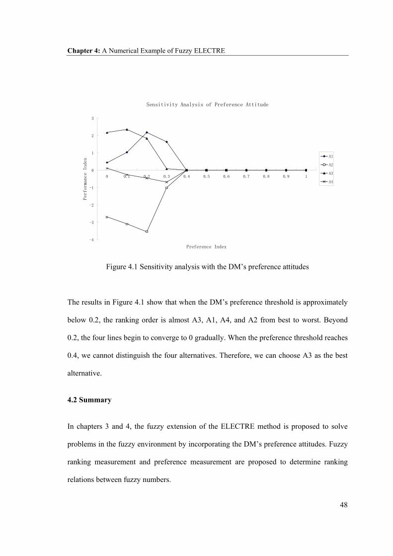
Table 4.16 Performance indices with respect to λ values
λ 0 0.1 0.2 0.3 0.4 0.5 0.6 0.7 0.8 0.9 1.0 A1 0.438 1.032 2.174 1.624 0.000 0.000 0.000 0.000 0.000 0.000 0.000 A2 -2.705 -3.106 -3.542 -1.014 0.000 0.000 0.000 0.000 0.000 0.000 0.000 A3 2.164 2.344 1.828 0.073 0.000 0.000 0.000 0.000 0.000 0.000 0.000 A4 0.102 -0.271 -0.460 -0.683 0.000 0.000 0.000 0.000 0.000 0.000 0.000
Chapter 4: A Numerical Example of Fuzzy ELECTRE
48
Sensitivity Analysis of Preference Attitude
-4
-3
-2
-1
0
1
2
3
0 0.1 0.2 0.3 0.4 0.5 0.6 0.7 0.8 0.9 1
Preference Index
Perfor
mance
Index
A1
A2
A3
A4
Figure 4.1 Sensitivity analysis with the DM’s preference attitudes
The results in Figure 4.1 show that when the DM’s preference threshold is approximately
below 0.2, the ranking order is almost A3, A1, A4, and A2 from best to worst. Beyond
0.2, the four lines begin to converge to 0 gradually. When the preference threshold reaches
0.4, we cannot distinguish the four alternatives. Therefore, we can choose A3 as the best
alternative.
4.2 Summary In chapters 3 and 4, the fuzzy extension of the ELECTRE method is proposed to solve
problems in the fuzzy environment by incorporating the DM’s preference attitudes. Fuzzy
ranking measurement and preference measurement are proposed to determine ranking
relations between fuzzy numbers.

Chapter 4: A Numerical Example of Fuzzy ELECTRE
49
The ELECTRE method is regarded as one of the best MCDM methods because of its
simple logic, full utilization of information and refined computational procedure. Our
proposed fuzzy ELECTRE method provides an efficient way to treat the imprecision and
subjectiveness that may arise in the decision process, and it is flexible in solving complex
problems.
In the next two chapters, we will propose a fuzzy MCDM method based on risk and
confidence analysis, followed by an example.

Chapter 5: Fuzzy MCDM Based on Risk and Confidence Analysis
50
Chapter 5
Fuzzy MCDM Based on Risk and Confidence Analysis
In this chapter, we propose a fuzzy MCDM method based on risk and confidence analysis.
First we propose the methods to model the DM’s risk attitude and confidence attitude
towards uncertainty by the linguistic approach. Then we present our detailed fuzzy
MCDM model.
5.1 Introduction
To deal with uncertainty in decision analysis, the human-related, subjective judgment and
interpretation of “uncertainty” is needed (Zimmermann, 2002). Indubitably, the value of
fuzzy MCDM methods will be improved if the human adaptability, intransitivity, and
dynamic adjustment of preferences can be considered in the decision process (Liang,
1999). The DM’s subjective preference and judgment are intuitively involved in the
process of decision analysis. Incorporating the optimism index into fuzzy MCDM is first
proposed by Zeleny (1982). Some other MCDM methods (Cheng and Mon, 1994; Cheng,
1996; Deng, 1999; Yeh and Deng, 1997) also utilize the DM’s confidence interval and
optimism index to evaluate the alternatives.
We (2003a, 2003b, 2003c, 2003d and 2003e) proposed fuzzy MCDM based on risk and
confidence analysis. This method introduces the modeling of confidence attitude and risk

Chapter 5: Fuzzy MCDM Based on Risk and Confidence Analysis
51
attitude towards uncertainty to support normative fuzzy MCDM. In this approach, the
DM’s subjective preference, judgment and assessment are incorporated into decision
process. Thus, it provides an effective way to solve complex, ill-defined and human-
oriented MCDM problems.
This method uses fuzzy numbers and the linguistic approach to establish risk and
confidence analysis into the multiple criteria decision model. The linguistic approach is
first introduced in section 5.2, and in section 5.3, we will introduce the linguistic modeling
of risk and confidence attitude and the proposed fuzzy MCDM model based on risk and
confidence analysis.
5.2 Modeling of Linguistic Approach
Fuzzy set theory is useful in processing linguistic information. The linguistic approach is
an effective way of expressing the DM’s subjectiveness under different decision situations.
It is used in situations in which the problem is too complex or too ill-defined. By using a
vector-valued objective function, it provides a language for an approximate linguistic
characterization of the trade-offs between its components. The central concept of the
linguistic approach is the linguistic variable. A linguistic variable can be regarded either as
a variable whose value is a fuzzy number or as a variable whose values are defined in
linguistic terms. By means of linguistic variables, the membership functions of fuzzy
number are processed accordingly. Linguistic terms have been intuitively used in
expressing the subjectiveness and imprecision of the DM’s assessments (Zadeh, 1975;
Deng and Yeh, 1998; Liang, 1999). The basic definitions are as follows.

Chapter 5: Fuzzy MCDM Based on Risk and Confidence Analysis
52
Definition 5.1: A linguistic variable is characterized by a quintuple ( x , )(xT , U , G , M~ )
in which x is the name of the variable; )(xT (or simply )(T ) denotes the term set of x ,
that is, the set of names of linguistic values of x , with each value being a fuzzy variable
denoted generically by X and ranging over a universe of discourse U that is associated
with the base variable u ; G is a syntactic rule for generating the name, X , of values of
x ; and M is a semantic rule for associating with each X its meaning, )(~ xM , which is a
fuzzy subset of U . Any X , generated by G , is called a term. Often the name of the
variable and the generic name of the elements of the variable are denoted by the same
symbol. The same holds for X and M~ .
Definition 5.2: A linguistic variable x is called termed if )(xT and the meaning )(~ xM
can be regarded as algorithms that generate the terms of the term set and associate
meanings with them.
Definition 5.3: A linguistic hedge or a modifier is an operation that changes the meaning
of a term or more generally, of a fuzzy set. If A~ is a fuzzy set, its modifier m generates
the term )~(~ AmB = .
Mathematical models frequently used for modifiers are as follows:
a. Concentration:
2~)~( ))(()( xx AAcon µµ = .
b. Dilation:
21~)~( ))(()( xx AAdil µµ = .

Chapter 5: Fuzzy MCDM Based on Risk and Confidence Analysis
53
c. Contrast intensification:
−−∈
=.,))(1(21
],5.0,0[)(,))((2)( 2
~
~2
~
)~int( otherwisexxx
xA
AAA µ
µµµ
5.3 The Proposed Method
Interval information is common in uncertain situations (Moore, R.E. 1979; Neumaier, A.,
1990; Alefeld, G., Mayer, G., 1996). An interval number is based on a two-value
judgment: the minimum possible value and the maximum possible value. In our proposed
method, we use the interval number to represent the uncertain rating of alternatives and
weights of criteria in the MCDM problem.
For the DM’s risk attitude towards uncertainty, the optimist tends to feel that the
uncertainty will be resolved in a favorable manner and the pessimist tends to feel that the
uncertainty will be resolved in an unfavorable manner (Yager, 2000). In the case of risk
attitude to interval assessments, optimism (absolute) means a higher preference to superior
value, while pessimism (absolute) means a higher preference to inferior value. Next,
another kind of subjectiveness we deal with is the DM’s confidence in the fuzzy
assessments. More confidence means that the DM will give a higher preference to the
values with a higher possibility and a lower preference to the values with a lower
possibility. For the confidence attitude to a triangular fuzzy number, more confidence
means assessment towards uncertainty is closer to the modal value. Naturally the DM’s
risk attitudes and confidence attitudes are vague in complex and ill-defined situations.
Linguistic terms are intuitively used to express these attitudes.
Chapter 5: Fuzzy MCDM Based on Risk and Confidence Analysis
54
5.3.1 Modeling of Risk Attitudes
Interval arithmetic is introduced in detail by Moore (1979) and Neumaier (1990). We
define an interval number and its arithmetic operations as follows:
Definition 5.4: An interval number A is defined by a closed interval ],[ supinf aa .
Let ],[ supinf aaA = and ],[ supinf bbB = be two positive interval numbers ( 0inf >a
and 0inf >b ). The basic arithmetic operators are defined as:
a. Negation: ],[ infsup aaA −−=− .
b. Inversion: ]1,1[ infsup1 aaA =− .
c. Addition: ],[ supsupinfinf babaBA ++=+ .
d. Subtraction: ],[ infsupsupinf babaBA −−=− .
e. Multiplication: ],[ supsupinfinf babaBA = .
f. Division: ],[ infsupsupinf babaBA = . (5.1)
For the risk attitude towards the interval number expressed by a superior value and an
inferior value, optimism (absolute) means a higher preference to the superior value, while
pessimism (absolute) means a higher preference to the inferior value. A linguistic variable
“risk attitude” is defined as a mathematical model. Here linguistic terms we use are
absolutely optimism (AO), very optimism (VO), optimism (O), fairly optimism (FO),
neutral (N), fairly pessimism (FP), pessimism (P), very pessimism (VP), and absolutely
pessimism (AP) to represent the decision maker’s qualitative assessments. The number

Chapter 5: Fuzzy MCDM Based on Risk and Confidence Analysis
55
nine is based on Miller’s theory (1956) that seven plus or minus two represents the great
amount of information that the DM can express on the basis of a subjective judgment.
Definition 5.5: T (Risk Attitude) = {AO, VO, O, FO, N, FP, P, VP, AP}.
Fuzzy numbers are intuitively easy and effective in expressing the DM’s qualitative
assessments (Liang, 1999; Yeh and Deng, 2000; Chen, 2000; Cheng, 2002). Here we
propose triangular fuzzy numbers to express linguistic terms of risk attitudes to the
interval uncertainty. With the reference of the inferior value and superior value as the
lower value and upper value of the support boundary, respectively, the modal values are
taken in an average distribution with respect to the optimism (pessimism) attitudes
accordingly. Thus, we define the triangular fuzzy numbers to represent optimism
(pessimism) attitude towards risk as:
Definition 5.6: To express the decision attitude to an interval ],[ supinf aaA = , a triangular
fuzzy number is defined as:
A~ = ( 1a , 2a , 3a ) , (5.2)
where
inf1 aa = , sup
3 aa = , and 8)1)(( infsupinf2 −−+= xaaaa , =x 1, 2, …, 9 represent the
linguistic terms AP, VP, P, FP, N, FO, O, VO, and AO, respectively.

Chapter 5: Fuzzy MCDM Based on Risk and Confidence Analysis
56
By this method, we incorporate the DM’s risk attitudes into interval assessments. The
linguistic terms of risk attitudes expressed by triangular fuzzy numbers are presented in
Table 5.1 and Figure 5.1.
Table 5.1 Linguistic terms of risk attitude
Linguistic term Triangular Fuzzy number Absolutely optimism (AO) ),,( supsupinf aaa
Very optimism (VO) ),8)7(,( supsupinfinf aaaa +
optimism (O) ),4)3(,( supsupinfinf aaaa +
Fairly optimism (FO) ),8)53(,( supsupinfinf aaaa +
Neutral (N) ),2)(,( supsupinfinf aaaa +
Fairly pessimism (FP) ),8)35(,( supsupinfinf aaaa +
pessimism (P) ),4)3(,( supsupinfinf aaaa +
Very pessimism (VP) ),8)7(,( supsupinfinf aaaa +
Absolutely pessimism (AP) ),,( supinfinf aaa
Figure 5.1 Linguistic terms of risk attitude
X
)(~ xAµ
0infa supa
AOVOOFONFPPVPAP1

Chapter 5: Fuzzy MCDM Based on Risk and Confidence Analysis
57
5.3.2 Modeling of Confidence Attitudes
In assessing the uncertainty of the fuzzy numbers, we need to analyze the confidence of
the DM to the truth or reliability. The interval of confidence (A. Kaufmann and M.M.
Gupta, 1985) is a way to incorporate the confidence attitude into fuzzy numbers. Some
MCDM methods (Cheng and Mon, 1994; Cheng, 1996; Deng, 1999; Yeh and Deng, 1997)
have used confidence interval concepts to evaluate the alternatives. However, this
confidence interval cannot fully incorporate the DM’s confidence towards the uncertainty.
A fuzzy number on confidence is more effective on this matter.
We propose a method to express the DM’s confidence on fuzzy numbers. More
confidence means that the DM’s assessment is closer to the most likely value. In the case
of a triangular fuzzy number, this means that the DM’s assessment is closer to the modal
value. Therefore, we define a modified triangular fuzzy number based on the α-cut
concept to incorporate the DM’s confidence assessment to the uncertainty as:
Definition 5.7: Assuming that confidence to the triangular fuzzy number A~ = ( 1a , 2a , 3a )
is at level α , the refined fuzzy number on confidence level is defined as:
))(,),(())(,),((~2332121321 aaaaaaaaaaA −−−+== ααααα , ]1,0[∈α . (5.3)
Figure 5.2 shows a triangular fuzzy number and its corresponding α-cut triangular fuzzy
number.
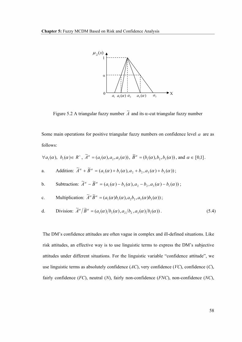
Chapter 5: Fuzzy MCDM Based on Risk and Confidence Analysis
58
Figure 5.2 A triangular fuzzy number A~ and its α-cut triangular fuzzy number
Some main operations for positive triangular fuzzy numbers on confidence level α are as
follows:
),(1 αa∀ +∈ Rb )(1 α , ))(,),((~321 ααα aaaA = , ))(,),((~
321 ααα bbbB = , and ]1,0[∈α .
a. Addition: ))()(,),()((~~332211 αααααα bababaBA +++=+ ;
b. Subtraction: ))()(,),()((~~132231 αααααα bababaBA −−−=− ;
c. Multiplication: ))()(,),()((~~332211 αααααα bababaBA = ;
d. Division: ))()(,,)()((~~132231 αααααα bababaBA = . (5.4)
The DM’s confidence attitudes are often vague in complex and ill-defined situations. Like
risk attitudes, an effective way is to use linguistic terms to express the DM’s subjective
attitudes under different situations. For the linguistic variable “confidence attitude”, we
use linguistic terms as absolutely confidence (AC), very confidence (VC), confidence (C),
fairly confidence (FC), neutral (N), fairly non-confidence (FNC), non-confidence (NC),
X
1
0 )(1 αa
α
1a 2a 3a)(3 αa
)(~ xAµ

Chapter 5: Fuzzy MCDM Based on Risk and Confidence Analysis
59
very non-confidence (VNC), and absolutely non-confidence (ANC) to represent the DM’s
qualitative assessments. We define these linguistic terms as:
Definition 5.8: T (Confidence Attitude) = {AC, VC, C, FC, N, FNC, NC, VNC, ANC}.
Using the confidence level α in the interval [0, 1], we define the membership function of
the linguistic terms of “confidence attitude” to express the DM’s subjective confidence.
Obviously, the membership degree of confidence will increase linearly when α increases
from 0 to 1. Thus, we can use a linear function to represent it and other confidence terms
can be defined by the concentration, dilation and contrast intensification operations,
accordingly.
Definition 5.9: The linguistic terms and their corresponding membership functions are
defined in Table 5.2 and shown in Figure 5.3.
Table 5.2 Linguistic terms of confidence attitude
Linguistic term Membership function
Absolutely confidence (AC) =
=otherwiseAC ,0
1,1)(
ααµ , ]1,0[∈α .
Very confidence (VC) 22))(()( ααµαµ == CVC , ]1,0[∈α .
Confidence (C) ααµ =)(C , ]1,0[∈α .
Fairly confidence (FC) ααµαµ == 5.0))(()( CFC , ]1,0[∈α .
Neutral (N) ,1)( =αµU ]1,0[∈α .
Fairly non-confidence (FNC) ααµαµ −=−= 1))(1()( 5.0CFNC , ].1,0[∈α
Non-confidence (NC) ααµαµ −=−= 1)(1)( CNC , ]1,0[∈α .
Very non-confidence (VNC) ,)1())(1()( 22 ααµαµ −=−= CVNC ]1,0[∈α .
Absolutely non-confidence (ANC) =
=otherwiseANC ,0
0,1)(
ααµ , ]1,0[∈α .

Chapter 5: Fuzzy MCDM Based on Risk and Confidence Analysis
60
0 0.2 0.4 0.6 0.8 10
0.1
0.2
0.3
0.4
0.5
0.6
0.7
0.8
0.9
1
C
FC
VC
NC
FNC
VNC
ANC AC
N
Figure 5.3 Linguistic terms of confidence attitude
Based on the definition above, there are four basic properties of the linguistic terms of
confidence attitude:
a. nvery)( confidence → absolutely confidence as ∞→n ;
b. nvery)( non-confidence → absolutely non-confidence as ∞→n ;
c. nfairly)( confidence → neutral as ∞→n ;
d. nfairly)( non confidence → neutral as ∞→n .
We still need to compare, evaluate and aggregate the performance of the alternatives on
the confidence levels. Therefore, a vector method is proposed here. According to the
membership function of the linguistic term, the confidence membership value is
determined with respect to the confidence level. We define the confidence vector as:

Chapter 5: Fuzzy MCDM Based on Risk and Confidence Analysis
61
Definition 5.10: Assume that there is a total of l ( 2≥l ) confidence levels. The
confidence vector is defined as:
( )lkLT cccC KK ,,1= , (5.5)
where
)(αµLTkc = , 11−
−= lkα , ,,...,2,1 lk = 2≥l , and LT represents linguistic terms AC,
VC, C, FC, N, FNC, NC, VNC, and ANC, respectively.
The selection of l is rather arbitrary. The larger the l , the more calculation is needed, but
a closer to real confidence membership function is achieved. We need a normalized scale
for comparable calculation. Therefore, a normalized format is defined as:
Definition 5.11: The normalized confidence vector is defined as:
( )***1
* ,, lkLT cccC KK= , (5.6)
where
∑ ==
l
k kkk ccc1
* , and symbol kc has the same meaning as equation (5.5).
For the linguistic terms defined in Table 5.2, the corresponding confidence vectors are
obtained as follows:
(1) Absolutely Confidence Vector:
( )1,,0,,0* KK=ACC . (5.7)

Chapter 5: Fuzzy MCDM Based on Risk and Confidence Analysis
62
(2) Very Confidence Vector:
−−−
−=
∑=
1,,)1
1(
)11(
,,0
1
2
2* KK l
k
VC
lk
lk
C . (5.8)
(3) Confidence Vector:
−−
−−−
−=
∑∑==
l
k
l
k
C
lk
lk
lk
C
11
*
)11(
1,,)1
1(
11
,,0 KK . (5.9)
(4) Fairly Confidence Vector:
−−
−−
−−
=
∑∑==
l
k
l
k
FC
lk
lk
lk
C
11
*
)11(
1,,)1
1(
11
,,0 KK . (5.10)
(5) Neutral vector:
( )lllCN1,,1,,1* KK= . (5.11)
(6) Fairly Non-Confidence Vector:
−−−
−−−
−−−
=
∑∑==
0,,
111
111
,,
111
1
11
* KK l
k
l
k
FNC
lk
lk
lk
C . (5.12)

Chapter 5: Fuzzy MCDM Based on Risk and Confidence Analysis
63
(7) Non-Confidence Vector:
−−−
−−−
−−−
=
∑∑==
0,,)1
11(
111
,,)1
11(
1
11
* KK l
k
l
k
NC
lk
lk
lk
C . (5.13)
(8) Very Non-Confidence Vector:
−−−
−−−
−−−
=
∑∑==
0,,)1
11(
)111(
,,)1
11(
12
1
2
1
2
* KK l
k
l
k
VNC
lk
lk
lk
C . (5.14)
(9) Absolutely Non-Confidence Vector:
( )0,,0,,1* KK=ACC . (5.15)
5.3.3 Proposed Fuzzy MCDM based on Risk and Confidence Analysis
Fuzzy MCDM models are typically based on a two-phase approach (Zimmermann, 1987;
Chen and Hwang, 1992; Munda et al., 1995; Ribeiro, 1996). The first phase is to
aggregate the performance of the ratings of alternatives under criteria. Usually triangular
fuzzy numbers are used to express the DM’s assessments on the alternatives’ performance
in terms of each criterion. After the criteria are weighted, the fuzzy utilities represented by
fuzzy numbers are aggregated by fuzzy arithmetic (Kaufmanns and Gupta, 1991). The
second phase is to rank alternatives with respect to the aggregated performances. This
involves the ranking of the alternatives based on the comparison of their corresponding
fuzzy utilities.

Chapter 5: Fuzzy MCDM Based on Risk and Confidence Analysis
64
In the second phase of fuzzy MCDM analysis, ranking of fuzzy numbers is a hard task.
Though many methods have been proposed, the computation is complex and unreliable.
This is because the comparison process may (a) involve considerable computations, (b)
produce inconsistent outcomes by different fuzzy ranking methods, and (c) generate
counter-intuitive ranking outcomes for similar fuzzy utilities (Bortolan and Degani, 1985;
Zimmermann, 1987; Chen and Hwang, 1992; Chen and Klien, 1997). In our method, with
reference to the imaged ideal alternative solutions, fuzzy numbers are aggregated into
crisp performance in the second phase. Thus it makes the computation efficient and avoids
the complicated and unreliable fuzzy number ranking.
We propose this approach to solve the fuzzy MCDM problems by incorporating the DM’s
risk attitude and confidence attitude. Interval numbers are used to assess the ratings of
alternatives and the weights of criteria. The decision matrix is transformed into a
performance matrix representing a weighted interval assessment. Risk attitudes are
incorporated by triangular fuzzy numbers. Based on the α-cut concept, the fuzzy numbers
are incorporated with confidence levels. According to the concept of ideal solutions, we
define the fuzzy ideal solutions as: fuzzy positive ideal solution and fuzzy negative ideal
solution. Then we measure the degree of separation of fuzzy numbers by the vertex
method. The degree of separation transforms fuzzy performance into a crisp performance
under confidence levels. According to the confidence attitudes, we obtain confidence
vectors with respect to the membership functions. Finally, by aggregating performance
values under confidence levels, the overall performance is obtained to evaluate the
alternatives. We give the procedure as follows:

Chapter 5: Fuzzy MCDM Based on Risk and Confidence Analysis
65
Step 1: Problem Formulation
For conciseness, fuzzy MCDM can be expressed in the matrix format as:
=
mnmm
n
n
xxx
xxxxxx
D
K
KKKK
K
K
21
22221
11211
, (5.16)
),,,( 21 nwwwW K= , (5.17)
where
ijx and jw ( =i 1, 2, ,K m ; =j 1, 2, ,K n ) are positive interval numbers. ijx is the rating
of alternative iA with respect to criterion jC , and it forms a matrix referred to as the
decision matrix. jw is the weight of criterion jC , and it forms a vector referred to as the
weighting vector.
Step 2: Construct the Performance Matrix
Considering the importance of each criterion, we construct the fuzzy performance matrix
by multiplying the weighting vector by the decision matrix, using the interval
multiplication arithmetic operation.
)],[( supinf
21
22221
11211
ijij
mnmm
n
n
pp
ppp
pppppp
P =
=
K
KKKK
K
K
, =i 1, 2, ,K m , =j 1, 2, ,K n , (5.18)
where infinfinfijjij xwp = and supsupsup
ijjij xwp = .
This process transforms the fuzzy decision matrix into a weighted fuzzy decision matrix,
referred to as the performance matrix.
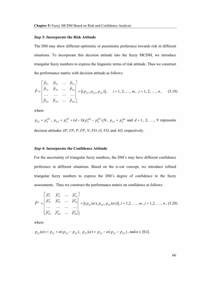
Chapter 5: Fuzzy MCDM Based on Risk and Confidence Analysis
66
Step 3: Incorporate the Risk Attitude
The DM may show different optimistic or pessimistic preference towards risk in different
situations. To incorporate this decision attitude into the fuzzy MCDM, we introduce
triangular fuzzy numbers to express the linguistic terms of risk attitude. Thus we construct
the performance matrix with decision attitude as follows:
)],,[(
~~~
~~~~~~
~321
21
22221
11211
ijijij
mnmm
n
n
ppp
ppp
pppppp
P =
=
K
KKKK
K
K
, =i 1, 2, ,K m , =j 1, 2, ,K n , (5.19)
where
inf1 ijij pp = , 8))(1( infsupinf
2 ijijijij ppdpp −−+= , sup3 ijij pp = and =d 1, 2, …, 9 represents
decision attitudes AP, VP, P, FP, N, FO, O, VO, and AO, respectively.
Step 4: Incorporate the Confidence Attitude
For the uncertainty of triangular fuzzy numbers, the DM’s may have different confidence
preference in different situations. Based on the α-cut concept, we introduce refined
triangular fuzzy numbers to express the DM’s degree of confidence to the fuzzy
assessments. Thus we construct the performance matrix on confidence as follows:
))](,),([(
~~~
~~~~~~
~321
21
22221
11211
αα
ααα
ααα
ααα
αijijij
mnmm
n
n
ppp
ppp
pppppp
P =
=
K
KKKK
K
K
, =i 1,2, ,K m , =j 1,2, ,K n , (5.20)
where
)()( 1211 ijijijij pppp −+= αα , )()( 2333 ijijijij pppp −−= αα , and ]1,0[∈α .

Chapter 5: Fuzzy MCDM Based on Risk and Confidence Analysis
67
The values of α express confidence levels in assessment of the uncertainty of triangular
fuzzy numbers. A larger value means a higher confidence toward uncertainty.
Step 5: Normalization
Generally criteria are incommensurate. The normalization process aims at obtaining
comparable scales. Two main methods, namely vector normalization and linear scale
normalization, are usually used in MCDM (Hwang and Yoon, 1981). Vector
normalization cannot guarantee a criterion scale with an equal length. Linear scale
normalization uses the ways in which the relative outcomes are equal. Moreover, linear
scale normalization is often used for its simplicity. Thus, we will use linear scale
normalization here.
We normalize the fuzzy numbers in the performance matrix on confidence level α as
follows:
=
nmnnmnm
nnnn
nnnn
n
ppp
pppppp
P
ααα
ααα
ααα
α
~~~
~~~~~~
~
21
22221
11211
K
KKKK
K
K
, =i 1, 2, ,K m , =j 1, 2, ,K n , (5.21)
where
∈=
∈==
.),(min),)(
,,)(
(
.),(max),)(
,,)(
(~
1123
3321
CjpNp
NpN
pN
BjpMM
pMp
Mp
piji
ijijij
iji
ijijij
nijα
αα
ααα
α
Here B and C represent benefit criteria and cost criteria, respectively. For benefit criteria,
the DM wants to have a maximum value among the alternatives. For cost criteria, the DM

Chapter 5: Fuzzy MCDM Based on Risk and Confidence Analysis
68
wants to have a minimum value among the alternatives. This method preserves the ranges
of normalized triangular fuzzy numbers to be [0, 1].
Step 6: Determine the Positive Ideal and Negative Ideal Solutions
The ideal solution in decision analysis means the desired decision outcome in a given
decision situation. The positive (negative) ideal solution consists of the best (or worst)
criteria values attainable from all the alternatives if each criterion takes monotonically
increasing or decreasing values. The most preferred alternative should have the shortest
distance from the positive ideal solution and the longest distance from the negative ideal
solution (Hwang and Yoon, 1981; Zeleny, 1982). This concept has been widely used in
developing various methodologies for solving practical decision problems (Shipley,
DeKorvin and Obid, 1991; Yeh and Deng, 1997, 1999) due to: (a) its simplicity and
comprehensibility in concept, (b) its computation efficiency, and (c) its ability to measure
the relative performance of the alternatives in a simple mathematical form.
In line with this concept, in the normalized fuzzy performance matrix where its element is
the normalized positive triangular fuzzy number, we can define the fuzzy positive ideal
solution ( *~A ) and fuzzy negative ideal solution ( −A~ ). These two ideal alternatives are
used as references to measure the alternatives’ performance. We determine the positive
ideal solution and the negative ideal solution as follows:
)~,,~,~(~ **2
*1
*npppA K= ,
)~,,~,~(~21
−−−− = npppA K , (5.22)
where

Chapter 5: Fuzzy MCDM Based on Risk and Confidence Analysis
69
=*~jp (1, 1, 1),
=−jp~ (0, 0, 0), =j 1, 2, ,K n .
Step 7: Measure the Separations
The distance of each alternative to the ideal solutions is measured by the vertex method
(Chen, 2000). The vertex method measures distance between two triangular fuzzy
numbers. It avoids the complexity of ranking fuzzy numbers.
The distance between each alternative and the positive ideal solution is calculated as:
∑=
=n
jjniji ppdd
1
** ),~,~( αα =i 1, 2, ,K m , (5.23)
where
2123
22
21
* }3])1()1()1[({)~,~( −+−+−=nijnijnijjnij pppppd αααα ;
The distance between each alternative and the negative ideal solution is calculated as:
∑=
−−=
n
jjniji ppdd
1
),~,~( αα =i 1, 2, ,K m , (5.24)
where
2123
22
21 }3])0()0()0[({)~,~( −+−+−=−
nijnijnijjnij pppppd αααα .
The smaller the value of *α
id and −α
id , the higher the degree of similarity between each
alternative and the positive ideal solution and the negative ideal solution, respectively.

Chapter 5: Fuzzy MCDM Based on Risk and Confidence Analysis
70
Step 8: Determine the Performance on Confidence Level
A preferred alternative should have a higher degree of similarity to the positive ideal
solution, and at the same time have a lower degree of similarity to the negative ideal
solution (Hwang and Yoon, 1981; Zeleny, 1982; Shipley, deKorvin, and Obid, 1991; Yeh
and Deng, 1997, 1999). We prefer the alternative with a lower distance to the positive
ideal solution ( *id ) and a higher distance to the negative ideal solution ( −
id ). Therefore,
an overall performance index for each alternative on confidence level α with respect to
the positive ideal solution and the negative ideal solution is defined as:
)]([21 *ααα
iii dndn
p −+=−
, =i 1, 2, ,K m , (5.25)
where n is the number of criteria.
Obviously, the nearer αip is to 1 means the better the performance of alternative iA ( =i 1,
2, ,K m ).
The alternatives usually have different performance values on different confidence levels.
Assuming that we take a total of l confidence levels that are equally distributed in the
interval [0, 1], we need to obtain all the performance values of alternatives on these levels.
Referring to (5.5), we define a performance vector with respect to the confidence levels as:
( )ilikii pppP KK,,1= , =i 1, 2, ,K m , (5.26)
where αiik pp = , 1
1−
−= lkα , =k 1, 2, ,K l ( 2≥l ).
Chapter 5: Fuzzy MCDM Based on Risk and Confidence Analysis
71
Step 9: Determine the Performance on Confidence Attitude
We use linguistic terms as absolutely confidence (AC), very confidence (VC), confidence
(C), fairly confidence (FC), neutral (N), fairly non-confidence (FNC), non-confidence
(NC), very non-confidence (VNC), and absolutely non-confidence (ANC) to represent the
DM’s confidence attitude. According to the membership functions (Table 5.2), we
determine the confidence vectors from (5.7) to (5.15). The performance of the alternatives
with respect to confidence attitude is obtained as:
∑=
==l
kkik
TLTi
LTi cpCPP
1
* )( , =i 1, 2, ,K m , (5.27)
where
LT represents linguistic terms as AC, VC, C, FC, N, FNC, NC, VNC, and ANC,
respectively.
In summarizing the discussion above, we present the steps for the approach developed as
follows:
Step 1: Formulate the problem in the decision matrix and weighting vector as expressed in
(5.16) and (5.17).
Step 2: Construct the fuzzy performance matrix expressed in (5.18) by multiplying the
weighting vector by the decision matrix.
Step 3: Obtain the DM’s risk attitude in definition 5.5 and construct the performance
matrix with risk attitude in (5.19).
Step 4: Construct the performance matrix on confidence level as expressed in (5.20).
Step 5: Normalize the performance matrix by (5.21) to get comparable scales.
Chapter 5: Fuzzy MCDM Based on Risk and Confidence Analysis
72
Step 6: Determine the positive ideal solution and the negative ideal solution by (5.22). The
positive ideal solution and the negative ideal solution are used as references to measure
the alternatives’ performance.
Step 7: Measure the separations of the alternatives to the ideals solutions by (5.23) and
(5.24).
Step 8: Determine the performance on confidence level by (5.25). Take a total of l
confidence levels as denoted in (5.5) and calculate the performance vector with respect to
confidence levels as expressed in (5.26).
Step 9: According to the DM’s confidence attitudes in definition 5.8, determine the
confidence vectors and calculate the alternatives’ performance by (5.27). The DM ranks,
selects or prioritizes the alternatives according to their performance index values.
In the following chapter, we will give a numerical example to illustrate the computation
process.

Chapter 6: A Numerical Example of Fuzzy MCDM Based on Risk and Confidence Analysis
73
Chapter 6
A Numerical Example of Fuzzy MCDM Based on Risk and
Confidence Analysis
In this chapter, we give a numerical example to illustrate the computation process of fuzzy
MCDM based on risk and confidence analysis.
6.1 A Step-by-step Approach
We illustrate our method by a MCDM problem with four alternatives under four benefit
criteria. In the following, we consider absolutely optimism (AO) attitude towards risk in
the solving process.
Step 1: Problem Formulation
The decision matrix and the weighting vector of the problem are given in Table 6.1.
Table 6.1 Decision matrix and weighting vector
C1 C2 C3 C4 [0.10 0.30] [0.20 0.40] [0.30 0.50] [0.05 0.15] A1 [2.00 6.00] [3.00 7.00] [3.00 8.00] [4.00 9.00] A2 [2.00 7.00] [3.00 7.00] [1.00 5.00] [4.00 8.00] A3 [5.00 9.00] [1.00 8.00] [2.00 7.00] [4.00 9.00] A4 [1.00 5.00] [3.00 6.00] [5.00 9.00] [7.00 9.00]

Chapter 6: A Numerical Example of Fuzzy MCDM Based on Risk and Confidence Analysis
74
Step 2: Construct the Performance Matrix
The performance matrix is constructed in Table 6.2.
Table 6.2 Performance matrix
C1 C2 C3 C4 A1 [0.20 1.80] [0.60 2.80] [0.90 4.00] [0.20 1.35] A2 [0.20 2.10] [0.60 2.80] [0.30 2.50] [0.20 1.20] A3 [0.50 2.70] [0.20 3.20] [0.60 3.50] [0.20 1.35] A4 [0.10 1.50] [0.60 2.40] [1.50 4.50] [0.35 1.35]
Step 3: Incorporate the Risk Attitude
The performance matrix is incorporated with absolutely optimism attitude in Table 6.3.
Table 6.3 Performance matrix under AO attitude
C1 C2 C3 C4 A1 (0.20, 1.80, 1.80) (0.60, 2.80, 2.80) (0.90, 4.00, 4.00) (0.20, 1.35, 1.35) A2 (0.20, 2.10, 2.10) (0.60, 2.80, 2.80) (0.30, 2.50, 2.50) (0.20, 1.20, 1.20) A3 (0.50, 2.70, 2.70) (0.20, 3.20, 3.20) (0.60, 3.50, 3.50) (0.20, 1.35, 1.35) A4 (0.10, 1.50, 1.50) (0.60, 2.40, 2.40) (1.50, 4.50, 4.50) (0.35, 1.35, 1.35)
Step 4: Incorporate the Confidence Attitude
Taking a total of 11 ( 1,,1.0,0 K=α ) confidence levels, we construct the performance
matrix on confidence. The performance matrix under AO on 0.5 confidence level is
presented in Table 6.4.
Table 6.4 Performance matrix under AO attitude when α=0.5
C1 C2 C3 C4 A1 (1.00, 1.80, 1.80) (1.70, 2.80, 2.80) (2.45, 4.00, 4.00) (0.78, 1.35, 1.35) A2 (1.15, 2.10, 2.10) (1.70, 2.80, 2.80) (1.40, 2.50, 2.50) (0.70, 1.20, 1.20) A3 (1.60, 2.70, 2.70) (1.70, 3.20, 3.20) (2.05, 3.50, 3.50) (0.78, 1.35, 1.35) A4 (0.80, 1.50, 1.50) (1.50, 2.40, 2.40) (3.00, 4.50, 4.50) (0.85, 1.35, 1.35)

Chapter 6: A Numerical Example of Fuzzy MCDM Based on Risk and Confidence Analysis
75
Step 5: Normalization
The normalized performance matrix under AO on 0.5 confidence level is presented in
Table 6.5.
Table 6.5 Normalized performance matrix under AO attitude when α=0.5
C1 C2 C3 C4 A1 (0.370, 0.667, 0.667) (0.531, 0.875, 0.875) (0.544, 0.889, 0.889) (0.574, 1.000, 1.000) A2 (0.426, 0.778, 0.778) (0.531, 0.875, 0.875) (0.311, 0.556, 0.556) (0.519, 0.889, 0.889) A3 (0.593, 1.000, 1.000) (0.531, 1.000, 1.000) (0.456, 0.778, 0.778) (0.574, 1.000, 1.000) A4 (0.296, 0.556, 0.556) (0.469, 0.750, 0.750) (0.667, 1.000, 1.000) (0.630, 1.000, 1.000)
Step 6: Determine the Positive Ideal and Negative Ideal Solutions
The alternatives’ separation distance to the positive ideal solution and the negative ideal
solution are calculated in Table 6.6.
Table 6.6 Separation distance under AO when α=0.5
C1 C2 C3 C4 Overall P N P N P N P N P N
A1 0.454 0.585 0.289 0.778 0.278 0.791 0.246 0.881 1.268 3.034 A2 0.378 0.681 0.289 0.778 0.538 0.488 0.292 0.785 1.498 2.732 A3 0.235 0.885 0.271 0.872 0.363 0.687 0.246 0.881 1.115 3.326 A4 0.545 0.485 0.368 0.670 0.193 0.903 0.214 0.894 1.320 2.951
Step 7: Measure the Separations
The performance indices under 11 confidence levels are calculated in Table 6.7 and shown
in Figure 6.1. We can clearly observe how the alternatives’ performance values vary with
the confidence level in the figure.

Chapter 6: A Numerical Example of Fuzzy MCDM Based on Risk and Confidence Analysis
76
Table 6.7 Performance index under AO with 11 confidence levels
Confidence level 0 0.1 0.2 0.3 0.4 0.5 0.6 0.7 0.8 0.9 1.0
A1 0.598 0.621 0.644 0.669 0.695 0.721 0.748 0.775 0.803 0.831 0.858 A2 0.544 0.564 0.586 0.608 0.631 0.654 0.678 0.703 0.727 0.751 0.774 A3 0.633 0.659 0.687 0.716 0.745 0.776 0.809 0.841 0.875 0.910 0.944 A4 0.595 0.615 0.636 0.658 0.681 0.704 0.728 0.752 0.777 0.801 0.826
0 0.2 0.4 0.6 0.8 10.5
0.55
0.6
0.65
0.7
0.75
0.8
0.85
0.9
0.95
Confidence Value
Per
form
ance
val
ue
Confidence Level Sensitivity Analysis
← A1
← A2
← A3
← A4
Figure 6.1 Performance value under AO with respect to confidence levels
Step 8: Determine the Performance on Confidence Level
According to the DM’s confidence attitudes, we take a total of 11 levels to calculate the
confidence vectors. The entries in the vectors are presented in Table 6.8.

Chapter 6: A Numerical Example of Fuzzy MCDM Based on Risk and Confidence Analysis
77
Table 6.8 Confidence vector under 11 confidence levels
Confidence vector 1 2 3 4 5 6 7 8 9 10 11
AC 0.000 0.000 0.000 0.000 0.000 0.000 0.000 0.000 0.000 0.000 1.000 VC 0.000 0.003 0.010 0.023 0.042 0.065 0.094 0.127 0.166 0.210 0.260 C 0.000 0.018 0.036 0.055 0.073 0.090 0.109 0.127 0.145 0.164 0.182 FC 0.000 0.044 0.063 0.077 0.089 0.100 0.109 0.118 0.126 0.134 0.141 N 0.091 0.091 0.091 0.091 0.091 0.091 0.091 0.091 0.091 0.091 0.091 FNC 0.141 0.134 0.126 0.118 0.109 0.100 0.089 0.077 0.063 0.044 0.000 NC 0.182 0.164 0.145 0.127 0.109 0.090 0.073 0.055 0.036 0.018 0.000 VNC 0.260 0.210 0.166 0.127 0.094 0.065 0.042 0.023 0.010 0.003 0.000 ANC 1.000 0.000 0.000 0.000 0.000 0.000 0.000 0.000 0.000 0.000 0.000
Step 9: Determine the Performance on Confidence Attitude
Calculate the alternatives’ performance under AO from absolute confident to absolute non
confident attitudes in Table 6.9.
Table 6.9 Performance index under AO with respect to confidence attitudes
A1 A2 A3 A4 P Order P Order P Order P Order
AC 0.8576 2 0.7743 4 0.9444 1 0.8264 3 VC 0.8001 2 0.7242 4 0.8727 1 0.7744 3 C 0.7685 2 0.6960 4 0.8355 1 0.7456 3 FC 0.7549 2 0.6840 4 0.8188 1 0.7338 3 N 0.7165 2 0.6498 4 0.7736 1 0.6995 3 FNC 0.6845 2 0.6215 4 0.7349 1 0.6714 3 NC 0.6646 2 0.6036 4 0.7117 1 0.6534 3 VNC 0.6501 2 0.5908 4 0.6939 1 0.6413 3 ANC 0.5977 2 0.5438 4 0.6332 1 0.5946 3
Finally, we analyze the results in Table 6.9 and make a ranking order. It is clear that A3 is
the best alternative under absolute optimism attitude with respect to all confidence
attitudes, and the other alternatives ranking order are A1, A4 and A2. Repeating the same
steps, we can evaluate and analyze the alternatives’ performances under other risk
attitudes with respect to confidence attitudes. The data and figures are given as follows.

Chapter 6: A Numerical Example of Fuzzy MCDM Based on Risk and Confidence Analysis
78
Performance under VO Attitude
Table 6.10 Performance index under VO with 11 confidence levels
Confidence level 0 0.1 0.2 0.3 0.4 0.5 0.6 0.7 0.8 0.9 1.0
A1 0.576 0.598 0.622 0.646 0.673 0.700 0.729 0.759 0.791 0.822 0.854 A2 0.522 0.542 0.563 0.585 0.609 0.634 0.659 0.686 0.714 0.742 0.770 A3 0.610 0.635 0.662 0.691 0.723 0.753 0.786 0.822 0.859 0.897 0.936 A4 0.575 0.596 0.617 0.640 0.664 0.689 0.715 0.742 0.770 0.799 0.829
0 0.2 0.4 0.6 0.8 10.5
0.55
0.6
0.65
0.7
0.75
0.8
0.85
0.9
0.95
Confidence Value
Per
form
ance
val
ue
Confidence Level Sensitivity Analysis
← A1
← A2
← A3
← A4
Figure 6.2 Performance value under VO with respect to confidence levels
Table 6.11 Performance index under VO with respect to confidence attitudes
A1 A2 A3 A4 P Order P Order P Order P Order
AC 0.8535 2 0.7697 4 0.9363 1 0.8291 3 VC 0.7883 2 0.7119 4 0.8571 1 0.7688 3 C 0.7546 2 0.6817 4 0.8182 1 0.7376 3 FC 0.7396 2 0.6683 4 0.8001 1 0.7242 3 N 0.6993 2 0.6323 4 0.7534 1 0.6873 3 FNC 0.6645 2 0.6013 4 0.7124 1 0.6559 3 NC 0.6439 2 0.5828 4 0.6887 1 0.6369 3 VNC 0.6283 2 0.5689 4 0.6702 1 0.6233 3 ANC 0.5756 2 0.5217 4 0.6101 1 0.5751 3

Chapter 6: A Numerical Example of Fuzzy MCDM Based on Risk and Confidence Analysis
79
Performance under O Attitude
Table 6.12 Performance index under O with 11 confidence levels
Confidence level 0 0.1 0.2 0.3 0.4 0.5 0.6 0.7 0.8 0.9 1.0
A1 0.552 0.574 0.597 0.622 0.648 0.677 0.708 0.740 0.775 0.812 0.849 A2 0.499 0.518 0.538 0.561 0.585 0.610 0.638 0.667 0.698 0.731 0.765 A3 0.585 0.609 0.635 0.622 0.693 0.725 0.760 0.798 0.838 0.881 0.927 A4 0.554 0.575 0.597 0.620 0.645 0.672 0.700 0.730 0.763 0.797 0.833
0 0.2 0.4 0.6 0.8 10.45
0.5
0.55
0.6
0.65
0.7
0.75
0.8
0.85
0.9
0.95
Confidence Value
Per
form
ance
val
ue
Confidence Level Sensitivity Analysis
← A1
← A2
← A3
← A4
Figure 6.3 Performance value under O with respect to confidence levels
Table 6.13 Performance index under O with respect to confidence attitudes
A1 A2 A3 A4 P Order P Order P Order P Order
AC 0.8489 2 0.7645 4 0.9265 1 0.8327 3 VC 0.7744 2 0.6977 4 0.8383 1 0.7624 3 C 0.7386 2 0.6655 4 0.7975 1 0.7285 3 FC 0.7220 2 0.6507 4 0.7781 1 0.7132 3 N 0.6797 2 0.6128 4 0.7301 1 0.6735 3 FNC 0.6422 2 0.5792 4 0.6866 1 0.6386 3 NC 0.6209 2 0.5601 4 0.6626 1 0.6185 3 VNC 0.6044 2 0.5454 4 0.6435 1 0.6036 3 ANC 0.5522 3 0.4987 4 0.5850 1 0.5543 2

Chapter 6: A Numerical Example of Fuzzy MCDM Based on Risk and Confidence Analysis
80
Performance under FO Attitude
Table 6.14 Performance index under FO with 11 confidence levels
Confidence level 0 0.1 0.2 0.3 0.4 0.5 0.6 0.7 0.8 0.9 1.0
A1 0.528 0.548 0.570 0.594 0.621 0.650 0.682 0.718 0.757 0.799 0.844 A2 0.475 0.493 0.512 0.534 0.558 0.584 0.613 0.645 0.680 0.718 0.759 A3 0.558 0.580 0.604 0.631 0.660 0.693 0.729 0.769 0.813 0.861 0.914 A4 0.533 0.552 0.574 0.598 0.623 0.651 0.682 0.716 0.753 0.794 0.838
0 0.2 0.4 0.6 0.8 10.45
0.5
0.55
0.6
0.65
0.7
0.75
0.8
0.85
0.9
0.95
Confidence Value
Per
form
ance
val
ue
Confidence Level Sensitivity Analysis
← A1
← A2
← A3
← A4
Figure 6.4 Performance value under FO with respect to confidence levels
Table 6.15 Performance index under FO with respect to confidence attitudes
A1 A2 A3 A4 P Order P Order P Order P Order
AC 0.8437 2 0.7586 4 0.9143 1 0.8378 3 VC 0.7581 2 0.6812 4 0.8155 1 0.7550 3 C 0.7200 2 0.6470 4 0.7728 1 0.7181 3 FC 0.7018 2 0.6306 4 0.7522 1 0.7001 3 N 0.6578 3 0.5913 4 0.7031 1 0.6582 2 FNC 0.6174 3 0.5550 4 0.6575 1 0.6195 2 NC 0.5956 3 0.5355 4 0.6334 1 0.5984 2 VNC 0.5785 3 0.5203 4 0.6141 1 0.5822 2 ANC 0.5277 3 0.4751 4 0.5584 1 0.5326 2

Chapter 6: A Numerical Example of Fuzzy MCDM Based on Risk and Confidence Analysis
81
Performance under N Attitude
Table 6.16 Performance index under N with 11 confidence levels
Confidence level 0 0.1 0.2 0.3 0.4 0.5 0.6 0.7 0.8 0.9 1.0
A1 0.503 0.521 0.541 0.564 0.590 0.619 0.653 0.690 0.734 0.783 0.838 A2 0.451 0.467 0.485 0.506 0.528 0.554 0.584 0.618 0.657 0.701 0.752 A3 0.531 0.550 0.572 0.596 0.624 0.656 0.692 0.733 0.781 0.836 0.899 A4 0.510 0.529 0.550 0.573 0.599 0.628 0.661 0.699 0.741 0.790 0.846
0 0.2 0.4 0.6 0.8 10.45
0.5
0.55
0.6
0.65
0.7
0.75
0.8
0.85
0.9
Confidence Value
Per
form
ance
val
ue
Confidence Level Sensitivity Analysis
← A1
← A2
← A3
← A4
Figure 6.5 Performance value under N with respect to confidence levels
Table 6.17 Performance index under N with respect to confidence attitudes
A1 A2 A3 A4 P Order P Order P Order P Order
AC 0.8384 3 0.7522 4 0.8988 1 0.8456 2 VC 0.7389 3 0.6621 4 0.7877 1 0.7468 2 C 0.6984 3 0.6256 4 0.7433 1 0.7064 2 FC 0.6786 3 0.6079 4 0.7215 1 0.6868 2 N 0.6333 3 0.5674 4 0.6722 1 0.6415 2 FNC 0.5900 3 0.5287 4 0.6248 1 0.5984 2 NC 0.5681 3 0.5091 4 0.6011 1 0.5765 2 VNC 0.5508 3 0.4938 4 0.5822 1 0.5592 2 ANC 0.5026 3 0.4513 4 0.5307 1 0.5103 2

Chapter 6: A Numerical Example of Fuzzy MCDM Based on Risk and Confidence Analysis
82
Performance under FP Attitude
Table 6.18 Performance index under FP with 11 confidence levels
Confidence level 0 0.1 0.2 0.3 0.4 0.5 0.6 0.7 0.8 0.9 1.0
A1 0.478 0.493 0.512 0.532 0.557 0.585 0.618 0.658 0.705 0.756 0.815 A2 0.428 0.441 0.457 0.475 0.496 0.521 0.551 0.586 0.628 0.674 0.728 A3 0.503 0.519 0.538 0.559 0.584 0.613 0.648 0.690 0.740 0.796 0.861 A4 0.488 0.505 0.525 0.547 0.573 0.602 0.637 0.678 0.727 0.779 0.842
0 0.2 0.4 0.6 0.8 10.4
0.45
0.5
0.55
0.6
0.65
0.7
0.75
0.8
0.85
0.9
Confidence Value
Per
form
ance
val
ue
Confidence Level Sensitivity Analysis
← A1
← A2
← A3← A4
Figure 6.6 Performance value under FP with respect to confidence levels
Table 6.19 Performance index under FP with respect to confidence attitudes
A1 A2 A3 A4 P Order P Order P Order P Order
AC 0.8150 3 0.7276 4 0.8608 1 0.8416 2 VC 0.7101 3 0.6333 4 0.7472 1 0.7324 2 C 0.6689 3 0.5965 4 0.7034 1 0.6895 2 FC 0.6486 3 0.5785 4 0.6818 1 0.6682 2 N 0.6036 3 0.5386 4 0.6345 1 0.6211 2 FNC 0.5597 3 0.4996 4 0.5880 1 0.5752 2 NC 0.5383 3 0.4807 4 0.5655 1 0.5528 2 VNC 0.5214 3 0.4660 4 0.5480 1 0.5348 2 ANC 0.4775 3 0.4277 4 0.5028 1 0.4878 2

Chapter 6: A Numerical Example of Fuzzy MCDM Based on Risk and Confidence Analysis
83
Performance under P Attitude
Table 6.20 Performance index under P with 11 confidence levels
Confidence level 0 0.1 0.2 0.3 0.4 0.5 0.6 0.7 0.8 0.9 1.0
A1 0.453 0.466 0.481 0.499 0.520 0.546 0.577 0.615 0.658 0.713 0.782 A2 0.405 0.416 0.428 0.443 0.462 0.484 0.512 0.545 0.582 0.630 0.693 A3 0.475 0.488 0.502 0.519 0.540 0.565 0.596 0.634 0.678 0.735 0.807 A4 0.465 0.481 0.498 0.519 0.543 0.573 0.608 0.650 0.698 0.759 0.835
0 0.2 0.4 0.6 0.8 10.4
0.45
0.5
0.55
0.6
0.65
0.7
0.75
0.8
0.85
0.9
Confidence Value
Per
form
ance
val
ue
Confidence Level Sensitivity Analysis
← A1
← A2
← A3← A4
Figure 6.7 Performance value under P with respect to confidence levels
Table 6.21 Performance index under P with respect to confidence attitudes
A1 A2 A3 A4 P Order P Order P Order P Order
AC 0.7821 3 0.6927 4 0.8069 2 0.8354 1 VC 0.6704 3 0.5936 4 0.6919 2 0.7113 1 C 0.6301 3 0.5582 4 0.6509 2 0.6666 1 FC 0.6103 3 0.5409 4 0.6310 2 0.6443 1 N 0.5678 3 0.5039 4 0.5886 2 0.5966 1 FNC 0.5253 3 0.4668 4 0.5459 2 0.5488 1 NC 0.5055 3 0.4497 4 0.5262 2 0.5267 1 VNC 0.4905 3 0.4369 4 0.5118 1 0.5091 2 ANC 0.4527 3 0.4048 4 0.4751 1 0.4654 2

Chapter 6: A Numerical Example of Fuzzy MCDM Based on Risk and Confidence Analysis
84
Performance under VP Attitude
Table 6.22 Performance index under VP with 11 confidence levels
Confidence level 0 0.1 0.2 0.3 0.4 0.5 0.6 0.7 0.8 0.9 1.0
A1 0.429 0.438 0.450 0.463 0.480 0.502 0.528 0.558 0.598 0.653 0.732 A2 0.383 0.390 0.399 0.411 0.425 0.443 0.464 0.489 0.522 0.569 0.639 A3 0.448 0.456 0.466 0.478 0.493 0.511 0.534 0.561 0.597 0.649 0.724 A4 0.444 0.456 0.471 0.490 0.512 0.539 0.572 0.611 0.660 0.728 0.824
0 0.2 0.4 0.6 0.8 10.35
0.4
0.45
0.5
0.55
0.6
0.65
0.7
0.75
0.8
0.85
Confidence Value
Per
form
ance
val
ue
Confidence Level Sensitivity Analysis
← A1
← A2
← A3
← A4
Figure 6.8 Performance value under VP with respect to confidence levels
Table 6.23 Performance index under VP with respect to confidence attitudes
A1 A2 A3 A4 P Order P Order P Order P Order
AC 0.7316 2 0.6388 4 0.7235 3 0.8244 1 VC 0.6169 2 0.5398 4 0.6164 3 0.6828 1 C 0.5797 3 0.5081 4 0.5819 2 0.6372 1 FC 0.5619 3 0.4932 4 0.5661 2 0.6143 1 N 0.5247 3 0.4620 4 0.5325 2 0.5677 1 FNC 0.4864 3 0.4299 4 0.4982 2 0.5190 1 NC 0.4697 3 0.4159 4 0.4831 2 0.4981 1 VNC 0.4581 3 0.4067 4 0.4737 2 0.4820 1 ANC 0.4287 3 0.3828 4 0.4483 1 0.4435 2

Chapter 6: A Numerical Example of Fuzzy MCDM Based on Risk and Confidence Analysis
85
Performance under AP attitude
Table 6.24 Performance index under AP with 11 confidence levels
Confidence level 0 0.1 0.2 0.3 0.4 0.5 0.6 0.7 0.8 0.9 1.0
A1 0.406 0.412 0.419 0.427 0.439 0.454 0.468 0.487 0.516 0.562 0.643 A2 0.362 0.366 0.371 0.377 0.386 0.397 0.407 0.420 0.441 0.476 0.543 A3 0.423 0.426 0.431 0.436 0.443 0.452 0.460 0.471 0.489 0.518 0.576 A4 0.422 0.432 0.444 0.459 0.478 0.502 0.527 0.561 0.609 0.681 0.800
0 0.2 0.4 0.6 0.8 10.35
0.4
0.45
0.5
0.55
0.6
0.65
0.7
0.75
0.8
Confidence Value
Per
form
ance
val
ue
Confidence Level Sensitivity Analysis
← A1
← A2
← A3
← A4
Figure 6.9 Performance value under AP with respect to confidence levels
Table 6.25 Performance index under AP with respect to confidence attitudes
A1 A2 A3 A4 P Order P Order P Order P Order
AC 0.6429 2 0.5429 4 0.5762 3 0.8000 1 VC 0.5403 2 0.4619 4 0.5068 3 0.6425 1 C 0.5109 2 0.4390 4 0.4863 3 0.5978 1 FC 0.4980 2 0.4296 4 0.4789 3 0.5757 1 N 0.4708 2 0.4091 4 0.4612 3 0.5324 1 FNC 0.4424 3 0.3880 4 0.4440 2 0.4855 1 NC 0.4307 3 0.3792 4 0.4362 2 0.4671 1 VNC 0.4245 3 0.3755 4 0.4344 2 0.4538 1 ANC 0.4058 3 0.3621 4 0.4229 1 0.4224 2

Chapter 6: A Numerical Example of Fuzzy MCDM Based on Risk and Confidence Analysis
86
Performance of the Alternatives under Risk and Confidence Attitudes
For a clearer representation, we show the alternatives’ performance results under risk and
confidence attitude simultaneously. The data and figures are as follows. Performance of
A1 under different risk and confidence attitudes are given in Table 6.26 and shown in
Figure 6.10.
Table 6.26 Performance index of A1 under risk and confidence attitudes
A1 AO VO O FO N FP P VP AP AC 0.8576 0.8535 0.8489 0.8437 0.8384 0.8150 0.7821 0.7316 0.6429 VC 0.8001 0.7883 0.7744 0.7581 0.7389 0.7101 0.6704 0.6169 0.5403 C 0.7685 0.7546 0.7386 0.7200 0.6984 0.6689 0.6301 0.5797 0.5109 FC 0.7549 0.7396 0.7220 0.7018 0.6786 0.6486 0.6103 0.5619 0.4980 N 0.7165 0.6993 0.6797 0.6578 0.6333 0.6036 0.5678 0.5247 0.4708 FNC 0.6845 0.6645 0.6422 0.6174 0.5900 0.5597 0.5253 0.4864 0.4424 NC 0.6646 0.6439 0.6209 0.5956 0.5681 0.5383 0.5055 0.4697 0.4307 VNC 0.6501 0.6283 0.6044 0.5785 0.5508 0.5214 0.4905 0.4581 0.4245 ANC 0.5977 0.5756 0.5522 0.5277 0.5026 0.4775 0.4527 0.4287 0.4058
AC VC C FC N FNC NC VNC ANCAO
O
N
P
AP
0
0.1
0.2
0.3
0.4
0.5
0.6
0.7
0.8
0.9
Per
for
mance
Confidence Attitude
Risk Attitude
A1
0.8-0.9
0.7-0.8
0.6-0.7
0.5-0.6
0.4-0.5
0.3-0.4
0.2-0.3
0.1-0.2
0-0.1
Figure 6.10 Performance index of A1 under risk and confidence attitudes

Chapter 6: A Numerical Example of Fuzzy MCDM Based on Risk and Confidence Analysis
87
The performance of A2 under different risk and confidence attitudes are given in Table
6.27 and shown in Figure 6.11.
Table 6.27 Performance index of A2 under risk and confidence attitudes
A2 AO VO O FO N FP P VP AP AC 0.7743 0.7697 0.7645 0.7586 0.7522 0.7276 0.6927 0.6388 0.5429 VC 0.7242 0.7119 0.6977 0.6812 0.6621 0.6333 0.5936 0.5398 0.4619 C 0.6960 0.6817 0.6655 0.6470 0.6256 0.5965 0.5582 0.5081 0.4390 FC 0.6840 0.6683 0.6507 0.6306 0.6079 0.5785 0.5409 0.4932 0.4296 N 0.6498 0.6323 0.6128 0.5913 0.5674 0.5386 0.5039 0.4620 0.4091 FNC 0.6215 0.6013 0.5792 0.5550 0.5287 0.4996 0.4668 0.4299 0.3880 NC 0.6036 0.5828 0.5601 0.5355 0.5091 0.4807 0.4497 0.4159 0.3792 VNC 0.5908 0.5689 0.5454 0.5203 0.4938 0.4660 0.4369 0.4067 0.3755 ANC 0.5438 0.5217 0.4987 0.4751 0.4513 0.4277 0.4048 0.3828 0.3621
AC VC C FC N FNC NC VNC ANCAO
O
N
P
AP
0
0.1
0.2
0.3
0.4
0.5
0.6
0.7
0.8
Perf
orma
nce
Confidence Attitude
Risk Attitude
A2
0.7-0.8
0.6-0.7
0.5-0.6
0.4-0.5
0.3-0.4
0.2-0.3
0.1-0.2
0-0.1
Figure 6.11 Performance index of A2 under risk and confidence attitudes

Chapter 6: A Numerical Example of Fuzzy MCDM Based on Risk and Confidence Analysis
88
The performance of A3 under different risk and confidence attitudes are given in Table
6.28 and shown in Figure 6.12.
Table 6.28 Performance index of A3 under risk and confidence attitudes
A3 AO VO O FO N FP P VP AP AC 0.9444 0.9363 0.9265 0.9143 0.8988 0.8608 0.8069 0.7235 0.5762 VC 0.8727 0.8571 0.8383 0.8155 0.7877 0.7472 0.6919 0.6164 0.5068 C 0.8355 0.8182 0.7975 0.7728 0.7433 0.7034 0.6509 0.5819 0.4863 FC 0.8188 0.8001 0.7781 0.7522 0.7215 0.6818 0.6310 0.5661 0.4789 N 0.7736 0.7534 0.7301 0.7031 0.6722 0.6345 0.5886 0.5325 0.4612 FNC 0.7349 0.7124 0.6866 0.6575 0.6248 0.5880 0.5459 0.4982 0.4440 NC 0.7117 0.6887 0.6626 0.6334 0.6011 0.5655 0.5262 0.4831 0.4362 VNC 0.6939 0.6702 0.6435 0.6141 0.5822 0.5480 0.5118 0.4737 0.4344 ANC 0.6332 0.6101 0.5850 0.5584 0.5307 0.5028 0.4751 0.4483 0.4229
AC VC C FC N FNC NC VNC ANCAO
O
N
P
AP
0
0.1
0.2
0.3
0.4
0.5
0.6
0.7
0.8
0.9
1
Perfo
rmanc
e
Confidence Attitude
Risk Attitude
A3
0.9-1
0.8-0.9
0.7-0.8
0.6-0.7
0.5-0.6
0.4-0.5
0.3-0.4
0.2-0.3
0.1-0.2
0-0.1
Figure 6.12 Performance index of A3 under risk and confidence attitudes

Chapter 6: A Numerical Example of Fuzzy MCDM Based on Risk and Confidence Analysis
89
The performance of A4 under different risk and confidence attitudes are given in Table
6.29 and shown in Figure 6.13.
Table 6.29 Performance index of A4 under risk and confidence attitudes
A4 AO VO O FO N FP P VP AP AC 0.8264 0.8291 0.8327 0.8378 0.8456 0.8416 0.8354 0.8244 0.8000 VC 0.7744 0.7688 0.7624 0.7550 0.7468 0.7324 0.7113 0.6828 0.6425 C 0.7456 0.7376 0.7285 0.7181 0.7064 0.6895 0.6666 0.6372 0.5978 FC 0.7338 0.7242 0.7132 0.7001 0.6868 0.6682 0.6443 0.6143 0.5757 N 0.6995 0.6873 0.6735 0.6582 0.6415 0.6211 0.5966 0.5677 0.5324 FNC 0.6714 0.6559 0.6386 0.6195 0.5984 0.5752 0.5488 0.5190 0.4855 NC 0.6534 0.6369 0.6185 0.5984 0.5765 0.5528 0.5267 0.4981 0.4671 VNC 0.6413 0.6233 0.6036 0.5822 0.5592 0.5348 0.5091 0.4820 0.4538 ANC 0.5946 0.5751 0.5543 0.5326 0.5103 0.4878 0.4654 0.4435 0.4224
AC VC C FC N FNC NC VNC ANCAO
O
N
P
AP
0
0.1
0.2
0.3
0.4
0.5
0.6
0.7
0.8
0.9
Perfo
rmanc
e
Confidence Attitude
Risk Attitude
A4
0.8-0.9
0.7-0.8
0.6-0.7
0.5-0.6
0.4-0.5
0.3-0.4
0.2-0.3
0.1-0.2
0-0.1
Figure 6.13 Performance index of A4 under risk and confidence attitudes

Chapter 6: A Numerical Example of Fuzzy MCDM Based on Risk and Confidence Analysis
90
Ranking Order of the Alternatives
The ranking orders of A1 under different risk and confidence attitudes are given in Table
6.30.
Table 6.30 Ranking order of A1 under risk and confidence attitudes
A1 AO VO O FO N FP P VP AP AC 2 2 2 2 3 3 3 2 2 VC 2 2 2 2 3 3 3 2 2 C 2 2 2 2 3 3 3 3 2 FC 2 2 2 2 3 3 3 3 2 N 2 2 2 3 3 3 3 3 2 FNC 2 2 2 3 3 3 3 3 3 NC 2 2 2 3 3 3 3 3 3 VNC 2 2 2 3 3 3 3 3 3 ANC 2 2 3 3 3 3 3 3 3
The ranking orders of A2 under different risk and confidence attitudes are given in Table
6.31.
Table 6.31 Ranking order of A2 under risk and confidence attitudes
A2 AO VO O FO N FP P VP AP AC 4 4 4 4 4 4 4 4 4 VC 4 4 4 4 4 4 4 4 4 C 4 4 4 4 4 4 4 4 4 FC 4 4 4 4 4 4 4 4 4 N 4 4 4 4 4 4 4 4 4 FNC 4 4 4 4 4 4 4 4 4 NC 4 4 4 4 4 4 4 4 4 VNC 4 4 4 4 4 4 4 4 4 ANC 4 4 4 4 4 4 4 4 4
The ranking orders of A3 under different risk and confidence attitudes are given in Table
6.32.

Chapter 6: A Numerical Example of Fuzzy MCDM Based on Risk and Confidence Analysis
91
Table 6.32 Ranking order of A3 under risk and confidence attitudes
A3 AO VO O FO N FP P VP AP AC 1 1 1 1 1 1 2 3 3 VC 1 1 1 1 1 1 2 3 3 C 1 1 1 1 1 1 2 2 3 FC 1 1 1 1 1 1 2 2 3 N 1 1 1 1 1 1 2 2 3 FNC 1 1 1 1 1 1 2 2 2 NC 1 1 1 1 1 1 2 2 2 VNC 1 1 1 1 1 1 1 2 2 ANC 1 1 1 1 1 1 1 1 1
The ranking orders of A4 under different risk and confidence attitudes are given in Table
6.33.
Table 6.33 Ranking order of A4 under risk and confidence attitudes
A4 AO VO O FO N FP P VP AP AC 3 3 3 3 2 2 1 1 1 VC 3 3 3 3 2 2 1 1 1 C 3 3 3 3 2 2 1 1 1 FC 3 3 3 3 2 2 1 1 1 N 3 3 3 2 2 2 1 1 1 FNC 3 3 3 2 2 2 1 1 1 NC 3 3 3 2 2 2 1 1 1 VNC 3 3 3 2 2 2 2 1 1 ANC 3 3 2 2 2 2 2 2 2
Finally, the DM prioritizes and selects the alternatives.
6.2 Summary
Multicriteria decision problems generally involve uncertain and imprecise data. To
consider the DM’s risk and confidence attitude towards intervals of uncertainty, we
propose a fuzzy MCDM approach based on attitude and confidence analysis. Triangular
fuzzy numbers are constructed to incorporate the DM’s optimism (pessimism) attitude
Chapter 6: A Numerical Example of Fuzzy MCDM Based on Risk and Confidence Analysis
92
towards risk. The DM’s confidence attitudes on the assessments of uncertainty are
incorporated based on the α-cut concept. By incorporating the DM’s subjectiveness
towards uncertainty, this approach is effective in expressing human adaptability,
intransitivity, and dynamic adjustment of preferences in the decision process. A numerical
example is given to demonstrate its effectiveness in solving fuzzy MCDM problems.

Chapter 7: Conclusion and Future Work
93
Chapter 7
Conclusion and Future Work
This chapter concludes the thesis with a summary of the accomplishments and future work.
7.1 Conclusion
MCDM refers to making decisions in the presence of multiple criteria. The application of
fuzzy set theory to MCDM methods can provide an effective way to solve problems
involving uncertainty. An effective way to express the vagueness, impreciseness, and
subjectiveness of uncertain information is to use fuzzy numbers. Fuzzy numbers usually
express the uncertain numerical value for the ratings of the alternatives and weights of the
criteria in MCDM. The linguistic approach relies on a systematic use of words to
characterize the values of variables and the relations between variables. It is used in
situations in which the problem under analysis is too complex or too ill-defined to be
amenable to quantitative characterization.
In this thesis, we developed two approaches to solve the MCDM problems in the fuzzy
environment.
In the fuzzy extension of ELECTRE, we propose a method to establish fuzzy outranking
relations between alternatives. With reference to the DM’s preference attitude, the

Chapter 7: Conclusion and Future Work
94
concordance and discordance sets, as well as the concordance and discordance indices, are
obtained to express the strength of agreement and disagreement in outranking relations
among alternatives. The net concordance index and net discordance index are constructed
to represent the strength and weakness of one alternative’s domination over other
alternatives. Finally, the performance index is obtained based on the net concordance
index and the net discordance index. This fuzzy ELECTRE method provides a more
flexible way to solve problems based on the DM’s preference attitudes.
In the second proposed method, we introduced the concept of confidence attitude and risk
attitude towards uncertainty in supporting normative decision making. A fuzzy MCDM is
proposed by incorporating the DM’s subjectiveness and imprecision into the decision
process. The linguistic term of risk attitude is expressed as a triangular fuzzy number
toward the interval of uncertainty. The optimism attitude towards risk prefers the
uncertainty to be solved in a favorable way, while the pessimism attitude towards risk
prefers the uncertainty to be solved in an unfavorable way. Based on the α-cut concept, a
refined triangular fuzzy number is defined to incorporate the DM’s confidence towards
uncertainty. Higher confidence means a higher preference towards values with a higher
possibility. The basic confidence attitude is established linearly with respect to the
confidence levels. The other linguistic terms are established by modifier or hedge
operations accordingly. Confidence vectors are established on the membership functions
of the confidence attitudes. By making use of confidence vectors, the alternatives’
performances on confidence levels are aggregated to obtain the overall performance of
alternatives. Sensitivity analysis can help gain a deep insight and understanding of the

Chapter 7: Conclusion and Future Work
95
problem. Therefore, it provides an effective way to solve complex, ill-defined and human-
oriented MCDM problems.
7.2 Future Work
The triangular fuzzy number and linguistic terms are effective and flexible in fuzzy
decision modeling. The systematic establishment and assignment of fuzzy numbers
require a theoretical approach. We need more study on the triangular fuzzy number, the
trapezoidal fuzzy number and other types of fuzzy number, as well as fuzzy operations
and measures in decision analysis.
For the fuzzy ELECTRE method, possibility and necessity measures may be considered as
ways to establish the outranking relations. For the fuzzy MCDM method based on risk and
confidence attitudes, we may further consider other preference attitudes for supporting
normative decision making.
We may also extend our work by considering multiple decision makers in our fuzzy
decision models. Moving away from a single decision maker’s setting introduces a great
deal of complexity into the decision analysis process, as it no longer considers only one
individual’s preference structure. The analysis must be extended to account for the
conflicts among different interest groups who have different objectives or criteria. By the
application of fuzzy set theory and other theories such as utility theory, game theory, and
social choice theory, appropriate methods can be proposed to solve the problem under
different situations.

Chapter 7: Conclusion and Future Work
96
Currently, there is no single method that is good for solving all the different types of
decision problems. Thus we need to establish the rules to choose a right method to solve
the problems. Expert decision support systems can assist the DM in implementing MCDM
methods for the appropriate problem.
In summary, this thesis presents an overview of MCDM methods and fuzzy MCDM
methods, and develops two fuzzy MCDM methods. More research and application of such
methods will be done in the future.

Reference
97
References
Neumaier, A., 1990. Interval Methods for Systems of Equations. Cambridge University
Press, Cambridge, UK.
Alefeld, G., Mayer, G., 1996. Interval analysis: theory and applications. Journal of
Applied Mathematics 121, 421-464.
Baas S.J., Kwakernaak, H., 1977. Rating and ranking of multi-aspect alternatives using
fuzzy sets. Automatica 13, 47-58.
Bellman, R.E., Zadeh, L.A., 1970. Decision making in a fuzzy environment. Management
Science 17, 141-164.
Belton, V., Gear, T., 1983. On a short-coming of Saaty’s method of analytic hierarchies.
Omega, 228-230.
Boender, C.G.E., de Graan, J. G., Lootsma, F. A., 1989. Multi-criteria decision analysis
with fuzzy pairwise comparisons. Fuzzy Sets and Systems 29, 133-143.
Buckley, J.J., 1985. Fuzzy hierarchical analysis. Fuzzy Sets and Systems 17, 233-247.
Buckley, J.J., 1985. Ranking alternatives using fuzzy numbers. Fuzzy Sets and Systems 15,
21-31.
Buckley, J.J., Eslami, E., 2002. An Introduction to Fuzzy Logic and Fuzzy Sets. Physica-
Verlag, Heidelberg.
Carlsson, C., Fuller, R., 1996. Fuzzy multiple criteria decision making: Recent
developments. Fuzzy Sets and Systems 78, 139-153.

Reference
98
Chen, C.T., 2000. Extensions of the TOPSIS for group decision-making under fuzzy
environment. Fuzzy Sets and Systems 114, 1-9.
Chen, C.T., 2002. Evaluating the best main battle tank using fuzzy decision theory with
linguistic criteria evaluation. European Journal of Operational Research 142, 174-186.
Chen, S.J., Hwang, C.L., 1992. Fuzzy Multiple Attribute Decision Making: Methods and
Applications. Springer-Verlag, New York.
Cheng, C.H., Mon, D.L., 1994. Evaluating weapon system by Analytical Hierarchy
Process based on fuzzy scales. Fuzzy Sets and Systems 63, 1-10.
Cheng, C.H., 1996. Evaluating naval tactical missile systems by fuzzy AHP based on the
grade value of membership function. European Journal of Operational Research 96,
343-350.
Cheng, C.H., 1999. Evaluating weapon systems using ranking fuzzy numbers. Fuzzy Sets
and Systems 107, 25-35.
Cheng, C.H., Yang, K.L., Hwang, C.L., 1999. Evaluating attack helicopters by AHP based
on linguistic variables weight. European Journal of Operational Research 116, 423-
435.
Deng, H., 1999. Multicriteria analysis with fuzzy pairwise comparison. International
Journal of Approximate Reasoning 21, 215-231.
Deng, H., Yeh, C.H., 1998. Fuzzy ranking of discrete multicriteria alternatives. In:
Proceedings of the IEEE Second International Conference on Intelligent Processing
Systems (ICIPS’ 98), Gold Coast, Australia, pp. 344-348.
Dubios, D., Prade, H., 1980. Fuzzy Sets and Systems. Academic, New York.
Dubios, D., Prade, H., 1994. Fuzzy sets – a convenient fiction for modeling vagueness and
possibility. IEEE Transactions on Fuzzy Systems 2 (1), 16-21.

Reference
99
Fishburn, P.C., 1967. Additive Utilities with Incomplete Product Set: Applications to
Priorities and Assignments. Operations Research Society of America. Baltimore, MD,
USA.
Fodor, J., Roubens, M., 1994. Fuzzy Preference Modelling and Multicriteria Decision
Support. Kluwer Academic Publishers, Dordrecht/Boston/London.
Herrera, F., Verdegay, J.L., 1997. Fuzzy sets and operations: perspectives. Fuzzy Sets and
Systems 90, 207-218.
Hwang, C.L., Masud, A.S.M., 1979. Multiple Objective Decision Making Methods and
Application. Springer-Verlag, Berlin/Heidelberg/New York.
Hwang, C.L., Yoon, K., 1981. Multiple Attributes Decision Making Methods and
Applications. Springer-Verlag, Berlin/Heidelberg/New York.
Kaufmann, A., Gupta, M.M., 1985. Introduction to Fuzzy Arithmetic: Theory and
Applications. Van Nostrand Reinhold, New York.
Kaufmann, A., Gupta, M.M., 1988. Fuzzy Mathematical Models in Engineering and
Management Science. Van Nostrand Reinhold, New York.
Laarhoven, P.J.M., Pedrycz, W., 1983. A fuzzy extension of Saaty’s priority theory.
Fuzzy Sets and Systems 11, 229-241.
Liang, G.S., 1999. Fuzzy MCDM based on ideal and anti-ideal concepts. European
Journal of Operational Research 112, 682-691.
Miller, G.A., 1956. The magic number seven, plus or minus two. Psychological Review
63, 81-97.
Mon, D.L., Cheng, C.H., Lin, J.C., 1994. Evaluating weapon system using fuzzy analytic
hierarchy process based on entropy weight. Fuzzy Sets and Systems 62, 127-134.

Reference
100
McCahon, C.S., Lee, E.S., 1988. Comparing fuzzy numbers: the proportion of the
optimum method. International Journal of Approximate Reasoning 4, 159-163.
Moore, R.E., 1979. Methods and Applications of Interval Analysis. SIAM Studies in
Applied Mathematics. Philadelphia.
Nijkamp, P., Delft, A.van 1977. Multi-criteria Analysis and Regional Decision-making.
H.E. Stenfert Kroese B.V., Leiden.
Orlovsky, S.A., 1978. Decision-making with a fuzzy preference relation. Fuzzy Sets and
Systems 1, 155-167.
Piotr, C., Roman, S., 1996. Possibilistic construction of fuzzy outranking relation for
multiple-criteria ranking. Fuzzy Sets and Systems 81, 123-131.
Ribeiro, R.A., 1996. Fuzzy multiple attribute decision making: A review and new
preference elicitation techniques. Fuzzy Sets and Systems 78, 155-181.
Robert, C.C., Fullér, R., 1996. Fuzzy multiple criteria making: recent developments,
Fuzzy Sets and Systems 78, 139-153.
Roy, B., 1977. Partial preference analysis and decision-aid: The fuzzy outranking relation
concept. In: Bell, D.E., Keeney, R.L., Raiffa, H. (Eds.), Conflicting Objectives and
Decisions, Wiley, New York, pp. 40-75.
Roy, B., 1990. The outranking approach and the foundations of ELECTRE methods. In:
Bana e Costa, C.A. (Ed.), Readings in Multiple Criteria Decision Aid, Springer-Verlag,
Berlin, pp.155-183.
Roy, B., 1996. Multicriteria Methodology for Decision Aiding. Kluwer Academic
Publishers, Netherlands.
Saaty, T.L., 1980. The Analytical Hierarchy Process. McGraw-Hill, New York.

Reference
101
Shipley, M.F., Korvin, A., Obid, R., 1991. A decision making model for multiattribute
problems incorporating uncertainty and bias measures. Computers and Operations
Research 18, 335-342.
Siskos, J.L., Lochard, J., Lombard, J., 1984. A multicriteria decision-making methodology
under fuzziness: Application to the evaluation of radiological protection in nuclear
power plants. TIMS Studies in the Management Sciences 20, 261-283.
Tong, R.M., Bonissone, P.P., 1980. A linguistic approach to decision making with fuzzy
Sets. IEEE Transactions on System, Man, and Cybernetics SMC 10 (11), 716-723.
Triantaphyllou, E., 2001. Multi-Criteria Decision Making Methods: A Comparative Study.
Kluwer Academic Publishers, Dordrecht/Boston/London.
Vincke, P., 1990. Basic concepts of preference modeling. In: Bana e Costa, C.A. (Ed.),
Readings in Multiple Criteria Decision Aid. Springer-Verlag, Berlin, pp. 101-118.
Voogd, H., 1983. Multicriteria Evaluation for Urban and Regional Planning. Pion, London.
Wang, H.F., 2000. Fuzzy multicriteria decision making: An overview. Journal of
Intelligent and Fuzzy Systems 9, 61-83.
Wang, W., Poh, K.L., 2003a. Multicriteria decision making based on confidence analysis
in fuzzy environment. In: Liu, Y., Chen, G., Ying, M., Cai, K.Y. (Eds.), Proceedings
of the International Conference on Fuzzy Information Processing: Theories and
Applications (FIP’03), Vol. II. Tsinghua University Press/Springer, pp. 643-648.
Wang, W., Poh, K.L., 2003b. Fuzzy MCDM based on confidence analysis. In: Gonzalez,
E.L., Cuervo, C.M. (Eds.), Proceedings of the Tenth Congress of International
Association for Fuzzy-Set Management and Economy: “Emergent Solutions for the
Information and Knowledge Economy” (SIGEF’03), Vol. II. Leon, Spain. pp. 3-15.

Reference
102
Wang, W., Poh, K.L., 2003c. Fuzzy multicriteria decision making under attitude and
confidence analysis. In: Abraham, A., Koppen, M., Franke, K. (Eds.), Proceedings of
the Third International Conference on Hybrid Intelligent Systems (HIS’03): Design
and Application of Hybrid Intelligent Systems. IOS press, Netherlands, pp. 440-447.
Wang, W., Poh, K.L., 2003d. Fuzzy MCDM based on confidence analysis. Fuzzy
Economic Review VIII (2), 25-38.
Wang, W., Poh, K.L., 2003e. Risk and confidence analysis for multicriteria decision
making under interval information by linguistic approach. Submitted to the journal of
Computers and Mathematics with Applications.
Yager, R.R., 2000. Fuzzy modeling for intelligent decision making under uncertainty.
IEEE Transactions on Systems, Man, and Cybernetics – Part B: Cybernetics 30 (1),
60-70.
Yeh, C.H., Deng, H., 1997. An algorithm for fuzzy multi-criteria decision making. In:
Proceedings of IEEE International Conference on Intelligent Processing Systems
(ICIPS’97). IEEE, Inc. pp. 1564-1568.
Yeh, C.H., Deng, H., Pan, H., 1999. Multi-criteria analysis for dredger dispatching under
uncertainty. Journal of the Operational Research Society 50, 35-43.
Yeh, C.H., Deng, H., Chang, Y.H., 2000. Fuzzy multicriteria analysis for performance
evaluation of bus companies. European Journal of Operational Research 126, 459-473.
Yoon, K.P., Hwang, C.L., 1995. Multiple Attribute Decision Making: An Introduction.
Sage Publications, Thousand Oaks/London/New Delhi.
Zadeh, L.A., 1965. Fuzzy Sets. Information and Control 8, 338-353.
Zadeh, L.A., 1971. Similarity relations and fuzzy orderings. Information Sciences 3, 159-
176.

Reference
103
Zadeh, L.A., 1973. Outline of a new approach to the analysis of complex systems and
decision processes. IEEE Transactions on Systems, Man, and Cybernetics 2, 28-44.
Zadeh, L.A., 1975. The concept of a linguistic variable and its application to approximate
reasoning: I, II. Information Sciences 8, 199-249; 301-357.
Zadeh, L.A., 1976. The linguistic approach and its application to decision analysis. In: Ho,
U.C., Kitter, S.M. (Eds.), Proceedings of Conference on Directions in Decentralized
Control, Many-person Optimization and Large Scale Systems. Plenum Press, pp. 339-
370.
Zadeh, L.A., 1978. Fuzzy Sets as a Basis for a Theory of Possibility. Fuzzy Sets and
Systems 1, 3-28.
Zeleny, M., 1982. Multiple Criteria Decision Making. MCGraw-Hill, New York.
Zhu, Q., Lee, E.S., 1992. Comparison and ranking of fuzzy numbers. In: Fuzzy
Regression Analysis. Omnitech Press, Warsaw, pp. 132-145.
Zimmermann, H.J., 1987. Fuzzy sets, Decision Making and Expert Systems. Academic
Publishers, Boston/Dordrecht/London.
Zimmermann, H.J., 2001. Fuzzy Set Theory and Its Applications. Kluwer Academic
Publishers, Boston/Dordrecht/London.