future coastline recession and beach loss in sri lanka · 2019-05-14 · paul bakker future...
TRANSCRIPT
FUTURE COASTLINE RECESSION AND BEACH LOSS IN SRI LANKA
Paul Bakker
July 2018

Paul Bakker Future Coastline Recession and Beach Loss in Sri Lanka
i
Future Coastline Recession and Beach Loss in Sri Lanka
Master of Science (MSc) graduation thesis by: Paul J. J. Bakker
Supervisors: Rosh W.M.R.J. Ranasinghe, prof.
Pieter C. Roos, dr. ir.
Mentors: Janaka Bamunawala, ir.
Trang M. Duong, dr. ir.
Keiko Udo, dr. ir.
Examination committee: Ali Dastgheib, dr. ir.
Rosh W.M.R.J. Ranasinghe, prof. (Chairman)
Pieter C. Roos, dr. ir.
July 2018
Illustrations cover page (f.t.l.t.b.r.):
- Reiger, B. (2016). [Photograph]. Retrieved from: http://www.bertrandrieger.com/folio/691/sri-lanka-2016/page-6.html
- n.d. (2016). [Photograph]. Retrieved from: https://island-spirit.org/sri-lanka/climate-changing-sri-lanka/
- Pushpa Kumara, M.A. & Tharangani Fonseka, R. (2014). Sea erosion in Ransigamawella, off Wennappuwa [Photograph].
Retrieved from: http://www.sundaytimes.lk/140824/news/alarm-over-rising-seas-but-villagers-keep-returning-to-risky-
shore-114753.html
- Barton, K. (2017). [Photograph]. Retrieved from: https://island-spirit.org/sri-lanka/climate-changing-sri-lanka/
- Sekitar (2012). Negombo Lagoon by air, Sri Lanka [Photograph]. Retrieved from:
https://www.flickr.com/photos/sekitar/6860657454/
Paul Bakker Future Coastline Recession and Beach Loss in Sri Lanka
ii
Abstract
Amongst accelerating trends, the response of coastlines to sea-level rise is of major importance to
policy makers. This research aims to provides a nation-wide overview of short-term (2050) and long-
term (2100) coastline recession and beach loss along the Sri Lankan coast.
Coastline recession estimates have been acquired using the original formulation of the first-pass
assessment method for sea-level rise induced coastal erosion known as the Bruun rule, nearshore
bathymetry measurements, and mean and likely climate change predictions according to the four
Representative Concentration Pathways (RCPs) in the Fifth Assessment Report published by the
Intergovernmental Panel on Climate Change. Additionally, future coastline recession at beaches
downdrift from several important rivers, and large coastal lakes and lagoons have been assessed using
the (reduced) Scale-aggregated Model for Inlet-interrupted Coastlines, and the BQART model
determining annual fluvial sediment supplies combined with a sediment trapping efficiency protocol
for nested reservoirs.
The nation-wide averaged (representing 48% of the Sri Lankan coast) mean sea-level rise induced long-
term coastline recession is 16 m (RCP2.6), 21 m (RCP4.5), 23 m (RCP6.0) or 31 m (RCP8.5). However,
significant regional (e.g. South-east vs North-east) in the coastline recession estimates are present.
Combined with present beach widths measured from satellite data, the mean Bruun rule coastline
recession estimates show considerably reduced future beach widths and the possible disappearance
of a vast number of beaches along most of the Sri Lankan coast.
Downdrift from East and North-east coast lagoons that are open or intermittently closed to the ocean,
sea-level rise will result in mild to (dangerously) strong local coastline recession. The presence of
lagoons in the Jaffna Peninsula is expected to result in local coastline progradation. Projected changes
to the terrestrial climate and continuing human development of river catchments will result in
increased annual fluvial sediment supplies. However, without limits to future river mining activities,
local coastline recessions remain a possibility.

Paul Bakker Future Coastline Recession and Beach Loss in Sri Lanka
iii
Acknowledgements
This thesis has been written to complete my studies in Water Engineering and Management at the
University of Twente and marks the end of the great years I have had in the city of Enschede.
It has been an enticing and challenging puzzle that has introduced me to the wonders of the Sri Lankan
coast and the various dimensions to coastal management. Putting all the pieces into place would never
have been possible without the invaluable guidance, never ending support and practical feedback by
my supervisors Rosh Ranasinghe and Pieter Roos. Furthermore, I would like to thank Janaka
Bamunawala for the many discussions, and Ali Dastgheib, Trang Duong and Keiko Udo for their helpful
comments.
I have been extremely fortunate with the incredible efforts by Mangala Wickramanayake, Dammith
Rupasinghe and all other members of Coastal Research and Design Division at the Coast Conservation
Department in Colombo and their kindness during my visit to Sri Lanka. I would also like to express my
gratitude to CDR International for their contributions to my thesis.
With this I would like to invite the reader to enjoy the fruits of my hard work.
Paul Bakker
July 2018
Paul Bakker Future Coastline Recession and Beach Loss in Sri Lanka
iv
Table of Contents Abstract ....................................................................................................................................................ii
Acknowledgements ................................................................................................................................. iii
1. Introduction ................................................................................................................................. 1
1.1. Problem Statement ................................................................................................................. 1
1.2. Research Objective and Research Questions .......................................................................... 1
1.3. Research Scope ........................................................................................................................ 2
1.4. Thesis Outline .......................................................................................................................... 2
2. Research Methodology ............................................................................................................... 5
2.1. Outline Research Methodology ............................................................................................... 5
2.2. Defined Coastal Zones ............................................................................................................. 6
2.3. The Bruun Rule ........................................................................................................................ 9
2.4. The SMIC Method .................................................................................................................. 11
2.5. The BQART Model ................................................................................................................. 13
2.6. Climate Change Related Rise in Sea-level ............................................................................. 15
2.7. Future Climate Change Driven Variations in The Terrestrial Climate ................................... 19
2.8. Future Anthropogenic Changes to The Catchments ............................................................. 19
2.9. Bruun Rule Variables ............................................................................................................. 20
2.10. SMIC Method Variables ..................................................................................................... 23
2.11. BQART Model Variables .................................................................................................... 25
3. Validity of The Bruun Rule ......................................................................................................... 28
3.1. Limitations to The Use of The Bruun Rule ............................................................................. 28
3.2. Modifications of The Bruun Rule ........................................................................................... 29
3.3. Validity of The Bruun Rule along The Sri Lankan Coastline ................................................... 29
3.4. Conclusions ............................................................................................................................ 31
4. Predictive Accuracy of The Bruun Rule ..................................................................................... 32
4.1. Bruun Rule Hindcast .............................................................................................................. 32
4.2. Comparison with The Probabilistic Coastal Recession Method ............................................ 35
4.3. Conclusions ............................................................................................................................ 41
5. Coastline Recession Projections ................................................................................................ 42
5.1. Bruun Rule Coastline Recession Estimates ............................................................................ 42
5.2. Coastline Recession Downdrift from Inlet-basin Systems and Rivers ................................... 46
5.3. Limitations ............................................................................................................................. 52
5.4. Conclusions ............................................................................................................................ 54
6. Sea-level Rise Induced Beach Loss ............................................................................................ 55
6.1. Future Beach Widths ............................................................................................................. 55

Paul Bakker Future Coastline Recession and Beach Loss in Sri Lanka
v
6.2. Limitations ............................................................................................................................. 61
6.3. Conclusions ............................................................................................................................ 61
7. General Conclusions .................................................................................................................. 62
8. Recommendations..................................................................................................................... 63
References ............................................................................................................................................. 65
Appendix A ............................................................................................................................................ 69
Appendix B ............................................................................................................................................ 72
Appendix C............................................................................................................................................. 73
Appendix D ............................................................................................................................................ 75
1. Introduction
1.1. Problem Statement Mitigation of climate change related impacts is a challenge
shared by counties all over the globe. Expected to be one of
the major drivers of coastline recession, high future sea-level
rise rates may have dire global consequences (Ranasinghe &
Stive, 2009).
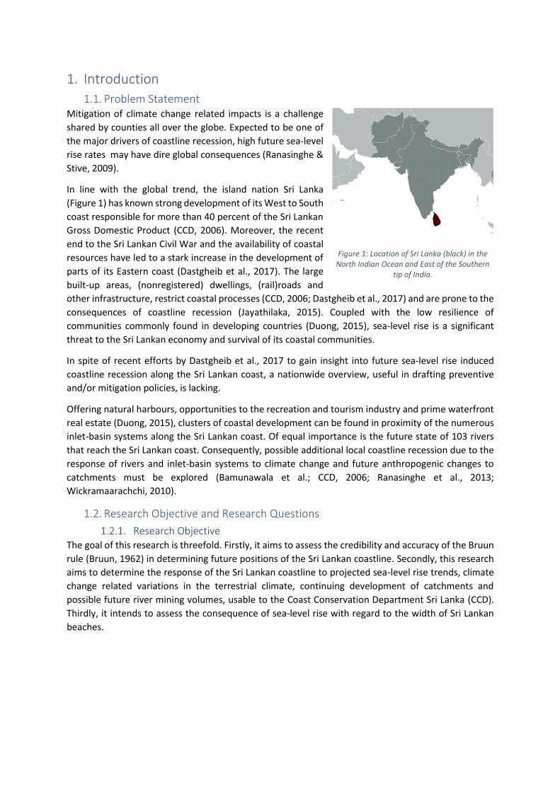
In line with the global trend, the island nation Sri Lanka
(Figure 1) has known strong development of its West to South
coast responsible for more than 40 percent of the Sri Lankan
Gross Domestic Product (CCD, 2006). Moreover, the recent
end to the Sri Lankan Civil War and the availability of coastal
resources have led to a stark increase in the development of
parts of its Eastern coast (Dastgheib et al., 2017). The large
built-up areas, (nonregistered) dwellings, (rail)roads and
other infrastructure, restrict coastal processes (CCD, 2006; Dastgheib et al., 2017) and are prone to the
consequences of coastline recession (Jayathilaka, 2015). Coupled with the low resilience of
communities commonly found in developing countries (Duong, 2015), sea-level rise is a significant
threat to the Sri Lankan economy and survival of its coastal communities.
In spite of recent efforts by Dastgheib et al., 2017 to gain insight into future sea-level rise induced
coastline recession along the Sri Lankan coast, a nationwide overview, useful in drafting preventive
and/or mitigation policies, is lacking.
Offering natural harbours, opportunities to the recreation and tourism industry and prime waterfront
real estate (Duong, 2015), clusters of coastal development can be found in proximity of the numerous
inlet-basin systems along the Sri Lankan coast. Of equal importance is the future state of 103 rivers
that reach the Sri Lankan coast. Consequently, possible additional local coastline recession due to the
response of rivers and inlet-basin systems to climate change and future anthropogenic changes to
catchments must be explored (Bamunawala et al.; CCD, 2006; Ranasinghe et al., 2013;
Wickramaarachchi, 2010).
1.2. Research Objective and Research Questions
1.2.1. Research Objective The goal of this research is threefold. Firstly, it aims to assess the credibility and accuracy of the Bruun
rule (Bruun, 1962) in determining future positions of the Sri Lankan coastline. Secondly, this research
aims to determine the response of the Sri Lankan coastline to projected sea-level rise trends, climate
change related variations in the terrestrial climate, continuing development of catchments and
possible future river mining volumes, usable to the Coast Conservation Department Sri Lanka (CCD).
Thirdly, it intends to assess the consequence of sea-level rise with regard to the width of Sri Lankan
beaches.
Figure 1: Location of Sri Lanka (black) in the North Indian Ocean and East of the Southern
tip of India.
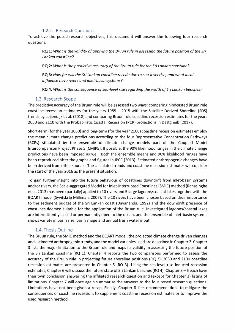
1.2.2. Research Questions To achieve the posed research objectives, this document will answer the following four research
questions.
RQ 1: What is the validity of applying the Bruun rule in assessing the future position of the Sri
Lankan coastline?
RQ 2: What is the predictive accuracy of the Bruun rule for the Sri Lankan coastline?
RQ 3: How far will the Sri Lankan coastline recede due to sea-level rise, and what local
influence have rivers and inlet-basin systems?
RQ 4: What is the consequence of sea-level rise regarding the width of Sri Lankan beaches?
1.3. Research Scope The predictive accuracy of the Bruun rule will be assessed two ways; comparing hindcasted Bruun rule
coastline recession estimates for the years 1985 – 2015 with the Satellite Derived Shoreline (SDS)
trends by Luijendijk et al. (2018) and comparing Bruun rule coastline recession estimates for the years
2050 and 2110 with the Probabilistic Coastal Recession (PCR) projections in Dastgheib (2017).
Short-term (for the year 2050) and long-term (for the year 2100) coastline recession estimates employ
the mean climate change predictions according to the four Representative Concentration Pathways
(RCPs) stipulated by the ensemble of climate change models part of the Coupled Model
Intercomparison Project Phase 5 (CMIP5). If possible, the 90% likelihood ranges in the climate change
predictions have been imposed as well. Both the ensemble means and 90% likelihood ranges have
been reproduced after the graphs and figures in IPCC (2013). Estimated anthropogenic changes have
been derived from other sources. The calculated trends and coastline recession estimates will consider
the start of the year 2016 as the present situation.
To gain further insight into the future behaviour of coastlines downdrift from inlet-basin systems
and/or rivers, the Scale-aggregated Model for Inlet-interrupted Coastlines (SMIC) method (Ranasinghe
et al. 2013) has been (partially) applied to 10 rivers and 5 large lagoons/coastal lakes together with the
BQART model (Syvitski & Milliman, 2007). The 10 rivers have been chosen based on their importance
to the sediment budget of the Sri Lankan coast (Dayananda, 1992) and the downdrift presence of
coastlines deemed suitable for the application of the Bruun rule. Investigated lagoons/coastal lakes
are intermittently closed or permanently open to the ocean, and the ensemble of inlet-basin systems
shows variety in basin size, basin shape and annual fresh water input.
1.4. Thesis Outline The Bruun rule, the SMIC method and the BQART model, the projected climate change driven changes
and estimated anthropogenic trends, and the model variables used are described in Chapter 2. Chapter
3 lists the major limitation to the Bruun rule and maps its validity in assessing the future position of
the Sri Lankan coastline (RQ 1). Chapter 4 reports the two comparisons performed to assess the
accuracy of the Bruun rule in projecting future shoreline positions (RQ 2). 2050 and 2100 coastline
recession estimates are presented in Chapter 5 (RQ 3). Using the sea-level rise induced recession
estimates, Chapter 6 will discuss the future state of Sri Lankan beaches (RQ 4). Chapter 3 – 6 each have
their own conclusion answering the affiliated research question and (except for Chapter 3) listing of
limitations. Chapter 7 will once again summarise the answers to the four posed research questions.
Limitations have not been given a recap. Finally, Chapter 8 lists recommendations to mitigate the
consequences of coastline recession, to supplement coastline recession estimates or to improve the
used research method.

Because of the spatial scope, the Sri Lankan coast has been subdivided into eight coastal sectors
(modified after Jacobsen et al. (1987)) (Figure 2 and Table 1). Figure 2 also displays most of the
spatial locations mentioned in this document.
Table 1: Start and finish of the coastal sectors of Sri Lanka (modified after Jacobsen et al. (1987)). X and Y coordinates are in decimal degrees and use the WSG84 geographic coordinate system.
Coastal sector X (decimal degrees) Y (decimal degrees)
Southern Start:
Finish:
Galle
Tangalle
80.218
80.802
6.023
6.022
South-eastern Start:
Finish:
Tangalle
Arugam Bay
80.802
81.840
6.022
6.839
Eastern Start:
Finish:
Arugam Bay
Trincomalee Bay
81.840
81.279
6.839
8.547
North-eastern Start:
Finish:
Trincomalee Bay
Point Pedro
81.279
80.256
8.547
9.817
Northern Start:
Finish:
Point Pedro
Vaddukoddai
80.256
79.931
9.817
9.779
North-western Start:
Finish:
Mannar Island
Kandakuliya
79.851
79.706
9.079
8.143
Western Start:
Finish:
Kandakuliya
Bentota
79.706
79.974
8.143
6.463
South-western Start:
Finish:
Bentota
Galle
79.974
80.218
6.463
6.023

Figure 2: Delineated coastal sectors of Sri Lanka (modified after Jacobsen et al. (1987)), location of investigated lagoons, coastal lakes and rivers, and spatial locations mentioned in the document (Baselayer: Google Earth).

2. Research Methodology Chapter 2 provides the necessary details on the delineation of defined coastal zones (Paragraph 2.2), the calculation methods
used (Paragraphs 2.3 – 2.5), future (and past) trends accounted for (Paragraphs 2.6 – 2.8) and the model variables used as
input (Paragraph2.9 – 2.11). Paragraph 2.1 outlines the use of each aforementioned paragraph in answering the posed
research questions.
2.1. Outline Research Methodology
Figure 3: Calculation methods, future (and past) trends, model variables and other data used to answer the posed research questions. Respective paragraph numbers are between brackets.

2.2. Defined Coastal Zones To estimate sea-level rise induced coastline recession,
the Sri Lankan coast has been subdivided into 211 zones
deemed suitable for the application of the Bruun rule
(indicated by one arrow each in Figure 6).
Because of the complex and significant divergences in
the littoral drift of coastal sediments, the Puttalam
sandspit (Figure 4) and the Vaddukoddai sandspit have
been excluded (Ranasinghe & Stive, 2009) together
with the coastline protected from the offshore wave
climate by the Puttalam sandspit. The ill-defined muddy
(Dayananda, 1992) coast between the Vaddukoddai
sandspit and Mannar Island has been omitted too.
Notorious for the offshore loss of coastal sediments to
the Trincomalee Canyon (CCD, 2006; Dayananda, 1992),
the otherwise suitable sandy coastline inside
Trincomalee Bay (Figure 5) has been precluded (after
Zhang et al. (2004)).
Lastly, rocky shorefaces, shorelines positioned behind
interrupted reefs (Figure 8), influenced by a series of
jetties or breakwaters, or protected by revetments
have been excluded. However, beaches between
breakwaters and jetties that may be assumed embayed
Figure 5: Omitted coastline (yellow dotted arrows) inside Trincomalee Bay (Baselayer: Google Earth).
Figure 4: Defined coastal zones (yellow continuous arrows) at the Puttalam sandspit (Baselayer: Google
Earth).
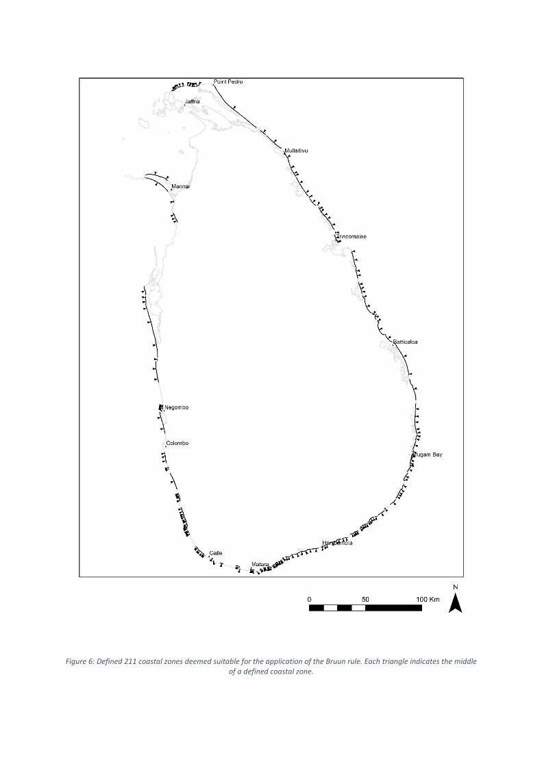
Figure 6: Defined 211 coastal zones deemed suitable for the application of the Bruun rule. Each triangle indicates the middle of a defined coastal zone.

Figure 7: Sandy coastline behind continuous reefs West of
the Thondamannaru Lagoon inlet (Google Earth).
Figure 8: Sandy coastline influenced by the construction of a series of small jetties and positioned behind interrupted
reefs at Point Pedro (Google Earth).
Figure 9: Defined coastal zones (yellow continuous arrows) between breakwaters and jetties South of the Kalu Ganga
river mouth (Baselayer: Google Earth).
Figure 10: The sediment poor and heavily engineered
coastline South of the Gin Ganga river mouth and sandspit (Baselayer: Google Earth).
beaches with a closed circulation of coastal sediments (e.g. the beaches South of the Kalu Ganga river mouth (Figure 9) and North of the Negombo Lagoon inlet) have been included. Defined coastal zones have been delineated using headlands, jetties, breakwaters, river mouths, inlets of intermittently closed to permanently open inlet-basin systems, known nodal points in the littoral drift of coastal sediments as their borders. At all times, a safe distance to river mouths and inlets was maintained.

2.3. The Bruun Rule Important to many studies regarding the future position of coastlines is the Bruun principle. First
described by Bruun (1962), the Bruun principle assumes the persistence of an equilibrium shaped
active shoreface, forcing it to move upwards with rising sea-levels. Sediments required to lift the active
shoreface are provided through the redistribution of coastal sediments, resulting in a landward
migration by the active shoreface. Zhang et al. (2004) attribute the redistribution of shoreface
sediments to heavy weather waves. Understandably, the landwards height limit (DB [m]) and the
seawards depth limit (DC [m]) to the active shoreface are dependent upon their ability to work the
coastal sediments.
Provided the assumption regarding the persistence of the equilibrium shaped active shoreface holds,
Zhang et al. (2004) explain that sea-level rise induced coastline recession (RBE [m]) can be linked to sea-
level rise using, in current literature often referred to as, the Bruun rule.
𝑅𝐵𝐸 =𝐿∗
𝐷𝐵 + 𝐷𝐶𝛥𝑅𝑆𝐿 (1)
With ΔRSL [m] the regional relative increase in sea-level, L* [m] the cross-shore distance between the
positions of the landward and seawards limits to the active shoreface (Figure 11).
Figure 11: Sea-level rise induced coastline recession according to the Bruun rule for an equilibrium shaped active shoreface f. Modified after Zhang et al (2004).

2.3.1. The Landward Limit to The Active Shoreface Instead of Equation 1, this research will employ the first proposed wording of the Bruun rule by Bruun
(1962).
𝑅𝐵𝐸 =𝐿∗
𝐷𝐶𝛥𝑅𝑆𝐿 (2)
With L* the cross-shore distance between the mean sea-level (MSL) mark and the seaward limit to the
active shoreface. The diversion from Equation 1 has multiple reasons.
▪ DB can be estimated by combining Sunamura (1975), Sunamura (1983), and Takeda and
Sunamura (1983). However, the use of non site-specifically calibrated predictors for the beach
slope (Velegrakis & Schimmels, 2013) results in an overestimation of surveyed berm heights.
The alternative, employing bathymetric and topographic surveys to determine DB accurately,
is a tedious and ambiguous process often hindered by the resolution of available surveys.
▪ As per the derivation of Dean’s equilibrium profile (Dean & Dalrymple, 2001):
ℎ = 𝐴𝐸𝑃(𝑑50) 𝑥2
3⁄ (3)
with the shape factor AEP [m1/3] determined through the mean grain size (d50), the use of
Equation 4 is restricted to the shoreface seaward from the MSL mark.
▪ The persistence of the equilibrium shaped shoreface above MSL is a questionable extension of
the assumptions originally part of the Bruun rule. Wet sediments below MSL are more mobile
than the dry sediments that (partially) make up the berm. Therefore, the landward migration
of the berm is expected to lag that of the MSL mark.
▪ For high quality cross-shore profiles along the East coast of Sri Lanka, the use of Equation 1 will
result in 14% smaller and therefore less conservative coastline recession estimates.
2.3.2. The Seaward Limit to The Active Shoreface Regarding the depth of closure, Nicholls et al.’s (1996) estimate:
𝐷𝐶 = 2.28 𝐻𝑒,𝑡 − 68.5 (𝐻𝑒,𝑡
2
𝑔 𝑇𝑒,𝑡2) (4)
with g [m s-2] the gravitational acceleration, He,t [m] the non-breaking significant wave height that is
exceeded 12 hours within a timescale of t years and Te,t [s] the associated wave period, is one of the
more often applied estimates for DC (Ranasinghe & Stive, 2009).
To determine the offshore location of the seaward limit to the active shoreface, the shape of the
equilibrium profile is needed. Since the depth of closure is defined as the depth at which no significant
change in the profile is observed (Nicholls et al., 1996), present cross-shore profiles are believed useful
in providing site-specific values for L*.
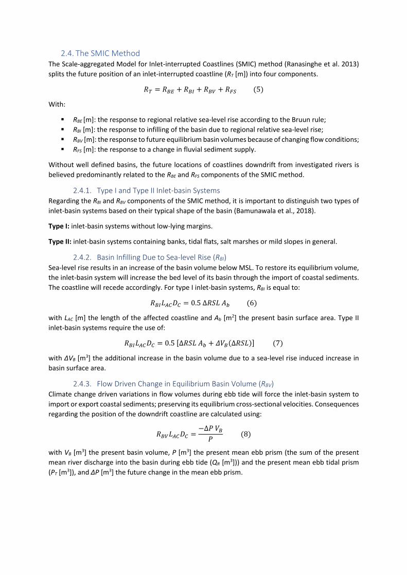
2.4. The SMIC Method The Scale-aggregated Model for Inlet-interrupted Coastlines (SMIC) method (Ranasinghe et al. 2013)
splits the future position of an inlet-interrupted coastline (RT [m]) into four components.
𝑅𝑇 = 𝑅𝐵𝐸 + 𝑅𝐵𝐼 + 𝑅𝐵𝑉 + 𝑅𝐹𝑆 (5)
With:
▪ RBE [m]: the response to regional relative sea-level rise according to the Bruun rule;
▪ RBI [m]: the response to infilling of the basin due to regional relative sea-level rise;
▪ RBV [m]: the response to future equilibrium basin volumes because of changing flow conditions;
▪ RFS [m]: the response to a change in fluvial sediment supply.
Without well defined basins, the future locations of coastlines downdrift from investigated rivers is
believed predominantly related to the RBE and RFS components of the SMIC method.
2.4.1. Type I and Type II Inlet-basin Systems Regarding the RBI and RBV components of the SMIC method, it is important to distinguish two types of
inlet-basin systems based on their typical shape of the basin (Bamunawala et al., 2018).
Type I: inlet-basin systems without low-lying margins.
Type II: inlet-basin systems containing banks, tidal flats, salt marshes or mild slopes in general.
2.4.2. Basin Infilling Due to Sea-level Rise (RBI) Sea-level rise results in an increase of the basin volume below MSL. To restore its equilibrium volume,
the inlet-basin system will increase the bed level of its basin through the import of coastal sediments.
The coastline will recede accordingly. For type I inlet-basin systems, RBI is equal to:
𝑅𝐵𝐼𝐿𝐴𝐶𝐷𝐶 = 0.5 ∆𝑅𝑆𝐿 𝐴𝑏 (6)
with LAC [m] the length of the affected coastline and Ab [m2] the present basin surface area. Type II
inlet-basin systems require the use of:
𝑅𝐵𝐼𝐿𝐴𝐶𝐷𝐶 = 0.5 [∆𝑅𝑆𝐿 𝐴𝑏 + 𝛥𝑉𝐵(∆𝑅𝑆𝐿)] (7)
with ΔVB [m3] the additional increase in the basin volume due to a sea-level rise induced increase in
basin surface area.
2.4.3. Flow Driven Change in Equilibrium Basin Volume (RBV) Climate change driven variations in flow volumes during ebb tide will force the inlet-basin system to
import or export coastal sediments; preserving its equilibrium cross-sectional velocities. Consequences
regarding the position of the downdrift coastline are calculated using:
𝑅𝐵𝑉𝐿𝐴𝐶𝐷𝐶 =−∆𝑃 𝑉𝐵
𝑃 (8)
with VB [m3] the present basin volume, P [m3] the present mean ebb prism (the sum of the present
mean river discharge into the basin during ebb tide (QR [m3])) and the present mean ebb tidal prism
(PT [m3]), and ΔP [m3] the future change in the mean ebb prism.
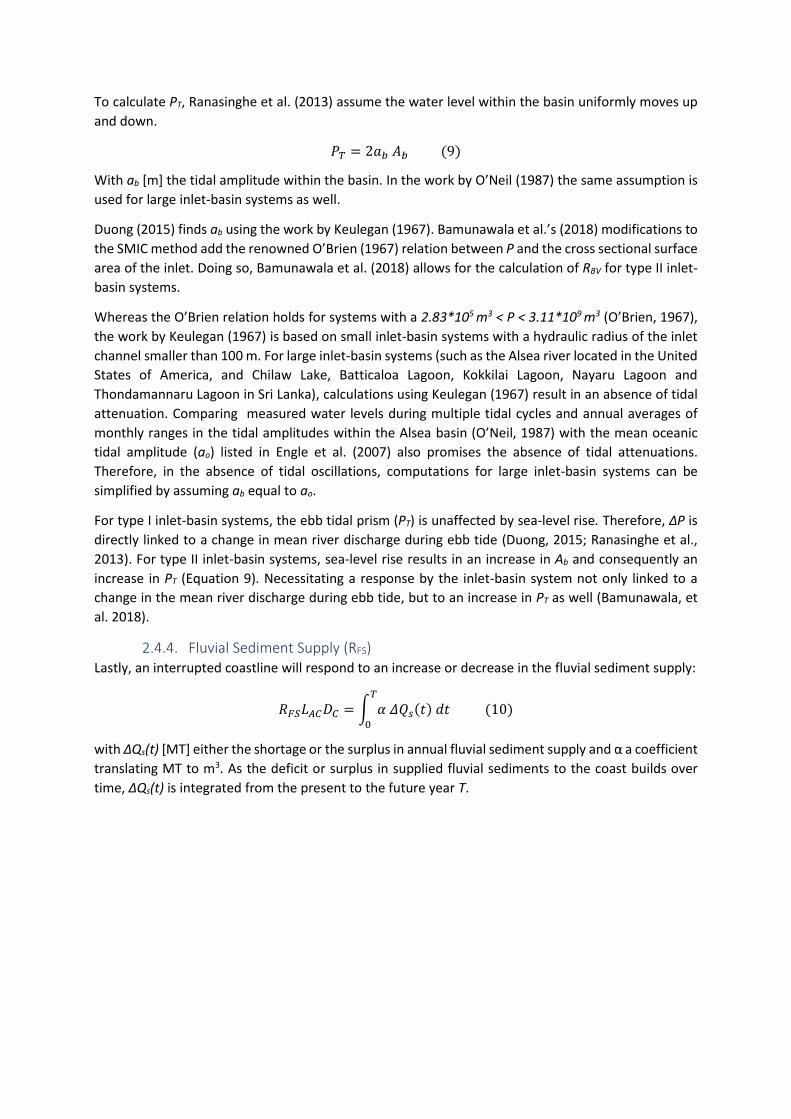
To calculate PT, Ranasinghe et al. (2013) assume the water level within the basin uniformly moves up
and down.
𝑃𝑇 = 2𝑎𝑏 𝐴𝑏 (9)
With ab [m] the tidal amplitude within the basin. In the work by O’Neil (1987) the same assumption is
used for large inlet-basin systems as well.
Duong (2015) finds ab using the work by Keulegan (1967). Bamunawala et al.’s (2018) modifications to
the SMIC method add the renowned O’Brien (1967) relation between P and the cross sectional surface
area of the inlet. Doing so, Bamunawala et al. (2018) allows for the calculation of RBV for type II inlet-
basin systems.
Whereas the O’Brien relation holds for systems with a 2.83*105 m3 < P < 3.11*109 m3 (O’Brien, 1967),
the work by Keulegan (1967) is based on small inlet-basin systems with a hydraulic radius of the inlet
channel smaller than 100 m. For large inlet-basin systems (such as the Alsea river located in the United
States of America, and Chilaw Lake, Batticaloa Lagoon, Kokkilai Lagoon, Nayaru Lagoon and
Thondamannaru Lagoon in Sri Lanka), calculations using Keulegan (1967) result in an absence of tidal
attenuation. Comparing measured water levels during multiple tidal cycles and annual averages of
monthly ranges in the tidal amplitudes within the Alsea basin (O’Neil, 1987) with the mean oceanic
tidal amplitude (ao) listed in Engle et al. (2007) also promises the absence of tidal attenuations.
Therefore, in the absence of tidal oscillations, computations for large inlet-basin systems can be
simplified by assuming ab equal to ao.
For type I inlet-basin systems, the ebb tidal prism (PT) is unaffected by sea-level rise. Therefore, ΔP is
directly linked to a change in mean river discharge during ebb tide (Duong, 2015; Ranasinghe et al.,
2013). For type II inlet-basin systems, sea-level rise results in an increase in Ab and consequently an
increase in PT (Equation 9). Necessitating a response by the inlet-basin system not only linked to a
change in the mean river discharge during ebb tide, but to an increase in PT as well (Bamunawala, et
al. 2018).
2.4.4. Fluvial Sediment Supply (RFS) Lastly, an interrupted coastline will respond to an increase or decrease in the fluvial sediment supply:
𝑅𝐹𝑆𝐿𝐴𝐶𝐷𝐶 = ∫ 𝛼 𝛥𝑄𝑠(𝑡) 𝑑𝑡𝑇
0
(10)
with ΔQs(t) [MT] either the shortage or the surplus in annual fluvial sediment supply and α a coefficient
translating MT to m3. As the deficit or surplus in supplied fluvial sediments to the coast builds over
time, ΔQs(t) is integrated from the present to the future year T.

2.5. The BQART Model The annual fluvial sediment supply can be approximated using the BQART model proposed by Syvitski
et al. (2007). With the annual mean temperature in Sri Lanka above 2°C and the absence of ice cover,
the annual fluvial sediment supply of a river is approximately:
𝑄𝑠 = 𝜔𝐵𝑄0.31𝐴0.5𝑅𝑇 (11)
with ω = 0.0006, A [km2] the catchment area, R [km] the highest point of elevation above MSL inside
the catchment, T [°C] the catchment-wide annual mean temperature, and B as in:
𝐵 = 𝐿(1 − 𝑇𝐸)𝐸ℎ (12)
with L the catchment-wide lithology factor (L = 0.5 (Syvitski & Milliman, 2007)), TE the catchment-wide
sediment trapping efficiency by reservoirs and Eh the catchment-wide anthropogenic factor reflecting
the human influence on soil erosion processes.
2.5.1. Trapping Efficiency (TE) According to Verstraeten and Poesen (2000), empirical models are well suited to determine the annual
trapping efficiency of a reservoir (TEres). The applicability of the median reservoir trapping efficiency
curve proposed by Brune (1953) is limited to large reservoirs (Vres > 500 Mm3). Small reservoirs (Vres ≤
500 Mm3) require the modified median Brune curve by Heinemann (1981). The catchment-wide
trapping efficiency (TE) is determined using Vörösmarty et al. (2003):
𝑇𝐸 =∑ (𝑇𝐸𝑏𝑎𝑠,𝑘 𝑄𝑏𝑎𝑠,𝑘)𝑚
𝑘=1
𝑄 (13)
with Qbas the annual discharge of the sub-catchment regulated by reservoir k, m the number of
controlled sub-catchments draining parallel to one another inside the catchment and Q the annual
river discharge. Provided there are no nested reservoirs, TEbas,k is equal to TEres. However, for any
reservoir with one or more nested reservoirs, the method proposed by Kummu et al. (2010) should be
used.
𝑇𝐸𝑏𝑎𝑠,𝑗 = 1 − (1 − 𝑇𝐸𝑟𝑒𝑠,𝑗) 𝑄𝑏𝑎𝑠,𝑗 − ∑ (𝑄𝑏𝑎𝑠,𝑗−1,𝑘 𝑇𝐸𝑏𝑎𝑠,𝑗−1,𝑘)𝑚
𝑘=1
𝑄𝑏𝑎𝑠,𝑗 (14)
With m the number of sub-catchments regulated by reservoirs found directly upstream (j-1) from the
controlling reservoir j.
Future TEres values are decreased by increasing freshwater inputs and reservoir siltation (Verstraeten
& Poesen 2000). The latter has been approximated using two BQART model runs; with reservoirs and
without reservoirs. The difference between the two is believed the annual catchment-wide volume of
reservoir siltation that can be subdivided over the individual reservoirs in the catchment.
2.5.2. River Mining Activities (Vm) Annual river mining activities (Vm) can be subtracted from the BQART model results (Bamunawala et
al., 2018). However, reservoir trapping efficiency calculations show large (TEres > 0.9) present and
future efficiencies. River mining activities upstream from these reservoirs hardly impact present and
future fluvial sediment supplies. Consequently, subtracting Vm from the BQART model results for rivers
with large downstream reservoirs and high catchment-wide trapping efficiencies would result in a too
large decreases in QS. Without a sound approach to include river mining activities in Equation 13 and
Equation 14, possible river mining activities in said rivers have been ignored.
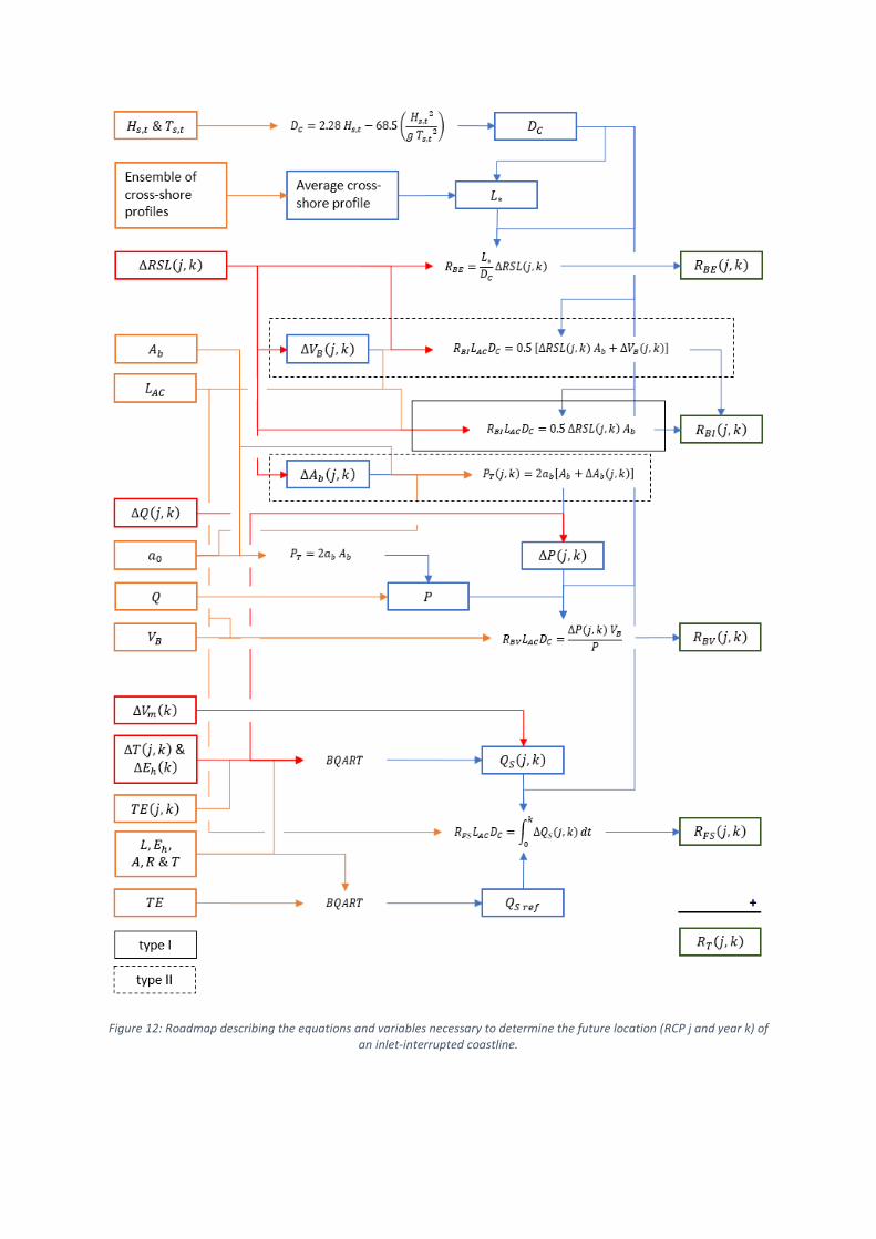
Figure 12: Roadmap describing the equations and variables necessary to determine the future location (RCP j and year k) of an inlet-interrupted coastline.
2.6. Climate Change Related Rise in Sea-level
2.6.1. Future Regional Relative Sea-level Rise (ΔRSL) Without large uninterrupted research quality data records (30 – 35 years or more) describing past
regional relative sea-level rise trends along the Sri Lankan coast, model-based projections must be
used (Nicholls et al., 2014). Nicholls et al. (2014) break down regional relative sea-level rise into:
∆𝑅𝑆𝐿 = ∆𝑆𝐿𝐺 + ∆𝑆𝐿𝑅𝑀 + ∆𝑆𝐿𝑅𝐺 + ∆𝑆𝐿𝑅𝐿𝑀 (15)
with ΔSLG [m] the global change in sea-level, ΔSLRM [m] the regional meteo-oceanic factors (wind fields
and related distribution of heat and freshwater, and atmospheric loading), ΔSLRG [m] the regional
gravity field changes (linked to the cryosphere and terrestrial water storage), and ΔSLRLM [m] the
regional vertical land movements (glacio-isostatic adjustment, tectonic movements and anthropogenic
land subsidence rates) (Ballu et al., 2011; IPCC, 2013; Nicholls et al., 2014).
To build the mean, and 95% and 5% likelihood 2100 time series for all four RCPs used in the Bruun rule
coastline recession estimates, the approach described in Dastgheib et al. (2017) has been employed.
Information regarding the global (ΔSLG) and regional (ΔSLRM, SLRG and SLRLM) components in Equation
15 originate from Argus et al. (2014), Peltier et al. (2015) and IPCC (2013).
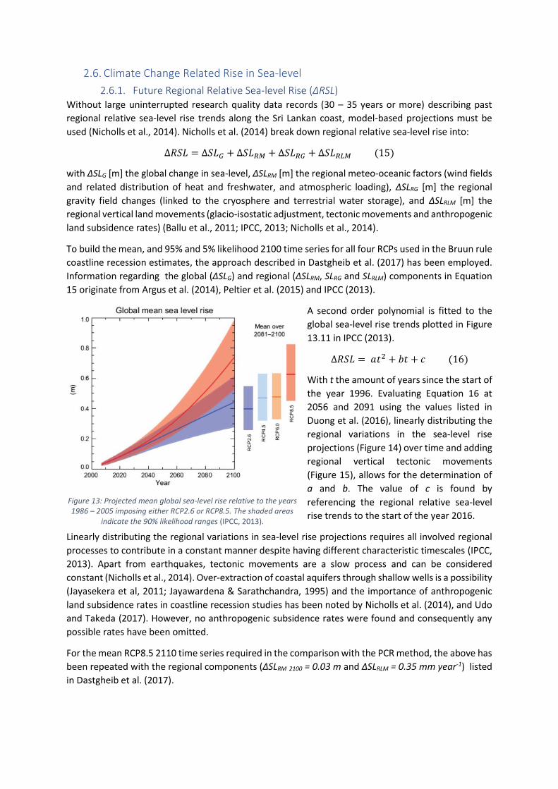
A second order polynomial is fitted to the
global sea-level rise trends plotted in Figure
13.11 in IPCC (2013).
∆𝑅𝑆𝐿 = 𝑎𝑡2 + 𝑏𝑡 + 𝑐 (16)
With t the amount of years since the start of
the year 1996. Evaluating Equation 16 at
2056 and 2091 using the values listed in
Duong et al. (2016), linearly distributing the
regional variations in the sea-level rise
projections (Figure 14) over time and adding
regional vertical tectonic movements
(Figure 15), allows for the determination of
a and b. The value of c is found by
referencing the regional relative sea-level
rise trends to the start of the year 2016.
Linearly distributing the regional variations in sea-level rise projections requires all involved regional
processes to contribute in a constant manner despite having different characteristic timescales (IPCC,
2013). Apart from earthquakes, tectonic movements are a slow process and can be considered
constant (Nicholls et al., 2014). Over-extraction of coastal aquifers through shallow wells is a possibility
(Jayasekera et al, 2011; Jayawardena & Sarathchandra, 1995) and the importance of anthropogenic
land subsidence rates in coastline recession studies has been noted by Nicholls et al. (2014), and Udo
and Takeda (2017). However, no anthropogenic subsidence rates were found and consequently any
possible rates have been omitted.
For the mean RCP8.5 2110 time series required in the comparison with the PCR method, the above has
been repeated with the regional components (ΔSLRM 2100 = 0.03 m and ΔSLRLM = 0.35 mm year-1) listed
in Dastgheib et al. (2017).
Figure 13: Projected mean global sea-level rise relative to the years 1986 – 2005 imposing either RCP2.6 or RCP8.5. The shaded areas
indicate the 90% likelihood ranges (IPCC, 2013).

Figure 14:Regional variations [mm] in the mean sea-level rise projections by IPCC (2013) for the years 2081 – 2100. Values have been acquired by subtracting the global mean sea-level rise trends listed in Duong et al. (2016) from the regional mean
sea-level rise trends made available in netCDF format by the Integrated Climate Data Center (ICDC, icdc.cen.uni-hamburg.de) University of Hamburg, Hamburg, Germany.
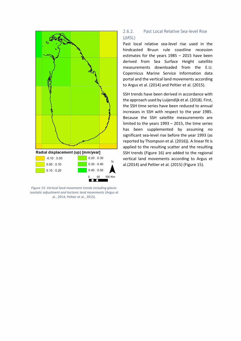
2.6.2. Past Local Relative Sea-level Rise
(ΔRSL) Past local relative sea-level rise used in the
hindcasted Bruun rule coastline recession
estimates for the years 1985 – 2015 have been
derived from Sea Surface Height satellite
measurements downloaded from the E.U.
Copernicus Marine Service Information data
portal and the vertical land movements according
to Argus et al. (2014) and Peltier et al. (2015).
SSH trends have been derived in accordance with
the approach used by Luijendijk et al. (2018). First,
the SSH time series have been reduced to annual
increases in SSH with respect to the year 1985.
Because the SSH satellite measurements are
limited to the years 1993 – 2015, the time series
has been supplemented by assuming no
significant sea-level rise before the year 1993 (as
reported by Thompson et al. (2016)). A linear fit is
applied to the resulting scatter and the resulting
SSH trends (Figure 16) are added to the regional
vertical land movements according to Argus et
al.(2014) and Peltier et al. (2015) (Figure 15).
Figure 15: Vertical land movement trends including glacio-isostatic adjustment and tectonic land movements (Argus et
al., 2014; Peltier et al., 2015).

Figure 16: 1985 – 2015 Sea Surface Height (SSH) trends calculated using E.U. Copernicus Marine Service Information. Black solid lines indicate hindcasted defined coastal zones and nourishment schemes completed between the years 1985 – 2015
have been marked using circles (with structures) and squares (without structures).

2.7. Future Climate Change Driven Variations in The Terrestrial Climate
2.7.1. Variations in Annual Mean Temperatures (ΔT) Because of the size, shape and offshore position of Sri Lanka, the Sri Lankan climate is moderated by
its the surrounding waters (Department of Meteorology Sri Lanka, 2016). Therefore, increments in the
annual mean temperature have been derived from the projections for the North Indian Ocean in Figure
17 (Figure AI.60 and Figure AI.61 in IPCC (2013)).
The mean (solid lines in Figure 17) annual rate at which T is expected to increase is 0.0036 °C year-1
(RCP2.6), 0.014 °C year-1 (RCP4.5), 0.020 °C year-1 (RCP6.0) or 0.038 °C year-1 (RCP8.5). 5% and 95%
likelihood bands have been derived from the the two boxplot graphs in Figure 17.
Figure 17: Hindcasted and forecasted mean surface temperature change during the months December – February (left frame) and June – August (right frame) for the North Indian Ocean (solid lines). Boxplot graphs summarising the 2081 – 2100 results of the CMIP5 models are plotted to the right of each frame (Figure AI.60 and Figure AI.61 in IPCC (2013)).
2.7.2. Increases in Annual River Discharges (ΔQ) Future increases in annual river discharges have been estimated using the annual mean runoff change
projections in Figure 12.24 in IPCC (2013). The projected changes in daily runoff have been transformed
into changes in annual runoff and divided by the amount of years until the end of the 21st century to
find the yearly increments of 0.246 mm year-1 (RCP2.6 and RCP4.5), 0.740 mm year-1 (RCP6.0) or 1.23
mm year-1 (RCP8.5). Increases in annual river discharges have been ascertained by multiplying the
yearly increment in annual runoff with the catchment areas of investigated rivers.
2.8. Future Anthropogenic Changes to The Catchments
2.8.1. Continuing Development of The River Catchments (ΔEh) Land clearance and other future human alterations are believed to increasingly affect soil erosion
processes in river catchments. Within the Kalu Ganga catchment several large development projects
are planned and a 20% increase in Eh is expected by Bamunawala et al. (2018). Without an alternative,
the estimate mentioned in Bamunawala et al. (2018) has been used to describe the middle increase in
the catchment-wide anthropogenic factor with respect to the present value (0.24% year-1). Crude
lower likelihood (0.12% year-1) and upper likelihood (0.30% year-1) bands have been added.
2.8.2. Increases in River Mining Activities (ΔVm) Rapidly increasing since early 2000 and linked to economic growth (Jayathilaka, 2015), river mining
activities are expected to continue to increase. Bamunawala et al. (2018) estimate a 25% growth in
river mining activities before the end of the 21st century. Assuming a linear relationship, said estimate
results in a 0.30% year-1 increase in possible river mining activities with respect to the present situation.
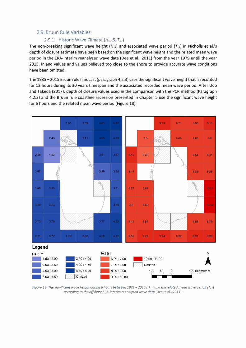
2.9. Bruun Rule Variables
2.9.1. Historic Wave Climate (Hs,t & Ts,t) The non-breaking significant wave height (Hs,t) and associated wave period (Ts,t) in Nicholls et al.’s
depth of closure estimate have been based on the significant wave height and the related mean wave
period in the ERA-Interim reanalysed wave data (Dee et al., 2011) from the year 1979 untill the year
2015. Inland values and values believed too close to the shore to provide accurate wave conditions
have been omitted.
The 1985 – 2015 Bruun rule hindcast (paragraph 4.2.3) uses the significant wave height that is recorded
for 12 hours during its 30 years timespan and the associated recorded mean wave period. After Udo
and Takeda (2017), depth of closure values used in the comparison with the PCR method (Paragraph
4.2.3) and the Bruun rule coastline recession presented in Chapter 5 use the significant wave height
for 6 hours and the related mean wave period (Figure 18).
Figure 18: The significant wave height during 6 hours between 1979 – 2015 (He,t) and the related mean wave period (Te,t) according to the offshore ERA-Interim reanalysed wave data (Dee et al., 2011).
2.9.2. Active Shoreface Dimensions (L*)
2.9.2.1. Acquisition of Cross-shore Profile Measurements
Cross-shore profiles have been extracted from bathymetry maps and xyz datafiles from the CCD, and
supplemented with a small collection of transects from CDR-International. The measurements have
been assumed perpendicular to the coast and clear artefacts (e.g. loops in the measurements, turns at
the beginning and/or end of transects and double takes) have either been solved manually or resulted
in the omission of an entire transect. To avoid the use of unfit transects (e.g. the nearshore shape is
influenced by revetments, breakwaters or headlands) only bathymetry measurements that line up with
defined coastal zones have been included. An exception was made for measurements near Jaffna,
Koggala and Hambantota. The sheer scarcity of measurements in these areas necessitated the use of
measurements outside defined coastal zones. The measurements at Hambantota predate the second
construction phase of the harbour.
At Mannar Island, Jaffna and Mullaitivu, cross-shore profile measurements were incomplete. The
missing depths between MSL and -2 to -3 m + MSL have been determined using Dean’s equilibrium
profile, the average median grain sizes listed in IHE-Delft (2016) and the look-up table for the
shapefactor in Dean and Dalrymple (2001). Shape factors for Mannar Island, Jaffna and Mullaitivu are
0.1482 (d50 = 420 μm), 0.1410 (d50 = 380 μm) and 0.1578 (d50 = 480 μm). Obvious mismatches between
Dean’s equilibrium profile and bathymetry measurements have been linked to cross-shore profile
measurements missing the entire final approach of MSL and respective transects have been omitted.
Remaining mismatches are believed to be solved by taking the average cross-shore profile of multiple
transects.
2.9.2.2. Cross-shore Profile Measurements Allocation
The positions of the resulting 273 suitable cross-shore profiles is depicted in Figure 20. Roughly half
the defined coastal zones has one or more cross-shore profiles within their longshore limits. All other
zones have been assigned representative cross-shore profiles (Figure 20).
Between Galle and Tangalle (~60 km gap), the cross-shore profiles at Unawatuna and Kogalla have
been assigned to respectively sheltered and exposed beaches. Between Tangalle and Oluvil (~160 km
gap), bathymetry measurements at Tangalle and Hambantota have been used to draw approximate
cross-shore profiles for sheltered and exposed beaches, and a combination of the two. Closer to Oluvil,
the cross-shore profile at Oluvil has been used as well. To the North of Chilaw (~70 km gap), the
bathymetry measurements along the Chilaw – Negombo coastline have been reused.
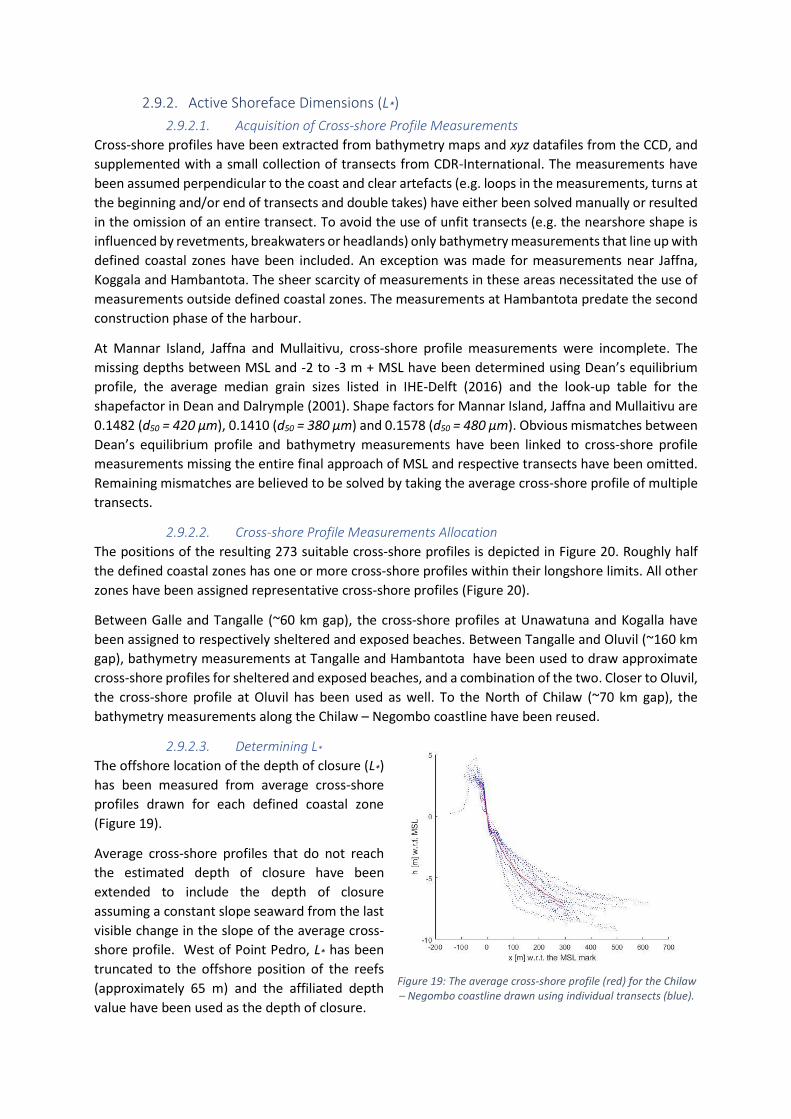
2.9.2.3. Determining L*
The offshore location of the depth of closure (L*)
has been measured from average cross-shore
profiles drawn for each defined coastal zone
(Figure 19).
Average cross-shore profiles that do not reach
the estimated depth of closure have been
extended to include the depth of closure
assuming a constant slope seaward from the last
visible change in the slope of the average cross-
shore profile. West of Point Pedro, L* has been
truncated to the offshore position of the reefs
(approximately 65 m) and the affiliated depth
value have been used as the depth of closure.
Figure 19: The average cross-shore profile (red) for the Chilaw – Negombo coastline drawn using individual transects (blue).

Figure 20: Use and location of suitable transects. Cross-shore measurements that required supplements provided by Dean’s equilibrium profile have been marked with an ‘x’.

2.10. SMIC Method Variables
Table 2: Present SMIC method model variables: length of affected coastline (LAC), annual river discharge (Q), mean oceanic tidal amplitude (ao), basin surface area (Ab) and basin volume (VB).
LAC [m] Q [Mm3] ao [m] Ab [km2] VB [Mm3]
Type I lagoons/Coastal lakes
Chilaw lake
Batticaloa Lagoon
Kokkilai Lagoon
20000
10400
11400
-
1460
358
0.33
0.26
0.39
5.3
83.2
47.6
18.6
291
71.4
Type II lagoons
Nayaru Lagoon
Thondamannaru Lagoon
20000
5500
87
-
0.41
0.43
7.1
8.9
9.94
22.3
Rivers
Deduru Oya
Kelani Ganga
Kalu Ganga
Gin Ganga
Nilwala Ganga
Walawe Ganga
Kirindi Oya
Menik Ganga
Kumbukkan Oya
Gal Oya
20000
-
-
-
1200
-
3400
7800
3100
20000
1180
5570
7600
1970
1410
1680
305
215
250
148
2.10.1. Present Mean River Discharges During Ebb Tide (QR) Annual discharges by the tributaries of Batticaloa Lagoon, Kokkilai Lagoon and Nayaru Lagoon have
been reproduced after those listed in Silva et al. (2013). Without tributaries, Thondamannaru Lagoon
is believed to receive no annual freshwater input. Likewise, with the Deduru Oya river bypassing Chilaw
Lake, the latter will experience a negligible annual freshwater input.
Concerning the annual river discharges, the values by the Survey Department of Sri Lanka (1983) have
been used. For eight out of the ten rivers, recent discharge measurements for one year have been
acquired by the CCD. However, concerns about their accuracy regarding the interannual mean could
not be addressed. Moreover, in combination with Table 5, the use of said discharge measurements for
heavily controlled catchments does not result in catchment-wide trapping efficiencies conform the
condition (0 ≤ TE < 0.9) set by Syvitski et al. (2016).
2.10.2. Mean Oceanic Tidal Amplitudes (ao) Although the M2 tidal constituent explains most of the tidal range in the waters surrounding Sri Lanka,
the tide is considered mixed semi-diurnal (Wijeratne & Pattiaratchi, 2017). Using the amplitude and
phase maps for the tidal constituents M2, S2, N2, K1 and O1, and the amplifications by the coastal
shelf in Sindhu and Unnikrishnan (2013), columns two and three in Table 3 have been determined.
Values for Chilaw Lake after from Wijeratne (n.d.). The individual tidal constituents have been added
using:
𝑎(𝑡) = ∑ 𝑎𝑛 𝑐𝑜𝑠(𝜎𝑛𝑡 − 𝜗𝑛) (17)
with a(t) the tidal amplitude at a moment t in time, and an the amplitude, σn the period and θn the
phase of tidal constituent n. Since M2 is the main tidal constituent, the tidal period of M2 has been

employed to find the compounded tidal amplitudes and mean oceanic tidal amplitude for one
simulated year.
Table 3: Tidal constituents according to Sindhu and Unnikrishnan (2013) and Wijeratne (n.d.), and resulting mean oceanic tidal amplitude (a0) at Chilaw Lake, Batticaloa Lagoon, Nayaru Lagoon, Kokkilai Lagoon and Thondamannaru Lagoon.
Constituent Amplitude (𝒂𝒏) [m] Phase w.r.t M2 (𝝑𝒏 ) [°] (a0) [m]
Chilaw Lake
M2 0.36 -
0.33 S2 0.22 47
K1 0.18 -2
O1 0.06 13
Batticaloa Lagoon
M2 0.225 -
0.26
S2 0.10 20
N2 0.055 -10
K1 0.04 190
O1 0.02 180
Kokkilai Lagoon
M2 0.35 -
0.39
S2 0.12 20
N2 0.08 -10
K1 0.04 190
O1 0.02 185
Nayaru Lagoon
M2 0.375 -
0.41
S2 0.125 20
N2 0.08 -10
K1 0.045 190
O1 0.02 185
Thondamannaru Lagoon
M2 0.40 -
0.43
S2 0.10 25
N2 0.09 -5
K1 0.045 190
O1 0.02 185
2.10.3. Present (Ab, VB) and Future Basin Surface Areas and Basin Volumes (ΔAb, ΔVB) Present basin surface areas have been measured from satellite images. For type II inlet basin systems,
the basin surface area varies with each satellite image taken. Here, the satellite image showing roughly
the average amount of basin surface area has been used. Present basin volumes have been acquired
by multiplying Ab with the average depths (3.5 m, 1.5 m, 1.4m, 2.5 m) estimated from bathymetry
maps regarding Chilaw Lake and Batticaloa Lagoon, Kokkilai Lagoon, Nayaru Lagoon, and
Thondamannaru Lagoon (Personal communication Silva, 2018).
Because of the negligible (fluctuations in) salinity levels in the Southernmost part of the Batticaloa
Lagoon basin (Silva et al., 2013) and since this sub-basin is connected to the remainder of Batticaloa
lagoon via a narrow channel, the Southernmost part of Batticaloa Lagoon is not believed to move with
the oceanic tide. However, It does receive a freshwater input. According to O’Neil (1987), and Stive
and Rakhorst (2008), the mean freshwater input during ebb tide is small compared to the mean ebb
tidal prism. Therefore, Ab and VB have been based on the Northern parts of Batticaloa Lagoon.
Thondamannaru Lagoon is a similar large system of which only the Western part is connected to the
ocean.
Due to its vertical accuracy (Wickramagamage et al., 2012), the NASA Shuttle Radar Topography
Mission (SRTM) Digital Elevation Model (Jarvis et al., 2008) cannot be used to determine ΔAb and ΔVB.
Instead, the tidal flats within Nayaru Lagoon and Thondamannaru Lagoon are assumed to have a
constant slope up to a height of 1 m + MSL at the landward edge of the tidal flat.
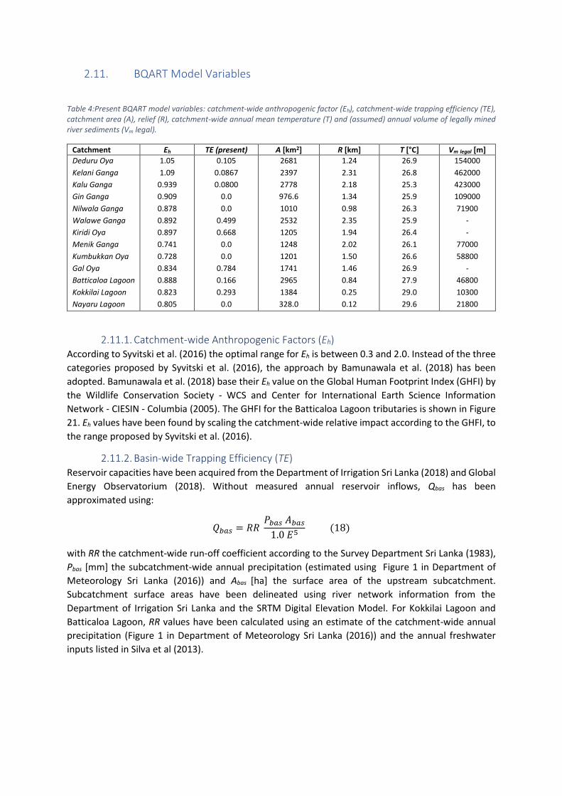
2.11. BQART Model Variables
Table 4:Present BQART model variables: catchment-wide anthropogenic factor (Eh), catchment-wide trapping efficiency (TE), catchment area (A), relief (R), catchment-wide annual mean temperature (T) and (assumed) annual volume of legally mined river sediments (Vm legal).
Catchment Eh TE (present) A [km2] R [km] T [°C] Vm legal [m]
Deduru Oya
Kelani Ganga
Kalu Ganga
Gin Ganga
Nilwala Ganga
Walawe Ganga
Kiridi Oya
Menik Ganga
Kumbukkan Oya
Gal Oya
Batticaloa Lagoon
Kokkilai Lagoon
Nayaru Lagoon
1.05
1.09
0.939
0.909
0.878
0.892
0.897
0.741
0.728
0.834
0.888
0.823
0.805
0.105
0.0867
0.0800
0.0
0.0
0.499
0.668
0.0
0.0
0.784
0.166
0.293
0.0
2681
2397
2778
976.6
1010
2532
1205
1248
1201
1741
2965
1384
328.0
1.24
2.31
2.18
1.34
0.98
2.35
1.94
2.02
1.50
1.46
0.84
0.25
0.12
26.9
26.8
25.3
25.9
26.3
25.9
26.4
26.1
26.6
26.9
27.9
29.0
29.6
154000
462000
423000
109000
71900
-
-
77000
58800
-
46800
10300
21800
2.11.1. Catchment-wide Anthropogenic Factors (Eh) According to Syvitski et al. (2016) the optimal range for Eh is between 0.3 and 2.0. Instead of the three
categories proposed by Syvitski et al. (2016), the approach by Bamunawala et al. (2018) has been
adopted. Bamunawala et al. (2018) base their Eh value on the Global Human Footprint Index (GHFI) by
the Wildlife Conservation Society - WCS and Center for International Earth Science Information
Network - CIESIN - Columbia (2005). The GHFI for the Batticaloa Lagoon tributaries is shown in Figure
21. Eh values have been found by scaling the catchment-wide relative impact according to the GHFI, to
the range proposed by Syvitski et al. (2016).
2.11.2. Basin-wide Trapping Efficiency (TE) Reservoir capacities have been acquired from the Department of Irrigation Sri Lanka (2018) and Global
Energy Observatorium (2018). Without measured annual reservoir inflows, Qbas has been
approximated using:
𝑄𝑏𝑎𝑠 = 𝑅𝑅 𝑃𝑏𝑎𝑠 𝐴𝑏𝑎𝑠
1.0 𝐸5 (18)
with RR the catchment-wide run-off coefficient according to the Survey Department Sri Lanka (1983),
Pbas [mm] the subcatchment-wide annual precipitation (estimated using Figure 1 in Department of
Meteorology Sri Lanka (2016)) and Abas [ha] the surface area of the upstream subcatchment.
Subcatchment surface areas have been delineated using river network information from the
Department of Irrigation Sri Lanka and the SRTM Digital Elevation Model. For Kokkilai Lagoon and
Batticaloa Lagoon, RR values have been calculated using an estimate of the catchment-wide annual
precipitation (Figure 1 in Department of Meteorology Sri Lanka (2016)) and the annual freshwater
inputs listed in Silva et al (2013).
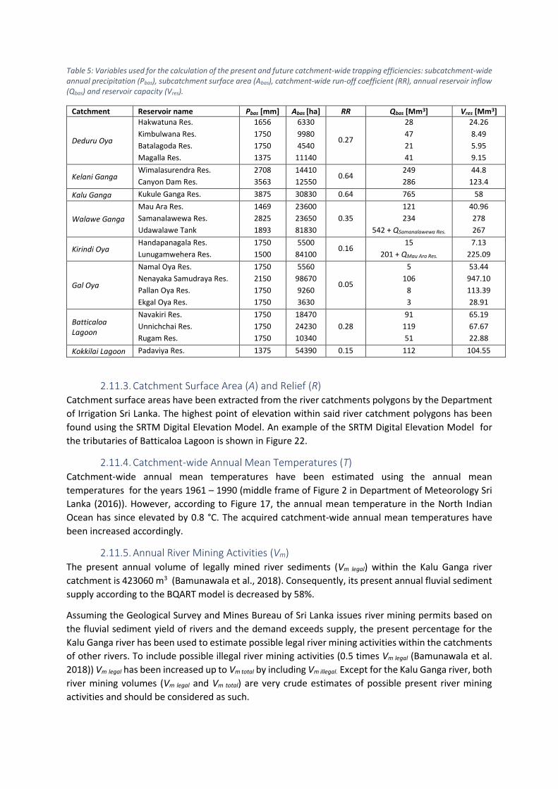
Table 5: Variables used for the calculation of the present and future catchment-wide trapping efficiencies: subcatchment-wide annual precipitation (Pbas), subcatchment surface area (Abas), catchment-wide run-off coefficient (RR), annual reservoir inflow (Qbas) and reservoir capacity (Vres).
Catchment Reservoir name Pbas [mm] Abas [ha] RR Qbas [Mm3] Vres [Mm3]
Deduru Oya
Hakwatuna Res.
Kimbulwana Res.
Batalagoda Res.
Magalla Res.
1656
1750
1750
1375
6330
9980
4540
11140
0.27
28
47
21
41
24.26
8.49
5.95
9.15
Kelani Ganga Wimalasurendra Res.
Canyon Dam Res.
2708
3563
14410
12550 0.64
249
286
44.8
123.4
Kalu Ganga Kukule Ganga Res. 3875 30830 0.64 765 58
Walawe Ganga
Mau Ara Res.
Samanalawewa Res.
Udawalawe Tank
1469
2825
1893
23600
23650
81830
0.35
121
234
542 + QSamanalawewa Res.
40.96
278
267
Kirindi Oya Handapanagala Res.
Lunugamwehera Res.
1750
1500
5500
84100 0.16
15
201 + QMau Ara Res.
7.13
225.09
Gal Oya
Namal Oya Res.
Nenayaka Samudraya Res.
Pallan Oya Res.
Ekgal Oya Res.
1750
2150
1750
1750
5560
98670
9260
3630
0.05
5
106
8
3
53.44
947.10
113.39
28.91
Batticaloa Lagoon
Navakiri Res.
Unnichchai Res.
Rugam Res.
1750
1750
1750
18470
24230
10340
0.28
91
119
51
65.19
67.67
22.88
Kokkilai Lagoon Padaviya Res. 1375 54390 0.15 112 104.55
2.11.3. Catchment Surface Area (A) and Relief (R) Catchment surface areas have been extracted from the river catchments polygons by the Department
of Irrigation Sri Lanka. The highest point of elevation within said river catchment polygons has been
found using the SRTM Digital Elevation Model. An example of the SRTM Digital Elevation Model for
the tributaries of Batticaloa Lagoon is shown in Figure 22.
2.11.4. Catchment-wide Annual Mean Temperatures (T) Catchment-wide annual mean temperatures have been estimated using the annual mean
temperatures for the years 1961 – 1990 (middle frame of Figure 2 in Department of Meteorology Sri
Lanka (2016)). However, according to Figure 17, the annual mean temperature in the North Indian
Ocean has since elevated by 0.8 °C. The acquired catchment-wide annual mean temperatures have
been increased accordingly.
2.11.5. Annual River Mining Activities (Vm) The present annual volume of legally mined river sediments (Vm legal) within the Kalu Ganga river
catchment is 423060 m3 (Bamunawala et al., 2018). Consequently, its present annual fluvial sediment
supply according to the BQART model is decreased by 58%.
Assuming the Geological Survey and Mines Bureau of Sri Lanka issues river mining permits based on
the fluvial sediment yield of rivers and the demand exceeds supply, the present percentage for the
Kalu Ganga river has been used to estimate possible legal river mining activities within the catchments
of other rivers. To include possible illegal river mining activities (0.5 times Vm legal (Bamunawala et al.
2018)) Vm legal has been increased up to Vm total by including Vm illegal. Except for the Kalu Ganga river, both
river mining volumes (Vm legal and Vm total) are very crude estimates of possible present river mining
activities and should be considered as such.

Figure 21: Relative human impact for the tributaries of Batticaloa Lagoon according to the HFPI (Wildlife Conservation Society - WCS and Center for International Earth Science Information Network - CIESIN - Columbia, 2005).
Figure 22: Heights above MSL within the tributaries of Batticaloa Lagoon according to the SRTM Digital Elevation Model (Jarvis et al., 2008).

3. Validity of The Bruun Rule The validity of the Bruun rule in coastline recession studies is often criticised in literature. By answering research question 1:
“What is the validity of applying the Bruun rule in assessing the future position of the Sri Lankan coastline?” this chapter will
provide the reader with information regarding the necessary assumptions and their consequences regarding the validity of a
coastline recession study using the Bruun rule performed for the Sri Lankan coast.
3.1. Limitations to The Use of The Bruun Rule
3.1.1. Availability of Erodible Sediments Firstly, the Bruun rule is only applicable to sandy coastlines. That is, coastlines with enough available
erodible sediments to accommodate an upwards and landwards shift by the active shoreface. This
prerequisite renders the Bruun rule invalid for rocky shorefaces.
Apart from said rocky shorefaces, coastlines protected by means of revetments, jetties, seawalls and
other coastal structures radically depart from the assumptions by the Bruun rule (Zhang et al., 2004).
Similarly, Toimil et al. (2017) carefully select beaches without coastal structures or structures placed
sufficiently far back no influence on coastline recession is expected. In addition, investigating future
beach widths and amongst others the consequences of sea-level rise to the stability of seawalls and
revetments, Udo and Takeda (2017) consider the Bruun rule valid from the present until the moment
in time the landward limit to the active shoreface reaches a (soft) barrier.
3.1.2. Upland Topography Secondly, in their case against the use of the Bruun rule, Cooper and Pilkey (2004) mention the
influence of the slope of the land over which the active shoreface migrates. The Bruun rule assumes
its estimates unaffected, however the amount of recession is easily demonstrated to be inversely
proportional to the upland slope or affected by any upland topography for that matter.
3.1.3. Persistence of an Equilibrium Shaped Active Shoreface Thirdly, in the derivation of the Bruun rule by Zhang et al. (2004) the persistence of the equilibrium
shape of the active shoreface is an important assumption. Consequenly, there are prerequisites
regarding the wave climate and grain size distribution; both constant in time (Cowell et al., 2006; Dean,
1995). Whereas studies regarding the latter are non-existent, projections of the future wave-climates
along the Sri Lankan coast have been found in IPCC (2013) (Table 6). However, together with Nicholls
et al.'s depth of closure estimate, Equation 3 does not allow for the incorporation of changing annual
wave climate variables.
Table 6: Projected change in annual wave climate variables for the Sri Lankan coast according to Figure 13.26 in IPCC (2013).
Annual mean wave climate variables Min. value of change Max. value of change
Significant wave height (Hs) -3% -1%
Wave period (TM) -0.13 s +0.05 s
Wave direction (ϕM) -9° -4°
3.1.4. Coastal Sediment Balance Finally, the Bruun rule describes the redistribution of shoreface sediments and requires the
assumption that no coastal sediments are lost or added to the sediment balance of a beach. CCD (2006)
lists several sinks and sources of which offshore, onshore, and littoral transports of coastal sediments
are considered most important. With the seaward limit to the active shoreface calculated using Nicholl
et al.’s (1996) depth of closure estimate, a constant coastal sediment balance can only be attained by
enforcing zero divergences in the littoral drift of coastal sediments.

3.2. Modifications of The Bruun Rule To decrease the amount of assumptions involved with the application of the Bruun rule, researchers
have presented numerous modifications of the method. Below, a short summary of the more
important modifications is provided.
3.2.1. Upland Topography Komar (1983) presents a generalisation of the Bruun rule applicable to both barrier beaches (found
along the South-east, East and North-east coast of Sri Lanka) and mainlands beaches (found along the
South and South-west coast). Moreover, at mainland beaches, Edelman (1976) employs a variable
berm height to account for the flat topography landward from the berm.
3.2.2. Protected Shorelines From the moment in time the landward limit to the active shoreface reaches a hard barrier and
onwards, Dean (1991) proposes the use of virtual active shoreface origins to determine the scour
affiliated with the persistence of the equilibrium profile. The calculations by Dean (1991) are intricate
and the use of the Bruun principle at shorelines protected by seawalls and revetments is sternly
rejected by Cooper and Pilkey (2004).
3.2.3. Sediment Sinks and Sources A comprehensive effort to incorporate the longshore and cross-shore transports of coastal sediments
through the coastal sediment balance has been made by Cowell et al. (2003). A condensation is found
in Le Cozannet et al. (2016):
𝑅𝑇 =𝐿∗
𝐷𝐶𝛥𝑅𝑆𝐿 + 𝑅𝑐𝑟𝑜𝑠𝑠−𝑠ℎ𝑜𝑟𝑒 + 𝑅𝑙𝑜𝑛𝑔𝑠ℎ𝑜𝑟𝑒 (19)
with Rcross-shore and Rlongshore the horizontal migration by the active shoreface due to respective processes
resulting in the gain or loss of coastal sediments.
Onshore loss of coastal sediments through overwash and aeolian transport may again become
available to the active shoreface as it migrates landward (Jayathilaka, 2015). Therefore, as opposed to
the offshore loss of coastal sediments, subtracting onshore transported coastal sediments from the
coastal sediment balance is a first approximation. To address the onshore loss of coastal sediments
more accurately, Rosati et al. (2013) present a modification of the Bruun rule that includes overwash
and aeolian transport rates.
3.3. Validity of The Bruun Rule along The Sri Lankan Coastline Given the right context, the use of each modification of the Bruun rule is justifiable. However, the
complexity of the calculations, difficulty of delineation correct active shoreface dimensions and/or the
amount of required information increases with each modification employed. Moreover, the
modifications by Komar (1983), Edelman (1976) and Rosati et al. (2013) include the berm height.
To qualitatively adjudge the validity of the Bruun rule (Bruun, 1962), the presence of sink and source
terms for uninterrupted sandy coastlines by Le Cozannet et al. (2016), and for interrupted sandy
coastlines (Ranasinghe et al., 2013) have been mapped (Figure 23). Appendix A provides a textual
explanation per coastal sector.
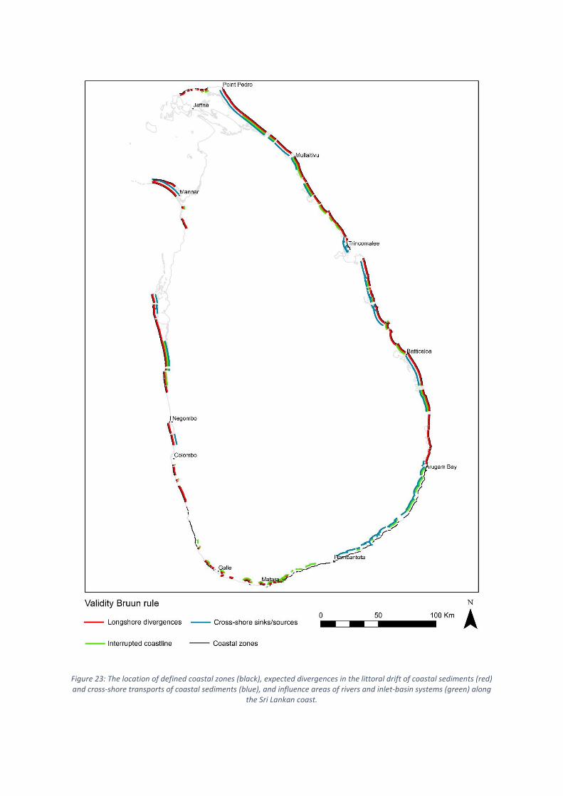
Figure 23: The location of defined coastal zones (black), expected divergences in the littoral drift of coastal sediments (red) and cross-shore transports of coastal sediments (blue), and influence areas of rivers and inlet-basin systems (green) along
the Sri Lankan coast.
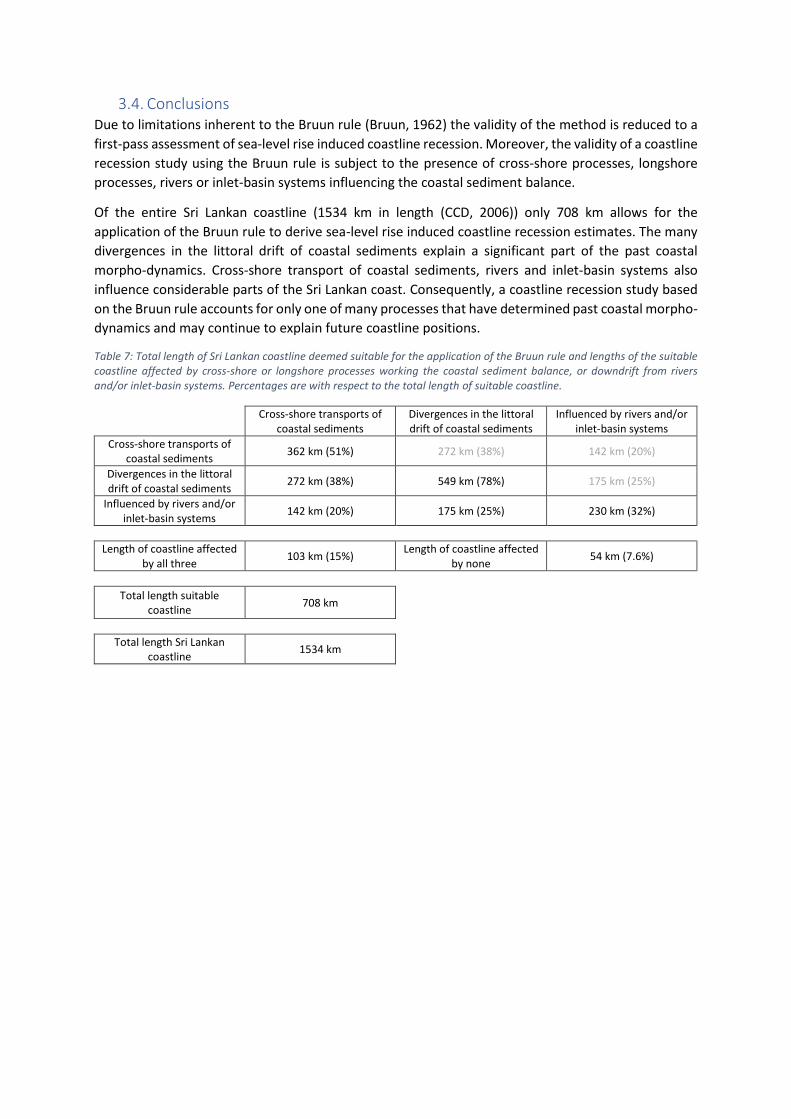
3.4. Conclusions Due to limitations inherent to the Bruun rule (Bruun, 1962) the validity of the method is reduced to a
first-pass assessment of sea-level rise induced coastline recession. Moreover, the validity of a coastline
recession study using the Bruun rule is subject to the presence of cross-shore processes, longshore
processes, rivers or inlet-basin systems influencing the coastal sediment balance.
Of the entire Sri Lankan coastline (1534 km in length (CCD, 2006)) only 708 km allows for the
application of the Bruun rule to derive sea-level rise induced coastline recession estimates. The many
divergences in the littoral drift of coastal sediments explain a significant part of the past coastal
morpho-dynamics. Cross-shore transport of coastal sediments, rivers and inlet-basin systems also
influence considerable parts of the Sri Lankan coast. Consequently, a coastline recession study based
on the Bruun rule accounts for only one of many processes that have determined past coastal morpho-
dynamics and may continue to explain future coastline positions.
Table 7: Total length of Sri Lankan coastline deemed suitable for the application of the Bruun rule and lengths of the suitable coastline affected by cross-shore or longshore processes working the coastal sediment balance, or downdrift from rivers and/or inlet-basin systems. Percentages are with respect to the total length of suitable coastline.
Cross-shore transports of
coastal sediments Divergences in the littoral drift of coastal sediments
Influenced by rivers and/or inlet-basin systems
Cross-shore transports of coastal sediments 362 km (51%) 272 km (38%) 142 km (20%)
Divergences in the littoral drift of coastal sediments 272 km (38%) 549 km (78%) 175 km (25%)
Influenced by rivers and/or inlet-basin systems 142 km (20%) 175 km (25%) 230 km (32%)
Length of coastline affected by all three
103 km (15%) Length of coastline affected
by none 54 km (7.6%)
Total length suitable coastline
708 km
Total length Sri Lankan coastline
1534 km

4. Predictive Accuracy of The Bruun Rule Chapter 4 will seek to provide an answer to research question 2: “What is the predictive accuracy of the Bruun rule for the Sri
Lankan coastline?”. To do so, two comparisons have been performed. Firstly, a hindcast of the Bruun rule for the years 1985
– 2015 using the Satellite Derived Shoreline trends by Luijendijk et al. (2018). Secondly, a comparison between Bruun rule
estimates and Probabilistic Coastal Recession (PCR) method derived coastline recession projections in Dastgheib et al. (2017).
A conclusion has been written including both comparisons at once.
4.1. Bruun Rule Hindcast Hindcasted Bruun rule coastline recession estimates for the years 1985 - 2015 have been compared
with the Satellite Derived Shoreline (SDS) trends by Luijendijk et al. (2018) averaged per defined coastal
zone.
4.1.1. The SDS Dataset The SDS trends have been computed by Luijendijk et al. (2018) using a linear fit to a scatter of cross-
shore satellite derived shoreline locations plotted to the moment in time the measurements have been
taken. Time values are in years with respect to the year 1985. Shoreline locations have been referenced
to an origin landwards from the shoreline. Therefore, a positive trend indicates shoreline progradation.
Figure 24: Satellite derived shoreline trends for every 500m of coastline (Luijendijk et al., 2018) , and calculated average trend per defined coastal zone between Tangalle and Yala.

To arrive at zonal averages, the SDS data points have manually been allocated to the defined coastal
zones. Regarding small defined coastal zones this process is troublesome because the distinction
between a suitable data point (within the reach of a defined coastal zones) and a not suitable data
point (e.g. positioned at a headland) is hard to make. Consequently, defined coastal zones with a small
longshore length have often been omitted. Moreover, defined coastal zones that contain few SDS data
points with respect to their longshore length, have a skewed longshore distribution of SDS data points
or are affected by (updrift) anthropogenic changes to the coast are believed to have distorted SDS
trends and have been excluded as well. Distinguished antropogenic changes are the construction of
harbours, jetties and breakwaters, and beach nourishments. Whereas nourishments performed
without the construction coastal structures may influence multiple downdrift defined coastal zones,
the effect of nourishments combined with coastal structures is believed restricted to the immediate
area.
4.1.2. Results The comparison between past 1985 – 2015 coastline recession trends according to the Bruun rule and
past 1985 – 2015 coastline recession according to the SDS trends has been summarised using a scatter
plot (Figure 25). According to the SDS trend, 60% of the hindcasted coastline (Figure 16) progradated
between the years 1985 and 2015 (bottom half of Figure 25). In general, the receding coastlines are
significantly underestimated by the Bruun rule.
4.1.3. Limitations Verification of the SDS trends using the Uswetakeiyawa 1999 – 2010 erosion study by the CCD was not
successful. Moreover, the SDS trends are based on a linear fit. Thompson et al. (2016) show that past
sea-level rise trends in the North Indian Ocean are non-linear. The used sea-level rise trends have been
calculated matching the approach by Luijendijk et al. (2018) and therefore assume a past linear
increase in sea-level.
Between the years 1985 and 2015, the derived linear sea-level rise trends and affiliated estimated sea-
level rise induced coastline recessions are small. Consequently, it is hard to differentiate the Bruun
principle from other processes (e.g. divergences in the littoral drift of coastal sediments, cross-shore
transports of coastal sediments and interannual variability of storms) (Le Cozannet et al., 2016;
Ranasinghe & Stive, 2009).
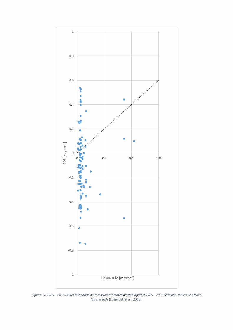
Figure 25: 1985 – 2015 Bruun rule coastline recession estimates plotted against 1985 – 2015 Satellite Derived Shoreline (SDS) trends (Luijendijk et al., 2018).
-1
-0.8
-0.6
-0.4
-0.2
0
0.2
0.4
0.6
0.8
1
0 0.2 0.4 0.6
SDS
[m y
ear-1
]
Bruun rule [m year-1]

4.2. Comparison with The Probabilistic Coastal Recession Method The second comparison will use the stochastic coastline recession projections in Dastgheib et al.
(2017). Said projections have been computed using the Probabilistic Coastal Recession (PCR) method
which is believed more accurate than the Bruun rule (Ranasinghe et al., 2012). Spanning 85 transects
in 72 km of uninterrupted coastline (Figure 26), the work by Dastgheib et al. (2017) incorporates
steeply and mildly sloping shorefaces, and shorefaces with various berm heights.
Since Ranasinghe and Stive (2009), and Zhang et al. (2004) state that the Bruun rule is only capable of
providing an average coastline recession estimates for defined coastal zones, the comparison between
the Bruun rule and the PCR method has been performed on both a transect and a zonal basis. Zonal
Bruun rule coastline recession estimates have been calculated using average cross-shore profiles and
PCR projections have been averaged for each coastal zone delineated by Dastgheib et al. (2017) (Figure
26).
Figure 26: Spatial scope of the two study areas Tincomalee – Kuchchaveli (left frame) and Karaitivu – Batticaloa (right frame). Coastal zones defined by Dastgheib et al. (2017) have been numbered and the positions of transects part of the PCR
analysis are shown using dots (Dastgheib et al., 2017).
4.2.1. The PCR Method The PCR method is a process based model that can be used to attain stochastic coastline recession
projections. The PCR method believes present coastline positions the result of storm eroding the beach
and beach recovery and sea-level rise induced coastline recession the result of both inundation and
the increase of beach erosion due to an increased exposure to storms (Ranasinghe et al., 2012).
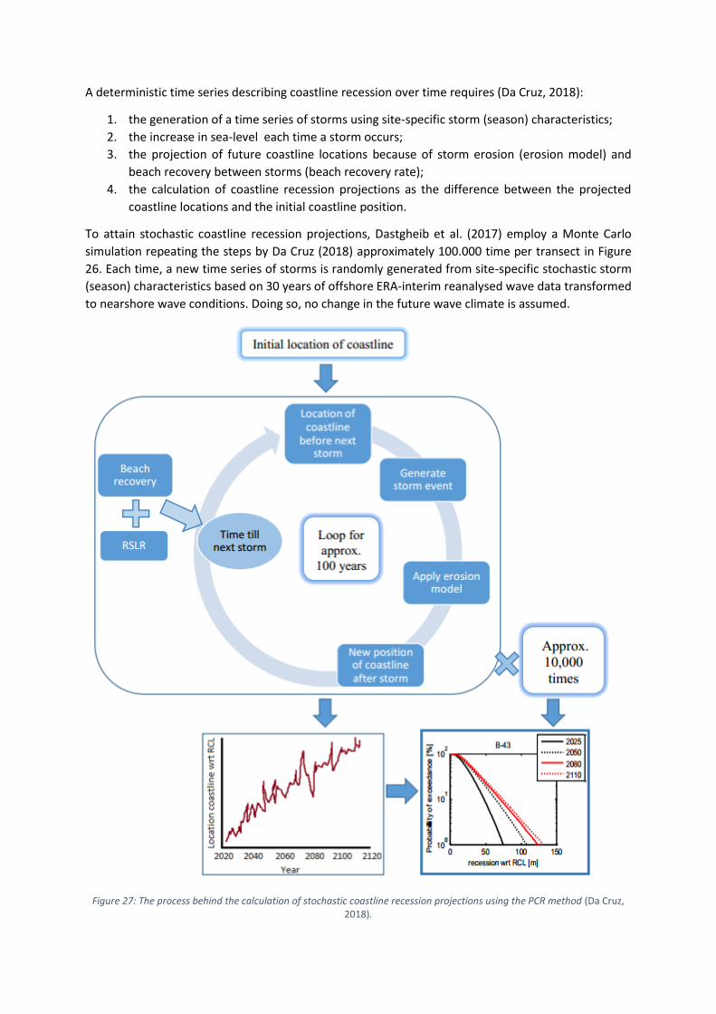
A deterministic time series describing coastline recession over time requires (Da Cruz, 2018):
1. the generation of a time series of storms using site-specific storm (season) characteristics;
2. the increase in sea-level each time a storm occurs;
3. the projection of future coastline locations because of storm erosion (erosion model) and
beach recovery between storms (beach recovery rate);
4. the calculation of coastline recession projections as the difference between the projected
coastline locations and the initial coastline position.
To attain stochastic coastline recession projections, Dastgheib et al. (2017) employ a Monte Carlo
simulation repeating the steps by Da Cruz (2018) approximately 100.000 time per transect in Figure
26. Each time, a new time series of storms is randomly generated from site-specific stochastic storm
(season) characteristics based on 30 years of offshore ERA-interim reanalysed wave data transformed
to nearshore wave conditions. Doing so, no change in the future wave climate is assumed.
Figure 27: The process behind the calculation of stochastic coastline recession projections using the PCR method (Da Cruz, 2018).

4.2.1.1. Erosion model
Several erosion models can be applied to derive erosion volumes from storm conditions (Da Cruz,
2018). In Dastgheib et al. (2017) the predictive function by Mendoza and Jiménez (2006) is employed:
∆𝑉 = 𝐶1 𝐽𝐴 𝑑𝑡 + 𝐶2 (20)
with C1 and C2 model parameters calibrated for each defined coastal zone in Figure 26 and JA a
predictor (Jiménez et al., 1993), which includes the beach slope. Beach slopes have been measured
from recent surveys by the CCD.
4.2.1.2. Interpretation of PCR method derived coastline recession projections
An empirical cumulative distribution function is fitted to the results of the Monte Carlo analysis.
Exceedance probabilities (vertical axis in the bottom right frame of Figure 27) depict the chance that
the annual position of the shoreline is landward from a certain distance to the reference coastline
(horizontal axis in the bottom right frame of Figure 27) at a certain year. In Dastgheib et al. (2017) the
annual position corresponds with the maximum recorded distance to the reference coastline. High
exceedance probabilities equal small coastline recession projections and low exceedance probabilities
equal large coastline recession projections. Here the exceedance probability (10%, 50% or 99%) and
the year (2050 or 2110) are defined, and the corresponding projected position of the shoreline is
sought.
4.2.1.3. Horizontal Migration of The MSL Mark
The PCR projections in Dastgheib et al. (2017) depict the future position of the MSL mark with respect
to the past 1% probabilistic wave runup line during 30 years of simulations. With the Bruun rule
estimate the landward migration of the MSL mark, the PCR projections must be modified to express
the same value. Consequently, additional information regarding the exact geographic location of the
MSL mark in the PCR projections, the cross-shore position of the MSL in the profile drawings used in
the PCR analysis, the exact geographic location of the origin in the profile drawings and the distance
between the PCR projections and the transect origin is required.
4.2.2. Results According to Figure 28, the 2110 annual landward migration of the MSL mark exceeded in 50% of the
PCR method runs is always greater than the coastline recession estimate provided by the Bruun rule.
The underestimation of by the Bruun rule persists into the highest (99%) exceedance probability.
Differences between the Bruun rule coastline recession estimates and the PCR method projections
increase with shorter timescales (Figure 29).
The variability in the 2110 PCR method derived coastline recessions associated with 50% probability of
occurrence devided by the 2110 Bruun rule coastline recession estimate scatter is best reduced by
substracting an exponential line based on the slope of the active shoreface. The remaining variability
can be decreased further by taking the zonal averages (Figure 30). The relative difference between the
PCR method and the Bruun rule increases with approximately the same magnitude as the slope of the
active shoreface. Creating the same plots for the 2110 PCR method derived coastline recessions
associated with 99% probability of occurance results in a ‘consistent’ (0 - 50%) relative underestimation
of the PCR method results by the Bruun rule (Figure 31).

Figure 28: 10% (orange), 50% (blue) and 99% probabilistic coastal recession projections according to the PCR method for the year 2110 plotted against the 2110 Bruun rule coastline recession estimates.
Figure 29: 10% (orange), 50% (blue) and 99% probabilistic coastal recession projections according to the PCR method for the year 2050 plotted against the 2050 Bruun rule coastline recession estimates.
0
25
50
75
100
125
150
175
0 25 50 75 100 125 150 175
PC
R p
roje
ctio
n [
m]
Bruun estimate [m]
2110 scatter
10% PCR 50% PCR 99% PCR
-25
0
25
50
75
100
125
150
0 25 50 75 100 125 150 175
PC
R p
roje
ctio
n [
m]
Bruun rule estimate [m]
2050 scatter
10% PCR 50% PCR 99% PCR

Figure 30: 50% probabilistic coastal recession projections for the year 2110/2110 Bruun rule coastline recession estimate ratios for defined coastal zones (squares) T1, T2, T3, T4, T5, B1, B2, B3 and B4 plotted against their average active shoreface
slope. Ratios of their separate transects have been included using bullets.
Figure 31: 99% probabilistic coastal recession projections for the year 2110/2110 Bruun rule coastline recession estimate ratios for coastal zones (squares) T1, T2, T3, T4, T5, B1, B2, B3 and B4 plotted against their average active shoreface slope.
Ratios of their separate transects have been included using bullets.
R² = 0.6601
1
2
3
4
5
6
7
0 0.01 0.02 0.03 0.04 0.05 0.06
50
% P
CR
pro
ject
ion
/Bru
un
ru
le e
stim
ate
tan(β)
2110 ratio
T1
T2
T3
T4
T5
B1
B2
B3
B4
0
1
2
3
4
5
6
7
0 0.01 0.02 0.03 0.04 0.05 0.06
99
% P
CR
pro
ject
ion
/Bru
un
ru
le e
stim
ate
tan(β)
2110 ratio
T1
T2
T3
T4
T5
B1
B2
B3
B4
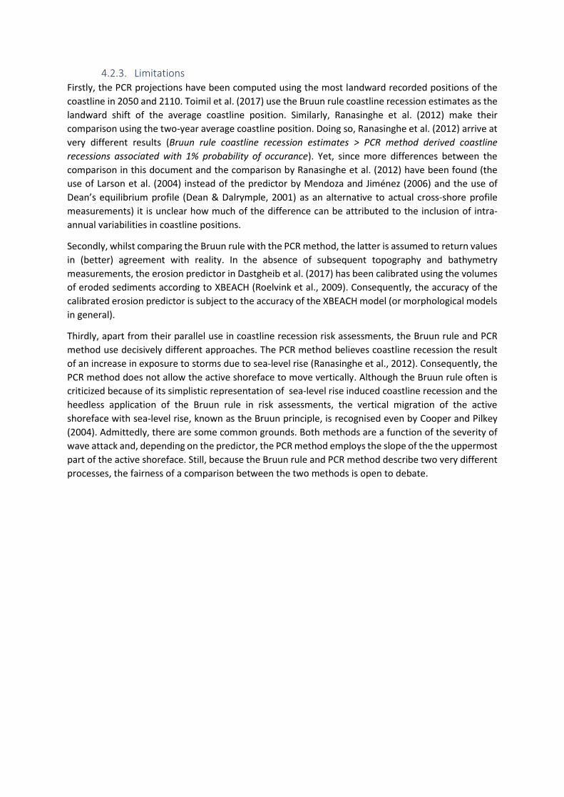
4.2.3. Limitations Firstly, the PCR projections have been computed using the most landward recorded positions of the
coastline in 2050 and 2110. Toimil et al. (2017) use the Bruun rule coastline recession estimates as the
landward shift of the average coastline position. Similarly, Ranasinghe et al. (2012) make their
comparison using the two-year average coastline position. Doing so, Ranasinghe et al. (2012) arrive at
very different results (Bruun rule coastline recession estimates > PCR method derived coastline
recessions associated with 1% probability of occurance). Yet, since more differences between the
comparison in this document and the comparison by Ranasinghe et al. (2012) have been found (the
use of Larson et al. (2004) instead of the predictor by Mendoza and Jiménez (2006) and the use of
Dean’s equilibrium profile (Dean & Dalrymple, 2001) as an alternative to actual cross-shore profile
measurements) it is unclear how much of the difference can be attributed to the inclusion of intra-
annual variabilities in coastline positions.
Secondly, whilst comparing the Bruun rule with the PCR method, the latter is assumed to return values
in (better) agreement with reality. In the absence of subsequent topography and bathymetry
measurements, the erosion predictor in Dastgheib et al. (2017) has been calibrated using the volumes
of eroded sediments according to XBEACH (Roelvink et al., 2009). Consequently, the accuracy of the
calibrated erosion predictor is subject to the accuracy of the XBEACH model (or morphological models
in general).
Thirdly, apart from their parallel use in coastline recession risk assessments, the Bruun rule and PCR
method use decisively different approaches. The PCR method believes coastline recession the result
of an increase in exposure to storms due to sea-level rise (Ranasinghe et al., 2012). Consequently, the
PCR method does not allow the active shoreface to move vertically. Although the Bruun rule often is
criticized because of its simplistic representation of sea-level rise induced coastline recession and the
heedless application of the Bruun rule in risk assessments, the vertical migration of the active
shoreface with sea-level rise, known as the Bruun principle, is recognised even by Cooper and Pilkey
(2004). Admittedly, there are some common grounds. Both methods are a function of the severity of
wave attack and, depending on the predictor, the PCR method employs the slope of the the uppermost
part of the active shoreface. Still, because the Bruun rule and PCR method describe two very different
processes, the fairness of a comparison between the two methods is open to debate.

4.3. Conclusions
The predictive accuracy of the Bruun rule depends on the interpretation of the Bruun rule coastline
recession estimates.
Reasonably probable future annual coastline locations appear mostly the result of annual storm
erosion instead of sea-level rise induced coastline recession described by the the Bruun principle.With
regard to the accuracy of the Bruun rule in predicting the sea-level rise induced recession of the
average position of the coastline, the Bruun rule hindcast and the comparison between the Bruun rule
coastline recession estimates and the PCR method results in Dastgheib et al. (2017) are inconclusive.
The accuracy of the SDS dataset could not be verified and the linear fit used by the SDS dataset does
not recognise the non-linear increase in sea-level between the years 1985 and 2015. Moreover, the
Bruun principle is likely obscured by other local scale processes that have determined past coastline
positions. Bruun rule coastline recession estimates show better agreement with high exceedance
probability PCR method derived coastline recessions and said high exceedance probability projections
are more comparable to the average location of the coastline than the low exceedance probability
projections. However, the difference between the average coastline position and the definition of the
annual location of the coastline in Dastgheib et al. (2017) cannot be bridged.
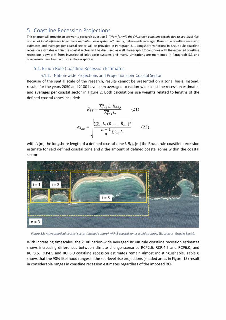
5. Coastline Recession Projections This chapter will provide an answer to research question 3: “How far will the Sri Lankan coastline recede due to sea-level rise,
and what local influence have rivers and inlet-basin systems?”. Firstly, nation-wide averaged Bruun rule coastline recession
estimates and averages per coastal sector will be provided in Paragraph 5.1. Longshore variations in Bruun rule coastline
recession estimates within the coastal sectors will be discussed as well. Paragraph 5.2 continues with the expected coastline
recessions downdrift from investigated inlet-basin systems and rivers. Limitations are mentioned in Paragraph 5.3 and
conclusions have been written in Paragraph 5.4.
5.1. Bruun Rule Coastline Recession Estimates
5.1.1. Nation-wide Projections and Projections per Coastal Sector Because of the spatial scale of the research, results cannot be presented on a zonal basis. Instead,
results for the years 2050 and 2100 have been averaged to nation-wide coastline recession estimates
and averages per coastal sector in Figure 2. Both calculations use weights related to lengths of the
defined coastal zones included:
�̅�𝐵𝐸 =∑ 𝐿𝑖 𝑅𝐵𝐸,𝑖
𝑛𝑖=1
∑ 𝐿𝑖𝑛𝑖=1
(21)
𝜎𝑅𝐵𝐸= √
∑ 𝐿𝑖 (𝑅𝐵𝐸 − �̅�𝐵𝐸)2𝑛𝑖=1
𝑛 − 1𝑛
∑ 𝐿𝑖𝑛𝑖=1
(22)
with Li [m] the longshore length of a defined coastal zone i, RBE,i [m] the Bruun rule coastline recession
estimate for said defined coastal zone and n the amount of defined coastal zones within the coastal
sector.
Figure 32: A hypothetical coastal sector (dashed square) with 3 coastal zones (solid squares) (Baselayer: Google Earth).
With increasing timescales, the 2100 nation-wide averaged Bruun rule coastline recession estimates
shows increasing differences between climate change scenarios RCP2.6, RCP.4.5 and RCP6.0, and
RCP8.5. RCP4.5 and RCP6.0 coastline recession estimates remain almost indistinguishable. Table 8
shows that the 90% likelihood ranges in the sea-level rise projections (shaded areas in Figure 13) result
in considerable ranges in coastline recession estimates regardless of the imposed RCP.
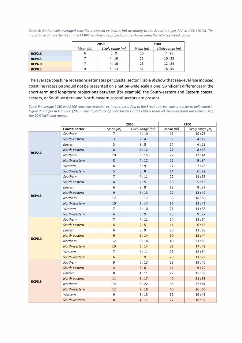
Table 8: Nation-wide averaged coastline recession estimates [m] according to the Bruun rule per RCP in IPCC (2013). The importance of uncertainties in the CMIP5 sea-level rise projections are shown using the 90% likelihood ranges.
2050 2100
Mean [m] Likely range [m] Mean [m] Likely range [m]
RCP2.6 6 3 : 9 16 7 : 25
RCP4.5 7 4 : 10 21 10 : 32
RCP6.0 7 4 : 10 23 12 : 34
RCP8.5 9 5 : 13 31 18 : 45
The average coastline recessions estimates per coastal sector (Table 9) show that sea-level rise induced
coastline recession should not be presented on a nation-wide scale alone. Significant differences in the
short-term and long-term projections between (for example) the South-eastern and Eastern coastal
sectors, or South-eastern and North-eastern coastal sectors are present.
Table 9: Average 2050 and 2100 coastline recession estimates according to the Bruun rule per coastal sector as delineated in Figure 2 and per RCP in IPCC (2013). The importance of uncertainties in the CMIP5 sea-level rise projections are shown using the 90% likelihood ranges.
2050 2100
Coastal sector Mean [m] Likely range [m] Mean [m] Likely range [m]
RCP2.6
Southern 7 4 : 10 17 10 : 26
South-eastern 3 2 : 4 8 4 : 12
Eastern 5 3 : 8 14 6 : 22
North-eastern 8 4 : 12 21 8 : 33
Northern 10 5 : 15 27 12 : 41
North-western 8 4 : 12 22 9 : 34
Western 6 3 : 9 17 7 : 26
South-western 5 3 : 8 14 6 : 22
RCP4.5
Southern 7 4 : 11 22 11 : 33
South-eastern 4 2 : 5 10 5 : 15
Eastern 6 3 : 9 18 9 : 27
North-eastern 9 5 : 13 27 13 : 42
Northern 12 6 : 17 36 18 : 56
North-western 10 5 : 14 30 15 : 45
Western 7 4 : 10 21 11 : 33
South-western 6 3 : 9 18 9 : 27
RCP6.0
Southern 7 4 : 11 24 13 : 34
South-eastern 4 2 : 5 11 6 : 16
Eastern 6 3 : 9 20 11 : 29
North-eastern 9 5 : 14 30 15 : 44
Northern 12 6 : 18 40 21 : 59
North-western 10 5 : 14 32 17 : 48
Western 7 4 : 11 23 12 : 34
South-western 6 3 : 9 20 11 : 29
RCP8.5
Southern 9 5 : 13 32 19 : 45
South-eastern 4 3 : 6 15 9 : 22
Eastern 8 4 : 11 27 15 : 38
North-eastern 11 6 : 17 40 21 : 58
Northern 15 8 : 22 56 32 : 81
North-western 12 7 : 18 46 26 : 66
Western 9 5 : 13 32 19 : 46
South-western 8 4 : 11 27 16 : 38
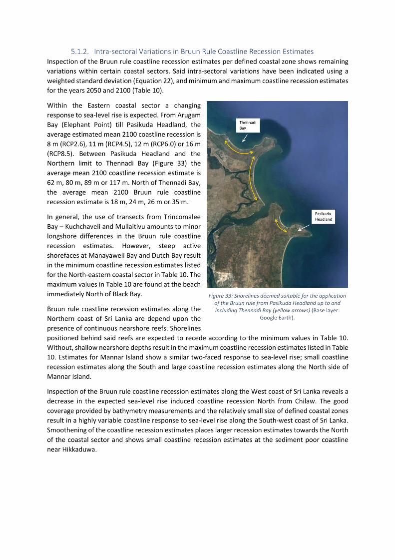
5.1.2. Intra-sectoral Variations in Bruun Rule Coastline Recession Estimates Inspection of the Bruun rule coastline recession estimates per defined coastal zone shows remaining
variations within certain coastal sectors. Said intra-sectoral variations have been indicated using a
weighted standard deviation (Equation 22), and minimum and maximum coastline recession estimates
for the years 2050 and 2100 (Table 10).
Within the Eastern coastal sector a changing
response to sea-level rise is expected. From Arugam
Bay (Elephant Point) till Pasikuda Headland, the
average estimated mean 2100 coastline recession is
8 m (RCP2.6), 11 m (RCP4.5), 12 m (RCP6.0) or 16 m
(RCP8.5). Between Pasikuda Headland and the
Northern limit to Thennadi Bay (Figure 33) the
average mean 2100 coastline recession estimate is
62 m, 80 m, 89 m or 117 m. North of Thennadi Bay,
the average mean 2100 Bruun rule coastline
recession estimate is 18 m, 24 m, 26 m or 35 m.
In general, the use of transects from Trincomalee
Bay – Kuchchaveli and Mullaitivu amounts to minor
longshore differences in the Bruun rule coastline
recession estimates. However, steep active
shorefaces at Manayaweli Bay and Dutch Bay result
in the minimum coastline recession estimates listed
for the North-eastern coastal sector in Table 10. The
maximum values in Table 10 are found at the beach
immediately North of Black Bay.
Bruun rule coastline recession estimates along the
Northern coast of Sri Lanka are depend upon the
presence of continuous nearshore reefs. Shorelines
positioned behind said reefs are expected to recede according to the minimum values in Table 10.
Without, shallow nearshore depths result in the maximum coastline recession estimates listed in Table
10. Estimates for Mannar Island show a similar two-faced response to sea-level rise; small coastline
recession estimates along the South and large coastline recession estimates along the North side of
Mannar Island.
Inspection of the Bruun rule coastline recession estimates along the West coast of Sri Lanka reveals a
decrease in the expected sea-level rise induced coastline recession North from Chilaw. The good
coverage provided by bathymetry measurements and the relatively small size of defined coastal zones
result in a highly variable coastline response to sea-level rise along the South-west coast of Sri Lanka.
Smoothening of the coastline recession estimates places larger recession estimates towards the North
of the coastal sector and shows small coastline recession estimates at the sediment poor coastline
near Hikkaduwa.
Figure 33: Shorelines deemed suitable for the application of the Bruun rule from Pasikuda Headland up to and including Thennadi Bay (yellow arrows) (Base layer:
Google Earth).

Table 10: Intra-sectoral variations in the Bruun rule coastline recession estimates per RCP in IPCC (2013) shown using the minimum and maximum mean coastline recession estimates, and the weighted standard deviation of the mean coastline recession estimates. The standard deviations for coastal sectors with few transects have been greyed out.
2050 2100
Coastal sector Standard deviation [m]
Min : Max recession [m]
Standard deviation [m]
Min : Max recession [m]
RCP2.6
Southern 0.9 4 : 7 2.3 9 : 18
South-eastern 0.3 2 : 6 0.9 6 : 15
Eastern 5.1 2 : 30 13.6 5 : 81
North-eastern 1.3 4 : 13 3.5 12 : 34
Northern 5.9 6 : 18 15.9 16 : 48
North-western 6.4 3 : 17 17.3 9 : 45
Western 1.8 2 : 11 4.9 4 : 29
South-western 1.8 2 : 9 4.7 6 : 23
RCP4.5
Southern 1.0 4 : 8 2.9 12 : 23
South-eastern 0.4 3 : 7 1.1 8 : 19
Eastern 5.9 2 : 35 17.5 7 : 104
North-eastern 1.6 4 : 15 4.5 15 : 44
Northern 7.1 7 : 21 21.7 21 : 65
North-western 7.7 4 : 20 23.6 12 : 61
Western 2.1 2 : 13 6.1 5 : 37
South-western 2.0 3 : 10 6.0 8 : 30
RCP6.0
Southern 1.0 4 : 8 3.2 13 : 25
South-eastern 0.4 3 : 7 1.3 9 : 21
Eastern 6.2 2 : 37 19.4 7 : 115
North-eastern 1.7 5 : 17 5.1 17 : 49
Northern 7.1 7 : 22 23.7 23 : 71
North-western 7.8 3 : 20 25.9 13 : 67
Western 2.1 2 : 13 6.7 6 : 40
South-western 2.1 3 : 10 6.6 8 : 32
RCP8.5
Southern 1.2 5 : 10 4.2 18 : 34
South-eastern 0.5 3 : 8 1.7 12 : 29
Eastern 7.3 3 : 43 25.5 10 : 152
North-eastern 1.9 6 : 22 6.3 23 : 65
Northern 8.9 9 : 27 33.3 32 : 100
North-western 9.7 5 : 25 36.2 19 : 94
Western 2.6 2 : 16 9.0 8 : 55
South-western 2.6 3 : 12 8.9 12 : 44
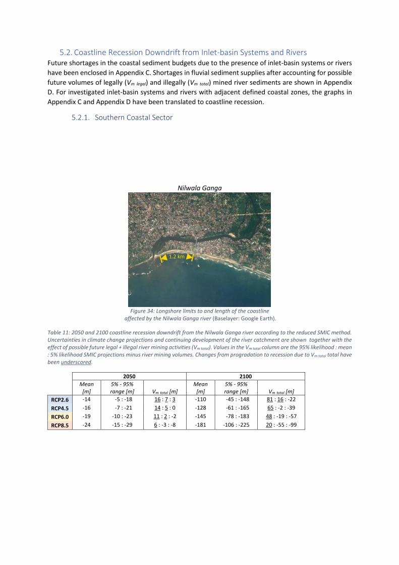
5.2. Coastline Recession Downdrift from Inlet-basin Systems and Rivers Future shortages in the coastal sediment budgets due to the presence of inlet-basin systems or rivers
have been enclosed in Appendix C. Shortages in fluvial sediment supplies after accounting for possible
future volumes of legally (Vm legal) and illegally (Vm total) mined river sediments are shown in Appendix
D. For investigated inlet-basin systems and rivers with adjacent defined coastal zones, the graphs in
Appendix C and Appendix D have been translated to coastline recession.
5.2.1. Southern Coastal Sector
Nilwala Ganga
Figure 34: Longshore limits to and length of the coastline
affected by the Nilwala Ganga river (Baselayer: Google Earth).
Table 11: 2050 and 2100 coastline recession downdrift from the Nilwala Ganga river according to the reduced SMIC method. Uncertainties in climate change projections and continuing development of the river catchment are shown together with the effect of possible future legal + illegal river mining activities (Vm total). Values in the Vm total column are the 95% likelihood : mean : 5% likelihood SMIC projections minus river mining volumes. Changes from progradation to recession due to Vm total total have been underscored.
2050 2100
Mean [m]
5% - 95% range [m] Vm total [m]
Mean [m]
5% - 95% range [m] Vm total [m]
RCP2.6 -14 -5 : -18 16 : 7 : 3 -110 -45 : -148 81 : 16 : -22
RCP4.5 -16 -7 : -21 14 : 5 : 0 -128 -61 : -165 65 : -2 : -39
RCP6.0 -19 -10 : -23 11 : 2 : -2 -145 -78 : -183 48 : -19 : -57
RCP8.5 -24 -15 : -29 6 : -3 : -8 -181 -106 : -225 20 : -55 : -99

5.2.2. South-eastern Coastal Sector
Kirindi Oya
Menik Ganga
Kumbukkan Oya
Figure 35: Longshore limits to and lengths of the coastlines affected by the Kirindi Oya, Menik Ganga and Kumbukkan Oya
rivers (Baselayer: Google Earth).
Table 12: 2050 and 2100 coastline recession downdrift from the Kirindi Oya, Menik Ganga and Kumbukkan Oya rivers according to the reduced SMIC method. Uncertainties in climate change projections and continuing development of the rivers catchments are shown together with the effect of possible future legal + illegal river mining activities (Vm total). Values in the Vm total column are the 95% likelihood : mean : 5% likelihood SMIC projections minus river mining volumes. Changes from progradation to recession due to Vm total total have been underscored.
2050 2100
River
Mean [m]
5% - 95% range [m] Vm total [m]
Mean [m]
5% - 95% range [m] Vm total [m]
RCP2.6
Kirindi Oya -1 0 : -1 - -16 -8 : -20 -
Menik Ganga -1 0 : -1 4 : 3 : 3 -17 -9 : -21 12 : 4 : 0
Kumbukkan Oya -5 -2 : -6 5 : 2 : 1 -40 -19 : -52 22 : 1 : -11
RCP4.5
Kirindi Oya -1 -1 : -1 - -18 -9 : -21 -
Menik Ganga -1 -1 : -1 3 : 3 : 3 -19 -10 : -22 11 : 2 : -1
Kumbukkan Oya -5 -3 : -7 4 : 2 : 0 -45 -23 : -57 18 : -4 : -16
RCP6.0
Kirindi Oya -2 -2 : -2 - -25 -16 : -29 -
Menik Ganga -2 -2 : -2 2 : 2 : 2 -28 -19 : -32 2 : -7 : -11
Kumbukkan Oya -8 -5 : -9 2 : -1 : -2 -61 -39 : -74 2 : -20 : -33
RCP8.5
Kirindi Oya -3 -3 : -3 - -34 -24 : -38 -
Menik Ganga -4 -4 : -4 0 : 0 : 0 -39 -28 : -43 -7 : -18 : -22
Kumbukkan Oya -11 -8 : -13 -1 : -4 : -6 -83 -57 : -97 -16 : -42 : -56

5.2.3. Eastern Coastal Sector
Gal Oya
Batticaloa Lagoon
Figure 36: Longshore limits to and lengths of the coastlines affected by the Gal Oya river and Batticaloa Lagoon (Baselayer: Google Earth).
Table 13: 2050 and 2100 coastline recession downdrift from the Gal Oya river and Batticaloa Lagoon according to the (reduced) SMIC method. Uncertainties in climate change projections and continuing development of the Gal Oya river and the tributaries of Batticaloa lagoon are shown shown together with the effect of possible future legal + illegal river mining activities (Vm total). Values in the Vm total column are the 95% likelihood : mean : 5% likelihood SMIC projections minus river mining volumes. Changes from progradation to recession due to Vm total total have been underscored.
2050 2100
Inlet-basin system/River
Mean [m]
5% - 95% range [m] Vm total [m]
Mean [m]
5% - 95% range [m] Vm total [m]
RCP2.6 Gal Oya 2 1 : 3 - 5 2 : 7 -
Batticaloa Lagoon 89 39 : 142 41 :91 : 144 223 80 : 368 92 : 235 : 380
RCP4.5 Gal Oya 3 2 : 4 - 7 4 : 10 -
Batticaloa Lagoon 104 51 : 156 53 : 106 : 158 291 134 : 459 146 : 303 : 471
RCP6.0 Gal Oya 3 1 : 4 - 6 3 : 9 -
Batticaloa Lagoon 103 49 : 159 51 : 105 : 161 310 149 : 476 161 : 322 : 488
RCP8.5 Gal Oya 3 2 : 4 - 8 4 : 13 -
Batticaloa Lagoon 119 56 : 181 58 : 121 : 183 405 213 : 610 225 : 417 : 622

5.2.4. North-eastern Coastal Sector
Kokkilai Lagoon
Nayaru Lagoon
Figure 37: Longshore limits to and lengths of the coastlines affected by Kokkilai Lagoon and Nayaru Lagoon (Baselayer:
Google Earth).
Table 14: 2050 and 2100 coastline recession downdrift from Kokkilai Lagoon and Nayaru Lagoon according to the SMIC method. Uncertainties in climate change projections and continuing development of tributaries are shown together with the effect of possible future legal + illegal river mining activities (Vm total). Values in the Vm total column are the 95% likelihood : mean : 5% likelihood SMIC projections minus river mining volumes. Changes from progradation to recession due to Vm total total have been underscored.
2050 2100
Inlet-basin system
Mean [m]
5% - 95% range [m] Vm total [m]
Mean [m]
5% - 95% range [m] Vm total [m]
RCP2.6 Kokkilai Lagoon 45 22 : 69 22 : 45 : 69 119 50 : 187 52 : 121 : 189
Nayaru Lagoon 8 4 : 12 4 : 8 : 12 21 8 : 34 8 : 21 : 34
RCP4.5 Kokkilai Lagoon 52 27 : 76 27 : 52 : 76 153 75 : 235 77 : 155 : 237
Nayaru Lagoon 9 5 : 13 5 : 9 : 13 27 13 : 44 13 : 27 : 44
RCP6.0 Kokkilai Lagoon 52 27 : 77 27 : 52 : 77 164 85 : 244 87 : 166 : 246
Nayaru Lagoon 9 4 : 13 4 : 9 : 13 29 15 : 46 15 : 29 : 46
RCP8.5 Kokkilai Lagoon 64 34 : 93 64 : 34 : 93 225 128 : 326 130 : 227 : 328
Nayaru Lagoon 11 6 : 16 6 : 11 : 16 42 23 : 63 23 : 42 : 63

5.2.5. Northern Coastal Sector
Thondammanaru Lagoon
Figure 38: Longshore limits to and length of the coastline
affected by Thondammanaru Lagoon (Baselayer: Google Earth).
Table 15: 2050 and 2100 coastline recession downdrift from Thondammanaru Lagoon according to the SMIC method.
2050 2100
Mean [m]
5% – 95% range [m]
Mean [m]
5% - 95% range [m]
RCP2.6 -134 -70 : -193 -333 -155 : -459
RCP4.5 -159 -85 : -227 -424 -231 : -506
RCP6.0 -160 -84 : -232 -450 -267 : -508
RCP8.5 -197 -109 : -278 -506 -386 : -444
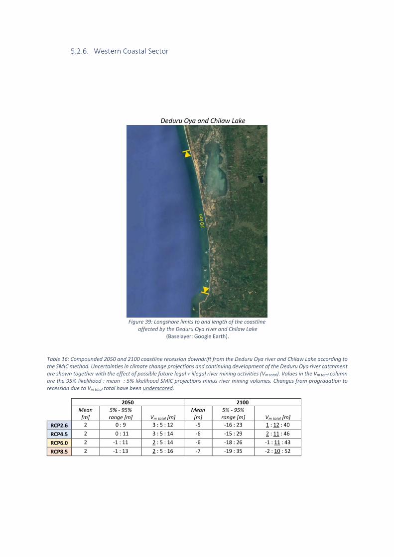
5.2.6. Western Coastal Sector
Deduru Oya and Chilaw Lake
Figure 39: Longshore limits to and length of the coastline
affected by the Deduru Oya river and Chilaw Lake (Baselayer: Google Earth).
Table 16: Compounded 2050 and 2100 coastline recession downdrift from the Deduru Oya river and Chilaw Lake according to the SMIC method. Uncertainties in climate change projections and continuing development of the Deduru Oya river catchment are shown together with the effect of possible future legal + illegal river mining activities (Vm total). Values in the Vm total column are the 95% likelihood : mean : 5% likelihood SMIC projections minus river mining volumes. Changes from progradation to recession due to Vm total total have been underscored.
2050 2100
Mean [m]
5% - 95% range [m] Vm total [m]
Mean [m]
5% - 95% range [m] Vm total [m]
RCP2.6 2 0 : 9 3 : 5 : 12 -5 -16 : 23 1 : 12 : 40
RCP4.5 2 0 : 11 3 : 5 : 14 -6 -15 : 29 2 : 11 : 46
RCP6.0 2 -1 : 11 2 : 5 : 14 -6 -18 : 26 -1 : 11 : 43
RCP8.5 2 -1 : 13 2 : 5 : 16 -7 -19 : 35 -2 : 10 : 52
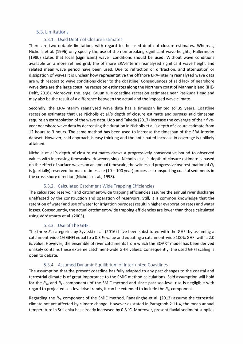
5.3. Limitations
5.3.1. Used Depth of Closure Estimates There are two notable limitations with regard to the used depth of closure estimates. Whereas,
Nicholls et al. (1996) only specify the use of the non-breaking significant wave heights, Hallermeier
(1980) states that local (significant) wave conditions should be used. Without wave conditions
available on a more refined grid, the offshore ERA-Interim reanalysed significant wave height and
related mean wave period have been used. Due to refraction or diffraction, and attenuation or
dissipation of waves it is unclear how representative the offshore ERA-Interim reanalysed wave data
are with respect to wave conditions closer to the coastline. Consequences of said lack of nearshore
wave data are the large coastline recession estimates along the Northern coast of Mannar Island (IHE-
Delft, 2016). Moreover, the large Bruun rule coastline recession estimates near Pasikuda Headland
may also be the result of a difference between the actual and the imposed wave climate.
Secondly, the ERA-Interim reanalysed wave data has a timespan limited to 35 years. Coastline
recession estimates that use Nicholls et al.’s depth of closure estimate and surpass said timespan
require an extrapolation of the wave data. Udo and Takeda (2017) increase the coverage of their five-
year nearshore wave data by decreasing the duration in Nicholls et al.’s depth of closure estimate from
12 hours to 3 hours. The same method has been used to increase the timespan of the ERA-Interim
dataset. However, said approach is easy thinking and the anticipated increase in coverage is unlikely
attained.
Nicholls et al.’s depth of closure estimates draws a progressively conservative bound to observed
values with increasing timescales. However, since Nicholls et al.’s depth of closure estimate is based
on the effect of surface waves on an annual timescale, the witnessed progressive overestimation of DC
is (partially) reserved for macro timescale (10 – 100 year) processes transporting coastal sediments in
the cross-shore direction (Nicholls et al., 1998).
5.3.2. Calculated Catchment Wide Trapping Efficiencies The calculated reservoir and catchment-wide trapping efficiencies assume the annual river discharge
unaffected by the construction and operation of reservoirs. Still, it is common knowledge that the
retention of water and use of water for irrigation purposes result in higher evaporation rates and water
losses. Consequently, the actual catchment-wide trapping efficiencies are lower than those calculated
using Vörösmarty et al. (2003).
5.3.3. Use of The GHFI The three Eh categories by Syvitski et al. (2016) have been substituted with the GHFI by assuming a
catchment-wide 1% GHFI equal to a 0.3 Eh value and equating a catchment-wide 100% GHFI with a 2.0
Eh value. However, the ensemble of river catchments from which the BQART model has been derived
unlikely contains these extreme catchment-wide GHFI values. Consequently, the used GHFI scaling is
open to debate.
5.3.4. Assumed Dynamic Equilibrium of Interrupted Coastlines The assumption that the present coastline has fully adapted to any past changes to the coastal and
terrestrial climate is of great importance to the SMIC method calculations. Said assumption will hold
for the RBE and RBV components of the SMIC method and since past sea-level rise is negligible with
regard to projected sea-level rise trends, it can be extended to include the RBI component.
Regarding the RFS component of the SMIC method, Ranasinghe et al. (2013) assume the terrestrial
climate not yet affected by climate change. However as stated in Paragraph 2.11.4, the mean annual
temperature in Sri Lanka has already increased by 0.8 °C. Moreover, present fluvial sediment supplies

are heavily influenced by humankind. To include the fluvial sediment supply, the coastline must have
again reached an equilibrium with regard to these changes. Thus, past deviations from pristine
conditions do not influence future recession by coastlines and are limited to the yellow shaded areas
in Figure 40.
CCD (2006) is inconclusive, but the absence of significant negative SDS trends (Luijendijk et al., 2018)
at the beaches downdrift from the Deduru Oya, Kalu Ganga, Nilwala Ganga, Kirindi Oya, Menik Ganga
and Gal Oya rivers suggest the coast is indeed able to reach said new equilibrium. The ‘recession front’
moving away from the Maha Oya river mouth in the longshore direction (mentioned in
Wickramaarachchi (2010)) can be the result of the annual volume of mined river sediments or the
increase in annual river mining activities alone.
However, the believed tendency of coastlines to reach dynamic equilibriums affects projections as
well. In Equation 10, the fluvial sediment supply at the start of the year 2016 is considered the
reference annual fluvial sediment supply. Therefore, the integral describes the red shaded area in
Figure 40. Assuming a dynamic equilibrium, the reference annual fluvial sediment is no longer a
constant and lags the projected annual supply of fluvial sediments. Consequenly, the red shaded area
in Figure 40 should be smaller and the SMIC method overestimates the amount of coastline recession
linked to changes in the fluvial sediment supply.
Figure 40: A simplied illustration of the assumptions regarding the RFS component of the SMIC method for past and future anthropogenic changes to the fluvial sediment supply. Shaded shortages (have) result(ed) in coastline recession.
5.3.5. Measured Lengths of Affected Coastlines Although the general littoral drift of coastal sediments along the South coast of Sri Lanka is from the
West towards the East, the fluvial sediments supplied by the Nilwala Ganga river are alternatingly
deposited to the West and to the East of the river mouth. Therefore the beach East of the Nilwala
Ganga river mouth receives only a part the increase in annual fluvial sediment supply. At the Kalu
Ganga river, a similar alternation between the North (Dayananda, 1992) and the South (Bamunawala
et al., 2018) of the Kalu Ganga river mouth is reported. Examples of other shortcomings are coastal
sediments bypassing the headland downdrift from the Batticaloa Lagoon and the temporary
elongation of the affected coastline during high discharges by the Menik Ganga river.

5.4. Conclusions
5.4.1. Sea-level Rise Induced Coastline Recession On average, the mean long-term recession by the Sri Lankan coastline is 16 m, 21 m, 23 m and 31 m,
depending on the imposed RCP. However, the likelihood ranges in the sea-level rise projections result
in considerable uncertainties in the coastline recession estimates. Moreover, the use of bathymetry
measurements has resulted in both regional and local differences in the Bruun rule coastline recession
estimates. Instances of local differences are found at shorelines protected by continuous offshore reefs
(west of Point Pedro), sediment poor areas (Hikkaduwa) and beaches controlled by headlands
(Pasikuda Headland). The latter may be the result of a lack of information regarding nearshore wave
data.
5.4.2. Recession or Progradation at Inlet-basin Systems Without significant freshwater inputs, the presence of intermittently closed to permanently open inlet-
basin systems along the East and North-east coast of Sri Lanka is likely to result in mild to (dangerously)
strong local coastline recession trends. Short-term, pronounced tidal flats in the basin of an inlet-basin
system may alleviate the majority of the coastal sediment import by said system, but long-term basin
infilling will dominate. Along the Northern coast, inlet-basin systems within the Jaffna Peninsula are
expected to export sediments and downdrift coastlines are expected to progradate.
5.4.3. Mitigating or Accelerating Effects by Rivers Climate change and continuing development of river catchments will result in increased volumes of
fluvial sediments supplied to the Sri Lankan coast. The influx will mitigate sea-level rise induced
coastline recession and, except for the Gal Oya and Deduru Oya rivers, is expected to result in short-
term and long-term local coastline progradation.
Regarding the Gal Oya river, the high catchment-wide trapping efficiency drastically reduces the
present annual fluvial sediment supply. Consequently, the limited increase is insufficient to
compensate for the Bruun principle. Downdrift from the Deduru Oya, short-term coastline recession
is expected before long-term coastline progradation will be observed. However, long-term coastline
recession due to the infilling Chilaw Lake remains a possibility.
Future increases in present river mining activities are of dire importance to the future location of
downdrift coastlines. Provided the mean RCP8.5 climate change scenario, possible future river mining
activities are not expected to result in shortages of supplied fluvial sediments. However, the likelihood
of future shortages increases with milder RCPs. Furthermore, coastline recession downdrift from rivers
is the result of both the Bruun principle and future fluvial sediment supplies. Consequently, without a
limit to future river mining activities, receding coastlines are possible.
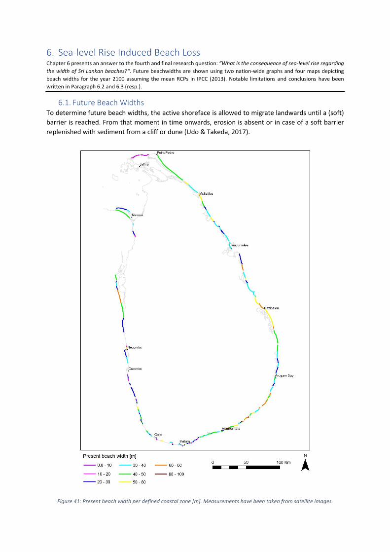
6. Sea-level Rise Induced Beach Loss Chapter 6 presents an answer to the fourth and final research question: ”What is the consequence of sea-level rise regarding
the width of Sri Lankan beaches?“. Future beachwidths are shown using two nation-wide graphs and four maps depicting
beach widths for the year 2100 assuming the mean RCPs in IPCC (2013). Notable limitations and conclusions have been
written in Paragraph 6.2 and 6.3 (resp.).
6.1. Future Beach Widths To determine future beach widths, the active shoreface is allowed to migrate landwards until a (soft)
barrier is reached. From that moment in time onwards, erosion is absent or in case of a soft barrier
replenished with sediment from a cliff or dune (Udo & Takeda, 2017).
Figure 41: Present beach width per defined coastal zone [m]. Measurements have been taken from satellite images.
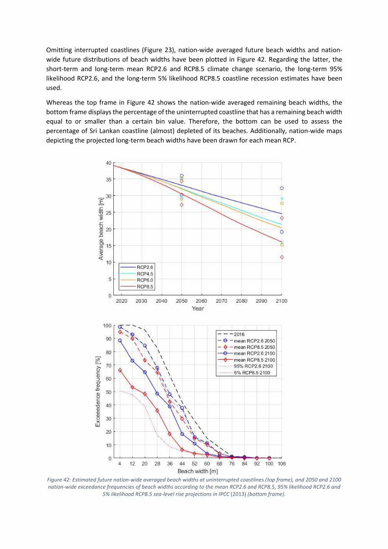
Omitting interrupted coastlines (Figure 23), nation-wide averaged future beach widths and nation-
wide future distributions of beach widths have been plotted in Figure 42. Regarding the latter, the
short-term and long-term mean RCP2.6 and RCP8.5 climate change scenario, the long-term 95%
likelihood RCP2.6, and the long-term 5% likelihood RCP8.5 coastline recession estimates have been
used.
Whereas the top frame in Figure 42 shows the nation-wide averaged remaining beach widths, the
bottom frame displays the percentage of the uninterrupted coastline that has a remaining beach width
equal to or smaller than a certain bin value. Therefore, the bottom can be used to assess the
percentage of Sri Lankan coastline (almost) depleted of its beaches. Additionally, nation-wide maps
depicting the projected long-term beach widths have been drawn for each mean RCP.
Figure 42: Estimated future nation-wide averaged beach widths at uninterrupted coastlines (top frame), and 2050 and 2100 nation-wide exceedance frequencies of beach widths according to the mean RCP2.6 and RCP8.5, 95% likelihood RCP2.6 and
5% likelihood RCP8.5 sea-level rise projections in IPCC (2013) (bottom frame).

Figure 43: Remaining 2100 beach widths along the Sri Lankan coast provided the mean RCP2.6 sea-level rise projections.

Figure 44: Remaining 2100 beach widths along the Sri Lankan coast provided the mean RCP4.5 sea-level rise projections.

Figure 45: Remaining 2100 beach widths along the Sri Lankan coast provided the mean RCP6.0 sea-level rise projections.

Figure 46: Remaining 2100 beach widths along the Sri Lankan coast provided the mean RCP8.5 sea-level rise projections.
6.2. Limitations Firstly, present beach widths have been measured using satellite images that are not guaranteed to
accurately provide the average position of the MSL mark of a cross-shore profile. Furthermore,
outlining present beaches is a tedious and ambiguous process often hindered by variying satellite
image qualities. Regions for which the image quality has been troublesome are the South-east coast,
the top half of the North-east coast and the Northern coastline. Beach width measurements have been
refined through multiple iterations, but remain prone to human error.
Secondly, depending on the landward barrier, the credibility of said barrier is high (dunes and built up
area) medium (permanent vegetation line) or low (backshore).
Thirdly, the results in Chapter 5 show the future position of interrupted coastlines is strongly
influenced by changes in the fluvial sediment supply of rivers, and/or coastal sediment import or
export by inlet-basin systems. The beaches downdrift from rivers and/or intermittently closed to
permanently open inlet-basin systems have been omitted in Paragraph 6.1. Consequently, the sandy
coastlines along the South and North-east of Sri Lanka are poorly represented.
6.3. Conclusions With the present landward limit to beaches locked in place, mean long-term sea-level rise will
considerably decrease beach widths at uninterrupted coastlines to a national average of 25 m (RCP2.6),
22 m (RCP4.5), 20 m (RCP6.0) or 16 m (RCP8.5).
Along the Northern coast, short-term sea-level rise is expected to reduce beach widths to zero. Long-
term sea-level rise and affiliated coastline recession may result in the disappearance of a considerable
amount of beaches along most of the Sri Lankan coast. Results show that diminishing beach widths are
not only limited to the more severe climate change scenarios. Long-term, the mean RCP2.6 climate
change scenario sea-level rise will result in depleted beaches along the North and parts of the West
coast of Sri Lanka as well.
7. General Conclusions Chapter 7 summarises the answers to the posed research question given in the previous chapters.
RQ 1: What is the validity of applying the Bruun rule in assessing the future position of the Sri Lankan
coastline?
The Bruun rule is a first-pass assessment of the coastline response to sea-level rise for approximately
half of the total Sri Lankan coast. However, diverenges in the littoral drift or cross-shore sources or
sinks influencing the coastal sediment balance cannot be precluded along respectively 78% and 51%
of the sandy coastline. Moreover, the presence of numerous (large) rivers, lagoons and/or coastal lakes
may result in deviations from the Bruun rule coastline recession estimates along 32% of the assessed
coast.
RQ 2: What is the predictive accuracy of the Bruun rule for the Sri Lankan coastline?
Bruun rule coastline recession estimates should be interpreted as the sea-level rise induced recession
of the average cross-shore location of the coastline. However, due to several limitations regarding the
performed Bruun rule hindcast (using the Satellite Derived Shoreline trends by Luijendijk et al. (2018))
and the comparison between Bruun rule coastline recession estimates and the Probabilistic Coastal
Recession method derived projections in Dastgheib et al. (2017), a clear answer to this research
question cannot be provided.
RQ 3: How far will the Sri Lankan coastline recede due to sea-level rise, and what influence have rivers
and inlet-basin systems?
On average, the mean long-term sea-level rise induced recession by the Sri Lankan coastline is 16 m,
21 m, 23 m or 31 m, depending on the imposed RCP. However, significant regional differences and
uncertainties in the coastline recession projections are present and should be taken into account.
The East and North-east lagoons are likely to result in mild to (dangerously) strong local coastline
recession trends. Along the Northern coast, inlet-basin systems within the Jaffna Peninsula are
expected result in local coastline progradation.
Climate change and continuing development of catchments will result in increased volumes of fluvial
sediments supplied to the Sri Lankan coast downdrift from mostly uncontrolled rivers. However, future
surpluses in supplied fluvial sediments may be nullified by increased river mining activities.
Consequently, strong local erosion trends at the beach adjacent to the Nilwala Ganga river mouth and
along the coastline downdrift from the Deduru Oya river mouth cannot be debarred.
RQ 4: What is the consequence of sea-level rise regarding the width of Sri Lankan beaches?
Provided the landward limit to present beaches is locked in place, long-term sea level rise may
significantly reduce the number of Sri Lankan beaches by the end of the 21st century. The mean RCP2.6
climate change scenario will result in diminished beachwidths limited to the North and parts of the
West coast of Sri Lanka. However, provided the mean RCP8.5 climate change scenario, the absence of
beaches will become a common phenomenon along most of the Sri Lankan coast.
8. Recommendations The following recommendation are proposed to mitigate the impact of future coastline recession, enrich the projection in
this report, and spark or help improvements and follow-up research linked to the used research method.
▪ Expecting mild to (dangerously) strong local erosion trends downdrift from the intermittently
closed and permanently opened inlet-basin systems along the East and North-east coast of Sri
Lanka, development of these coastlines should be discouraged or restricted to temporary
structures and infrastructure.
▪ Similarly, developments close to the coastline downdrift from the inlet of Chilaw lake and the
mouth of the Deduru Oya river are not adviseable.
▪ The landward limit to beaches must be allowed to migrate landwards where possible. The
West to South coast of Sri Lanka is heavily developed and unfortunately said landward
migration is often prohibited by property and infrastructure. Here nourishments of coastal
sediment balances may provide a solution.
▪ The Coast Conservation Department Sri Lanka is encouraged to continue the measuring of the
Sri Lankan coastline and increase the accuracy of the Bruun rule estimates. An important gap
in their present bathymetry measurements ensemble is between Galle and Tangalle. Figure 20
can be employed to identify other gaps.
▪ The Coast Conservation Department Sri Lanka is urged to collaborate with the Geological
Survey and Mining Bureau in determining present and future river mining activities in the
catchments of the Deduru Oya and Nilwala Ganga rivers, and downstream from large
reservoirs in the catchments of other rivers along the West to South-east coast.
▪ Originally this research aimed to include a (qualitative) analysis of sea-level rise related
economic damages. However, due to missing crucial information, it is not possible to present
a sufficiently complete overview of the following three dimensions to economic impact:
▪ loss of property expressed as either the value of property lost (Dastgheib et al., 2017)
or number of properties lost (Wadey et al., 2013);
▪ damage to roads and railways expressed as the length of infrastructure affected
(Wadey et al., 2013);
▪ devaluation of beach related ecosystem services such as recreation and tourism,
(commercial) fishery and amenity due to decreasing beach widths (Udo & Takeda,
2017) or beach surface area (Dastgheib et al., 2017).
Although the Sri Lankan coast is heavily developed and the potential damages to property and
infrastructure are considerable (Table 17), the comparison between the Bruun rule and the
Probabilistic Coastal Recession method in Paragraph 4.2 has shown that the use of the Bruun
rule (without the addition of interannual variability of storms) is not justifiable in an impact
analysis regarding these two dimensions. To include intra-annual variability in the position of
the shoreline, the approach by Toimil et al. (2017) and a the application of the Probabilistic
Coastal Recession method without sea-level rise are both options. However, in data poor
environments, scaling the Bruun rule (Table 17) may be the only option.
Alternative to the Openstreetmap database, the Global Urban Footprint by the German Earth
Observation Centre (or other satellite derived global urban area masks) can be used to
determine the amount of built up area lost. However, due to the poor performance of the
Global Urban Footprint in scarcely built up areas (Klotz et al., 2016; Mück et al, 2017), the
applicability of the Global Urban Footprint is limited to medium or high urban density areas.

Table 17: Presence of railways and connecting roads (categorised using the Openstreetmap highway key) [km], and permanent building polygons within 100 m of the MSL mark at unprotected sandy shorelines | enveloped by scaled Bruun rule coastline recession estimates at uninterrupted coastlines or explained by the SMIC method (Openstreetmap database).
Coastal sector Railways [km]
Roads [km] Buildings polygons Trunk Primary Secondary Tertiary
Southern
South-eastern
Eastern
North-eastern
Northern
North-western
Western
Southwestern
- |
- |
- |
- |
- |
≈ 0 | ≈ 0
27 | 1.3
2.1 | 0.8
6.9 | 1.1
- | -
0.8 | -
- | -
≈ 0 | 0.2
- | -
2.4 | 0.9
10 | 2.3
1.2 | 1.1
- | -
0.4 | -
- | -
2.4 | 1.9
1.1 | -
- | -
- | -
≈ 0 | -
0.3 | -
- | -
1.6 | 0.2
0.4 | ≈ 0
- | -
1.1 | -
≈ 0 | -
0.3 | ≈ 0
0.6 | -
5.2 | 7.1
6.2 | 1.0
- | -
- | -
5.8 | 0.4
0.3 | ≈ 0
793 | 195
48 | 2
514 | 325
1453 | 732
15 | 10
155 | 171
445 | 217
153 | 56
.
▪ Using the third generation Simulating Waves Nearshore model developed at Delft University
of Technology, offshore ERA-Interim reanalysed wave data (Dee et al., 2011) can be projected
onto a nearshore grid. The resulting refined nearshore wave conditions can be used to
estimate depth of closures more accurately. An example is found in Giardino et al. (2018).
▪ Alternative to the approach by Udo and Takeda (2017), the annual (nearshore) significant wave
heights exceeded for 12 hours and affiliated wave periods may be used to build two
generalised extreme value distributions. Said distributions can be used to determine the
required wave conditions exceeded for 12 hours at timescales within and outside that of the
employed (nearshore) wave data.
▪ Regarding the attenuation of the oceanic tide in large (with a wide inlet channel) inlet-basin
systems here a simplification assuming no tidal attenuation has been used . It is recommended
to either justify the simplication further or derive a new relation between the oceanic tide an
the tidal amplitude within the basin for (both small and) large inlet-basin systems. Provided
the aforementioned, the iterative approach by Bamunawala et al. (2018) is promising in
modelling present and future ebb tide flow volumes for both type I and type II inlet-basin
systems as it decreases the required variables to more easily observed variables such as inlet
channel length and width.
▪ An improved scaling of the Global Human Footprint Index for use in the BQART model may be
attained through the following steps:
1. Determine the catchment-wide GHFI value of each catchments used by Syvitski and
Milliman (2007) to derive the BQART model.
2. Average the catchment-wide GHFI values of the catchments associated with each Eh
class (Eh = 0.3, Eh = 1.0 or Eh = 2.0).
3. Fit a line through the three datapoints that allows Eh to be a function of the GHFI.
▪ To accurately incorporate river mining activities and increase the applicability of the BQART
model in other coastline recession studies a sound approach to combining the effects of
reservoir siltation and river mining activities should be sought.
▪ Future comparisons between the Bruun rule and the Probabilistic Coastal Recession method
is advised to use the annual average shoreline locations according to the Probabilisitc Coastal
Recession method with Bruun rule estimates and repeat the comparison for sandy coastlines
with different dimensions of the active shoreface.

References Argus, D. F., Peltier, W. R., Drummond, R., & Moore, A. W. (2014). The Antarctica component of postglacial rebound model
ICE-6G_C (VM5a) based on GPS positioning, exposure age dating of ice thicknesses, and relative sea level histories. Geophysical Journal International, 198(1), 537–563. https://doi.org/10.1093/gji/ggu140
Ballu, V., Bouin, M.-N., Simeoni, P., Crawford, W. C., Calmant, S., Bore, J.-M., … Pelletier, B. (2011). Comparing the role of absolute sea-level rise and vertical tectonic motions in coastal flooding, Torres Islands (Vanuatu). Proceedings of the National Academy of Sciences, 108(32), 13019–13022. https://doi.org/10.1073/pnas.1102842108
Bamunawala, J., Ranasinghe, R., van der Spek, A., Maskey, S., & Udo, K. (2018). Assessing Future Coastline Change in the Vicinity of Tidal Inlets. Journal of Coastal Research. https://doi.org/10.1007/s11947-009-0181-3
Brune, G. M. (1953). Trapping Efficiency of Reservoirs. American Geophysical Union, 34(3), 407–419.
Bruun, P. (1962). Sea Level Rise as a Form of Shore Erosion. Coastal and Ocean Engineering, 88(1), 117–130.
Camenen, B., & Larson, M. (2007). Predictive Formulas for Breaker Depth Index and Breaker Type. Journal of Coastal Research, 234(4), 1028–1041. https://doi.org/10.2112/05-0566.1
Castelle, B., & Coco, G. (2012). The morphodynamics of rip channels on embayed beaches. Continental Shelf Research, 43, 10–23. https://doi.org/10.1016/j.csr.2012.04.010
CCD. (2006). Coastal Zone Management Plan (CZMP) 2004. Gazette Extraordinary of the Democratic Socialist Republic of Sri Lanka. Retrieved from http://www.coastal.gov.lk/downloads/pdf/CZMP English.pdf
Cooper, J. A. G., & Pilkey, O. H. (2004). Sea-level rise and shoreline retreat: Time to abandon the Bruun Rule. Global and Planetary Change, 43(3–4), 157–171. https://doi.org/10.1016/j.gloplacha.2004.07.001
Cowell, P. J., Stive, M. J. F., Niedoroda, A. W., Swift, D. J. P., De Vriend, H. J., Buijsman, M. C., … De Boer, P. L. (2003). The coastal-tract (part 2): Applications of aggregated modeling of low-order coastal change. Journal of Coastal Research, 19(4), 828–848. https://doi.org/10.2112%2F0749-0208%282003%29019%5B0828%3ATCPAOA%5D2.3.CO%3B2
Cowell, P. J., Thom, B. G., Jones, R. A., Everts, C. H., & Simanovic, D. (2006). Management of Uncertainty in Predicting Climate-Change Impacts on Beaches. Journal of Coastal Research, 221, 232–245. https://doi.org/10.2112/05A-0018.1
Da Cruz, C. M. (2018). Stochastic Projections of Coastline Variations: Application to Hasaki Beach, Japan. IHE-Delft Institute for Water Education.
Dastgheib, A., Jongejan, R., Mehvar, S. A., & Ranasinghe, R. (2017). Coastal Risk Assessment Along the East Coast of Sri Lanka.
Dayananda, H. V. (1992). Shoreline Erosion in Sri Lanka’s Coastal Areas.
Dean, R. G. (1991). Equilibrium Beach Profiles : Characteristics and Applications. Journal of Coastal Research, 7(1), 53–84. Retrieved from http://www.jstor.org/stable/4297805
Dean, R. G. (1995). Cross-shore sediment transport processes. Coastal Engineering Manual, 1, 152–...
Dean, R. G., & Dalrymple, R. A. (2001). Coastal processes with engineering applications (2004th ed.). Cambridge: Cambridge University Press. Retrieved from http://marineman.ir/wp-content/uploads/2015/03/Coastal_Processes_with_Engineering_Applications__Cambridge_Ocean_Technology_Series_.pdf?v=d6392e39ad2a
Dee, D. P., Uppala, S. M., Simmons, A. J., Berrisford, P., Poli, P., Kobayashi, S., … Vitart, F. (2011). The ERA-Interim reanalysis: Configuration and performance of the data assimilation system. Quarterly Journal of the Royal Meteorological Society, 137(656), 553–597. https://doi.org/10.1002/qj.828
Department of Irrigation Sri Lanka. (2018). Online Reservoir Status. Retrieved March 16, 2018, from http://www.irrigation.gov.lk/index.php?option=com_gmapfp&view=gmapfp&layout=categorie&catid=124&id_perso=0&Itemid=221&lang=en
Department of Meteorology Sri Lanka. (2016). Climate of Sri Lanka. Retrieved April 4, 2018, from http://www.meteo.gov.lk/index.php?option=com_content&view=article&id=94&Itemid=310&lang=en
Duong, T. M. (2015). Climate Change Impacts on the Stability of Small Tidal Inlets.
Duong, T. M., Ranasinghe, R., Walstra, D., & Roelvink, D. (2016). Assessing climate change impacts on the stability of small tidal inlet systems: Why and how? Earth-Science Reviews, 154, 369–380.
https://doi.org/10.1016/j.earscirev.2015.12.001
Edelman, T. (1976). Dune erosion during storm surge conditions. Hydro Delft, 45, Dec., 2–3. https://doi.org/10.9753/icce.v13.%25p
Engle, V. D., Kurtz, J. C., Smith, L. M., Chancy, C., & Bourgeois, P. (2007). A classification of U.S. estuaries based on physical and hydrologic attributes. Environmental Monitoring and Assessment, 129(1–3), 397–412. https://doi.org/10.1007/s10661-006-9372-9
Giardino, A., Schrijvershof, R., Nederhoff, C. M., de Vroeg, H., Brière, C., Tonnon, P. K., … Sloff, C. J. (2018). A quantitative assessment of human interventions and climate change on the West African sediment budget. Ocean and Coastal Management, 156, 249–265. https://doi.org/10.1016/j.ocecoaman.2017.11.008
Global Energy Observatorium. (2018). No Title. Retrieved March 16, 2018, from http://globalenergyobservatory.org/select.php?tgl=Edit
Hallermeier, R. J. (1980). A profile zonation for seasonal sand beaches from wave climate. Coastal Engineering, 4(C), 253–277. https://doi.org/10.1016/0378-3839(80)90022-8
Heinemarm, H. G. (1981). a New Sediment Trap Efficiency Curve for Small Reservoirs. JAWRA Journal of the American Water Resources Association, 17(5), 825–830. https://doi.org/10.1111/j.1752-1688.1981.tb01304.x
IHE-Delft. (2016). Delft3D model based alongshore sediment transport rates at Pesalai , Gurunagar , Point Pedro and Mullaitivu , Sri Lanka (Phase 2 Final Report). Delft.
IPCC. (2013). Climate Change 2013: The Physical Science Basis. New York. https://doi.org/10.1017/CB09781107415315.026
Jacobsen, P. R., Perera, N., & Jensen, K. B. (1987). Master Plan for Coastal Erosion Management. Retrieved from https://www.researchgate.net/publication/294306230_Master_plan_for_coast_erosion_management
Jarvis, A., Reuter, H. I., Nelson, A., & Guevara, E. (2008). Hole-filled SRTM for the globe Version 4, International Centre for Tropical Agriculture (CIAT), Available at: http://srtm.csi.cgiar.org.
Jayasekera, D. L., Kaluarachchi, J. J., & Villholth, K. G. (2011). Groundwater stress and vulnerability in rural coastal aquifers under competing demands: A case study from Sri Lanka. Environmental Monitoring and Assessment, 176(1–4), 13–30. https://doi.org/10.1007/s10661-010-1563-8
Jayathilaka, R. M. R. M. (2015). Large Scale Sediment Budgets in Data Poor Environments via Numerical Modelling. UNESCO-IHE Institute for Water Education.
Jayawardena, U. de S., & Sarathchandra, M. J. (1995). Land subsidence and other environmental impacts due to groundwater extraction from fractured hard rocks in Sri Lanka. Land Subsidence (Fifth International Symposium of Land Subsidence), (234), 439–444.
Jiménez, J. A., Sánchez-Arcilla, A., & Stive, J. F. (1993). Prediction of Storm Normal Beach Profiles. Journal of Waterway Port Coastal and Ocean Engineering.
Keulegan, G. H. (1967). Tidal Flow in Entrances; Water-Level Fluctuations of Basins in Communication With Seas.
Klotz, M., Kemper, T., Geiß, C., Esch, T., & Taubenböck, H. (2016). How good is the map? A multi-scale cross-comparison framework for global settlement layers: Evidence from Central Europe. Remote Sensing of Environment, 178, 191–212. https://doi.org/10.1016/j.rse.2016.03.001
Komar, P. D. (1983). CRC Handbook of Coastal Processes and Erosion. Boca Raton: CRC Press.
Kummu, M., Lu, X. X., Wang, J. J., & Varis, O. (2010). Basin-wide sediment trapping efficiency of emerging reservoirs along the Mekong. Geomorphology, 119(3–4), 181–197. https://doi.org/10.1016/j.geomorph.2010.03.018
Larson, M., Erikson, L., & Hanson, H. (2004). An analytical model to predict dune erosion due to wave impact. Coastal Engineering, 51(8–9), 675–696. https://doi.org/10.1016/j.coastaleng.2004.07.003
Le Cozannet, G., Oliveros, C., Castelle, B., Garcin, M., Idier, D., Pedreros, R., & Rohmer, J. (2016). Uncertainties in Sandy Shorelines Evolution under the Bruun Rule Assumption. Frontiers in Marine Science, 3, 49. https://doi.org/10.3389/fmars.2016.00049
Luijendijk, A., Hagenaars, G., Ranasinghe, R., Baart, F., Donchyts, G., & Aarninkhof, S. (2018). The State of the World’s Beaches. Nature Scientific Reports, 8, 1–11. https://doi.org/10.1038/s41598-018-24630-6
McCarroll, R. J., Brander, R. W., MacMahan, J. H., Turner, I. L., Reniers, A. J. H. M., Brown, J. A., … Sherker, S. (2014).
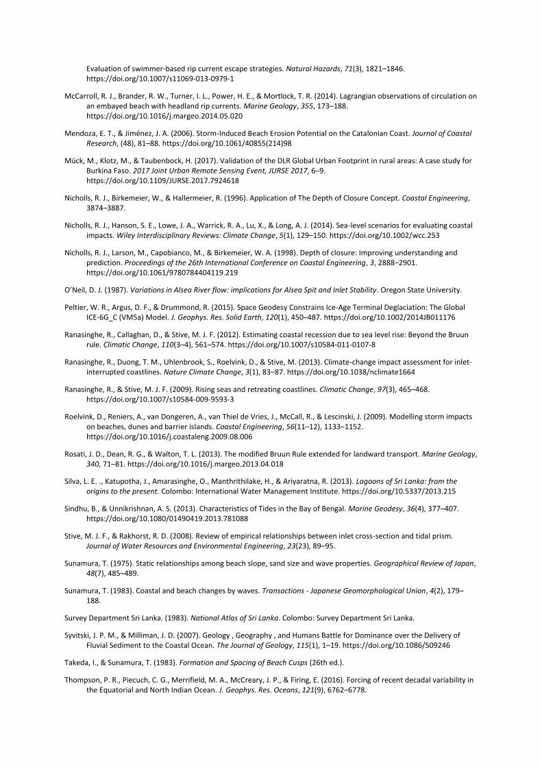
Evaluation of swimmer-based rip current escape strategies. Natural Hazards, 71(3), 1821–1846. https://doi.org/10.1007/s11069-013-0979-1
McCarroll, R. J., Brander, R. W., Turner, I. L., Power, H. E., & Mortlock, T. R. (2014). Lagrangian observations of circulation on an embayed beach with headland rip currents. Marine Geology, 355, 173–188. https://doi.org/10.1016/j.margeo.2014.05.020
Mendoza, E. T., & Jiménez, J. A. (2006). Storm-Induced Beach Erosion Potential on the Catalonian Coast. Journal of Coastal Research, (48), 81–88. https://doi.org/10.1061/40855(214)98
Mück, M., Klotz, M., & Taubenbock, H. (2017). Validation of the DLR Global Urban Footprint in rural areas: A case study for Burkina Faso. 2017 Joint Urban Remote Sensing Event, JURSE 2017, 6–9. https://doi.org/10.1109/JURSE.2017.7924618
Nicholls, R. J., Birkemeier, W., & Hallermeier, R. (1996). Application of The Depth of Closure Concept. Coastal Engineering, 3874–3887.
Nicholls, R. J., Hanson, S. E., Lowe, J. A., Warrick, R. A., Lu, X., & Long, A. J. (2014). Sea-level scenarios for evaluating coastal impacts. Wiley Interdisciplinary Reviews: Climate Change, 5(1), 129–150. https://doi.org/10.1002/wcc.253
Nicholls, R. J., Larson, M., Capobianco, M., & Birkemeier, W. A. (1998). Depth of closure: Improving understanding and prediction. Proceedings of the 26th International Conference on Coastal Engineering, 3, 2888–2901. https://doi.org/10.1061/9780784404119.219
O’Neil, D. J. (1987). Variations in Alsea River flow: implications for Alsea Spit and Inlet Stability. Oregon State University.
Peltier, W. R., Argus, D. F., & Drummond, R. (2015). Space Geodesy Constrains Ice-Age Terminal Deglaciation: The Global ICE-6G_C (VM5a) Model. J. Geophys. Res. Solid Earth, 120(1), 450–487. https://doi.org/10.1002/2014JB011176
Ranasinghe, R., Callaghan, D., & Stive, M. J. F. (2012). Estimating coastal recession due to sea level rise: Beyond the Bruun rule. Climatic Change, 110(3–4), 561–574. https://doi.org/10.1007/s10584-011-0107-8
Ranasinghe, R., Duong, T. M., Uhlenbrook, S., Roelvink, D., & Stive, M. (2013). Climate-change impact assessment for inlet-interrupted coastlines. Nature Climate Change, 3(1), 83–87. https://doi.org/10.1038/nclimate1664
Ranasinghe, R., & Stive, M. J. F. (2009). Rising seas and retreating coastlines. Climatic Change, 97(3), 465–468. https://doi.org/10.1007/s10584-009-9593-3
Roelvink, D., Reniers, A., van Dongeren, A., van Thiel de Vries, J., McCall, R., & Lescinski, J. (2009). Modelling storm impacts on beaches, dunes and barrier islands. Coastal Engineering, 56(11–12), 1133–1152. https://doi.org/10.1016/j.coastaleng.2009.08.006
Rosati, J. D., Dean, R. G., & Walton, T. L. (2013). The modified Bruun Rule extended for landward transport. Marine Geology, 340, 71–81. https://doi.org/10.1016/j.margeo.2013.04.018
Silva, L. E. ., Katupotha, J., Amarasinghe, O., Manthrithilake, H., & Ariyaratna, R. (2013). Lagoons of Sri Lanka: from the origins to the present. Colombo: International Water Management Institute. https://doi.org/10.5337/2013.215
Sindhu, B., & Unnikrishnan, A. S. (2013). Characteristics of Tides in the Bay of Bengal. Marine Geodesy, 36(4), 377–407. https://doi.org/10.1080/01490419.2013.781088
Stive, M. J. F., & Rakhorst, R. D. (2008). Review of empirical relationships between inlet cross-section and tidal prism. Journal of Water Resources and Environmental Engineering, 23(23), 89–95.
Sunamura, T. (1975). Static relationships among beach slope, sand size and wave properties. Geographical Review of Japan, 48(7), 485–489.
Sunamura, T. (1983). Coastal and beach changes by waves. Transactions - Japanese Geomorphological Union, 4(2), 179–188.
Survey Department Sri Lanka. (1983). National Atlas of Sri Lanka. Colombo: Survey Department Sri Lanka.
Syvitski, J. P. M., & Milliman, J. D. (2007). Geology , Geography , and Humans Battle for Dominance over the Delivery of Fluvial Sediment to the Coastal Ocean. The Journal of Geology, 115(1), 1–19. https://doi.org/10.1086/509246
Takeda, I., & Sunamura, T. (1983). Formation and Spacing of Beach Cusps (26th ed.).
Thompson, P. R., Piecuch, C. G., Merrifield, M. A., McCreary, J. P., & Firing, E. (2016). Forcing of recent decadal variability in the Equatorial and North Indian Ocean. J. Geophys. Res. Oceans, 121(9), 6762–6778.

https://doi.org/10.1002/2016JC012132
Toimil, A., Losada, I. J., Camus, P., & Díaz-Simal, P. (2017). Managing coastal erosion under climate change at the regional scale. Coastal Engineering, 128(November 2016), 106–122. https://doi.org/10.1016/j.coastaleng.2017.08.004
Udo, K., & Takeda, Y. (2017). Projections of Future Beach Loss in Japan Due to Sea-Level Rise and Uncertainties in Projected Beach Loss. Coastal Engineering Journal, 59(02), 1740006. https://doi.org/10.1142/S057856341740006X
Velegrakis, F., & Schimmels, S. (2013). Predicting Beach Face rotation on a Meso Tidal, Steeply Sloping Beach. Coastal Dynamics, 1835–1846.
Verstraeten, G., & Poesen, J. (2000). Estimating trap efficiency of small reservoirs and ponds: methods and implications for the assessment of sediment yield. Progress in Physical Geography, 24(2), 219–251. https://doi.org/10.1177/030913330002400204
Vörösmarty, C. J., Meybeck, M., Fekete, B., Sharma, K., Green, P., & Syvitski, J. P. M. (2003). Anthropogenic sediment retention: Major global impact from registered river impoundments. Global and Planetary Change, 39(1–2), 169–190. https://doi.org/10.1016/S0921-8181(03)00023-7
Wadey, M. P., Roberts, H., & Harris, J. (2013). Impacts of climate change on built structures (onshore and coastal). Marine Climate Change Impacts Partnership Science Review, 284–294. https://doi.org/10.14465
Wickramaarachchi, B. (2010). Spatial Analysis & Mapping, Maha Oya Low Land Corridor.
Wickramagamage, P., Wickramanayake, N., Kumarihamy, K., Vidanapathirana, E., & Larson, M. (2012). A comparative study of elevation data from different sources for mapping the coastal inlets and their catchment boundaries. Journal of the National Science Foundation of Sri Lanka, 40(1), 55–65. https://doi.org/10.4038/jnsfsr.v40i1.4169
Wijeratne, E. M. S. (n.d.). Sea Level Measurements and Coastal Ocean Modelling in Sri Lanka.
Wijeratne, E. M. S., & Pattiaratchi, C. B. (2017). Sea Level Variability in Sri Lanka Waters. Retrieved from http://wcrp.ipsl.jussieu.fr/Workshops/SeaLevel/Posters/2_1_WijeratneRevised.pdf
Wildlife Conservation Society - WCS and Center for International Earth Science Information Network - CIESIN - Columbia. (2005). Last of the Wild Project, Version 2, 2005 (LWP-2): Last of the Wild Dataset.
Zhang, K., Douglas, B. C., & Leatherman, S. P. (2004). Global warming and coastal erosion. Climatic Change, 64(1–2), 41–58. https://doi.org/10.1023/B:CLIM.0000024690.32682.48
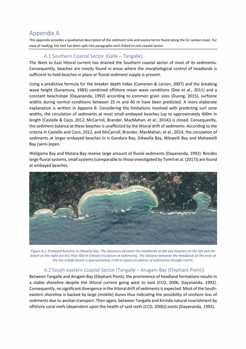
Appendix A This appendix provides a qualitative description of the sediment sink and source terms found along the Sri Lankan coast. For
ease of reading, the text has been split into paragraphs each linked to one coastal sector.
A.1 Southern Coastal Sector (Galle – Tangalle) The West to East littoral current has drained the Southern coastal sector of most of its sediments.
Consequently, beaches are mostly found in areas where the morphological control of headlands is
sufficient to hold beaches in place or fluvial sediment supply is present.
Using a predictive formula for the breaker depth index (Camenen & Larson, 2007) and the breaking
wave height (Sunamura, 1983) combined offshore mean wave conditions (Dee et al., 2011) and a
constant beachslope (Dayananda, 1992) according to common grain sizes (Duong, 2015), surfzone
widths during normal conditions between 25 m and 40 m have been predicted. A more elaborate
explanation is written in Appenix B. Considering the limitations involved with predicting surf zone
widths, the circulation of sediments at most small embayed beaches (up to approximately 400m in
length (Castelle & Coco, 2012; McCarroll, Brander, MacMahan, et al., 2014)) is closed. Consequenlty,
the sediment balance at these beaches is unaffected by the littoral drift of sediments. According to the
criteria in Castelle and Coco, 2012, and McCarroll, Brander, MacMahan, et al., 2014, the circulation of
sediments at larger embayed beaches in is Gandura Bay, Dikwella Bay, Nilewelli Bay and Mahawelli
Bay (semi-)open.
Weligama Bay and Matara Bay receive large amount of fluvial sediments (Dayananda, 1992). Besides
large fluvial systems, small systems (comparable to those investigated by Toimil et al. (2017)) are found
at embayed beaches.
Figure A.1: Embayed beaches in Dikwella Bay. The distances between the headlands at the two beaches on the left and the beach on the right are less than 400 m (closed circulation of sediments). The distance between the headlands at the ends of
the the middle beach is approximately 1100 m (open circulation of sediments) (Google Earth).
A.2 South-eastern Coastal Sector (Tangalle – Arugam Bay (Elephant Point)) Between Tangalle and Arugam Bay (Elephant Point), the prominence of headland formations results in
a stable shoreline despite the littoral current going west to east (CCD, 2006; Dayananda, 1992).
Consequently, no significant divergence in the littoral drift of sediments is expected. Most of the South-
eastern shoreline is backed by large (mobile) dunes thus indicating the possibility of onshore loss of
sediments due to aeolian transport. Then again, between Tangalle and Kirinda natural nourishment by
offshore coral reefs (dependent upon the health of said reefs (CCD, 2006)) exists (Dayananda, 1992).
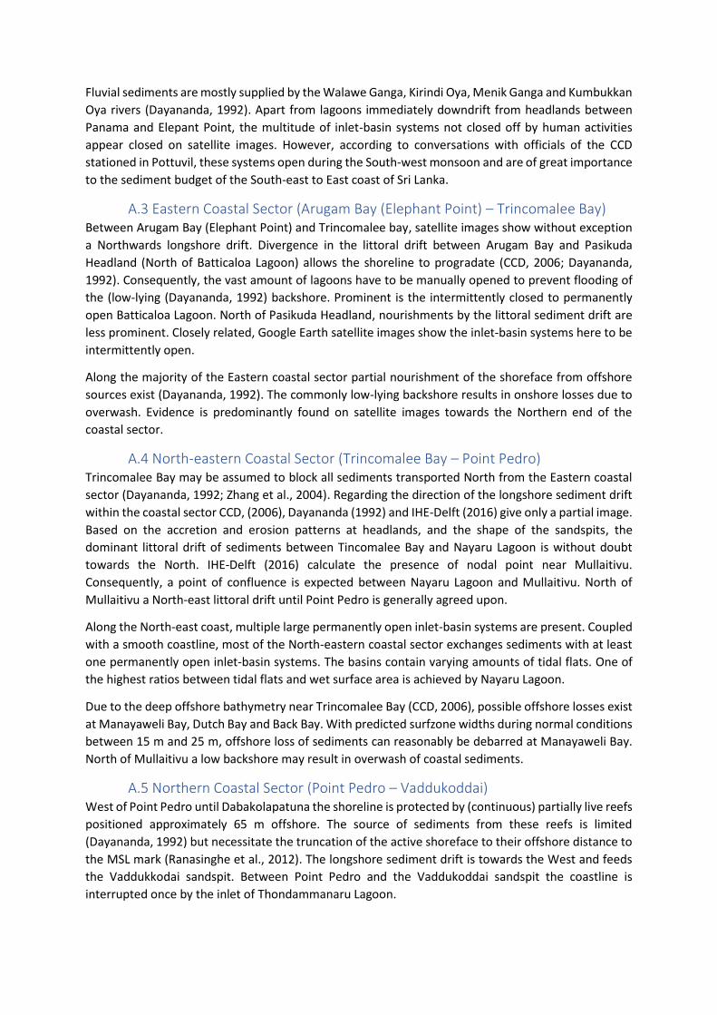
Fluvial sediments are mostly supplied by the Walawe Ganga, Kirindi Oya, Menik Ganga and Kumbukkan
Oya rivers (Dayananda, 1992). Apart from lagoons immediately downdrift from headlands between
Panama and Elepant Point, the multitude of inlet-basin systems not closed off by human activities
appear closed on satellite images. However, according to conversations with officials of the CCD
stationed in Pottuvil, these systems open during the South-west monsoon and are of great importance
to the sediment budget of the South-east to East coast of Sri Lanka.
A.3 Eastern Coastal Sector (Arugam Bay (Elephant Point) – Trincomalee Bay) Between Arugam Bay (Elephant Point) and Trincomalee bay, satellite images show without exception
a Northwards longshore drift. Divergence in the littoral drift between Arugam Bay and Pasikuda
Headland (North of Batticaloa Lagoon) allows the shoreline to progradate (CCD, 2006; Dayananda,
1992). Consequently, the vast amount of lagoons have to be manually opened to prevent flooding of
the (low-lying (Dayananda, 1992) backshore. Prominent is the intermittently closed to permanently
open Batticaloa Lagoon. North of Pasikuda Headland, nourishments by the littoral sediment drift are
less prominent. Closely related, Google Earth satellite images show the inlet-basin systems here to be
intermittently open.
Along the majority of the Eastern coastal sector partial nourishment of the shoreface from offshore
sources exist (Dayananda, 1992). The commonly low-lying backshore results in onshore losses due to
overwash. Evidence is predominantly found on satellite images towards the Northern end of the
coastal sector.
A.4 North-eastern Coastal Sector (Trincomalee Bay – Point Pedro) Trincomalee Bay may be assumed to block all sediments transported North from the Eastern coastal
sector (Dayananda, 1992; Zhang et al., 2004). Regarding the direction of the longshore sediment drift
within the coastal sector CCD, (2006), Dayananda (1992) and IHE-Delft (2016) give only a partial image.
Based on the accretion and erosion patterns at headlands, and the shape of the sandspits, the
dominant littoral drift of sediments between Tincomalee Bay and Nayaru Lagoon is without doubt
towards the North. IHE-Delft (2016) calculate the presence of nodal point near Mullaitivu.
Consequently, a point of confluence is expected between Nayaru Lagoon and Mullaitivu. North of
Mullaitivu a North-east littoral drift until Point Pedro is generally agreed upon.
Along the North-east coast, multiple large permanently open inlet-basin systems are present. Coupled
with a smooth coastline, most of the North-eastern coastal sector exchanges sediments with at least
one permanently open inlet-basin systems. The basins contain varying amounts of tidal flats. One of
the highest ratios between tidal flats and wet surface area is achieved by Nayaru Lagoon.
Due to the deep offshore bathymetry near Trincomalee Bay (CCD, 2006), possible offshore losses exist
at Manayaweli Bay, Dutch Bay and Back Bay. With predicted surfzone widths during normal conditions
between 15 m and 25 m, offshore loss of sediments can reasonably be debarred at Manayaweli Bay.
North of Mullaitivu a low backshore may result in overwash of coastal sediments.
A.5 Northern Coastal Sector (Point Pedro – Vaddukoddai) West of Point Pedro until Dabakolapatuna the shoreline is protected by (continuous) partially live reefs
positioned approximately 65 m offshore. The source of sediments from these reefs is limited
(Dayananda, 1992) but necessitate the truncation of the active shoreface to their offshore distance to
the MSL mark (Ranasinghe et al., 2012). The longshore sediment drift is towards the West and feeds
the Vaddukkodai sandspit. Between Point Pedro and the Vaddukoddai sandspit the coastline is
interrupted once by the inlet of Thondammanaru Lagoon.
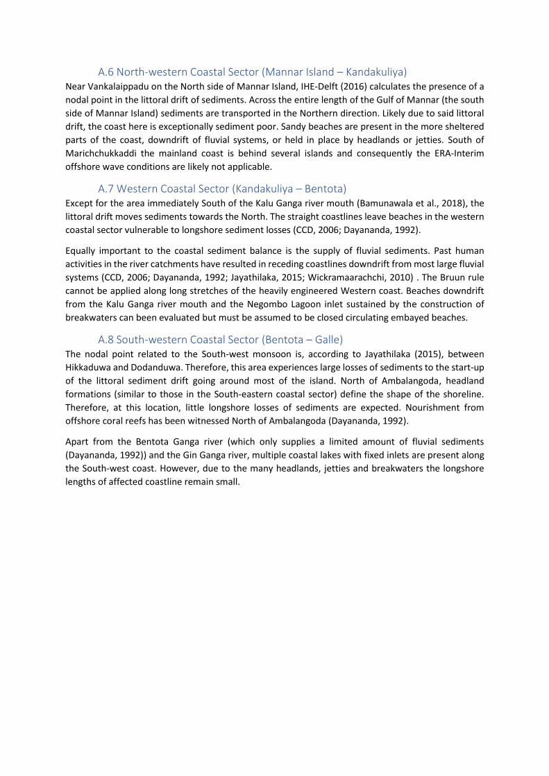
A.6 North-western Coastal Sector (Mannar Island – Kandakuliya) Near Vankalaippadu on the North side of Mannar Island, IHE-Delft (2016) calculates the presence of a
nodal point in the littoral drift of sediments. Across the entire length of the Gulf of Mannar (the south
side of Mannar Island) sediments are transported in the Northern direction. Likely due to said littoral
drift, the coast here is exceptionally sediment poor. Sandy beaches are present in the more sheltered
parts of the coast, downdrift of fluvial systems, or held in place by headlands or jetties. South of
Marichchukkaddi the mainland coast is behind several islands and consequently the ERA-Interim
offshore wave conditions are likely not applicable.
A.7 Western Coastal Sector (Kandakuliya – Bentota) Except for the area immediately South of the Kalu Ganga river mouth (Bamunawala et al., 2018), the
littoral drift moves sediments towards the North. The straight coastlines leave beaches in the western
coastal sector vulnerable to longshore sediment losses (CCD, 2006; Dayananda, 1992).
Equally important to the coastal sediment balance is the supply of fluvial sediments. Past human
activities in the river catchments have resulted in receding coastlines downdrift from most large fluvial
systems (CCD, 2006; Dayananda, 1992; Jayathilaka, 2015; Wickramaarachchi, 2010) . The Bruun rule
cannot be applied along long stretches of the heavily engineered Western coast. Beaches downdrift
from the Kalu Ganga river mouth and the Negombo Lagoon inlet sustained by the construction of
breakwaters can been evaluated but must be assumed to be closed circulating embayed beaches.
A.8 South-western Coastal Sector (Bentota – Galle) The nodal point related to the South-west monsoon is, according to Jayathilaka (2015), between
Hikkaduwa and Dodanduwa. Therefore, this area experiences large losses of sediments to the start-up
of the littoral sediment drift going around most of the island. North of Ambalangoda, headland
formations (similar to those in the South-eastern coastal sector) define the shape of the shoreline.
Therefore, at this location, little longshore losses of sediments are expected. Nourishment from
offshore coral reefs has been witnessed North of Ambalangoda (Dayananda, 1992).
Apart from the Bentota Ganga river (which only supplies a limited amount of fluvial sediments
(Dayananda, 1992)) and the Gin Ganga river, multiple coastal lakes with fixed inlets are present along
the South-west coast. However, due to the many headlands, jetties and breakwaters the longshore
lengths of affected coastline remain small.
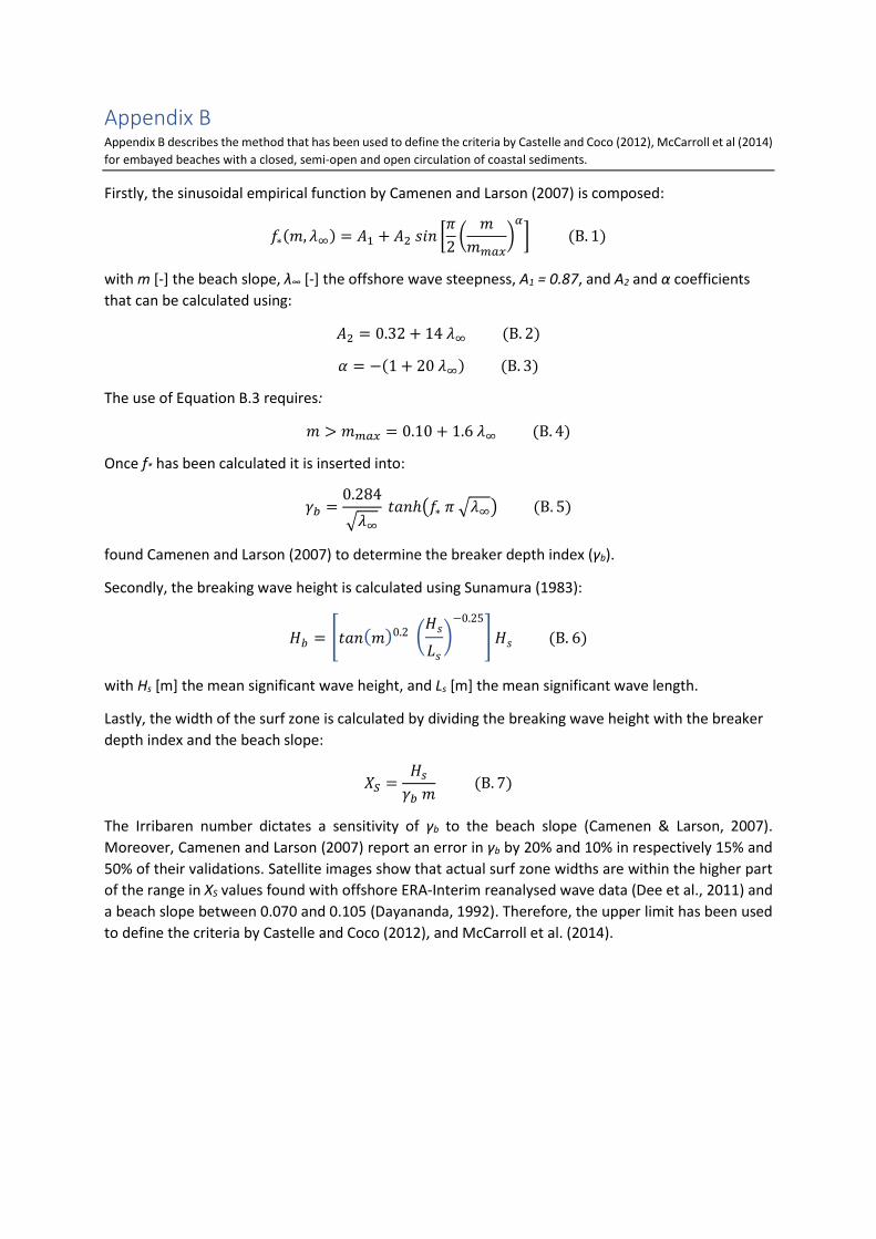
Appendix B Appendix B describes the method that has been used to define the criteria by Castelle and Coco (2012), McCarroll et al (2014)
for embayed beaches with a closed, semi-open and open circulation of coastal sediments.
Firstly, the sinusoidal empirical function by Camenen and Larson (2007) is composed:
𝑓∗(𝑚, 𝜆∞) = 𝐴1 + 𝐴2 𝑠𝑖𝑛 [𝜋
2(
𝑚
𝑚𝑚𝑎𝑥)
𝛼
] (B. 1)
with m [-] the beach slope, λ∞ [-] the offshore wave steepness, A1 = 0.87, and A2 and α coefficients
that can be calculated using:
𝐴2 = 0.32 + 14 𝜆∞ (B. 2)
𝛼 = −(1 + 20 𝜆∞) (B. 3)
The use of Equation B.3 requires:
𝑚 > 𝑚𝑚𝑎𝑥 = 0.10 + 1.6 𝜆∞ (B. 4)
Once f* has been calculated it is inserted into:
𝛾𝑏 =0.284
√𝜆∞
𝑡𝑎𝑛ℎ(𝑓∗ 𝜋 √𝜆∞) (B. 5)
found Camenen and Larson (2007) to determine the breaker depth index (γb).
Secondly, the breaking wave height is calculated using Sunamura (1983):
𝐻𝑏 = [𝑡𝑎𝑛(𝑚)0.2 (𝐻𝑠
𝐿𝑠
)−0.25
] 𝐻𝑠 (B. 6)
with Hs [m] the mean significant wave height, and Ls [m] the mean significant wave length.
Lastly, the width of the surf zone is calculated by dividing the breaking wave height with the breaker
depth index and the beach slope:
𝑋𝑆 =𝐻𝑠
𝛾𝑏 𝑚 (B. 7)
The Irribaren number dictates a sensitivity of γb to the beach slope (Camenen & Larson, 2007).
Moreover, Camenen and Larson (2007) report an error in γb by 20% and 10% in respectively 15% and
50% of their validations. Satellite images show that actual surf zone widths are within the higher part
of the range in XS values found with offshore ERA-Interim reanalysed wave data (Dee et al., 2011) and
a beach slope between 0.070 and 0.105 (Dayananda, 1992). Therefore, the upper limit has been used
to define the criteria by Castelle and Coco (2012), and McCarroll et al. (2014).

Appendix C Future shortages in fluvial sediments supplied to the coast by rivers and volumes of coastal sediments imported by inlet-basin
systems.
Deduru Oya
Kelani Ganga
Kalu Ganga
Ging Ganga
Nilwala Ganga
Walawe Ganga
Kirindi Oya
Menik Ganga
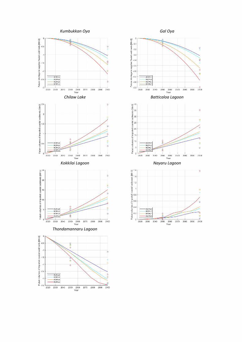
Kumbukkan Oya
Gal Oya
Chilaw Lake
Batticaloa Lagoon
Kokkilai Lagoon
Nayaru Lagoon
Thondamannaru Lagoon
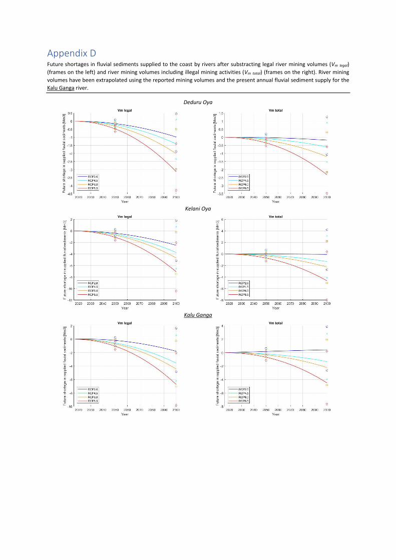
Appendix D Future shortages in fluvial sediments supplied to the coast by rivers after substracting legal river mining volumes (Vm legal)
(frames on the left) and river mining volumes including illegal mining activities (Vm total) (frames on the right). River mining
volumes have been extrapolated using the reported mining volumes and the present annual fluvial sediment supply for the
Kalu Ganga river.
Deduru Oya
Kelani Oya
Kalu Ganga

Gin Ganga
Nilwala Ganga
Menik Ganga
Kumbukkan Oya