fundamental of pid control - pdhonline.com · fundamental of pid control anthony k. ho ... fairfax,...

An Approved Continuing Education Provider

PDHonline Course E331 (3 PDH)

Fundamental of PID Control

Anthony K. Ho, P.E.

2014

PDH Online | PDH Center

5272 Meadow Estates Drive

Fairfax, VA 22030-6658

Phone & Fax: 703-988-0088

www.PDHonline.org

www.PDHcenter.com

http://www.pdhonline.org/

http://www.pdhcenter.com/

www.PDHcenter.com PDHonline Course E331 www.PDHonline.org

Table of Content

1. History and Background of PID Control ............................................................. 1

2. Theory of PID Control ......................................................................................... 2

2.1. Proportional Control .................................................................................. 3

2.2. Integral Control ......................................................................................... 5

2.3. Derivative Control ..................................................................................... 6

3. Implementation of PID Control ........................................................................... 9

3.1. Choosing the structure of a PID controller ............................................... 9

3.2. Tuning the PID controller .......................................................................11

4. Open-loop vs. Closed-loop Control ...................................................................13

5. Example - PID Controller for DC Motor ...........................................................14

6. Cascade Control .................................................................................................17

7. Troubleshooting PID Control ............................................................................19




©2014 Anthony K. Ho Page 1 of 20

1. History and Background of PID Control

The original technology for industrial proportional, integral, and derivative (PID)

control was pneumatic, hydraulic, or mechanical and the controller usually had a

simple interface for manual tuning. The first theoretical analysis of a PID

controller dates back to 1922 when the Russian American engineer Nicolas

Minorsky developed an automatic ship steering system for the U.S. Navy based on

observations of the steersmen’s use of current error, past error, and rate of change

to keep the ship on course. Controllers with electrical systems were developed

after World War II.

PID control is used to control and maintain processes. It can be used to control

physical variables such as temperature, pressure, flow rate, and tank level. The

technique is widely used in today’s manufacturing industry to achieve accurate

process control under different process conditions. PID is simply an equation that

the controller uses to evaluate the controlled variables. A process variable (PV)

temperature, for example, is measured, and a feedback signal is sent to the

controller. The controller then compares the feedback signal to the set point (SP)

and generates an error value. The value is examined with one or more of the three

proportional, integral, and derivative methodologies. As a result, the controller

issues the necessary commands or alters the control variable (CV) to correct the

error (E). These procedures form an iterative process. Below is a common control

loop application.

In this example, oil is flowing into the tank in a non-constant rate. The oil level in

the tank is the process variable, which is measured, and this information is fed

back to the controller. An operator enters a set point for a desired level. The

controller compares the current level with the set point and generates a value that is





examined with a PID method. The controller then adjusts the valve position to

correct the error.

2. Theory of PID Control

PID controllers typically use control loop feedback in industrial and control

systems applications. The controller first computes a value of error as the

difference between a measured process variable and a preferred set point. It then

tries to minimize the error by increasing or decreasing the control inputs or outputs

in the process so that the process variable moves closer to the set point. This

method is most useful when a mathematical model of the process or control is too

complicated or unknown for the system. To increase performance, such as by

increasing the system’s responsiveness, PID parameters must be adjusted

according to the specific application.

The block diagram below shows an example of a heating process that is controlled

by a PID controller (programmable logic controller or PLC in this case). The

temperature of the furnace is controlled by adjusting the gas valve. The operator

sets the desired temperature as the set point. The furnace’s temperature is

measured, and this information is sent back to the controller. The feedback is

compared to the set point, and an error value is calculated. The PID equations then

determine the suitable valve position to correct the error. In fact, this is an example

of a PID feedback control loop.

The following figure shows a typical step response curve after a controller

responds to a set point change. The curve rises from 10% to 90% of final steady





state value within a period known as the rise time. The curve rises from 0% to

63.2% of peak value within a period known as the step response time. The rise

time is equal to the step response time minus the dead time.

One of the advantages of PID is that for many processes there are straightforward

correlations between the process responses and the use and tuning of the three

terms (P, I, and D) by the controller. Designing a PID system involves two steps.

First, the engineer must choose the structure of the PID controller, for example P

only, P and I, or all three terms P, I, and D. Second, to tune the controller, the

engineer must choose numerical values for the PID parameters.

These three parameters for the PID algorithm are the proportional, integral, and

derivative constants. The proportional constant determines the reaction based on

the current error; the integral constant determines the reaction according to the

total of recent errors; and the derivative constant determines the reaction using the

rate at which the errors have been changing. These three actions are then used to

adjust the process through control elements such as the position of a valve. In

simple terms, P depends on the current error, I depends on the sum of past errors,

and D predicts future errors based on the current rate of change of errors.

2.1. Proportional Control

The proportional element of PID examines the magnitude of the error, and the PID

control reacts proportionally. A large error receives a large response. For example,





if there is a large temperature error, the fuel valve would be opened a lot, while a

small error would receive a small response. In mathematical terms, the

proportional term (Pout) is expressed as:

Pout = Kp e

where

Pout: Proportional portion of controller output

Kp: Proportional gain

e: Error signal, e = set point – process variable

e = SP – PV here represents a reverse acting loop. When e = PV – SP, it refers to a

direct-acting loop. In a direct-acting loop, the process variable is greater than the

set point; therefore, the appropriate controller action is to increase the output. A

typical example of a direct-acting system is one that controls temperature using

cooling water. In a reverse-acting loop, the process variable is less than the set

point; therefore, the controller’s action is to decrease the output. An example

would be a system that controls temperature using steam.

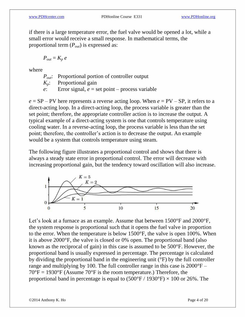
The following figure illustrates a proportional control and shows that there is

always a steady state error in proportional control. The error will decrease with

increasing proportional gain, but the tendency toward oscillation will also increase.

Let’s look at a furnace as an example. Assume that between 1500°F and 2000°F,

the system response is proportional such that it opens the fuel valve in proportion

to the error. When the temperature is below 1500°F, the valve is open 100%. When

it is above 2000°F, the valve is closed or 0% open. The proportional band (also

known as the reciprocal of gain) in this case is assumed to be 500°F. However, the

proportional band is usually expressed in percentage. The percentage is calculated

by dividing the proportional band in the engineering unit (°F) by the full controller

range and multiplying by 100. The full controller range in this case is 2000°F –

70°F = 1930°F (Assume 70°F is the room temperature.) Therefore, the

proportional band in percentage is equal to (500°F / 1930°F) × 100 or 26%. The





engineer can adjust the proportional band and make the system more or less

responsive to an error. The rule of thumb is that a smaller the proportional band (or

large gain) results in a large output or faster response to a given input error, and a

larger band (or small gain) results in a less responsive controller. However, one

must be aware that an excessively large proportional gain will lead to process

instability and oscillation.

One may see that there are issues with proportional control only. One of these

issues is that proportional control cannot compensate for very small errors. (These

errors are also known as offset.) Another issue is that it cannot adjust its output

based on the rate of change in the measured variable. For example, if you are

driving on the highway at 55 miles per hour and the car in front of you slows

down, you may respond by applying 50% brake pressure. This is a proportional

response, because the car in front is slowing down but not coming to a stop.

However, if the car slows down even more, you will apply more brake pressure,

since the car in front’s rate of stopping is greater. In other words, we apply more

brake pressure as we see the distance between our cars getting smaller, because we

naturally respond to the rate of change of error. However, proportional control

systems do not do this; they only respond to the magnitude of the error, not to its

rate of change.

2.2. Integral Control

To address the first issue with the proportional control, integral control attempts to

correct a small error (offset). The integral examines the error over time and

increases the importance of even a small error over time. The integral is equal to

error multiplied by the time the error has persisted. A small error at time zero has

zero importance. A small error at time 10 has an importance of 10 times error. As

such, the integral increases the response of the system to a given error over time

until it is corrected. The integral can also be adjusted, and the adjustment is called

the reset rate. The reset rate is a time factor. The shorter the reset rate, the quicker

the correction of an error. However, too short a reset rate can cause erratic

performance. In hardware-based systems, the adjustment can be done by a

potentiometer that changes the time constant of an RC circuit. Most of today’s

applications use a software-based control, such as a PLC module, through which

the engineer changes the parameter of the reset rate. The mathematical expression

of an integral-only controller (Iout) is:





where

Iout: Integral portion of controller output

Ti: Integral time, or reset time

Ki: Integral gain


2.3. Derivative Control

The derivative part of the control output attempts to look at the rate of change in

the error signal. The derivative will cause a greater system response to a rapid rate

of change than to a small rate of change. In other words, if a system’s error

continues to rise, the controller must not be responding with sufficient correction.

The derivative senses this rate of change in the error and provides a greater

response. The derivative is adjusted as a time factor and therefore is also called rate

time. It is essential that too much derivative should not be applied or it can cause

overshoot or erratic control. In mathematical terms, the derivative term (Dout) is

expressed as:

where

Dout: Derivative portion of controller output

Td: Derivative time

Kd: Derivative gain


To summarize the tasks of all three controls, proportional control causes an input

signal to change as a direct ratio of the error signal variation. It responds

immediately to the current tracking error, but it cannot achieve the desired set point

accuracy without an unacceptably large gain. Thus, the proportional term usually

needs the other terms. Integral control causes the output signal to change as a

function of the integral of the error signal over time duration. The integral term

yields zero steady state error in tracking a constant set point. It also rejects constant

disturbances. Derivative action reduces transient errors and causes an output signal

to change as a function of the rate of change of the error signal. The contributions

of the three terms will yield the control output, or the control variable:





Control Variable = Pout + Iout + Dout

The following figure illustrates a closed-loop system with proportional, integral,

and derivative control. (Closed-loop system will be defined later.)

In practice, most PID controllers can be run in two modes: manual or automatic. In

manual mode, the controller output is manipulated directly by the operator,

typically by pushing buttons that increase or decrease the controller output. A

controller may also operate in combination with other controllers, such as in a

cascade or ratio connection, or with nonlinear elements, such as multipliers and

selectors. In automatic mode, the PID parameters can be adjusted during operation.

When there are changes of modes and parameters, it is important to avoid

switching transients.

Since the PID controller is a dynamic system, it is necessary to make sure the state

of the system is correct when switching the controller between manual and

automatic mode. When the system is in automatic mode, the PID algorithm

produces a control variable that may be different from the manually generated

control variable. Therefore, it is crucial for the operator to make sure the two

control variables match at the time of switching. This is called bumpless transfer.

The first scenario is switching from automatic to manual. A bumpless transfer will

force the manual output to track the output of the controller. If no disturbances

occur after switching, the PV will not change. The second scenario is switching

from manual to automatic. If the PV is not equal to the SP, the switch will result in

an immediate “bump” to the controller output due to proportional action. To avoid

the immediate bump, the operator can do one of the following: 1) adjust the SP to

the current PV and then switch to automatic and slowly change the SP; 2) slowly

adjust the controller output until the PV equals the current SP and then switch to

automatic; or 3) use SP tracking while in manual. This would force the current SP

to track the PV while in manual so that no proportional bump occurs while

switching to automatic.





Below is the pseudo-code of a simple software loop that implements a feedback

PID algorithm.

Constants:

Gain System gain

ResetRate Reset rate

Derivative Derivative

Variables:

Input Process input

InputDev Process input plus derivative

InputPrev Process input from previous pass, used in derivative calculation

Error Difference between input and set point

Setpt Set point

OutputTemp Temporary value of output

Output Output of PID algorithm

Feedback Result of time delay in positive feedback loop (Sometimes this

is called the manual reset or bias)

Mode Value is “AUTO” if loop is in automatic

Action Value is “DIRECT” if loop is direct acting

IF Mode = “AUTO” THEN

InputDev = Input + (Input – InputPrev) * Derivative * 60 // Derivative

InputPrev = Input

Error = Setpt – InputDev // Error based on reverse action

IF Action = “DIRECT” THEN

Error = 0 – Error // Change sign of error for direct action

ENDIF

OutputTemp = Error * Gain + Feedback

// Limit output to 0 – 100%

IF OutPutTemp > 100 THEN OutPutTemp = 100

IF OutPutTemp < 0 THEN OutPutTemp = 0

Output = OutputTemp // The final output of the controller.

Feedback = Feedback + (Output – Feedback) * ResetRate / 60

ELSEIF Mode = “MANUAL” THEN

InputPrev = Input // Stay ready for bumpless switch to Auto

Feedback = Output

ENDIF





Feedback control corrects any cumulative measurement errors or other errors in the

system. In contrast, feedforward control applies to a system in which a balance

between supply and demand is achieved by measuring both demand potential and

demand load and using this information to govern supply. Feedforward control

applies to a process that must be completely understood and requires no special

instrumentation. Feedforward is often used to control processes with transportation

and measurement lags. For example, a feedforward value representing “cold water

poured into a warm mix” could boost the output value faster than waiting for the

process variable to change as a result of the mixing. Another example is that the

lag between input and output in a distillation column may vary from a few minutes

to many minutes, depending on the size of the column and other variables. When

long lags are inherent to this process, feedback control becomes difficult, because

it cannot make any required corrections until the error is sensed. Feedforward can

be used to reduce the lag and improve control results, because an exact balance

between supply and demand potential is achieved before the process is influenced.

3. Implementation of PID Control

As suggested earlier, to implement a PID control, the engineer must first choose

the structure of the PID controller and then must choose numerical values for the

PID coefficients to tune the controller.

3.1. Choosing the Structure of a PID Controller

To choose the structure of a controller, refer to the following table of tuning effects

of the PID controller terms. This is a reference table that shows how each term of

the controller can be selected to accomplish a particular closed-loop system effect

of specification.

Reference Tracking Tuning Disturbance Rejection Tuning

Step Reference Constant Load Disturbance

Transient Steady State Transient Steady State

P Increasing Kp > 0

speeds up the

response.

Increasing Kp > 0

reduces but does

not eliminate

steady state

offset.

Increasing Kp > 0

speeds up the

response.

Increasing Kp > 0

reduces but does

not eliminate

steady state

offset.





I Introducing

integral action Ki

> 0 gives a wide

range of

response types.

Introducing

integral action Ki

> 0 eliminates

offset in the

reference

response.

Introducing

integral action Ki

> 0 gives a wide

range of

response types.

Introducing

integral action Ki

> 0 eliminates

steady state

offsets.

D Derivative action

Kd > 0 gives a

wide range of

responses and

can be used to

tune response

damping.

Derivative action

has no effect on

steady state

offset.

Derivative action

Kd > 0 gives a

wide range of

responses and

can be used to

tune response

damping.

Derivative action

has no effect on

steady state

offset.

Let’s consider this example: if it is necessary to remove steady state offsets from a

closed-loop output response, the table indicates that a D-term will not do this and a

P-term will reduce the offset if the proportional gain Kp is increased, but an I-term

will eliminate the offset completely. Therefore, an integral term would be chosen

for inclusion in the controller structure. Another example occurs when the engineer

has elected to use integral action to eliminate constant steady state process

disturbance offset errors but now wishes to speed up the closed-loop system

response. The table shows that increasing the proportional gain Kp will have just

this effect, so both proportional (P) action and integral (I) action would be selected,

giving a PI controller solution.

The examples above show how the PID controller structure is selected to match the

desired closed-loop performance. This selection process can be simplified using

the following PID term selection flow diagram.





3.2. Tuning the PID Controller

The second part of setting up a PID controller is to tune or choose numerical values

for the PID parameters. PID controllers are tuned in terms of their P, I, and D

terms. Tuning the control gains can result in the following improvements of

responses:

Proportional gain (Kp)

Larger proportional gain typically means faster response, because the larger the

error, the larger the proportional term compensation. However, an excessively

large proportional gain may result in process instability and oscillation.

Integral gain (Ki)

Larger integral gain implies that steady state errors are eliminated faster.

However, the trade-off may be a larger overshoot, because any negative error

integrated during transient response must be integrated away by positive error

before steady state can be reached.

Derivative gain (Kd)

Larger derivative gain decreases overshoot but slows down transient response

and may lead to instability due to signal noise amplification in the

differentiation of the error.

The following table lists some common tuning methods and their advantages and

disadvantages. The choice of method will mostly depend on whether or not the

loop can be taken offline for tuning and the response time of the system. If the

system can be taken offline, the best tuning method often involves subjecting the

system to a step change in input, measuring the output as a function of time, and

using this response to determine the control parameters. Manual tuning methods

can be quite inefficient, especially if the loops have response times of longer than a

minute.

Tuning

Method

Advantages Disadvantages

Manual tuning No math required

Online method

Requires experienced

personnel

Ziegler-

Nichols Proven method

Online method

Process upset

Some trial and error

Very aggressive tuning





Software tools Consistent tuning

Either online or offline tuning

May include actuator and

sensors analysis

Involves some cost and

training

Cohen-Coon Good process models

Requires some math

Offline method only

Only good for first-order

process

Many manufacturing and industrial process companies have in-house guidelines

for tuning PID controllers in particular process plant units. Therefore, it is often

possible to provide rules and empirical formulas for PID controller tuning

procedures. Some of these guidelines base their procedures on the routines of the

commonly used Ziegler-Nichols methods. The two Ziegler-Nichols methods use an

online process experiment followed by a set of rules to calculate the numerical

values of the PID parameters. Numerous improvements and extensions of the

associated rules have been achieved since their introduction.

Ziegler-Nichols is a type of continuous cycling method for controller tuning. The

term continuous cycling refers to a continuous oscillation with constant amplitude

and is based on trial-and-error procedure. The following are the steps to implement

the method:

1. Allow the process to reach steady state as much as possible, turn off the integral

mode (or set time to zero), and then turn off the derivative mode.

2. Assign a small value to proportional-only controller gain K (e.g., 0.5), and place

the controller in automatic mode.

3. Make a small set point change so that the control variable moves away from the

set point.

4. Increase the gain slightly.

5. Repeat steps 3 and 4 until continuous oscillation is achieved. This is known as

the ultimate gain.

6. Calculate the PID controller settings using the Ziegler-Nichols tuning relations

in the following table.





7. Evaluate the Ziegler-Nichols controller settings by introducing a small set point

change and observing the closed-loop response. Fine tune the settings if

necessary.

P Control PI Control PID Control

Kp 0.5 K 0.45 K 0.6 K

Ki

Kd

Note: K is the ultimate gain (the gain at which the oscillations continue with

constant amplitude), and T is the time or ultimate period in minutes measured in

the gain calibration above (the time it takes the process variable to complete one

full oscillation while the system is at steady state).

By tuning the three parameters in the PID controller algorithm, the controller can

provide control action designed for specific process requirements. The controller’s

response can be described in terms of the controller’s responsiveness to error, the

degree to which the controller overshoots the set point, and the degree of system

oscillation. Note that the use of the PID algorithm for control does not guarantee

optimal control of the system or system stability. Some applications may require

using only one or two modes to provide the appropriate system control. A PID

controller will be called a P, I, PI, or PD controller in the absence of respective

control actions. If the PID controller parameters are improperly chosen, the

controlled process input can become unstable. Instability is often caused by excess

gain, particularly in the presence of significant time delay. In most applications,

stability of response is required, and the process must not oscillate for any

combination of process conditions.

4. Open-Loop vs. Closed-Loop Control

An open-loop controller, also called a non-feedback controller, computes its input

into a system using only the current state and its model of the system. The





controller does not receive a feedback signal from the process and it only has a set-

point and a fixed output signal. The output signal does not change, regardless of

the system conditions and disturbances. Consequently, an open-loop system cannot

engage in machine learning or correct any error that it produces. It also may not

compensate for disturbances in the system.

For example, an irrigation sprinkler system programmed to turn on at fixed times is

an example of an open-loop system if it does not measure soil moisture as a form

of feedback. Even when it is raining, the sprinkler system would still activate on

schedule.

An open-loop controller is often used in simple processes because of its simplicity

and low cost, particularly in systems where feedback is not critical. A typical

example would be a conventional dryer, for which the length of machine drying

time is entirely based on the judgment and estimation of the human operator. To

obtain a more accurate or more adaptive control, it is necessary to feed the output

of the system back to the controller. This type of system is called a closed-loop

system.

In a closed-loop system, also called a feedback system, the controller has a

feedback signal from the process. The controller has a set point, a feedback input

signal, and a varying output signal. The output signal increases or decreases

proportionally to the error of the set point compared to the input signal. The input

signal varies proportionally to the system disturbances and the gain of the

measurement sensor.

An example of a closed-loop system would be an automobile’s cruise control.

When the car goes up a hill, the car will power up to maintain the set point speed

set by the driver; the steeper the hill, the more power will be applied. The increase

in slope is a system disturbance, but there can be more than one disturbance on a

system. A stronger head wind would add to the error of an increasing slope,

requiring the car use even more power to keep up with the set point.

5. Example: PID Controller for DC Motor

In this example, the desired target speed of the motor is set by the user. This value

is fed into the speed controller to change the motor speed, and the loop is closed by

a tachometer. The controller constantly adjusts the value of the DC voltage applied

to the motor to maintain the desired speed. The control loop is shown in the

following figure:





The speed controller contains two components: speed control and a digital-to-

analog converter. The speed control component compares the desired speed with

the measured speed and generates a digital value proportional to the DC value to

be applied to the motor. The digital-to-analog converter is implemented using a

signal generator and a low pass filter to smooth out the signal.

The transfer function for the DC motor’s speed is expressed in Laplace form as:

where

K: Electromotive force control = 0.01 Nm/Amp

R: Electrical resistance = 1 Ω

L: Electrical inductance = 0.5H

J: Moment of inertia of rotor = 0.01 kg m2/s

2

b: Damping ratio of mechanical system = 0.1 Nms

V: Source voltage

θ: Rotating speed

Therefore, the rotating speed of the motor is directly proportional to the input

voltage. First, let’s try a proportional-only control with a gain (Kp) of 100 and step

input of 1 rad/sec. A step response is received as follows:





From the figure above, we see that both the steady state error and overshoot are too

large. Since adding an integral term will eliminate the steady state error and a

derivative term will reduce the overshoot, we try a PID controller with small Ki = 1

and Kd = 1. After that, the step response curve looks like this:

However, now the settling time is too long. So we increase Ki to 200 to reduce the

settling time. After that, the step response curve looks like the following:





Now we see that the response is much faster than before; however, the large Ki has

worsened the transient response (big overshoot). So we increase Kd to 10 to reduce

the overshoot. After that, the step response curve looks like:

We can now use a PID controller with the following parameters to adjust the value

of the DC voltage applied to the motor to maintain the desired speed.

Kp = 100

Ki = 200

Kd = 10

6. Cascade Control

PID control can be improved by changing the PID parameters, improving

measurement, such as sampling rate, precision, and accuracy, and using low-pass

filtering. Another proven method is cascading multiple PID controllers, which can





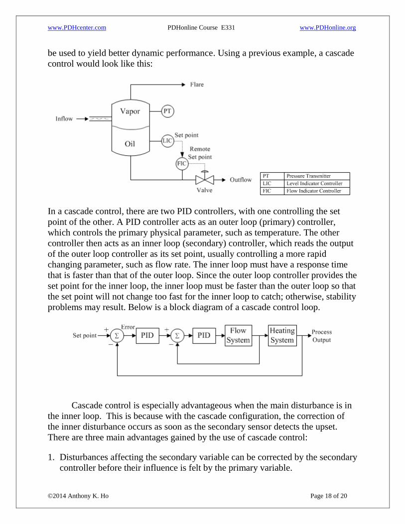
be used to yield better dynamic performance. Using a previous example, a cascade

control would look like this:

In a cascade control, there are two PID controllers, with one controlling the set

point of the other. A PID controller acts as an outer loop (primary) controller,

which controls the primary physical parameter, such as temperature. The other

controller then acts as an inner loop (secondary) controller, which reads the output

of the outer loop controller as its set point, usually controlling a more rapid

changing parameter, such as flow rate. The inner loop must have a response time

that is faster than that of the outer loop. Since the outer loop controller provides the

set point for the inner loop, the inner loop must be faster than the outer loop so that

the set point will not change too fast for the inner loop to catch; otherwise, stability

problems may result. Below is a block diagram of a cascade control loop.

Cascade control is especially advantageous when the main disturbance is in

the inner loop. This is because with the cascade configuration, the correction of

the inner disturbance occurs as soon as the secondary sensor detects the upset.

There are three main advantages gained by the use of cascade control:

1. Disturbances affecting the secondary variable can be corrected by the secondary

controller before their influence is felt by the primary variable.





2. Closing the control loop around the secondary part of the process reduces the

phase lag seen by the primary controller, resulting in increased speed of the

response. Because of the increased speed of response, the sensitivity of the

primary process variable to process upsets is also reduced.

3. The use of the secondary loop can reduce the effect of control valve sticking or

actuator nonlinearity.

7. Troubleshooting PID Control

If a control loop is not performing satisfactorily, troubleshooting is necessary to

identify the source of the problem. In many process applications, a control loop

that once operated satisfactorily can become either unstable or excessively sluggish

for a variety of reasons, including:

Changing process conditions, usually changes in throughput rate

A sticking control valve stem

A plugged line in a pressure or differential pressure transmitter

Fouled heat exchangers, particularly reboilers for distillation columns

Cavitating pumps (usually caused by a suction pressure that is too low)

The starting point for troubleshooting is to obtain enough background information

to define the problem clearly. The following questions must be answered:

What are the control objectives?

What is the process being controlled?

What are the control variables?

Are closed-loop response data available?

Is the controller in manual or automatic mode? Is it reverse or direct acting?

If the process is cycling, what is the cycling frequency?





What PID controller algorithm is used? What are the PID controller

parameters?

Is the process open-loop stable?

What additional documentation is available, such as control loop summary

sheets, piping and instrumentation diagrams (P&ID), etc.?



fundamental of pid control - pdhonline.com · fundamental of pid control anthony k. ho ... fairfax,...

Documents