fully probabilistic seismic source inversion – part 1 ... · fully probabilistic seismic source...

Solid Earth, 5, 1055–1069, 2014www.solid-earth.net/5/1055/2014/doi:10.5194/se-5-1055-2014© Author(s) 2014. CC Attribution 3.0 License.

Fully probabilistic seismic source inversion – Part 1: Efficientparameterisation

S. C. Stähler1 and K. Sigloch1,2

1Dept. of Earth and Environmental Sciences, Ludwig-Maximilians-Universität (LMU), Munich, Germany2Dept. of Earth Sciences, University of Oxford, South Parks Road, Oxford OX1 3AN, UK

Correspondence to:S. C. Stähler ([email protected])

Received: 3 July 2013 – Published in Solid Earth Discuss.: 23 July 2013Revised: 14 October 2013 – Accepted: 28 October 2013 – Published: 17 November 2014

Abstract. Seismic source inversion is a non-linear prob-lem in seismology where not just the earthquake param-eters themselves but also estimates of their uncertaintiesare of great practical importance. Probabilistic source in-version (Bayesian inference) is very adapted to this chal-lenge, provided that the parameter space can be chosen smallenough to make Bayesian sampling computationally feasi-ble. We propose a framework for PRobabilistic Inferenceof Seismic source Mechanisms (PRISM) that parameterisesand samples earthquake depth, moment tensor, and sourcetime function efficiently by using information from previ-ous non-Bayesian inversions. The source time function isexpressed as a weighted sum of a small number of empir-ical orthogonal functions, which were derived from a cata-logue of> 1000 source time functions (STFs) by a princi-pal component analysis. We use a likelihood model based onthe cross-correlation misfit between observed and predictedwaveforms. The resulting ensemble of solutions provides fulluncertainty and covariance information for the source pa-rameters, and permits propagating these source uncertaintiesinto travel time estimates used for seismic tomography. Thecomputational effort is such that routine, global estimationof earthquake mechanisms and source time functions fromteleseismic broadband waveforms is feasible.

1 Introduction

Seismic source inversion is one of the primary tasks of seis-mology, and the need to explain devastating ground move-ments was at the origin of the discipline. The interest is tolocate the earthquake source using seismogram recordings,

and to combine this information with geological knowledge,in order to estimate the probability of further earthquakesin the same region. This purpose is served well by a vari-ety of existing source catalogues, global and regional. Largeearthquakes and those in densely instrumented areas are be-ing studied in detail, using extended-source frameworks likefinite-fault or back-projection.

Smaller earthquakes (MS ≤ 7.5), and especially remoteevents with sparse data coverage, are better parameterisedby a point source. Most catalogues determine only a loca-tion and a moment tensor solution, which often allows foridentification of the associated fault. But the waveform datacontain additional information: for earthquakes exceedingMS ≥ 5.5, it is generally possible to invert for the tempo-ral evolution of the rupture, described by a time series calledthe source time function (STF) (Ruff, 1989; Houston, 2001).While the STF may further aid the understanding of earth-quake mechanisms (Vallée, 2013) and hazard or the interpre-tation of an event in a mining context (Gibowicz, 2009), ourprimary motivation for estimating it is a different one: theSTF convolves the broadband Green function and stronglyaffects its waveform. Waveform tomography estimates three-dimensional earth structure by optimising the fit of observedto predicted waveforms, but at high frequencies (e.g. ex-ceeding 0.1 Hz) such fits can only succeed when the sourcetime function is incorporated into the predicted waveform(Sigloch and Nolet, 2006; Stähler et al., 2012). Hence thepurpose here is to develop an automated procedure to rou-tinely estimate broadband source time functions and pointsource parameters from global seismogram recordings, in-cluding a full treatment of parameter uncertainties.

Published by Copernicus Publications on behalf of the European Geosciences Union.

1056 S. C. Stähler and K. Sigloch: Bayesian source inversion Part 1

A few recent catalogues now include STF estimates(Vallée et al., 2011; Garcia et al., 2013), but the treatmentof parameter uncertainties is still incomplete. Uncertain-ties in the STF correlate most strongly with source depthestimates, especially for shallow earthquakes (Sigloch andNolet, 2006), where surface-reflected phases (pP, sP) in-evitably enter the time window for STF estimation (seeFig.1). Inversion for the STF and the moment tensor is linear,whereas inversion for depth is inherently non-linear. Hencegradient-free optimisation techniques like simulated anneal-ing (Kirkpatrick et al., 1983) or the first stage of the neigh-bourhood algorithm (NA) (Sambridge, 1999a) have becomepopular; Table4 presents an overview of gradient-free sourceinversion algorithms from recent years. These optimisationalgorithms provide only rudimentary uncertainty estimates.

A natural alternative, pursued here, is Bayesian sampling,where an ensemble of models is generated. The membersof this ensemble are distributed according to the posteriorprobability densityP(m), wherem is the model parametervector to estimate. Integrating over certain parameters of thisjoint posteriorP(m), or linear combinations thereof, yieldsmarginal distributions over arbitrary individual parameters orparameter combinations. To the best of our knowledge, en-semble sampling in the context of source parameter estima-tion has been tried twice so far (Wéber, 2006; Debski, 2008),and has been limited to a few events in either case.

A hurdle to using sampling algorithms has been the ef-ficient parameterisation of the source time function. Wepropose a parameterisation based on empirical orthogonalwavelets (Sect.2.1), which reduces the number of free pa-rameters to less than 12 for the STF, and to around 18 in to-tal. We show that this makes Bayesian sampling of the entiremodel space computationally feasible.

A normalised moment tensor is sampled explicitly, andthe scalar moment and absolute values forMj are derivedfrom the amplitude misfit (Sect.2.2). Section3 introducesBayesian inference as a concept and explains the modelspace and prior assumptions. The ensemble inference is donewith the neighbourhood algorithm (Sambridge, 1999a, b). InSect.4, the code is applied to a magnitude 5.7 earthquake inVirginia, 2011. Section5 discusses aspects of our algorithmand potential alternatives, which we compare to related stud-ies by other workers in Sect.5.4and in the Appendix.

Our procedure is called PRISM (PRobabilistic Inferenceof Source Mechanisms); by applying it routinely, we plan topublish ensemble solutions for intermediate-size earthquakesin the near future. A usage of uncertainty information gainedfrom the ensemble is demonstrated in Sect.4.3, where theinfluence of source uncertainties on tomographic travel timeobservables is estimated. Further investigations of noise andof inter-station covariances are presented in a companion pa-per (Stähler et al., 2014).

Fig. 1. Source time function solutions for a MW 5.7 earthquake in Virginia, USA (2011/08/23) obtained from

joint inversion for STF and moment tensor M , using the iterative linearised optimisation algorithm of Sigloch

and Nolet (2006). Trial source depths ranged from 2 km to 17 km, in increments of 1 km, and each decon-

volution was based on the same 86 broadband, teleseismic P-waveforms. Note the strong changes in STF and

moment tensor as a function of depth. Top left shows the moment tensor solution from the NEIC catalogue for

comparison. For every candidate solution, the percentage of “non-negative” energy is given, a proxy for how os-

cillatory (and thus inherently non-physical) the solution is. The third number gives the average cross-correlation

coefficient between observed and predicted waveforms achieved by each solution. At depths between 2 and 7

km, the STF is pulse-like, simple, non-negative, and waveform cross-correlation attains its maximum, signalling

the most likely depth range for this event. The present study offers an approach to quantify these qualitative

tradeoffs and judgements.

4

Figure 1.Source time function solutions for aMW5.7 earthquake inVirginia, USA, (2011/08/23) obtained from joint inversion for STFand moment tensorM, using the iterative linearised optimisationalgorithm ofSigloch and Nolet(2006). Trial source depths rangedfrom 2 km to 17 km, in increments of 1 km, and each deconvolutionwas based on the same 86 broadband, teleseismicP waveforms.Note the strong changes in STF and moment tensor as a functionof depth. Top left shows the moment tensor solution from the NEICcatalogue for comparison. For every candidate solution, the percent-age of “non-negative” energy is given, a proxy for how oscillatory(and thus inherently non-physical) the solution is. The third num-ber gives the average cross-correlation coefficient between observedand predicted waveforms achieved by each solution. At depths be-tween 2 and 7 km, the STF is pulse-like, simple, and non-negative,and waveform cross-correlation attains its maximum, signalling themost likely depth range for this event. The present study offers anapproach to quantify these qualitative tradeoffs and judgements.

Solid Earth, 5, 1055–1069, 2014 www.solid-earth.net/5/1055/2014/

S. C. Stähler and K. Sigloch: Bayesian source inversion Part 1 1057

2 Method

2.1 Parameterisation of the source time function

Source time function (STF) is a synonym for the momentrate m(t) of a point source, denoting a time series that de-scribes the rupture evolution of the earthquake. It is relatedto u(t), the vertical or transverse component of the displace-ment seismogram observed at locationr r by convolutionwith the Green function:

u(t) =

3∑j=1

3∑k=1

∂Gj

∂xk

(rs,r r, t) ∗ s(t) · Mj,k, (1)

wheres(t) ≡ m(t) is the STF;Mj,k denotes the elements ofthe symmetric, 3× 3 moment tensor,M; andG(rs, r r, t) isthe Green function between the hypocentrers and receiverlocationr r.

Due to the symmetry ofM, we can reduce Eq. (1) to asimpler form:

u(t) =

6∑j=1

gl(t) · s(t) · Ml, (2)

whereMl are the unique moment tensor elements andgl

are the respective derivatives of the Green function. The el-ementsgj are not 3-D vectors because we compute eitheronly its vertical component (forP waves) or its transversecomponent (for SH waves). In either case,g is a superpo-sition of six partial functionsgj , corresponding to contribu-tions from six unique moment tensor elementsMl , with aweighting for the non-diagonal elements ofM, which appeartwice in Eq. (1). The orientation of the source is consideredto remain fixed during the rupture – i.e.,Ml does not dependon t – so that a single time seriess(t) is sufficient to describerupture evolution.

For intermediate-size earthquakes (5.5 < MW < 7.0) theSTF typically has a duration of several seconds, which isnot short compared to the rapid sequence of P–pP–sP orS–sS pulses that shallow earthquakes produce in broadbandseismograms. Most earthquakes are shallow in this sense,i.e., shallower than 50 km. In order to assemble tomography-sized data sets, it is therefore imperative to account for thesource time function in any waveform fitting attempt thatgoes to frequencies above≈ 0.05 Hz (Sigloch and Nolet,2006).

Equations (1) and (2) are linear ins(t), so thats(t) can bedetermined by deconvolvingg from u if Mj in consideredfixed. However,g depends strongly on source depth (thirdcomponent of vectorrs), so that a misestimated source depthwill strongly distort the shape of the STF, as demonstratedby Fig.1. Another complication is present in the fact that ob-served seismogramsu(t) (as opposed to the predicted Greenfunctions) are time-shifted relative to each other due to 3-Dheterogeneity in the earth, and should be empirically alignedbefore deconvolvings(t).

These issues can be overcome by solving iteratively fors(t) and Mj with a fixed depth (Sigloch and Nolet, 2006;Stähler et al., 2012), but the approach requires significant hu-man interaction, which poses a challenge for the amounts ofdata now available for regional or global tomography. More-over, such an optimisation approach does not provide sys-tematic estimates of parameter uncertainties.

Monte Carlo sampling avoids the unstable deconvolutionand permits straightforward estimation of full parameter un-certainties and covariances. However, the model space tosample grows exponentially with the number of parameters,and the STF adds a significant number of parameters. Ina naive approach, this number could easily be on the order of100, i.e., computationally prohibitive. For example, the STFsdeconvolved in Fig.1 were parameterised as a time series of25 s duration, sampled at 10 Hz, and thus yielding 250 un-knowns – not efficient, since neighbouring samples are ex-pected to be strongly correlated. This raises the question ofhow many independent parameters or degrees of freedom thisproblem actually has.

Due to intrinsic attenuation of the earth, the high-est frequencies still significantly represented in teleseismicP waves are around 1 Hz. If from experience we requirea duration of 25 s to render the longest possible STFs oc-curring for our magnitude range (Houston, 2001), then thetime-bandwidth product is 1Hz· 25s= 25, and the problemcannot have more degrees of freedom than that.

Efficient parameterisation then amounts to finding a basisof not more than 25 orthogonal functions that span the sub-space of the real-world, band-limited STFs just described. Infact, we can empirically decrease the number of parameterseven further. By the method ofSigloch and Nolet(2006), wehave semi-automatically deconvolved more than 3000 broad-band STFs while building data sets for finite-frequency to-mography. Of these, we propose to use the 1000 STFs thatwe consider most confidently determined as prior informa-tion for what the range of possible STFs looks like, for earth-quakes of magnitude 5.5 < MW < 7.5. By performing a prin-cipal component analysis on this large set of prior STFs, wefind that only around 10 empirical orthogonal wavelets areneeded to satisfactorily explain almost all of the STFs, asshown in Fig.2.

In concrete terms, we applied the MATLAB functionprin-comp.mto a matrix containing the 1000 prior STFs in itsrows. The mean over the matrix columns (time samples)was subtracted prior to performing the decomposition, andis shown in Fig.2a as wavelets0(t). Principal componentanalysis then determiness1(t) as the function orthonormalto s0(t) that explains as much of the variance in the ma-trix rows as possible. After subtracting (optimally weighted)s1(t) from each row, functions2(t) is determined such thatit is orthonormal tos0(t) ands1(t), and explains as much aspossible of the remaining variance. Each subsequent iterationgenerates another orthonormalsi until i = 256, the numberof time samples (matrix columns). The source time function

www.solid-earth.net/5/1055/2014/ Solid Earth, 5, 1055–1069, 2014


Figure 2. Efficient parameterisation of the STF in terms of empiri-cal orthogonal functions, computed from a large set of manually de-convolved STFs that effectively serve as prior information.(a) First16 members of the basis of empirical orthogonal functions.(b) Me-dian RMS misfit between members of the prior STF catalogue andtheir projection on a subspace of the model space spanned by thefirst wavelet basis functions.(c) A typical STF from the catalogue,and its projection onto several subspaces spanned by the first fewbasis functions (N = [4,8,12]).

can now be expressed as

s(t) =

256∑i=1

aisi(t) + s0(t). (3)

In this parameterisation, the new unknowns to solve for dur-ing source estimation are theai . Since principal componentanalysis has sorted theai by their importance to explaininga typical STF, we may choose to truncate this sum at a rela-tively low valueN � 256:

sN (t) =

N∑i=1

aisi(t) + s0(t). (4)

In practice,N will be chosen based on the residual misfitbetweens(t) and sN (t) that one is willing to tolerate. Fig-ure2b shows the dependence of this misfit onN . If we tol-erate an average root mean square (RMS) misfit of 10 % intotal signal variance,N = 10 base functions are sufficient,compared to 16, when using asincbase. In the following weuseN = 12.

A set of potentially problematic STFs expressed by ourbase functions is shown in an electronic supplement to thispaper.

2.2 Parameterisation of the moment tensor

The orientation of the source can be parameterised eitherby a moment tensor using 6 parameters or as a pure shear

displacement source (Aki and Richards, 2002, p. 112) withstrike, slip and dip (to which a term for an isotropic com-ponent might be added). Here we want to estimate the non-double-couple content of the solutions, and hence we sam-ple the full moment tensor. The scalar moment is fixed to 1,so that only relativeMj are estimated. This is equivalent tosampling a hypersphere in the six-dimensional vector space{Mxx,Myy,Mzz,Mxy, Myz,Mxz} with

M0 =1

√2

√M2

xx + M2yy + M2

zz + 2(M2xy + M2

yz + M2xz)

= 1. (5)

Uniform sampling on an-D hypersphere can be achievedby the method ofTashiro (1977), which transformsn − 1uniformly distributed random variablesxi to producen ran-dom variablesri that are distributed uniformly on a hyper-

sphere with√∑6

i=1 r2i = 1. We identifyri with the moment

tensor components and note that the non-diagonal elementsMkl,k 6= l appear twice in the sum (thus we actually samplean ellipsoid rather than a hypersphere). We then have

xi ∼ U(0,1), i = 1,2, . . . ,5

Y3 = 1; Y2 =√

x2; Y1 = Y2x1

Mxx/M0 =

√Y1 · cos(2πx3)

√2

Myy/M0 =

√Y1 · sin(2πx3)

√2 (6)

Mzz/M0 =

√Y2 − Y1 · cos(2πx4)

√2

Mxy/M0 =

√Y2 − Y1 · sin(2πx4)

Myz/M0 =

√Y3 − Y2 · cos(2πx5)

Mzx/M0 =

√Y3 − Y2 · sin(2πx5)

2.3 Forward simulation

Broadband, teleseismic Green’s functions for P–pP–sP andSH–sSH wave trains are calculated by the WKBJ codeof Chapman(1978), using IASP91 (Kennett and Engdahl,1991) as the spherically symmetric reference model for themantle. The reference crust at the receiver site is replacedby a two-layered crust predicted by the model CRUST2.0(Bassin et al., 2000). It uses the mean of layers 3–5 (softsediments, hard sediments, upper crust) from the surface tothe Conrad discontinuity and the mean of layers 6 and 7(middle crust and lower crust) between the Conrad and theMoho. Values for intrinsic attenuation in mantle and crustare taken from the spherically symmetric earth model PREM(Dziewonski, 1981). The synthetic waveforms are comparedto the observed seismograms in time windows that start 10 sbefore the theoreticalP wave arrival time (according toIASP91) and end 41.2 s after.



3 Source parameter estimation by Bayesian sampling

3.1 Bayesian inversion

Bayesian inversion is an application of Bayes’ rule:

P(m|d) =P(d|m)P (m)

P (d), (7)

wherem is a vector of model parameters (in our case depth,moment tensor elementsMj and STF weightsai), andd isa vector of data, i.e., a concatenation ofP and SH wave-forms. These quantities are considered to be random vari-ables that follow Bayes’ rule. We can then identifyP(m)

with the prior probability density of a model. This is the in-formation on the model parameters that we have independentof the experiment. The conditional probability ofd givenm,P(d|m), also calledL(m|d), is thelikelihoodof a modelmto produce the datad. TermP(d) is constant for all modelsand is therefore dropped in what follows.P(m|d) is calledthe posterior probability density (short, “the posterior”) anddenotes the probability assigned to a modelm after havingdone the experiment.

P(m|d) = P(m)L(m|d)k−1 (8)

Since the posteriorP(m|d) may vary by orders of magnitudefor differentd, we work with its logarithm. We introduce thequantity8(m|d) to denote some kind of data misfit such thatthe likelihood can be written asL(m) = exp[−8(m|d)].

ln(P (m|d)) = −8(m|d) + lnP(m) − lnk (9)

The normalisation constantk is

k =

∫exp[−8(m|d)]P(m)dm (10)

and calculated by the neighbourhood algorithm in the ensem-ble inference stage.

In the case of multivariate, Gaussian-distributed noise onthe data with a covariance matrixSD,

d = g(m) + ε, ε ∼N (0,SD), (11)

whereg(m) is the data predicted by modelm, we would ob-tain the familiar expression

8(m|d) = k′

(1

2(d − g(m))T S−1

D (d − g(m))

). (12)

This term is usually called Mahalanobis distance or`2-misfit.We do not choose this sample-wise difference between ob-

served and predicted waveforms as our measure of misfit.There are questions about the Gaussian noise assumption forreal data, but mainly we consider there to be a measure that ismore robust and adapted to our purpose, the cross-correlation(mis-)fit between data and synthetics (Stähler et al., 2014),

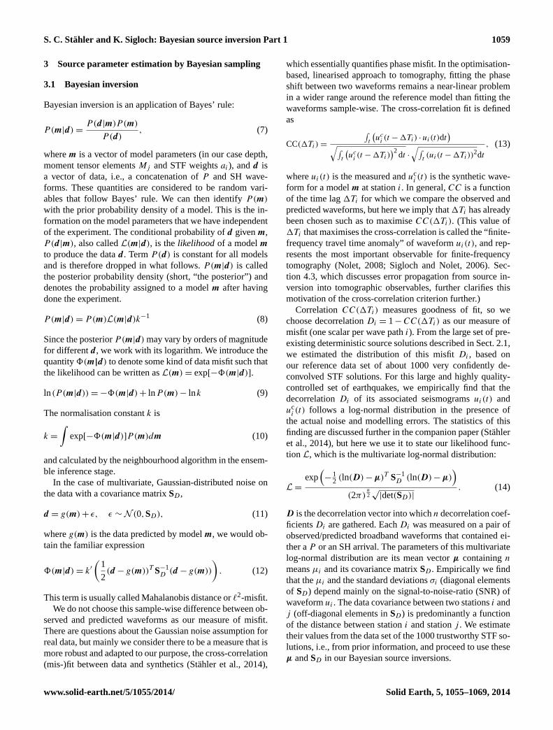
which essentially quantifies phase misfit. In the optimisation-based, linearised approach to tomography, fitting the phaseshift between two waveforms remains a near-linear problemin a wider range around the reference model than fitting thewaveforms sample-wise. The cross-correlation fit is definedas

CC(1Ti) =

∫t

(uc

i (t − 1Ti) · ui(t)dt)√∫

t

(uc

i (t − 1Ti))2dt ·

√∫t (ui(t − 1Ti))

2dt

, (13)

whereui(t) is the measured anduci (t) is the synthetic wave-

form for a modelm at stationi. In general,CC is a functionof the time lag1Ti for which we compare the observed andpredicted waveforms, but here we imply that1Ti has alreadybeen chosen such as to maximiseCC(1Ti). (This value of1Ti that maximises the cross-correlation is called the “finite-frequency travel time anomaly” of waveformui(t), and rep-resents the most important observable for finite-frequencytomography (Nolet, 2008; Sigloch and Nolet, 2006). Sec-tion 4.3, which discusses error propagation from source in-version into tomographic observables, further clarifies thismotivation of the cross-correlation criterion further.)

CorrelationCC(1Ti) measures goodness of fit, so wechoose decorrelationDi = 1− CC(1Ti) as our measure ofmisfit (one scalar per wave pathi). From the large set of pre-existing deterministic source solutions described in Sect.2.1,we estimated the distribution of this misfitDi , based onour reference data set of about 1000 very confidently de-convolved STF solutions. For this large and highly quality-controlled set of earthquakes, we empirically find that thedecorrelationDi of its associated seismogramsui(t) anduc

i (t) follows a log-normal distribution in the presence ofthe actual noise and modelling errors. The statistics of thisfinding are discussed further in the companion paper (Stähleret al., 2014), but here we use it to state our likelihood func-tionL, which is the multivariate log-normal distribution:

L=

exp(−

12 (ln(D) − µ)T S−1

D (ln(D) − µ))

(2π)n2√

|det(SD)|. (14)

D is the decorrelation vector into whichn decorrelation coef-ficientsDi are gathered. EachDi was measured on a pair ofobserved/predicted broadband waveforms that contained ei-ther aP or an SH arrival. The parameters of this multivariatelog-normal distribution are its mean vectorµ containingn

meansµi and its covariance matrixSD. Empirically we findthat theµi and the standard deviationsσi (diagonal elementsof SD) depend mainly on the signal-to-noise-ratio (SNR) ofwaveformui . The data covariance between two stationsi andj (off-diagonal elements inSD) is predominantly a functionof the distance between stationi and stationj . We estimatetheir values from the data set of the 1000 trustworthy STF so-lutions, i.e., from prior information, and proceed to use theseµ andSD in our Bayesian source inversions.



It follows from Eq. (14) that the misfit8 is

8 =1

2

(n∑i

n∑j

(ln(Dj ) − µj

)TS−1

D,ij

(ln(Dj ) − µj

))

+1

2ln((2π)n|det(SD)|

)(15)

3.2 Construction of the prior probability density

A crucial step in Bayesian inference is the selection of priorprobabilitiesP(m) on the model parametersm. Our modelparameters are as follows:

– m1: source depth. We assume a uniform prior basedon the assumed depth of the event in the NationalEarthquake Information Center (NEIC) catalogue. Ifthe event is shallow according to the InternationalSeismological Centre (ISC) catalogue (< 30km), wedraw from depths between 0km and 50km; i.e.,m1 ∼

U(0,50). For deeper events, we draw from depths be-tween 20km and 100km. Events deeper than 100kmhave to be treated separately, using a longer time win-dow in Eq. (13) that includes the surface reflectedphasespPandsP.

– m2, . . . ,m13 = a1, . . . ,a12: the weights of the sourcetime function (Eq.4). The samples are chosen from uni-form distributions with ranges shown in Table1, but aresubjected to a prior,πSTF (see below).

– m14, . . . ,m18 = x1, . . .x5: the constructor variables forthe moment tensor (Eq.6). xi ∼ U(0,1), but they aresubjected to two priors,πiso andπCLVD (see below).

Intermediate-sized and large earthquakes are caused bythe release of stress that has built up along a fault, drivenby shear motion in the underlying, viscously flowing mantle.Hence the rupture is expected to proceed in only one direc-tion, the direction that releases the stress. The source timefunction is defined as the time derivative of the moment,s(t) = m(t). The moment is proportional to the stress andthus monotonous, and hences(t) should be non-negative.In practice, an estimated STF is often not completely non-negative (unless this characteristic was strictly enforced).The reason for smaller amounts of “negative energy” (timesamples with negative values) in the STF include reverber-ations at heterogeneities close to the source, which producesystematic oscillations that are present in most or all of theobserved seismograms. Motivated by waveform tomography,our primary aim is to fit predicted to observed waveforms. Ifa moderately non-negative STF produces better-fitting syn-thetics, then our pragmatic approach is to accept it, sincewe are not interested in source physics per se. However, westill need to moderately penalise non-negative samples in theSTF, because otherwise they creep in unduly when the prob-lem is underconstrained, due to poor azimuthal receiver cov-erage. In such cases, severely negative STFs often produce

Table 1.Sampling of the prior probability distribution: range of STFweightsai that are permitted in the first stage of the neighbourhoodalgorithm.

i Range i Range i Range

1 ±1.5 7 ±0.8 12 ±0.52 ±1.0 8 ±0.7 13 ±0.53 ±0.9 9 ±0.7 14 ±0.44 ±0.8 10 ±0.6 15 ±0.4

marginally better fits by fitting the noise. Smaller earthquakesin other contexts, like mining tremors or dyke collapse involcanic settings, may have strong volume changes involvedand therefore polarity changes in the STF (e.g.Chouet et al.,2003). However, such events are outside of the scope of thisstudy.

Our approach is to punish slightly non-negative STF esti-mates only slightly, but to severely increase the penalty oncethe fraction of “negative energy”I exceeds a certain thresh-old I0. To quantify this, we defineI as the squared negativepart of the STF divided by the entire STF squared:

I =

∫ T

0 sN (t)2· 2(−sN (t))dt∫ T

0 sN (t)2, where (16)

sN = s0(t) +

N∑i=1

aisi(t) (17)

and 2 is the Heaviside function. Based onI , we definea priorπSTF:

πSTF(m2, . . . ,m13) = exp

[−

(I

I0

)3]

, (18)

where the third power andI0 = 0.1 have been found to workbest. In other words, up to 10 % of STF variance may becontributed by negative samples (mostly oscillations) with-out penalty, but any larger contribution is strongly penalizedby the priorπSTF.

The neighbourhood algorithm supports only uniform dis-tributions on parameters. The introduction ofπSTF definedby Eq. (18) leads to a certain inefficiency, in that parts of themodel space are sampled that are essentially ruled out by theprior. We carefully selected the ranges of theai by examin-ing their distributions for the 1000 catalogue solutions. A testwas to count which fraction of random models were consis-tent withI < 0.1. For the ranges given in Table1, we foundthat roughly 10 % of the random STF estimates hadI < 0.1.

A second prior constraint is that earthquakes caused bystress release on a fault should involve no volume change,meaning that the isotropic componentMiso = Mxx + Myy +

Mzz of the moment tensor should vanish. Hence we introduceanother prior constraint,



πiso(m14, . . . ,m18) = exp

[−

(Miso/M0

σiso

)3]

, (19)

whereM0 is the scalar moment, andσiso = 0.1 is chosen em-pirically.

Third, we also want to encourage the source to be double-couple-like. A suitable prior is defined on the compensatedlinear vector dipole (CLVD) content, which is the ratioε =

|λ3|/|λ1| between smallest and largest deviatoric eigenvaluesof the moment tensor:

πCLVD(m14, . . . ,m18) = exp

[−

(ε

σCLVD

)3]

. (20)

In the absence of volume change, a moment tensor withε = 0.5 corresponds to a purely CLVD source, whileε = 0is a pure DC source. Again we have to decide on a sensi-ble value for the characteristic constantσCLVD . We chooseσCLVD = 0.2, which seems to be a reasonable value for theintermediate-sized earthquakes of the kind we are interestedin (Kuge and Lay, 1994).

The total prior probability density is then

P(m) = πSTF(m2, . . . ,m13) (21)

+ πiso(m14, . . . ,m18) + πCLVD(m14, . . . ,m18).

3.3 Sampling with the neighbourhood algorithm

Our efficient wavelet parameterisation of the STF reducesthe total number of model parameters to around 18, but sam-pling this space remains non-trivial. The popular Metropolis–Hastings algorithm (MH) (Hastings, 1970) can handle prob-lems of this dimensionality, but is non-trivial to use for sam-pling multimodal distributions (see the discussion for de-tails). These problems are less severe for a Gibbs sampler,but this algorithm needs to know the conditional distribu-tion p(xj |x1, . . .xj−1,xj+1,xn) along parameterxj in then-dimensional model space (Geman and Geman, 1984). Thisconditional distribution is usually not available, especiallynot for non-linear inverse problems.

To overcome the problem of navigation in complex high-dimensional model spaces, the neighbourhood algorithmuses Voronoi cells (Sambridge, 1998) to approximate a mapof the misfit landscape (Sambridge, 1999a, first stage), fol-lowed by a Gibbs sampler to appraise an ensemble based onthis map (Sambridge, 1999b, second stage).

In order to point the map-making first stage of the NAinto the direction of a priori allowed models, we use a pre-calculated set of starting models. For that, the NA is run with-out forward simulations and without calculating the likeli-hood, so that only a map of the prior landscape is produced,from 32 768 samples (Fig.3a). This means that from the startthe map will be more detailed in a priori favourable regions,and avoids the algorithm wasting too much time refining themap in regions that are essentially ruled out by the prior.

−1 −0.5 0 0.5 1

−1

−0.5

0

0.5

1

Parameter 1

Para

mete

r 2

−1 −0.5 0 0.5 1

−1

−0.5

0

0.5

1

Parameter 1

Para

mete

r 2

−1 −0.5 0 0.5 1

−1

−0.5

0

0.5

1

Parameter 1

Para

mete

r 2

Fig. 3. Principle of the Neighbourhood Algorithm, demonstrated for a two-dimensional toy problem (the un-

derlying distributions are fictional and chosen for demonstration purposes). Top: In the pre-mapping stage,

only the prior distribution is evaluated, resulting in a map of starting models that cluster in regions of high prior

probability (marked by lighter shades of red). Middle: Next, the NA loads this map, evaluates the posterior

probability for every sample, and refines the map only in the best fitting Voronoi cells. Lighter shades of blue

correspond to a higher posterior probability. Bottom: In the sampling or appraisal stage, the value of the poste-

rior is interpolated to the whole Voronoi cell. The Gibbs sampler uses this map to produce an ensemble. This

ensemble can be used to calculate integrals over the model space, like the mean or mode of selected parameters.10

Figure 3. Principle of the neighbourhood algorithm, demonstratedfor a two-dimensional toy problem (the underlying distributions arefictional and chosen for demonstration purposes). Top: in the pre-mapping stage, only the prior distribution is evaluated, resulting ina map of starting models that cluster in regions of high prior proba-bility (marked by lighter shades of red). Middle: next, the NA loadsthis map, evaluates the posterior probability for every sample, andrefines the map only in the best-fitting Voronoi cells. Lighter shadesof blue correspond to a higher posterior probability. Bottom: in thesampling or appraisal stage, the value of the posterior is interpolatedto the whole Voronoi cell. The Gibbs sampler uses this map to pro-duce an ensemble. This ensemble can be used to calculate integralsover the model space, like the mean or mode of selected parameters.



Next, the prior landscape is loaded and a forward simula-tion is run for each member in order to evaluate its posteriorprobability. Then this map is further refined by 512 forwardsimulations around the 128 best models. This is repeated un-til a total of 65 536 models have been evaluated.

In the second stage of the NA, which is the sampling stage,400 000 ensemble members are drawn according to the pos-terior landscape from the first step. This process runs ona 16-core Xeon machine and takes around 2 h in total perearthquake.

4 A fully worked example

4.1 2011/08/23 Virginia earthquake

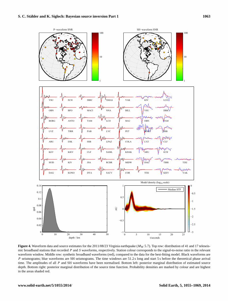
In the following we present a fully worked example fora Bayesian source inversion, by applying our software to theMW 5.7 earthquake that occurred in central Virginia on 23August 2011 (Figs.4 and5, also compare to Fig.1). Whilenot considered a typical earthquake region, events from thisarea have nevertheless been recorded since the early daysof quantitative seismology (Taber, 1913). Due to its occur-rence in an unusual but densely populated area, this relativelysmall earthquake was studied in considerable detail, afford-ing us the opportunity to compare to results of other workers.Moderate-sized events of this kind are typical for our tar-geted application of assembling a large catalogue. The great-est abundance of suitable events is found just below magni-tude 6; toward smaller magnitudes, the teleseismic signal-to-noise ratio quickly deteriorates below the usable level.

For the inversion, we used a set of 41P waveforms and 17SH waveforms recorded by broadband stations at teleseismicdistances (Fig.4). For waveform modelling, a simplified ver-sion of the crustal model CRUST2.0 (Bassin et al., 2000) wasassumed around the source region. Layers 3-5 of CRUST2.0were averaged into one layer above the Conrad discontinuity,and layers 6-7 were averaged into one layer from the Con-rad discontinuity to the Moho; the resulting values are givenin Table 2. The algorithm ran 65 536 forward simulationsto generate a map of the posterior landscape, and producedan ensemble of 400 000 members in the second step. Fromthis ensemble, the source parameters were estimated. Table3shows the estimated credible intervals and the median of theprobability distribution for the depth and the moment ten-sor. These quantiles represent only a tiny part of the infor-mation contained in the ensemble, i.e., two statistics of 1-dimensional marginals derived from a 16-dimensional prob-ability density function. Some credible intervals are large;for example we cannot constrain the depth to a range nar-rower than 10 km with 90 % credibility. Using such credibleinterval estimates, routine production runs of our softwareshould be able to clarify whether depth uncertainties in ex-isting catalogues tend to be overly optimistic or pessimistic.

Table 2. Crustal model assumed for the source region of the 2011Virginia earthquake (CRUST2.0).

VP VS ρ Depth

Upper 4.10 km s−1 2.15 km s−1 2.51 Mg m−3 10.5 kmcrustLower 6.89 km s−1 3.84 km s−1 2.98 Mg m−3 24.5 kmcrust

Table 3. Credible intervals for source parameters of the Virginiaearthquake. The moment tensor componentsMkl need to be multi-plied by 1016 Nm.

1st decile Median 9th decile

Depth 1.8 5.9 11

MW 5.57 5.67 5.74Myy −0.233 1.38 2.54Mxy −1.99 −0.955 −0.165Mxz −2.7 −0.325 2.72Myy −9.4 −4.74 −2.7Mzy −3.25 −0.563 1.87Mzz 3.16 4.42 7.84

The complete marginal distribution of the source depth esti-mate is shown in Fig.3, bottom left.

We aim for additional, informative ways of summarisingand conveying the resulting ensemble. Figure5 is what wecall a “Bayesian beach ball”: an overlay of 1024 focal mech-anisms drawn from the ensemble at random. The thrust fault-ing character of the event is unambiguous, but the directionof slip is seen to be less well constrained. The estimate ofthe source time function and its uncertainty are displayed inFig. 4, bottom right. Within their frequency limits, our tele-seismic data prefer a single-pulsed rupture of roughly 3 s du-ration, with a certain probability of a much smaller foreshockimmediately preceding the main event. Smaller aftershocksare possible, but not constrained by our inversion.

4.2 Comparison to source estimates of other workers

Our solution is consistent with the solution from theSCARDECcatalogue (Vallée, 2012), which puts the depthof this event at 9 km, and its STF duration at 2.5 s.Chapman(2013) studied the source process of the 2011 Virginia eventin great detail. He argues for three sub-events having oc-curred within 1.6 s at a depth of 7–8 km, and spaced less than2 km apart. This is compatible with our solution: since tele-seismic waveforms contain little energy above frequencies of1 Hz, we would not expect to resolve three pulses within 1.6 swith the method presented here.Chapman(2013) used bothlocal and teleseismic recordings, and was therefore able toexploit high frequencies recorded close to the source. His lo-cal crustal model featured an upper crustal velocity that was



P−waveform SNR

1

10

100SH−waveform SNR

1

10

100

DAG

SFJD

KEV

ARU

LVZ

BORG

OBN

VSU

KONO

KIV

KIEV

ESK

TIRR

ANTO

BFO

ECH

DYA

JSA

CLF

SSB

PAB

TAM

MACI

DBIC

SACV

RCBR

SAML

LPAZ

LVC

LCO

NNA

XMAS

COR

MIDW

KDAK

COLA

PET

MA2

BILL

YAK

TIXI

DAG

ARU

LVZ

BORG

OBN

VSU

KIV

KIEV

TIRR

ECH

CLF

SSB

TAM

DBIC

LCO

YAK

TIXI

0 10 20 30 40 500

0.02

0.04

0.06

0.08

0.1

0.12

0.14

depth / km

ppd

0 5 10 15 20 25−1

−0.5

0

0.5

1

t/seconds

AU

Model density (log10 scale)

−3

−2.5

−2

−1.5

−1

−0.5

0

Median STF

Figure 4. Waveform data and source estimates for the 2011/08/23 Virginia earthquake (MW 5.7). Top row: distribution of 41 and 17 teleseis-mic broadband stations that recordedP andS waveforms, respectively. Station colour corresponds to the signal-to-noise ratio in the relevantwaveform window. Middle row: synthetic broadband waveforms (red), compared to the data for the best-fitting model. Black waveforms areP seismograms; blue waveforms are SH seismograms. The time windows are 51.2 s long and start 5 s before the theoretical phase arrivaltime. The amplitudes of allP and SH waveforms have been normalised. Bottom left: posterior marginal distribution of estimated sourcedepth. Bottom right: posterior marginal distribution of the source time function. Probability densities are marked by colour and are highestin the areas shaded red.



Credibleintervalsforsourceparameters:

1stdecilemedian9thdecile

depth1.85.911

MW5.575.675.74

Mtt-0.2331.382.54

Mtp-1.99-0.955-0.165

Mrt-2.7-0.3252.72

Mpp-9.4-4.74-2.7

Mrp-3.25-0.5631.87

Mrr3.164.427.84Table3.CredibleintervalsforsourceparametersoftheVirginiaearthquake.Themomenttensorcomponents

Mklneedtobemultipliedby1016

Nm.

Fig.5.Bayesianbeachball:Probabilisticdisplayoffocalmechanismsolutionsforthe2011Virginiaearth-

quake.

4Afullyworkedexample

4.12011/08/23Virginiaearthquake

320

InthefollowingwepresentafullyworkedexampleforaBayesiansourceinversion,byapplyingour

softwaretotheMW5.7earthquakethatoccurredinCentralVirginiaon23August2011(figures4

and5,alsocomparetofigure1).Whilenotconsideredatypicalearthquakeregion,eventsfromthis

areahaveneverthelessbeenrecordedsincetheearlydaysofquantitativeseismology(Taber,1913).

Duetoitsoccurrenceinarelativelyunusualbutdenselypopulatedarea,thisrelativelysmallearth- 325

quakewasstudiedinconsiderabledetail,affordingustheopportunitytocomparetoresultsofother

workers.Moderate-sizedeventsofthiskindaretypicalforourtargetedapplicationofassemblinga

15

Figure 5. Bayesian beach ball: probabilistic display of focal mech-anism solutions for the 2011 Virginia earthquake.

50 % higher than ours, which may explain why he estimatesthe source 1–2 km deeper than our most probable depth of5.9 km (Fig.4, bottom left).

4.3 Uncertainty propagation into tomographicobservables

We are interested in source estimation primarily because wewant to account for the prominent signature of the sourcewavelet in the broadband waveforms that we use for wave-form tomography. Input data for the inversion, primarilytravel time anomalies1Ti , wherei is the station index, aregenerated by cross-correlating observed seismograms withpredicted ones. A predicted waveform consists of the con-volution of a synthetic Green’s function with an estimatedsource time function (Eq.2). Thus uncertainty in the STFestimate propagates into the cross-correlation measurementsthat generate our input data for tomography. Previous ex-perience has led us to believe that the source model playsa large role in the uncertainty of1Ti . The probabilistic ap-proach presented here permits the quantification of this in-fluence by calculating1Ti,j for each ensemble memberj .From all values for one station, the ensemble mean1Ti andits standard deviationσi can then be used as input data forthe tomographic inversion. Thus we obtain a new and robustobservable: Bayesian travel time anomalies with full uncer-tainty information.

Figure6 shows the standard deviationσi of P wave1Ti

at all stations. Comparison to the signal-to-noise ratios ofFig. 6 shows no overall correlation, except for South Amer-ican stations, where a higher noise level is correlated with

P−wave dT standard deviation (s)

0

0.5

1

1.5

Fig. 6. Standard deviations σi of P-wave travel times ∆Ti, as calculated from the ensemble of solutions. The

travel time estimates are by-products of using waveform cross-correlation as the measure for goodness of fit,

and they represent our main input data for tomographic inversions. The unit on the colour scale is seconds.

4.3 Uncertainty propagation into tomographic observables

We are interested in source estimation primarily because we want to account for the prominent365

signature of the source wavelet in the broadband waveforms that we use for waveform tomography.

Input data for the inversion, primarily traveltime anomalies ∆Ti, where i is the station index, are

generated by cross-correlating observed seismograms with predicted ones. A predicted waveform

consists of the convolution of a synthetic Green’s function with an estimated source time function

(eq. 1). Thus uncertainty in the STF estimate propagates into the cross-correlation measurements370

that generate our input data for tomography. Previous experience has led us to believe that the source

model plays a large role in the uncertainty of ∆Ti. The probabilistic approach presented here permits

to quantify this influence by calculating ∆Ti,j for each ensemble member j. From all values for one

station, the ensemble mean ∆Ti and its standard deviation σi can then be used as input data for the

tomographic inversion. Thus we obtain a new and robust observable: Bayesian traveltime anomalies375

with full uncertainty information.

Figure 6 shows the standard deviation σi of P-wave ∆Ti at all stations. Comparison to the signal-

to-noise ratios of fig. 6 shows no overall correlation, except for South American stations, where a

higher noise level is correlated with a somewhat larger uncertainty on ∆Ti. By contrast, European

stations all have good SNR, but uncertainties in the travel times are large nonetheless, because source380

uncertainty happens to propagate into the estimates of ∆Ti more severely in this geographical re-

gion. This information would not have been available in a deterministic source inversion and could

strongly affect the results of seismic tomography.

17

Figure 6. Standard deviationsσi of P wave travel times1Ti , ascalculated from the ensemble of solutions. The travel time estimatesare by-products of using waveform cross-correlation as the measurefor goodness of fit, and they represent our main input data for tomo-graphic inversions. The unit on the colour scale is seconds.

a somewhat larger uncertainty on1Ti . By contrast, Euro-pean stations all have good SNR, but uncertainties in thetravel times are large nonetheless, because source uncertaintyhappens to propagate into the estimates of1Ti more severelyin this geographical region. This information would not havebeen available in a deterministic source inversion and couldstrongly affect the results of seismic tomography.

5 Discussion

5.1 Performance of the empirical orthogonal basis forSTF parameterisation

We choose to parameterise the source time function in termsof empirical orthogonal functions (eofs), which by designis the most efficient parameterisation, if the characteristicsof the STFs are well known. We think that they are, havingsemi-automatically deconvolved thousands of STFs in priorwork (Sigloch and Nolet, 2006; Sigloch, 2011) and comparedthem with other studies (Tanioka and Ruff, 1997; Houston,2001; Tocheport et al., 2007). The flip side of this tailoredbasis is that it might quickly turn inefficient when atypicalSTFs are encountered. From the appearance of the eofs inFig. 2a, it is for example obvious that STFs longer than 20 scould not be expressed well as a weighted combination ofonly 10 eofs. Hence the STFs of the strongest earthquakesconsidered (aroundMW 7.5) might not be fit quite as well asthe bulk of smaller events, which contributed more weight todefining the eof base. For our tomography application, thisbehaviour is acceptable and even desirable, since the largest



events are no more valuable than smaller ones (often quite theopposite, since the point source approximation starts to breakdown for large events). For a detailed display of a set of po-tentially problematic STFs see the electronic supplement tothis paper.

At first glance it might seem unintuitive that the basis func-tions have oscillatory character and thus negative parts, ratherthan resembling a set of non-negative basis functions (a setof triangles would be one such set). However, the trainingcollection to which the principal components analysis wasapplied did consist of predominantly non-negative functions,which by construction are then represented particularly effi-ciently, even if the eofs may not give this appearance. On topof this, we explicitly encourage non-negativity of the solu-tion via the priorπSTF (Eq.18). A rough estimation showedthat roughly 90 % of the model space are ruled out by thecondition that the source should have a vanishing negativepart.

We wanted to know how many basis functions of a moregeneric basis (e.g., wavelets) would be required in order toapproximate the STF collection equally well as with the eofs.A trial with a basis of sinc wavelets showed that 16 basisfunctions were needed to achieve the same residual misfit asdelivered by our optimised basis of only 10 eofs. Since thesize of the model space grows exponentially with the numberof parameters, avoiding 6 additional parameters makes a bigdifference in terms of sampling efficiency.

5.2 Moment tensor parameterisation

The parameterisation of the moment tensor is a technicallynon-trivial point. We discuss the pros and cons of possiblealternatives to our chosen solution:

– Parameterisation in terms of strikeφf , slip λ and dipδ

is problematic for sampling. Strike and dip describe theorientation of the fault plane; an equivalent descriptionwould be the unit normal vectorn on the fault.

n =

−sinδ sinφf

−sinδ cosφf

cosδ

(22)

All possible normal vectors form a unit sphere. In or-der to sample uniformly on this unit sphere, sampleshave to be drawn from a uniform volumetric density(Tarantola, 2005, 6.1). Since the neighbourhood algo-rithm (and most other sampling algorithms) implicitlyassume Cartesian coordinates in the model space, theprior density has to be multiplied by the Jacobian ofthe transformation into the actual coordinate system, inour case 1/sinδ. To our knowledge, this considerationis neglected in most model space studies, but it wouldbe more severe in ensemble sampling than in gradient-based optimisation.

– A different issue with strike-dip parameterisation is thefollowing: the Euclidean distances applied to{φf ,λ,δ}

by the NA and similar, Cartesian-based algorithms arein fact a rather poor measure of the similarity of twodouble-couple sources. A more suitable measure of mis-fit is the Kagan angle (Kagan, 1991), which is the small-est angle required to rotate the principal axes of onedouble couple into the corresponding principal axes ofthe other, or the Tape measure of source similarity (Tapeand Tape, 2012).

This is an issue in model optimisation with the first stageof the neighbourhood algorithm (Kennett et al., 2000;Sambridge and Kennett, 2001; Vallée et al., 2011).Wathelet(2008) has introduced complex boundaries tothe NA, but unfortunately no periodic ones.

– An alternative would be to sample{Mxx,Myy,Mzz,

Mxy,Myz,Mxz} independently, but this is inefficient be-cause the range of physically sensible parameters spansseveral orders of magnitude.

– Finally, one might choose not to sample the momenttensor at all. Instead, one might sample only from the{Si,d} model space, followed by direct, linear inver-sion of the six moment tensor elements correspondingto each sample. This would speed up the sampling con-siderably since the dimensionality of the model spacewould be reduced from 16 to 10. Moment tensor inver-sion is a linear problem (Eq.2), and hence we would notlose much information about uncertainties. In a poten-tial downside, moment tensor inversion can be unstablein presence of noise or bad stations, but from our ex-perience with supervised, linear inversions, this is typi-cally not a severe problem in practice. Therefore we areconsidering this pragmatic approach of reduced dimen-sionality for production runs.

5.3 Neighbourhood algorithm

The neighbourhood algorithm avoids some of the pitfallsof other sampling algorithms. Compared to the popularMetropolis–Hastings algorithm, we see several advantagesfor our problem:

– The MH is difficult to implement for multivariate distri-butions. This is especially true when the parameters aredifferent physical quantities and follow different distri-butions as is the case in our study.

– As the MH is a random-walk algorithm, the step widthis a very delicate parameter. It affects the convergencerate and also the correlation of models, which has to betaken into account when estimating probability densityfunctions from the ensemble. This is a bigger problemthan for the Gibbs sampler, which the NA is based on.

– The MH is rather bad at crossing valleys of low prob-ability in multimodal probability distributions. We areexpecting such, especially for the source depth.



These problems are less severe for a Gibbs sampler, on whichthe second stage of the NA is based.

The first stage of the NA could be replaced by a completelyseparate mapping algorithm, like genetic algorithms or sim-ulated annealing. Like the first stage of the NA, they only ex-plore the model space for a best-fitting solution. Their resultsmight be used as input for the second stage of the NA. Com-pared to those, the NA has the advantage of using only twotuning parameters, which control (a) how many new mod-els are generated in each step and (b) in how many differentcells these models are generated. As in every optimisation al-gorithm, they control the tradeoff between exploration of themodel space and exploitation of the region around the bestmodels.

There is no hard-and-fast rule for choosing values for thesetuning parameters. Since we do not want to optimise for onlyone “best” solution, we tend towards an explorative strategyand try to map large parts of the model space. Compared toother source inversion schemes, we are explicitly interestedin local minima in the misfit landscape. Local minima areoften seen as nuisance, especially in the rather aggressive it-erative optimisation frameworks, but in our view they containvaluable information. What may appear as a local minimumto the specific data set that we are using for inversion mightturn out to be the preferred solution of another source inver-sion method (e.g., surface waves, GPS or InSAR).

However, an ensemble that does not resolve the best-fittingmodel is equally useless. The posterior of all models getsnormalised after all forward simulations have been done (seeEq.10). If one peak (the best solution) is missing, the normal-isation constantk will be too small, and thereforeP(m|d)

will be too high for all other models, meaning that the credi-bility bounds will be too large. It is possible that other sam-pling schemes, such asparallel tempering, might find bettercompromises between exploration and exploitation, whichcould be a topic of further study.

5.4 Comparison with other source inversion schemes

Table 4 shows a list of other point source inversion algo-rithms proposed and applied over the past 15 years. Mostwidely used is probably the Global Centroid Moment Tensor(CMT) catalogue (Dziewonski et al., 1981; Ekström et al.,2012), which is mostly based on intermediate-period (> 40s)waveforms to determine a centroid moment tensor solution.Its results are less applicable to short-period body wavestudies, since waveforms in the latter are dominated by thehypocentre, which may differ significantly from the centroid.Another classical catalogue is the ISC bulletin (Bondár andStorchak, 2011), which goes back as far as 1960. The ISCcatalogue focuses on estimating event times and locations,neither of which are the topic of this study. The ISC recentlyadopted a global search scheme based on the first stage ofthe NA, similar toSambridge and Kennett(2001), followedby an attempt to refine the result by linearised inversion,

including inter-station covariances.Garcia et al.(2013) andTocheport et al.(2007) use simulated annealing to infer depthand moment tensor. A STF is estimated from theP wave-forms. By neglecting all crustal contributions and reducingthe forward simulation to mantle attenuation, this approachis very efficient.

Similarly, Kolár (2000) used a combination of simulatedannealing and bootstrapping to estimate uncertainties of themoment tensor, depth and a source time function. The studywas limited to two earthquakes.

Kennett et al.(2000) used the first stage of the NA to opti-mise for hypocentre depth, moment tensor, and the durationof a trapezoidal STF, using essentially the same kind of dataas the present study, and an advanced reflectivity code for for-ward modelling. However, no uncertainties were estimated.

Debski(2008) is one of the only two studies, to our knowl-edge, obtained source time functions and their uncertaintiesby Bayesian inference. He studied magnitude 3 events ina copper mine in Poland. By using the empirical Green’sfunctions (EGF) method, it was not necessary to do an ex-plicit forward simulation. The study was limited to invertingfor the STF, which he parameterised sample-wise. This waspossible since the forward problem was computationally veryinexpensive to solve.

The second sampling study isWéber(2006), which usedan octree importance sampling algorithm to infer probabilitydensity functions for depth and moment tensor rate function.The resulting ensemble was decomposed into focal mech-anisms and source time functions, a non-trivial and non-unique problem (Wéber, 2009). With this algorithm, a cat-alogue of Hungarian seismicity was produced until 2010, butapparently this promising work was not extended to a globalcontext.

The most recent global source catalogue is the SCARDECmethod byVallée et al.(2011). It uses the first stage of theneighbourhood algorithm to optimise the parameters sourcedepth, strike, dip and rake. For each model and each station,arelative source time function(RSTF) is calculated. The mis-fit is comprised of a waveform misfit and the differences be-tween the RSTF at different stations. Uncertainties of the pa-rameters are estimated by the variation of the misfit alongdifferent parameters. The STF catalogue has been used to in-fer the stress drop of a large set of earthquakes (Vallée, 2013).

The PRISM algorithm as presented here is the first toenable Bayesian inference of seismic source parameters ona global scale and in a flexible framework. It allows forsampling of the source time function by a set of optimised,wavelet-like basis functions. By producing a whole ensem-ble of solutions, arbitrary parameters, like the uncertainty oftravel time misfits, can be estimated from the ensemble after-wards, at little additional cost.



Tabl

e4.

Ove

rvie

wof

sim

ilar

sour

cein

vers

ion

algo

rithm

s.

Nam

eC

hara

cter

istic

sIn

vers

ion

para

met

ers

Alg

orith

ms

Foc

usP

roba

-bi

listic

Dep

thra

nge

Dat

aC

ata-

logu

eD

epth

Loca

tion

Mom

ent

tens

orS

TF

For

war

dal

gorit

hman

dm

odel

Inve

rsio

nal

gorit

hm

PR

ISM

(thi

spa

per)

glob

alye

sfu

llw

avef

orm

s,P

,SH

,te

lese

ism

ic

yes

yes

noye

sye

sW

KB

J,IA

SP

91+

crus

t

NA

a ,bo

thst

ages

Toch

epor

teta

l.(200

7)gl

obal

no>

100

kmw

avef

orm

s,P

,tel

esei

smic

nono

noye

sye

sno

neS

Ab

Gar

cia

etal

.(201

3)gl

obal

nofu

llw

avef

orm

s,P

,tel

esei

smic

nono

noye

sye

sno

neS

A

Mar

son-

Pid

geon

and

Ken

nett

(200

0)gl

obal

nofu

llw

avef

orm

s,P

,SH

,SV

noye

sno

yes

dura

tion

refle

ctiv

ity,

ak13

5+

crus

tN

A,fi

rst

stag

eS

ambr

idge

and

Ken

nett

(200

1)gl

obal

nofu

lltr

avel

times

,P

,Sno

yes

yes

nono

ak13

5N

A,fi

rst

stag

eIS

C(B

ondá

ran

dS

torc

hak,

2011

)gl

obal

nofu

lltr

avel

times

,al

lpha

ses

yes

yesc

yes

nono

ak13

5N

A,fi

rst

stag

eG

loba

lC

MT

(Eks

tröm

etal

.,20

12)

glob

alno

full

wav

efor

ms,

P,S

+su

rfac

eye

sye

sye

sye

sno

norm

alm

odes

Sig

loch

and

Nol

et(2

006)

glob

alno

full

wav

efor

ms,

P,t

eles

eism

icno

yes

noye

sye

sW

KB

J,IA

SP

91LS

QR

,ite

rativ

eK

olár

(200

0)gl

obal

unce

r-ta

intie

sfu

llw

avef

orm

s,P

,SH

,te

lese

ism

ic

noye

sye

sst

rike,

slip

,dip

yes

refle

ctiv

ity(?

),lo

calm

odel

SA

+bo

ot-

stra

ppin

gS

CA

RD

EC

(Val

lée

etal

.,20

11)

glob

alun

cer-

tain

ties

full

wav

efor

ms,

P,S

H,

tele

seis

mic

yes

yes

nost

rike,

slip

,dip

RS

TFd

refle

ctiv

ity,

IAS

P91

+cr

ust

NA

,firs

tst

age

Wéb

er(2

006)

loca

lye

ssh

allo

ww

avef

orm

s,P

,loc

alno

yes

yes

yes

MT

RFe

refle

ctiv

ity,

loca

lmod

eloc

tree

impo

rtan

cesa

mpl

ing

Deb

ski(

2008

)lo

cal

yes

shal

low

wav

efor

ms,

P,l

ocal

nono

nono

yes

EG

FfM

etro

polis

–H

astin

gs

aN

eigh

bour

hood

algo

rithm

(Sam

brid

ge,1

999b

).b

Sim

ulat

edan

neal

ing

(Kirk

patr

ick

etal

.,198

3).

cB

inni

ngal

low

ed.

dR

elat

ive

ST

F,on

eS

TF

per

stat

ion.

eM

omen

tten

sor

rate

func

tion,

one

ST

Fpe

rM

Tco

mpo

nent

.f

Em

piric

alG

reen

’sfu

nctio

ns.



6 Conclusions

We showed that routine Bayesian inference of source param-eters from teleseismic body waves is possible and providesvaluable insights. From clearly stated a priori assumptions,followed by data assimilation, we obtain rigorous uncertaintyestimates of the model parameters. The resulting ensemble ofa posteriori plausible solutions permits estimating the prop-agation of uncertainties from the source inversion to otherobservables of practical interest to us, such as travel timeanomalies for seismic tomography.

The Supplement related to this article is available onlineat doi:10.5194/se-5-1055-2014-supplement.

Acknowledgements.We thank M. Sambridge for sharing his expe-rience on Bayesian inference and B. L. N. Kennett and P. Cum-mins for fruitful discussions. P. Käufl introduced the Tape measureto us. M. Vallée and W. Debski helped improve the paper in thereview process. S. C. Stähler was supported by the Munich Cen-tre of Advanced Computing (MAC) of the International GraduateSchool on Science and Engineering (IGSSE) at Technische Univer-sität München. IGGSE also funded his research stay at the ResearchSchool for Earth Sciences at A. N. U. in Canberra, where part of thiswork was done.

All waveform data came from the IRIS and ORFEUS datamanagement centres.

Edited by: H. I. Koulakov

References

Aki, K. and Richards, P. G.: Quantitative Seismology, vol. II, Uni-versity Science Books, 2002.

Bassin, C., Laske, G., and Masters, G.: The Current Limits of Reso-lution for Surface Wave Tomography in North America, in: EOSTrans AGU, vol. 81, p. F897, 2000.

Bondár, I. and Storchak, D. A.: Improved location procedures at theInternational Seismological Centre, Geophys. J. Int., 186, 1220–1244, 2011.

Chapman, C. H.: A new method for computing synthetic seismo-grams, Geophys. J. Roy. Astron. Soc., 54, 481–518, 1978.

Chapman, M. C.: On the Rupture Process of the 23 August 2011Virginia Earthquake, B. Seismol. Soc. Am., 103, 613–628, 2013.

Chouet, B., Dawson, P., Ohminato, T., Martini, M., Saccorotti,G., Giudicepietro, F., De Luca, G., Milana, G., and Scarpa, R.:Source mechanisms of explosions at Stromboli Volcano, Italy,determined from moment-tensor inversions of very-long-perioddata, J. Geophys. Res., 108, 2825–2852, 2003.

Debski, W.: Estimating the Earthquake Source Time Function byMarkov Chain Monte Carlo Sampling, Pure Appl. Geophys.,165, 1263–1287, 2008.

Dziewonski, A. M.: Preliminary reference Earth model, Phys. EarthPlanet. In., 25, 297–356, 1981.

Dziewonski, A. M., Chou, T.-A., and Woodhouse, J. H.: Determina-tion of Earthquake Source Parameters From Waveform Data forStudies of Global and Regional Seismicity, J. Geophys. Res., 86,2825–2852, 1981.

Ekström, G., Nettles, M., and Dziewonski, A. M.: The global CMTproject 2004–2010: Centroid-moment tensors for 13,017 earth-quakes, Phys. Earth Planet. In., 200–201, 1–9, 2012.

Garcia, R. F., Schardong, L., and Chevrot, S.: A Nonlinear Methodto Estimate Source Parameters, Amplitude, and Travel Times ofTeleseismic Body Waves, B. Seismol. Soc. Am., 103, 268–282,2013.

Geman, S. and Geman, D.: Stochastic relaxation, Gibbs distribu-tions, and the Bayesian restoration of images, IEEE T. PatternAnal., 6, 721–741, 1984.

Gibowicz, S.: Chapter 1 – Seismicity Induced by Mining: RecentResearch, in: Advances in Geophysics, edited by: Dmowska, R.,51, 1–53, Elsevier, 2009.

Hastings, W.: Monte Carlo Sampling Methods Using MarkovChains and Their Applications, Biometrika, 57, 97–109, 1970.

Houston, H.: Influence of depth, focal mechanism, and tectonic set-ting on the shape and duration of earthquake source time func-tions, J. Geophys. Res., 106, 11137–11150, 2001.

Kagan, Y.: 3-D rotation of double-couple earthquake sources, Geo-phys. J. Int., 106, 709–716, 1991.

Kennett, B. L. N. and Engdahl, E. R.: Traveltimes for global earth-quake location and phase identification, Geophys. J. Int., 105,429–465, 1991.

Kennett, B. L. N., Marson-Pidgeon, K., and Sambridge, M.: Seis-mic Source characterization using a neighbourhood algorithm,Geophys. Res. Lett., 27, 3401–3404, 2000.

Kirkpatrick, S., Gelatt, C. D., and Vecchi, M. P.: Optimization bysimulated annealing, Science, 220, 671–680, 1983.

Kolár, P.: Two attempts of study of seismic source from teleseismicdata by simulated annealing non-linear inversion, J. Seismol., 4,197–213, 2000.

Kuge, K. and Lay, T.: Data-dependent non-double-couple com-ponents of shallow earthquake source mechanisms: Effects ofwaveform inversion instability, Geophys. Res. Lett., 21, 9–12,1994.

Marson-Pidgeon, K. and Kennett, B. L. N.: Source depth and mech-anism inversion at teleseismic distances using a neighborhoodalgorithm, B. Seismol. Soc. Am., 90, 1369–1383, 2000.

Nolet, G.: A Breviary of Seismic Tomography: Imaging the Interiorof the Earth and Sun, Cambridge University Press, 2008.

Ruff, L.: Multi-trace deconvolution with unknown trace scale fac-tors: Omnilinear inversion of P and S waves for source time func-tions, Geophys. Res. Lett., 16, 1043–1046, 1989.

Sambridge, M.: Exploring multidimensional landscapes without amap, Inverse Probl., 14, 427–440, 1998.

Sambridge, M.: Geophysical inversion with a neighbourhood algo-rithm – I. Searching a parameter space, Geophys. J. Int., 138,479–494, 1999a.

Sambridge, M.: Geophysical inversion with a neighbourhood algo-rithm – II. Appraising the ensemble, Geophys. J. Int., 138, 727–746, 1999b.

Sambridge, M. and Kennett, B. L. N.: Seismic event location: non-linear inversion using a neighbourhood algorithm, Pure Appl.Geophys., 158, 241–257, 2001.


http://dx.doi.org/10.5194/se-5-1055-2014-supplement


Sigloch, K.: Mantle provinces under North America from multi-frequencyP wave tomography, Geochem. Geophy. Geosy., 12,Q02W08, doi:10.1029/2010GC003421, 2011.

Sigloch, K. and Nolet, G.: Measuring finite-frequency body-waveamplitudes and traveltimes, Geophys. J. Int, 167, 271–287, 2006.

Stähler, S. C., Sigloch, K., and Nissen-Meyer, T.: Triplicated P-wave measurements for waveform tomography of the mantletransition zone, Solid Earth, 3, 339–354, 2012.

Stähler, S. C., Sigloch, K., and Zhang, R.: Probabilistic seismicsource inversion – Part 2: Data misfits and covariances, SolidEarth, in preparation, 2014.

Taber, S.: Earthquakes in Buckingham County, Virginia, B. Seis-mol. Soc. Am., 3, 124–133, 1913.

Tanioka, Y. and Ruff, L. J.: Source Time Functions, Seismol. Res.Lett., 68, 386–400, 1997.

Tape, W. and Tape, C.: Angle between principal axis triples, Geo-phys. J. Int., 191, 813–831, 2012.

Tarantola, A.: Inverse problem theory and methods for model pa-rameter estimation, SIAM, Philadelphia, 2005.

Tashiro, Y.: On methods for generating uniform random points onthe surface of a sphere, Ann. I. Stat. Math., 29, 295–300, 1977.

Tocheport, A., Rivera, L., and Chevrot, S.: A systematic studyof source time functions and moment tensors of intermedi-ate and deep earthquakes, J. Geophys. Res., 112, B07311,doi:10.1029/2006JB004534, 2007.

Vallée, M.: SCARDEC solution for the 23/08/2011 Virginiaearthquake, http://www.geoazur.net/scardec/Results/Previous_events_of_year_2011/20110823_175103_VIRGINIA/carte.jpg,2012.

Vallée, M.: Source Time Function properties indicate a strain dropindependent of earthquake depth and magnitude, Nat. Commun.,4, 2606, doi:10.1038/ncomms3606, 2013.

Vallée, M., Charléty, J., Ferreira, A. M. G., Delouis, B., and Vergoz,J.: SCARDEC: a new technique for the rapid determination ofseismic moment magnitude, focal mechanism and source timefunctions for large earthquakes using body-wave deconvolution,Geophys. J. Int., 184, 338–358, 2011.

Wathelet, M.: An improved neighborhood algorithm: parame-ter conditions and dynamic scaling, Geophys. Res. Lett., 35,L09301, doi:10.1029/2008GL0332562008.

Wéber, Z.: Probabilistic local waveform inversion for moment ten-sor and hypocentral location, Geophys. J. Int., 165, 607–621,2006.

Wéber, Z.: Estimating source time function and moment tensorfrom moment tensor rate functions by constrained L 1 norm min-imization, Geophys. J. Int., 178, 889–900, 2009.


http://dx.doi.org/10.1029/2010GC003421

http://dx.doi.org/10.1029/2006JB004534

http://www.geoazur.net/scardec/Results/Previous_events_of_year_2011/20110823_175103_VIRGINIA/carte.jpg

http://www.geoazur.net/scardec/Results/Previous_events_of_year_2011/20110823_175103_VIRGINIA/carte.jpg

http://dx.doi.org/10.1038/ncomms3606

http://dx.doi.org/10.1029/2008GL033256

fully probabilistic seismic source inversion – part 1 ... · fully probabilistic seismic source...

Documents