HAL Id: inria-00548643https://hal.inria.fr/inria-00548643

Submitted on 20 Dec 2010

HAL is a multi-disciplinary open accessarchive for the deposit and dissemination of sci-entific research documents, whether they are pub-lished or not. The documents may come fromteaching and research institutions in France orabroad, or from public or private research centers.

L’archive ouverte pluridisciplinaire HAL, estdestinée au dépôt et à la diffusion de documentsscientifiques de niveau recherche, publiés ou non,émanant des établissements d’enseignement et derecherche français ou étrangers, des laboratoirespublics ou privés.

From images to shape models for object detectionVittorio Ferrari, Frédéric Jurie, Cordelia Schmid

To cite this version:Vittorio Ferrari, Frédéric Jurie, Cordelia Schmid. From images to shape models for object detection.International Journal of Computer Vision, Springer Verlag, 2010, 87 (3), pp.284-303. �10.1007/s11263-009-0270-9�. �inria-00548643�

IJCV manuscript No.(will be inserted by the editor)

From images to shape models for object detection

Vittorio Ferrari · Frederic Jurie · Cordelia Schmid

Received: date / Accepted: date

Abstract We present an object class detection approachwhich fully integrates the complementary strengths of-

fered by shape matchers. Like an object detector, it can

learn class models directly from images, and can local-ize novel instances in the presence of intra-class varia-

tions, clutter, and scale changes. Like a shape matcher,

it finds the boundaries of objects, rather than just theirbounding-boxes. This is achieved by a novel technique

for learning a shape model of an object class given im-

ages of example instances. Furthermore, we also inte-

grate Hough-style voting with a non-rigid point match-ing algorithm to localize the model in cluttered im-

ages. As demonstrated by an extensive evaluation, our

method can localize object boundaries accurately anddoes not need segmented examples for training (only

bounding-boxes).

1 Introduction

In the last few years, the problem of learning objectclass models and localizing previously unseen instances

in novel images has received a lot of attention. While

many methods use local image patches as basic fea-

tures [18,27,40,44], recently several approaches based

This research was supported by the EADS foundation, INRIA,CNRS, and SNSF. V. Ferrari was funded by a fellowship of theEADS foundation and by SNSF.

V. FerrariETH ZurichE-mail: ferrari@vision.ee.ethz.ch

F. JurieUniverity of CaenE-mail: frederic.jurie@unicaen.fr

C. SchmidINRIA GrenobleE-mail: cordelia.schmid@inrialpes.fr

Fig. 1 Example object detections returned by our approach (see

also figure 13).

on contour features have been proposed [2,14,16,25,28,

32,39]. These are better suited to represent objects de-fined by their shape, such as mugs and horses. Most of

the methods that train without annotated object seg-

mentations can localize objects in test images only up

to a bounding-box, rather than delineating their out-lines. We believe the main reason lies in the nature of

the proposed models, and in the difficulty of learning

them from real images, as opposed to hand-segmentedshapes [8,12,21,37]. The models are typically composed

of rather sparse collections of contour fragments with

a loose layer of spatial organization on top [16,25,32,39]. A few authors even go to the extreme end of using

individual edgels as modeling units [2,28]. In contrast,

an explicit shape model formed by continuous connected

curves completely covering the object outlines is moredesirable, as it would naturally support boundary-level

localization in test images.

In order to achieve this goal, we propose an ap-proach which bridges the gap between shape matching

and object detection. Classic non-rigid shape match-

ers [3,6,8,37] produce point-to-point correspondences,

but need clean pre-segmented shapes as models. In con-trast, we propose a method that can learn complete

shape models directly from images. Moreover, it can au-

tomatically match the learned model to cluttered test

2

images, thereby localizing novel class instances up to

their boundaries (as opposed to a bounding-box).The main contribution of this paper is a technique

for learning the prototypical shape of an object class as

well as a statistical model of intra-class deformations,given image windows containing training instances (fig-

ure 3a; no pre-segmented shapes are needed). The chal-

lenge is to determine which contour points belong tothe class boundaries, while discarding background and

details specific to individual instances (e.g. mug labels).

Note how these typically form the majority of points,

yielding a poor signal-to-noise ratio. The task is furthercomplicated by intra-class variability: the shape of the

object boundary varies across instances.

As additional contributions, we extend the non-rigidshape matcher of Chui and Rangarajan [6] in two ways.

First, we extend it to operate in cluttered test images,

by deriving an automatic initialization for the loca-tion and scale of the object from a Hough-style vot-

ing scheme [27,32,39] (instead of the manual initializa-

tion that would otherwise be necessary). This enables

to match the learned shape model even to severely clut-tered images, where the object boundaries cover only a

small fraction of the contour points (figures 1, 13). As

a second extension, we constrain the shape matcher [6]to only search over transformations compatible with the

learned, class-specific deformation model. This ensures

output shapes similar to class members, improves ac-curacy, and helps avoiding local minima.

These contributions result in a powerful system, ca-

pable of detecting novel class instances and localizing

their boundaries in cluttered images, while training fromobjects annotated only with bounding-boxes.

After reviewing related work (section 2) and the lo-

cal contour features used in our approach (section 3), wepresent our shape learning method in section 4, and the

scheme for localizing objects in test images in section 5.

Section 6 reports extensive experiments. We evaluatethe quality of the learned models and quantify local-

ization performance at test time in terms of accuracy

of the detected object boundaries. We also compare to

previous works for object localization with training onreal images [16] and hand-drawings [14]. A preliminary

version of this work was published at CVPR 2007 [15].

2 Related works

As there exists a large body of work on shape repre-

sentations for recognition [1,3,8,17,16,23,24,28,37], we

briefly review in the following only the most importantworks relevant to this paper, i.e. on shape description

and matching for modeling, recognition, and localiza-

tion of object classes.

Several earlier works for shape description are based

on silhouettes [31,41]. Yet, silhouettes are limited be-cause they ignore internal contours and are difficult to

extract from cluttered images as noted by [3]. There-

fore, more recent works represent shapes as loose col-lections of 2D points [8,22] or other 2D features [12,

16]. Other works propose more informative structures

than individual points as features, in order to simplifymatching. Belongie et al. [3] propose the Shape Con-

text, which captures for each point the spatial distribu-

tion of all other points relative to it on the shape. This

semi-local representation allows to establish point-to-point correspondences between shapes even under non-

rigid deformations. Leordeanu et al. [28] propose an-

other way to go beyond individual edgels, by encodingrelations between all pairs of edgels. Similarly, Elidan

et al. [12] use pairwise spatial relations between land-

mark points. Ferrari et al. [16] present a family of scale-invariant local shape features formed by short chains of

connected contour segments, capable of cleanly encod-

ing pure fragments of an object boundary. They offer

an attractive compromise between information contentand repeatability, and encompass a wide variety of local

shape structures.

While generic features can be directly used to model

any object, an alternative is to learn features adapted to

a particular object class. Shotton et al. [39] and Opeltet al. [32] learn class-specific boundary fragments (lo-

cal groups of edgels), and their spatial arrangement as a

star configuration. In addition to their own local shape,

such fragments store a pointer to the object center, en-abling object localization in novel images using voting.

Other methods [11,16] achieve this functionality by en-

coding spatial organization by tiling object windows,and learning which features/tile combinations discrim-

inate objects from background.

The overall shape model of the above approaches is

either (a) a global geometric organization of edge frag-

ments [3,16,32,39]; or (b) an ensemble of pairwise con-

straints between point features [12,28]. Global geomet-ric shape models are appealing because of their abil-

ity to handle deformations, which can be represented

in several ways. The authors of [3] use regularized ThinPlate Splines which is a generic deformation model that

can quantify dissimilarity between any two shapes, but

cannot model shape variations within a specific class. Incontrast, Pentland et al. [33] learn the intra-class defor-

mation modes of an elastic material from clean training

shapes. The most famous work in this spirit is Active

Shape Models [8], where the shape model in novel im-ages is constrained to vary only in ways seen during

training. A few principal deformation modes, account-

ing for most of the total variability over the training

3

set, are learnt using PCA. More generally, non-linear

statistics can be used to gain robustness to noise andoutliers [10].

A shortcoming of the above methods is the need forclean training shapes, which requires a substantial man-

ual segmentation effort. Recently, a few authors have

tried to develop semi-supervised algorithms not requir-

ing segmented training examples. The key idea is tofind combinations of features repeatedly recurring over

many training images. Berg et al. [2] suggest to build

the model from pairs of training images, and retainingparts matching across several image pairs. A related

strategy is used by [28], which initializes the model

using all line segments from a single image and thenuse many other images to iteratively remove spurious

features and add new good features. Finally, the LO-

CUS [43] model can also be learned in a semi-supervised

way, but needs the training objects to be roughly alignedand to occupy most of the image surface.

A limitation common to these approaches is the lackof modeling of intra-class shape deformations, assuming

a single shape is explaining all training images. More-

over, as pointed out by [7,44], LOCUS is not suited for

localizing objects in extensively cluttered test images.Finally, the models learned by [28] are sparse collections

of features, rather than explicit shapes formed by con-

tinuous connected curves. As a consequence, [28] can-not localize objects up to their (complete) boundaries

in test images.

Object recognition using shape can be casted asfinding correspondences between model and image fea-

tures. The resulting combinatorics can be made tractable

by accepting sub-optimal matching solutions. When theshape is not deformable or we are not interested in

recovering the deformation but only in localizing the

object up to translation and scale, simple strategiescan be applied, such as Geometric Hashing [26], Hough

Transform [32], or exhaustive search (typically com-

bined with Chamfer Matching [22] or classifiers [16,

39]). In case of non-rigid deformations, the parameterspace becomes too large for these strategies. Gold and

Rangarajan [24] propose an iterative method to simul-

taneously find correspondences and the model deforma-tion. The sum of distances between model points and

image points is minimized by alternating a step where

the correspondences are estimated while keeping thetransformation fixed, and a step where the transforma-

tion is computed while fixing the correspondences. Chui

and Rangarajan [6] put this idea in a deterministic an-

nealing framework and adopts Thin Plate Splines asdeformation model (TPS). The deterministic annealing

formulation elegantly supports a coarse-to-fine search

in the TPS transformation space, while maintaining a

a b

Fig. 2 Local contour features. (a) three example PAS. (b) the12 most frequent PAS types from 24 mug images.

continuous soft-correspondence matrix. The disadvan-

tage is the need for initialization near the object, as it

cannot operate automatically in a very cluttered image.A related framework is adopted by Belongie et al. [3],

where matching is supported by shape contexts. De-

pending on the model structure, optimization schemecan be based on Integer Quadratic Programming [2],

spectral matching [28] or graph cuts [43].

Our approach in context In this paper, we present

an approach for learning and matching shapes which

has several attractive properties. First of all, we buildexplicit shape models formed by continuous connected

curves, which represent the prototype shapes of object

classes. The training objects need only be annotated bya bounding-box, i.e. no segmentation is necessary. Our

learning method avoids the pairwise image matching

used in previous approaches, and is therefore computa-

tionally cheaper and more robust to clutter edgels dueto the ‘global view’ gained by considering all training

images at once. Moreover, we model intra-class defor-

mations and enforce them at test time, when matchingthe model to novel images. Finally, we extend the al-

gorithm [6] to a two-stage technique enabling the de-

formable matching of the learned shape models to ex-tensively cluttered test images. This enables to accu-

rately localize the complete boundaries of previously

unseen object instances.

3 Local contour features

In this section, we briefly present the local contour fea-

tures used in our approach: the scale-invariant PAS fea-

tures of [16].

PAS features. The first step is to extract edgels with

the excellent Berkeley edge detector [29] and to chainthem. The resulting edgel-chains are linked at their dis-

countinuities, and approximately straight segments are

fit to them, using the technique of [14]. Segments are

4

a) training examples c) initial shape d) refined shape e) modes of variationb) model parts

Fig. 3 Learning the shape model. (a) Four training examples (out of a total 24). (b) Model parts. (c) Occurrences selected toform the initial shape. (d) Refined shape. (e) First two modes of variation (mean shape in the middle).

fit both over individual edgel-chains, and bridged be-tween two linked chains. This brings robustness to the

unavoidable broken edgel-chains [14].

The local features we use are pairs of connected seg-

ments (figure 2a). Informally, two segments are consid-

ered connected if they are adjacent on the same edgel-chain, or if one is at the end of an edgel-chain directed

towards the other (i.e. if the first segment were extended

a bit, it would meet the second one). As two segments

in a pair are not limited to come from a single edgel-chain, but may come from adjacent edgel-chains, the

extraction of pairs is robust to the typical mistakes of

the underlying edge detector.

Each pair of connected segments forms one feature,

called a PAS, for Pair of Adjacent Segments. A PAS

feature P = (x, y, s, e, d) has a location (x, y) (mean

over the two segment centers), a scale s (distance be-

tween the segment centers), a strength e (average edgedetector confidence over the edgels with values in [0, 1]),

and a descriptor d = (θ1, θ2, l1, l2, r) invariant to trans-

lation and scale changes. The descriptor encodes theshape of the PAS, by the segments’ orientations θ1, θ2

and lengths l1, l2, and the relative location vector r, go-

ing from the center of the first segment to the center

of the second (a stable way to derive the order of thesegments in a PAS is given in [16]). Both lengths and

relative location are normalized by the scale of the PAS.

Notice that PAS can overlap, i.e. two different PAS canshare a common segment.

PAS features are particularly suited to our needs.First, they are robustly detected because they connect

segments even across gaps between edgel-chains. Sec-

ond, as both PAS and their descriptors cover solely thetwo segments, they can cover pure portion of an object

boundary, without including clutter edges which often

lie in the vicinity (as opposed to patch descriptors).Hence, PAS descriptors respect the nature of boundary

fragments, to be one-dimensional elements embedded

in a 2D image, as opposed to local appearance features,

whose extent is a 2D patch. Fourth, PAS have inter-mediate complexity. As demonstrated in [16], they are

complex enough to be informative, yet simple enough to

be detectable repeatably across different images and ob-

ject instances. Finally, since a correspondence betweentwo PAS induces a translation and scale change, they

can be readily used within a Hough-style voting scheme

for object detection [27,32,39].

PAS dissimilarity measure. The dissimilarity D(P,Q)between the descriptors dp, dq of two PAS P,Q definedin [16] is

D(dp, dq) = wr‖rp − rq‖ + wθ

2X

i=1

Dθ

`

θpi , θq

i

´

+2

X

i=1

˛

˛log`

lpi /lqi´

˛

˛

(1)

where the first term is the difference in the relativelocations of the segments, Dθ ∈ [0, π/2] measures the

difference between segment orientations, and the last

term accounts for the difference in lengths. In all our

experiments, the weights wr, wθ are fixed to the samevalues used in [16] (wr = 4, wθ = 2).

PAS codebook. We construct a codebook by clus-

tering the PAS inside all training bounding-boxes ac-

cording to their descriptors (see [16] for more detailsabout the clustering algorithm). For each cluster, we

retain the centermost PAS, minimizing the sum of dis-

similarities to all the others. The codebook C = {ti}is the collection of the descriptors of these centermost

PAS, the PAS types {ti} (figure 2b). A codebook is use-

ful for efficient matching, since all features similar to a

type are considered in correspondence. The codebook isclass-specific and built from the same images used later

to learn the shape model.

4 Learning the shape model

In this section we present the new technique for learn-

ing a prototype shape for an object class and its prin-cipal intra-class deformation modes, given image win-

dows W with example instances (figure 3a). To achieve

this, we propose a procedure for discovering which con-

tour points belong to the common class boundaries, andfor putting them in full point-to-point correspondence

across the training examples. For example, we want the

shape model to include the outline of a mug, which

5

Fig. 4 Finding model parts. Left: four training instances with two recurring PAS of the upper-L type (one on the handle, andanother on the main body). Right: four slices of the accumulator space for this PAS type (each slice corresponds to a different size).The two recurring PAS form peaks at different locations and sizes. Our method allows for different model parts with the same PAStype.

is characteristic for the class, and not the mug labels,

which vary across instances. The technique is composedof four stages (figure 3b-e):

1. Determine model parts as PAS frequently reoccur-

ring with similar locations, scales, and shapes (sub-section 4.1).

2. Assemble an initial shape by selecting a particular

PAS for each model part from the training examples

(subsection 4.2).3. Refine the initial shape by iteratively matching it

back onto the training images (subsection 4.3).

4. Learn a statistical model of intra-class deformationsfrom the corresponded shape instances produced by

stage 3 (subsection 4.4).

The shape model output at the end of this procedureis composed of a prototype shape S, which is a set of

points in the image plane, and a small number of n

intra-class deformation modes E1:n, so that new class

members can be written as S + E1:n.

4.1 Finding model parts

The first stage towards learning the model shape is to

determine which PAS lie on boundaries common across

the object class, as opposed to those on the backgroundclutter and those on details specific to individual train-

ing instances. The basic idea is that a PAS belonging to

the class boundaries will recur consistently across sev-eral training instances with a similar location, size, and

shape. Although they are numerous, PAS not belonging

to the class boundaries are not correlated across differ-

ent examples. In the following we refer to any PAS oredgel not lying on the class boundaries as clutter.

4.1.1 Algorithm

The algorithm consists of three steps:

1. Align windows. Let a be the geometric mean of

the aspect-ratios of the training windows W (widthover height). Each window is transformed to a canonical

zero-centered rectangle of height 1 and width a. This

removes translation and scale differences, and cancels

out shape variations due to different aspect-ratios (e.gtall Starbucks mugs versus coffee cups). This facilitates

the learning task, because PAS on the class boundaries

are now better aligned.

2. Vote for parts. Let Vi be a voting space associated

with PAS type ti. There are |C| such voting spaces, all

initially empty. Each voting space has three dimensions:

two for location (x, y) and one for size s. Every PAS P =(x, y, s, e, d) from every training window casts votes as

follows:

1. P is soft-assigned to all types T within a dissimilar-

ity threshold γ: T = {tj |D(d, tj) < γ}, where d is

the shape descriptor of P (see equation (1)).2. For each assigned type tj ∈ T , a vote is casted in

Vj at (x, y, s), i.e. at the location and size of P . The

vote is weighted by e · (1 − D(d, tj)/γ), where e is

the edge strength of P .

Assigning P to multiple types T , and weighting

votes according to the similarity 1 − D(d, tj)/γ reducethe sensitivity to the exact shape of P and the exact

codebook types. Weighting by edge strength allows to

take into account the relevance of the PAS. It leads tobetter results over treating edgels as binary features (as

also noticed by [11,14]).

Essentially, each PAS votes for the existence of apart of the class boundary with shape, location, and

size like its own (figure 4). This is the best it can do

from its limited local perspective.

3. Find local maxima. All voting spaces are searchedfor local maxima. Each local maximum yields a model

part M = (x, y, s, v, d), with a specific location (x, y),

size s, and shape d = ti (the PAS type corresponding

6

to the voting space where M was found). The value

v of the local maximum measures the confidence thatthe part belongs to the class boundaries. The (x, y, s)

coordinates are relative to the canonical window.

4.1.2 Discussion

The success of this procedure is due in part to adopt-

ing PAS as basic shape elements. A simpler alterna-tive would be to use individual edgels. In that case,

there would be just one voting space, with two loca-

tion dimensions and one orientation dimension. In con-trast, PAS bring two additional degrees of separation:

the shape of the PAS, expressed as the assignments to

codebook types, and its size (relative to the window).

Individual edgels have no size, and the shape of a PASis more distinctive than the orientation of an edgel. As

a consequence, it is very unlikely that a significant num-

ber of clutter PAS will accidentally have similar loca-tions, sizes and shapes at the same time. Hence, recur-

ring PAS stemming from the desired class boundaries

tend to form peaks in the voting spaces, whereas clutterPAS don’t.

Intra-class shape variability is addressed partly bythe soft-assign of PAS to types, and partly by applying

a substantial spatial smoothing to the voting spaces be-

fore detecting local maxima. This creates wide basins ofattraction for PAS from different training examples to

accumulate evidence for the same part. We can afford

this flexibility while keeping a low risk of accumulating

clutter because of the high separability discussed above,especially due to separate voting spaces for different

codebook types. This yields the discriminativity neces-

sary to overcome the poor signal-to-noise ratio, whileallowing the flexibility necessary to accommodate for

intra-class shape variations.

The voting procedure is similar in spirit to recent

works on finding frequently recurring spatial config-

urations of local appearance features in unannotatedimages [19,34], but it is specialized for the case when

bounding-box annotation is available.

The proposed algorithm sees all training data at

once, and therefore reliably selects parts and robustlyestimates their locations/size/shapes. In our experiments

this was more stable and more robust to clutter than

matching pairs of training instances and combining their

output a posteriori. As another advantage, the algo-rithm has complexity linear in the total number of PAS

in the training windows, so it can learn from large train-

ing sets efficiently.

4.2 Assembling the initial model shape

The collection of parts learned in the previous section

captures class boundaries well, and conveys a sense of

the shape of the object class (figure 3b). The outer

boundary of the mug and the handle hole are included,whereas the label and background clutter are largely ex-

cluded. Based on this ‘collection of parts’ model (COP)

one could already attempt to detect objects in a test im-age, by matching parts based on their descriptor and en-

forcing their spatial relationship. This could be achieved

in a way similar to what earlier approaches do basedon appearance features [18,27], and also done recently

with contour features by [32,39], and it would localize

objects up to a bounding-box.

However, the COP model has no notion of shape

at the global scale. It is a loose collection of fragmentslearnt rather independently, each focusing on its own

local scale. In order to support localizing object bound-

aries accurately and completely on novel test images, amore globally consistent shape is preferable. Ideally, its

parts would be connected into a whole shape featuring

smooth, continuous lines.

In this subsection we describe a procedure for con-structing a first version of such a shape, and in the next

subsection we refine it. We start with some intuition

behind the method. A model part occurs several times

on different images (figure 5a-b). These occurrences of-fer slightly different alternatives for the part’s location,

size, and shape. We can assemble variants of the model

shape by selecting different occurrences for each part.The key idea for obtaining a globally consistent shape

is to select one occurrence for each part so as to form

larger aggregates of connected occurrences (figure 3c).We cast the shape assembly task as the search for the

assignment of parts to occurrences leading to the best

connected shape. In the following, we explain the algo-

rithm in more detail.

4.2.1 Algorithm

The algorithm consists of three steps:

1. Compute occurrences. A PAS P = (xp, yp, sp, ep, dp)is an occurrence of model part M = (xm, ym, sm, vm, dm)if they have similar location, scale, and shape (figure 5a).The following function measures the confidence that Pis an occurrence of M (denoted M → P ):

conf(M → P ) = ep · D(dm, dp) · min

„

sm

sp,

sp

sm

«

· (2)

·exp

“

− 1

2σ2 ((xp−xm)2+(yp−ym)2)”

It takes into account P ’s edge strength (first factor)

and how close it is to M in terms of shape, scale,

7

cbaFig. 5 Occurrences and connectedness. (a) A model part (above) and two of its occurrences (below). (b) All occurrences of allmodel parts on a few training images, colored by the distance to the peak in the voting space (decreasing from blue to cyan to greento yellow to red). (c) Two model parts with high connectedness (above) and two of their occurrences, which share a common segment(below).

and location (second to last factors). The confidence

ranges in [0, 1], and P is deemed an occurrence of M

if conf(M → P ) > δ, with δ a threshold. By analogyMi → Pi denotes the occurrence of model segment Mi

on image segment Pi (with i ∈ {1, 2}).

2. Compute connectedness. As a PAS P is formed

by two segments P1, P2, two occurrences P,Q of dif-ferent model parts M,N might share a segment (fig-

ure 5c). This suggests that M,N explain connected por-

tions of the class boundaries and should be connected inthe model. As model parts occurs in several images, we

estimate how likely it is for two parts to be connected

in the model, by how frequently their occurrences sharesegments.

Let the equivalence of segments Mi, Nj be

eq(Mi, Nj) =X

{P,Q|s∈P,s∈Q,Mi→s,Nj→s}

(conf(M → P ) + conf(N → Q)) (3)

The summation runs over all pairs of PAS P,Q sharinga segment s, where s is an occurrence of both Mi andNj (figure 5c). Let the connectedness of M,N be thecombined equivalence of their segments 1:

conn(M, N) = max(eq(M1, N1) + eq(M2, N2), (4)

eq(M1, N2) + eq(M2, N1))

Two parts have high connectedness if their occurrencesfrequently share a segment. Two parts sharing both seg-

ments have even higher connectedness, suggesting they

explain the same portion of the class boundaries.

3. Assign parts to occurrences. Let A(M) = P bea function assigning a PAS P to each model part M .Find the mapping A that maximizes

X

M

conf (M → A(M))+αX

M,N

conn(M, N)·1 (A(M),A(N))−βK

(5)

1 for the best of the two possible segment matchings

where 1(a, b) = 1 if occurrences a, b come from the

same image, and 0 otherwise; K is the number of im-

ages contributing occurrences to A; α, β are predefinedweights. The first term prefers high confidence occur-

rences. The second favors assigning connected parts

to connected occurrences, because occurrences of parts

with high connectedness are likely to be connected whenthey come from the same image (by construction of

function (5)). The last term enourages selecting occur-

rences from a few images, as occurrences from the sameimage fit together naturally. Overall, function (5) en-

courages the formation of aggregates of good confidence

and properly connected occurrences.

Optimizing (5) exactly is expensive, as the space of

all assignments is huge. In practice, the following ap-proximation algorithm brings satisfactory results. We

start by assigning the part with the single most confi-

dent occurrence. Next, we iteratively consider the partmost connected to those assigned so far, and assign it to

the occurrence maximizing (5). The algorithm iterates

until all parts are assigned to an occurrence.

Figure 3c shows the selected occurrences for our

running example. These form a rather well connected

shape, where most segments fit together and form con-tinuous lines. The remaining discontinuities are smoothed

out by the refinement procedure in the next subsection.

4.3 Model shape refinement

In this subsection we refine the initial model shape.

The key idea is match it back onto the training im-

age windows W, by applying a deformable matching

algorithm [6] (figure 6b). This results in a backmatchedshape for each window (figure 6c-left). An improved

model shape is obtained by averaging them (figure 6c-

right). The process is then iterated by alternating back-

8

a) sampled initial shape b) backmatching (init −> match)

backmatching backmatching

c) First iteration d) Second iteration

average shape average shape

Fig. 6 Model shape refinement. (a) sampled points from the initial model shape. (b) after initializing backmatching by aligningthe model with the image bounding-box (left), it deforms it so as to match the image edgels (right). (c) the first iteration of shaperefinement. (d) the second iteration.

matching and averaging (figure 6d). Below we give the

details of the algorithm.

4.3.1 Algorithm

The algorithm follows three steps:

1. Sampling. Sample 100 equally spaced points fromthe initial model shape, giving the point set S (fig-

ure 6a).

2. Backmatching. Match S back to each training win-

dow w ∈ W by doing:

2.1 Alignment. Translate, scale, and stretch S so that

its bounding-box aligns with w (figure 6b-left). Thisprovides the initialization for the shape matcher.

2.2 Shape matching. Let E be the point set consist-

ing of the edgels inside w. Put S and E in point-to-point correspondence using the non-rigid robust point

matcher TPS-RPM [6] (Thin-Plate Spline Robust Point

Matcher). This estimates a TPS transformation from Sto E, while at the same time rejecting edgels not corre-

sponding to any point of S. This is important, as only

some edgels lie on the object boundaries. Subsection 5.2

presents TPS-RPM in detail, where it is used again forlocalizing object boundaries in test images.

3. Averaging. (1) Align the backmatched shapes B =

{Bi}i=1..|W| using Cootes’ variant of Procustes analy-sis [9], by translating, scaling, and rotating each shape

so that the total sum of distances to the mean shape B̄

is minimized:∑

B∈B〉|Bi − B̄|2 (see appendix A of [9]).

(2) Update S by setting it to the mean shape: S ← B̄

(figure 6c-right).

The algorithm now iterates to Step 2, using the up-dated model shape S. In our experiments, Steps 2 and

3 are repeated two to three times.

4.3.2 Discussion

Step 3 is possible because the backmatched shapes Bare in point-to-point correspondence, as they are differ-

ent TPS transformations of the same S (figure 6c-left).This enables to define B̄ as the coordinates of corre-

sponding points averaged over all Bi ∈ B. It also en-

ables to analyze the variations in the point locations.The differences remaining after alignment are due to

non-rigid shape variations, which we will learn in the

next subsection.

The alternation of backmatching and averaging re-

sults in a succession of better models and better matches

to the data, as the point correspondence cover more and

9

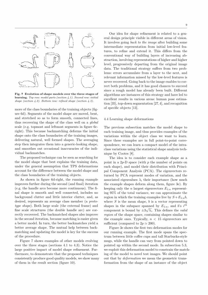
Fig. 7 Evolution of shape models over the three stages oflearning. Top row: model parts (section 4.1). Second row: initialshape (section 4.2). Bottom row: refined shape (section 4.3).

more of the class boundaries of the training objects (fig-

ure 6d). Segments of the model shape are moved, bent,

and stretched so as to form smooth, connected lines,thus recovering the shape of the class well on a global

scale (e.g. topmost and leftmost segments in figure 6c-

right). This because backmatching deforms the initial

shape onto the class boundaries of the training images,delivering natural, well formed shapes. The averaging

step then integrates them into a generic-looking shape,

and smoothes out occasional inaccuracies of the indi-vidual backmatches.

The proposed technique can be seen as searching for

the model shape that best explains the training data,under the general assumption that TPS deformations

account for the difference between the model shape and

the class boundaries of the training objects.

As shown in figure 6d-right, the running example

improves further during the second (and final) iteration

(e.g. the handle arcs become more continuous). The fi-

nal shape is smooth and well connected, includes nobackground clutter and little interior clutter, and, as

desired, represents an average class member (a proto-

type shape). Both large scale (the external frame) andfine scale structures (the double handle arc) are cor-

rectly recovered. The backmatched shapes also improve

in the second iteration, because matching is easier givena better model. In turn, the better backmatches yield a

better average shape. The mutual help between back-

matching and updating the model is key for the success

of the procedure.

Figure 7 shows examples of other models evolving

over the three stages (sections 4.1 to 4.3). Notice the

large positive impact of model shape refinement. Fur-thermore, to demonstrate that the proposed techniques

consistently produce good quality models, we show many

of them in the result section (figure 10).

Our idea for shape refinement is related to a gen-

eral design principle visible in different areas of vision.It involves going back to the image after building some

intermediate representation from initial low-level fea-

tures, to refine and extend it. This differs from theconventional way of building layers of increasing ab-

straction, involving representations of higher and higher

level, progressively departing from the original imagedata. The traditional strategy suffers from two prob-

lems: errors accumulate from a layer to the next, and

relevant information missed by the low-level features is

never recovered. Going back to the image enables to cor-rect both problems, and it has good chances to succeed

since a rough model has already been built. Different

algorithms are instances of this strategy and have led toexcellent results in various areas: human pose estima-

tion [35], top-down segmentation [27,4], and recognition

of specific objects [13].

4.4 Learning shape deformations

The previous subsection matches the model shape to

each training image, and thus provides examples of thevariations within the object class we want to learn.

Since these examples are in full point-to-point corre-

spondence, we can learn a compact model of the intra-class variations using the statistical shape analysis tech-

nique by Cootes [8].

The idea is to consider each example shape as a

point in a 2p-D space (with p the number of points oneach shape), and model their distribution with Princi-

pal Component Analysis (PCA). The eigenvectors re-

turned by PCA represent modes of variation, and theassociated eigenvalues λi their importance (how much

the example shapes deform along them, figure 3e). By

keeping only the n largest eigenvectors E1:n represent-ing 95% of the total variance, we can approximate the

region in which the training examples live by S +E1:nb,

where S is the mean shape, b is a vector representing

shapes in the subspace spanned by E1:n, and b’s ith

component is bound by ±3√

λi. This defines the valid

region of the shape space, containing shapes similar to

the example ones. Typically, n < 15 eigenvectors aresufficient (compared to 2p ≃ 200).

Figure 3e shows the first two deformation modes for

our running example. The first mode spans the spec-trum between little coffee cups and tall Starbucks-style

mugs, while the handle can vary from pointed down to

pointed up within the second mode. In subsection 5.3,

we exploit this deformation model to constrain the match-ing of the model to novel test images. We should point

out that by deformation we mean the geometric trans-

formation from the shape of an instance of the object

10

class to another instance. Although a single mug is not

a rigid object, we need a non-rigid transformation tomap the shape of a mug to that of another mug.

Notice that previous works on these deformation

models require at least the example shapes as input [21],and many also need the point-to-point correspondences [8].

In contrast, we automatically learn shapes, correspon-

dences, and deformations given just images.

5 Object detection

In this section we describe how to localize the bound-

aries of previously unseen object instances in a test im-

age. To this end, we match the shape model learnt inthe previous section to the test image edges. This task

is very challenging, because 1) the image can be exten-

sively cluttered, with the object covering only a small

proportion of its edges (figure 8a-b); and 2) to han-dle intra-class variability, the shape model must be de-

formed into the shape of the particular instance shown

in the test image.We decompose the problem into two stages. We first

obtain rough estimates for location and scale of the

object based on a Hough-style voting scheme (subsec-tion 5.1). This greatly simplifies the subsequent shape

matching, as it approximately lifts three degrees of free-

dom (translation and scale). The estimates are then

used to initialize the non-rigid shape matcher [6] (sub-section 5.2). This combination enables [6] to operate

in cluttered images, and hence allows to localize ob-

ject boundaries. Furthermore, in subsection 5.3, we con-strain the matcher to explore only the region of shape

space spanned by the training examples, thereby ensur-

ing that output shapes are similar to class members.

5.1 Initialization by Hough voting

In subsection 4.1 we have represented the shape of a

class as a set of PAS parts, each with a specific shape, lo-

cation, size, and confidence. Here we match these partsto PAS from the test image, based on their shape de-

scriptors. More precisely, a model part is deemed matched

to an image PAS if their dissimilarity (1) is below athreshold γ (this is the same as used in section 4.1).

Since a pair of matched PAS induces a translation and

scale transformation, each match votes for the presenceof an object instance at a particular location (object

center) and scale (in the same spirit as [27,32,39]).

Votes are weighed by the shape similarity between the

model part and test PAS, the edge strength of the PAS,and the confidence of the part. Local maxima in the

voting space define rough estimates of the location and

scale of candidate object instances (figure 8c).

c d e

a b

Fig. 8 Object detection. (a) A challenging test image and

its edgemap b). The object covers only about 6% of the imagesurface, and only about 1 edgel in 17 belongs to its boundaries.(c) Initialization with a local maximum in Hough space. (d) Out-put shape with unconstrained TPS-RPM. It recovers the object

boundaries well, but on the bottom-right corner, where it is at-tracted by the strong-gradient edgels caused by the shading insidethe mug. (e) Output of the shape-constrained TPS-RPM. The

bottom-right corner is now properly recovered.

The above voting procedure delivers 10 to 40 local

maxima in a typical cluttered image, as the local fea-

tures are not very distinctive on their own. The impor-tant point is that a few tens is far less than the number

of possible location and scales the object could take

in the image, which is in the order of the thousands.Thus, Hough voting acts as a focus of attention mecha-

nism, drastically reducing the problem complexity. We

can now afford to run a full-featured shape matchingalgorithm [6], starting from each of the initializations.

Note that running [6] directly, without initialization,

is likely to fail on very cluttered images, where only a

small minority of edgels are on the boundaries of thetarget object.

5.2 Shape Matching by TPS-RPM

For each initial location l and scale s found by Hough

voting, we obtain a point set V by centering the model

shape on l and rescaling it to s, and a set X whichcontains all image edge points within a larger rectan-

gle of scale 1.8s (figure 8c). This larger rectangle is

designed to contain the whole object, even when s isunder-estimated. Any point outside this rectangle is ig-

nored by the shape matcher.

Given the initialization, we want to put V in cor-

respondence with the subset of X lying on the objectboundary. We estimate the associated non-rigid trans-

formation, and reject image points not corresponding

to any model point with the Thin-Plate Spline Robust

11

Point Matching algorithm (TPS-RPM [6]). In this sub-

section we give a brief summary of TPS-RPM, and werefer to [6] for details.

TPS-RPM matches the two point sets V = {va}a=1..K

and X = {xi}i=1..N by applying a non-rigid TPS map-

ping {d,w} to V (d is the affine component, and w thenon-rigid warp). It estimates both the correspondence

matrix M = {mai} between V and X, and the mapping

{d,w} that minimize an objective function including 1)the distance between points of X and their correspond-

ing points of V after mapping them by the TPS, and 2)

the regularization terms for the affine and warp compo-

nents of the TPS. In addition to the inner K ×N part,M has an extra row and an extra column which allow

to reject points as unmatched.Since neither the correspondence M nor the TPS

mapping {d,w} are known beforehand, TPS-RPM iter-atively alternates between updating M , while keeping{d,w} fixed, and updating the mapping with M fixed.M is a continuous-valued soft-assign matrix, allowingthe algorithm to evolve through a continuous correspon-dence space, rather than jumping around in the spaceof binary matrices (hard correspondence). It is updatedby setting mai as a function of the distance between xi

and va, after mapping by the TPS (details below). Theupdate of the mapping fits a TPS between V and thecurrent estimate Y = {ya}a=1..K of the correspondingpoints. Each point ya in y is a linear combination ofall image points {xi}i=1..N weighted by the soft-assignvalues M(a, i):

ya =N

X

i=1

maixi (6)

The TPS fitting maximizes the proximity between

the points Y and the model points V after TPS map-

ping, under the influence of the regularization terms,which penalize local warpings w and deviations of d

from the identity. Fitting the TPS to V ↔ Y rather

than to V ↔ X, allows to harvest the benefits of man-

taining a full soft-correspondence matrix M .The optimization procedure of TPS-RPM is embed-

ded in a deterministic annealing framework by intro-ducting a temperature parameter T , which decreasesat each iteration. The entries of M are updated by thefollowing equation:

mai =1

Texp

„

(xi − f(va, d, w))T (xi − f(va, d, w))

2T

«

(7)

where f(va, d, w) is the mapping of point va by the TPS{d,w}. The entries of M are then iteratively normalized

to ensure the rows and columns sum to 1 [6]. Since T is

the bandwidth of the Gaussian kernel in equation (7),

as it decreases M becomes less fuzzy, progressively ap-proaching a hard correspondence matrix. At the same

time, the regularization terms of the TPS is given less

weight. Hence, the TPS is rigid in the beginning, and

after iter 1 after iter 8 after iter 12

unconstrained TPS−RPM

TPS−RPM with class−specific shape constraints

Fig. 9 Three iterations of TPS-RPM initialized as in fig-ure 8c. The image points X are shown in red, and the current

shape estimate Y in blue. The green circles have radius pro-portional to the temperature T , and give an indication of therange of potential correspondence considered by M . This is fullyshown by the yellow lines joining all pairs of points with non-

zero mai. Top: unconstrained TPS-RPM. Bottom: TPS-RPMwith the proposed class-specific shape constraints. The two pro-cesses are virtually identical until iteration eight, when the un-

constrained matcher diverges towards interior clutter. The con-strained version instead, sticks to the true object boundary.

gets more and more deformable as the iterations con-

tinue. These two phenomena enable TPS-RPM to find

a good solution even when given a rather poor initial-ization. At first, when the correspondence uncertainty

is high, each ya essentially averages over a wide area of

X around the TPS-mapped point and the TPS is con-strained to near-rigid transformations. This can be seen

as a large T in equation (7) generates similar-valued

mai, which are then averaged by equation (6). As the

iterations continue and the temperature decreases, Mlooks less and less far, and pays increasing attention

to the differences between matching options from X.

Since the uncertainty diminishes, it is safe to let theTPS looser, freer to fit the details of X more accu-

rately. Figure 9 illustrates TPS-RPM on our running

example.

We have extended TPS-RPM by adding two terms

to the objective function: the orientation difference be-

tween corresponding points (minimize), and the edge

strength of matched image points (maximize). In ourexperiments, these extra terms made TPS-RPM more

accurate and stable, i.e. it succeeds even when initial-

ized farther away from the best location and scale.

12

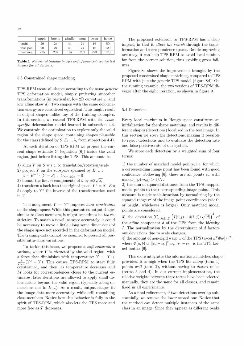
apple bottle giraffe mug swan horse

train 20 24 44 24 16 50

test pos 20 24 43 24 16 120

test neg 215 207 167 207 223 170

Table 1 Number of training images and of positive/negative testimages for all datasets.

5.3 Constrained shape matching

TPS-RPM treats all shapes according to the same generic

TPS deformation model, simply preferring smoother

transformations (in particular, low 2D curvature w, and

low affine skew d). Two shapes with the same deforma-tion energy are considered equivalent. This might result

in output shapes unlike any of the training examples.

In this section, we extend TPS-RPM with the class-

specific deformation model learned in subsection 4.4.

We constrain the optimization to explore only the valid

region of the shape space, containing shapes plausiblefor the class (defined by S,E1:n, λi from subsection 4.4).

At each iteration of TPS-RPM we project the cur-rent shape estimate Y (equation (6)) inside the valid

region, just before fitting the TPS. This amounts to:

1) align Y on S w.r.t. to translation/rotation/scale

2) project Y on the subspace spanned by E1:n :b = E−1 · (Y − S) , b(n+1):2p = 0

3) bound the first n components of b by ±3√

λi

4) transform b back into the original space: Y c = S+E·b5) apply to Y c the inverse of the transformation used

in 1)

The assignment Y ← Y c imposes hard constraints

on the shape space. While this guarantees output shapes

similar to class members, it might sometimes be too re-strictive. To match a novel instance accurately, it could

be necessary to move a little along some dimensions of

the shape space not recorded in the deformation model.The training data cannot be assumed to present all pos-

sible intra-class variations.

To tackle this issue, we propose a soft-constrained

variant, where Y is attracted by the valid region, with

a force that diminishes with temperature: Y ← Y +T

Tinit(Y c − Y ). This causes TPS-RPM to start fully

constrained, and then, as temperature decreases and

M looks for correspondences closer to the current es-timates, later iterations are allowed to apply small de-

formations beyond the valid region (typically along di-

mensions not in E1:n). As a result, output shapes fit

the image data more accurately, while still resemblingclass members. Notice how this behavior is fully in the

spirit of TPS-RPM, which also lets the TPS more and

more free as T decreases.

The proposed extension to TPS-RPM has a deep

impact, in that it alters the search through the trans-formation and correspondence spaces. Beside improving

accuracy, it can help TPS-RPM to avoid local minima

far from the correct solution, thus avoiding gross fail-ures.

Figure 8e shows the improvement brought by theproposed constrained shape matching, compared to TPS-

RPM with just the generic TPS model (figure 8d). On

the running example, the two versions of TPS-RPM di-verge after the eight iteration, as shown in figure 9.

5.4 Detections

Every local maximum in Hough space constitutes an

initialization for the shape matching, and results in dif-ferent shapes (detections) localized in the test image. In

this section we score the detections, making it possible

to reject detections and to evaluate the detection rate

and false-positive rate of our system.

We score each detection by a weighted sum of fourterms:

1) the number of matched model points, i.e. for whicha corresponding image point has been found with good

confidence. Following [6], these are all points va with

maxi=1..N (mai) > 1/N .2) the sum of squared distances from the TPS-mapped

model points to their corresponding image points. This

measure is made scale-invariant by normalizing by thesquared range r2 of the image point coordinates (width

or height, whichever is larger). Only matched model

points are considered.

3) the deviation∑

i,j∈[1,2]

(

I(i, j) − d(i, j)/√

|d|)2

of

the affine component d of the TPS from the identity

I. The normalization by the determinant of d factors

out deviations due to scale changes.

4) the amount of non-rigid warp w of the TPS trace(wT Φw)/r2,where Φ(a, b) ∝ ||va−vb||2 log ||va−vb|| is the TPS ker-

nel matrix [6].

This score integrates the information a matched shape

provides. It is high when the TPS fits many (term 1)

points well (term 2), without having to distort much(terms 3 and 4). In our current implementation, the

relative weights between these terms have been selected

manually, they are the same for all classes, and remainfixed in all experiments.

As a final refinement, if two detections overlap sub-stantially, we remove the lower scored one. Notice that

the method can detect multiple instances of the same

class in an image. Since they appear as different peaks

13

in the Hough voting space, they result in separate de-

tections.

6 Experiments

We present an extensive evaluation involving six di-

verse object classes from two existing datasets [14,25].

After introducing the datasets in the next subsection,

we evaluate our approach for learning shape models insubsection 6.2. The ability to localize objects in novel

images, both in terms of bounding-boxes and bound-

aries, is measured in subsection 6.3. All experimentsare run with the same parameters (no class-specific nor

dataset-specific tuning is applied).

6.1 Datasets and protocol

ETHZ shape classes [14].This dataset features five

diverse classes (bottles, swans, mugs, giraffes, apple-logos) and contains a total of 255 images collected from

the web. It is highly challenging, as the objects appear

in a wide range of scales, there is considerable intra-class shape variation, and many images are severely

cluttered, with objects comprising only a fraction of

the total image area (figures 13 and 18).

For each class, we learn 5 models, each from a dif-ferent random sample containing half of the available

images (there are 40 for apple-logos, 48 for bottles, 87

for giraffes, 48 for mugs and 32 for swans). Learningmodels from different training sets allows to evaluate

the stability of the proposed learning technique (sub-

section 6.2). Notice that our method does not require

negative training images i.e. images not containing anyinstance of the class.

The test set for a model consists of all other im-

ages in the dataset. Since this includes about 200 nega-tive images, it allows to properly estimate false-positive

rates. Table 1 gives an overview of the composition of

all training and testing sets. We refer to learning andtesting on a particular split of the images as a trial.

INRIA horses [25].This challenging dataset consistsof 170 images with one or more horses viewed from the

side and 170 images without horses. Horses appear at

several scales, and against cluttered backgrounds.

We train 5 models, each from a different randomsubset of 50 horse images. For each model, the remain-

ing 120 horse images and all 170 negative images are

used for testing, see table 1.

6.2 Learning shape models

Evaluation measures. We assess the performance ofthe learning procedure of section 4 in terms of how accu-

rately it recovers the true class boundaries of the train-

ing instances. For this evaluation, we have manually

annotated the boundaries of all object instances in theETHZ shape classes dataset. We will present results for

all of these five classes.

Let Bgt be the ground-truth boundaries, and Bmodel

the backmatched shapes output by the model shape re-

finement algorithm of subsection 4.3. The accuracy oflearning is quantified by two measures. Coverage is the

percentage of points from Bgt closer than a threshold t

from any point of Bmodel. We set t to 4% of the diago-nal of the bounding-box of Bgt. Conversely, precision is

the percentage of Bmodel points closer than t from any

point of Bgt. The measures are complementary. Cov-erage captures how much of the object boundary has

been recovered by the algorithm, whereas precision re-

ports how much of the algorithm’s output lies on the

object boundaries.

Models from the full algorithm. Table 2 shows

coverage and precision averaged over training instances

and trials, for the complete learning procedure describedin section 4. With the exception of giraffes, the pro-

posed method achieves very high coverage (above 90%),

demonstrating its ability to discover which contour pointsbelong to the class boundaries. The precision of apple-

logos and bottles is also excellent, thanks to the clean

prototype shapes learned by our approach (figure 10).Interestingly, the precision of mugs is somewhat lower,

because the learned shapes include a detail not present

in the ground-truth annotations, although it is arguably

part of the class boundaries: the inner half of the open-ing on top of the mug. A similar phenomenon penalizes

the precision of swans, where our method sometimes in-

cludes a few water waves in the model. Although theyare not part of the swan boundaries, waves acciden-

tally occurring at a similar position over many train-

ing images are picked up by the algorithm. A largertraining set might lead to the suppression of such arti-

facts, as waves have less chances of accumulating acci-

dentally (we only used 16 images). The modeling per-

formance for giraffes is lower, due to the extremely clut-tered edgemaps arising from their natural environment,

and to the camouflage texture which tends to break

edges along the body outlines (figure 11).

Models without assembling the initial shape. We

experiment with a simpler scheme for learning shape

models by skipping the procedure for assembling the

14

apple bottle giraffe mug swan

Full system 90.2 / 90.6 96.2 / 92.7 70.8 / 74.3 93.9 / 83.6 90.0 / 80.0

No assembly 91.2 / 92.7 96.8 / 88.1 70.0 / 72.6 92.6 / 82.9 89.4 / 79.2

Table 2 Accuracy of learned models. Each entry is the average coverage/precision over trials and training instances.

Fig. 10 Learned shape models for ETHZ Shape Classes (threeout of total five per class). Top three rows: models learnt usingthe full method presented in section 4. Last row: models learnt

using the same training images used in row 3, but skipping theprocedure for assembling the initial shape (subsection 4.2; doneonly for ETHZ shape classes).

initial shape (section 4.2). An alternative initial shape

can be obtained directly from the COP model (sec-

tion 4.1) by picking, for each part, the occurrence clos-

est to the peak in the voting space corresponding tothe part (as in section 4.1). This initial shape can then

be passed on to the shape refinement stage as usual

(section 4.3).

For each object class and trial we have rerun thelearning algorithm without the assembly stage, but oth-

erwise keeping identical conditions (including using ex-

actly the same training images). Many of the result-ing prototype shapes are moderately worse than those

obtained using the full learning scheme (figure 10 bot-

tom row). However, the lower model quality only re-sults in slightly lower average coverage/accuracy values

(table 2). These results suggest that while the initial as-

sembly stage does help getting better models, it is not

a crucial step, and that the shape refinement stage ofsection 4.3 is robust to large amounts of noise, and de-

livers good models even when starting from poor initial

shapes.

Fig. 11 A typical edgemap for a Giraffe training window is verycluttered and edges are broken along the animal’s outline, makingit difficult to learn clean models.

6.3 Object detection

Detection up to a bounding-box. We first evalu-

ate the ability of the object detection procedure of sec-tion 5 to localize objects in cluttered test images up

to a bounding-box (i.e. the traditional detection task

commonly defined in the literature).

Figure 12 reports detection-rate against the num-

ber of false-positives averaged over all 255 test images(FPPI) and averaged over the 5 trials. As discussed

above, this includes mostly negative images. We adopt

the strict standards of the PASCAL Challenge criterion(dashed lines in the plots): a detection is counted as cor-

rect only if the intersection-over-union ratio (IoU) with

the ground-truth bounding-box is greater than 50%. All

other detections are counted as false-positives. In orderto compare to [14,16], we also report results under their

somewhat softer criterion: a detection is counted as cor-

rect if its bounding-box overlaps more than 20% withthe ground-truth one, and vice-versa (we refer to this

criterion as 20%-IoU).

As the plots show, our method performs well on all

classes but giraffes, with detections-rates around 80%

at the moderate false-positive rate of 0.4 FPPI (thisis the reference point for all comparisons). The lower

performance on giraffes is mainly due to the difficulty

of building shape models from their extremely noisyedge maps.

It is interesting to compare against the detection

performance obtained by the Hough voting stage alone

(subsection 5.1), without the shape matcher on top

(subsections 5.2, 5.3). The full system performs sub-stantially better: the difference under PASCAL crite-

rion is about +30% averaged over all classes. This shows

the benefit of treating object detection fully as a shape

15

0 0.2 0.4 0.6 0.8 1 1.2 1.40

0.1

0.2

0.3

0.4

0.5

0.6

0.7

0.8

0.9

1

False−positives per image

Det

ectio

n ra

te

INRIA Horses

0 0.2 0.4 0.6 0.8 1 1.2 1.40

0.1

0.2

0.3

0.4

0.5

0.6

0.7

0.8

0.9

1

False−positives per image

De

tect

ion

ra

te

Swans

0 0.2 0.4 0.6 0.8 1 1.2 1.40

0.1

0.2

0.3

0.4

0.5

0.6

0.7

0.8

0.9

1

False−positives per image

De

tect

ion

ra

te

Apple logos

0 0.2 0.4 0.6 0.8 1 1.2 1.40

0.1

0.2

0.3

0.4

0.5

0.6

0.7

0.8

0.9

1

False−positives per imageD

etec

tion

rate

Bottles

0 0.2 0.4 0.6 0.8 1 1.2 1.40

0.1

0.2

0.3

0.4

0.5

0.6

0.7

0.8

0.9

1

False−positives per image

Det

ectio

n ra

te

Giraffes

0 0.2 0.4 0.6 0.8 1 1.2 1.40

0.1

0.2

0.3

0.4

0.5

0.6

0.7

0.8

0.9

1

False−positives per image

De

tect

ion

ra

te

Mugs

Ferrari et al. PAMI 08 (PASCAL)

Full system (20% IoU)

Full system (PASCAL)

Hough only (PASCAL)

Ferrari et al. PAMI 08 (20% IoU)

Fig. 12 Object detection performance (models learnt from real images). Each plot shows five curves: the full system evaluated under

the PASCAL criterion for a correct detection (dashed, thick, red), the full system under the 20%-IoU criterion (solid, thick, red), the

Hough voting stage alone under PASCAL (dashed, thin, blue), [16] under 20%-IoU (solid, thin, green) and under PASCAL (dashed,thin, green). The curve for the full system under PASCAL in the apple-logo plot is identical to the curve for 20%-IoU.

matching task, rather than simply matching local fea-

tures, which is one of the principal points of this paper.Moreover, the shape matching stage also makes it possi-

ble to localize complete object boundaries, rather than

just bounding-boxes (figure 13).

The difference between the curves under the PAS-

CAL criterion and the 20%-IoU criterion of [14,16] is

small for apple-logos, bottles, mugs and swans (0%,−1.6%, −3.6%, −4.9%), indicating that most detec-

tions have accurate bounding-boxes. For horses and gi-

raffes the decrease is more significant (−18.1%,−14.1%),

because the legs of the animals are harder to detectand cause the bounding-box to shift along the body.

On average over all classes, our method achieves 78.1%

detection-rate at 0.4 FPPI under 20%-IoU and 71.1%under PASCAL. The corresponding standard-deviation

over trials, averaged over classes, is 8.1% under 20%-

IoU and 8.0% under PASCAL (this variation is due todifferent trials having different training and test sets).

For reference, the plots also show the performance

of [16] on the same datasets, using the same numberof training and test images. An exact comparison is

not possible, as [16] reports result based on only one

training/testing split, whereas we average over 5 ran-

dom splits. Under the rather permissive 20%-IoU crite-rion, [16] performs a little better than our method on

average over all classes. Under the strict PASCAL cri-

terion instead, our method performs substantially bet-

ter than [16] on two classes (apple-logos, swans), mod-

erately worse on two (bottles, horses), and about thesame on two (mugs, giraffes), thanks to the higher ac-

curacy of the detected bounding-boxes. Averaged over

all classes, under PASCAL our method reaches 71.1%

detection-rate at 0.4 FPPI, comparing well against the68.5% of [16]. Note how our results are achieved with-

out the beneficial discriminative learning of [16], where

a SVM learns which PAS types at which relative loca-tion within the training bounding-box best discriminate

between instances of the class and background image

windows. Our method instead trains only from positiveexamples.

For clarity and reference for comparison by future

works, we summarize here our results on the ETHZShape Classes alone (without INRIA horses). Under

PASCAL, averaged over all 5 trials and 5 classes, our

method achieves 72.0%/67.2% detection-rate at 0.4/0.3FPPI respectively. Under 20%-IoU, it achieves 76.8%/71.5%

detection-rate at 0.4/0.3 FPPI.

After our results were first published [15], Fritz andSchiele [20] presented an approach based on topic mod-

els and a dense gradient histogram representation of im-

age windows (no explicit shapes). They report results

on the ETHZ Shape Classes dataset (i.e. no horses), us-ing the same protocol (5 random trials). Their method

achieves 84.8% averaged over classes, improving over

our 76.8% (both at 0.4 FPPI and under 20%-IoU).

16

Fig. 13 Example detections (models learnt from images). Notice the large scale variations (especially in apple-logos, swans), the intra-

category shape variability (especially in swans, giraffes), and the extensive clutter (especially in giraffes, mugs). The method worksfor photographs as well as paintings (first swan, last bottle). Two bottle cases show also false-positives. In the first two horse images,the horizontal line below the horses’ legs is part of the model and represents the ground. Interestingly, the ground line systematicallyreoccurs over the training images for that model and gets learned along with the horse.

17

Fig. 15 Learned shape models for INRIA horses (three out oftotal five), using the method presented in section 4.

Beyond the above quantiative evaluation, the method

presented in this paper offers two important advantages

over both [16] and [20]. It localizes object boundaries,rather than just bounding-boxes, and can also detect

objects starting from a single hand-drawing as a model

(see below).

Localizing object boundaries. The most interest-

ing feature of our approach is the ability to localizeobject boundaries in novel test images. This is shown

by several examples in figure 13, where the method

succeeds in spite of extensive clutter, a large range ofscales, and intra-class variability (typical failure cases

are discussed in figure 16). In the following we quantify

how accurately the output shapes match the true ob-ject boundaries. We use the coverage and precision mea-

sures defined above. In the present context, coverage is

the percentage of ground-truth boundary points recov-

ered by the method and precision is the percentage ofoutput points that lie on the ground-truth boundaries.

All shape models used in these experiments have been

learned from real images, as discussed before. Severalmodels for each object class are shown in figures 10 and

15.

Table 3 shows coverage and precision averaged overtrials and correct detections at 0.4 FPPI. Coverage ranges

in 78 − 92% for all classes but giraffes, demonstrating

that most of the true boundaries have been successfully

detected. Moreover, precision values are similar, indi-cating that the method returns only a small proportion

of points outside the true boundaries. Performance is

lower for giraffes, due to the more noisy models anddifficult edgemaps derived from the test images.

Although it uses the same evaluation metric, the ex-

periment carried out at training time in subsection 6.2differs substantially from the present one, because at

testing time the system is not given ground-truth bounding-

boxes. In spite of the important additional challengeof having to determine the object’s location and scale

in the image, the coverage/precision scores in table 3

are only moderately lower than those achieved during

training (table 3; the average difference in coverage andprecision is 7.1% and 2.1% respectively). This demon-

strates that our detection approach is highly robust to

clutter.

As a baseline, table 3 also reports coverage/precision

results when using the ground-truth bounding-boxes as

shapes. The purpose of this experiment is to compare

the accuracy of our method to the maximal accuracy

that can be achieved when localizing objects up to abounding-box. As the table clearly shows, the shapes

returned by our method are substantially more accurate

than the best bounding-box, thereby proving one of theprincipal points of this paper. While the average differ-

ence is about 35%, it is interesting to observe how the

difference is greater for less rectangular objects (swans,

giraffes, apple-logos) than for bottles and mugs. Noticealso how our method is much more accurate than the

ground-truth bounding-box even for giraffes, the class

where it performs the worst.

Finally, we investigate the impact of the constrainedshape matching technique proposed in subsection 5.3,

by re-running the experiment without it, simply rely-

ing on the deformation model implicit in the thin-platespline formulation (table 3, second row). The cover-

age/precision values are very similar to those obtained

through constrained shape matching. The reason is thatmost cases are either already solved accurately without

learned deformation models, or they do not improve

when using them because the low accuracy is due to

particularly bad edgemaps. In practice, the differencemade by constrained shape matching is visible in about

one case every six, and it is localized to a relatively

small region of the shape (figure 14). The combina-tion of these two factors explains why constrained shape

matching appears to make little quantitative difference,

although in many cases the localized boundaries im-prove visibly.

Detection from hand-drawn models. A useful char-acteristic of the proposed approach is that, unlike most

existing object detection methods, it can take either a

hand-drawing as a model, or learn it from real images.

When given a hand-drawing as a model, our approachdoes not perform the learning stage, and naturally falls

back to the functionality of pure shape matchers which

takes a clean shape as input (e.g. the recent works [14,38], which support matching to cluttered test images).

In this case, the modeling stage simply decomposes

the hand-drawing into PAS. Object detection then usesthese PAS for the Hough voting stage, and the hand-

drawing itself for the shape matching stage. As no defor-

mation model can be learnt from a single example, our

method naturally switches to the standard deformationmodel implicit in the Thin-Plane Spline formulation.

Figure 17 compares our method to [14] using their

exact setup, i.e. with a single hand-drawing per class as

model and all 255 images of the ETHZ shape classes as

18

shape constraineddefault TPSshape constraineddefault TPSFig. 14 (left) typical improvement brought by constrained shape matching over simply using the TPS deformation model. As theimprovement is often a refinement of a local portion of the shape (the swan’s tail in this case), the numerical differences in theevaluation measures is only modest (in this case less than 1%). (right) an infrequent case, where constrained shape matching fixes

the entirely wrong solution delivered by standard matching. The numerical difference in such cases is noticeable (about 6%).

apple bottle giraffe mug swan

Full system 91.6 / 93.9 83.6 / 84.5 68.5 / 77.3 84.4 / 77.6 77.7 / 77.2

No learned deform 91.3 / 93.6 82.7 / 84.2 68.4 / 77.7 83.2 / 75.7 78.4 / 77.0

Ground-truth BB 42.5 / 40.8 71.2 / 67.7 26.7 / 29.8 55.1 / 62.3 36.8 / 39.3

Table 3 Accuracy of localized object boundaries at test time. Each entry is the average coverage/precision over trials andcorrect detections at 0.4 FPPI.

a b c

Fig. 16 Example failed detections (models learnt from images). (a) A typical case. A good match to the image edges is

found, but at the wrong scale. Our system has no bias for any particular scale. (b) Another typical case. Failure is due to an extremelycluttered edge-map. The neck is correctly matched, and gives rise to a peak in the Hough voting space (section 5.1). However, thesubsequent deformable matching stage (section 5.2) is attracted by the high contrast waves in the background. (c) An infrequent case.

Failure is due to a poor shape model (right, this the worst of the 30 models we have learned).

test set. Therefore, the test set for each class containsmostly images not containing any instance of the class,

which supports the proper estimatation of FPPI. Our

method performs better than [14] on all 5 classes, espe-

cially in the low FPPI range, and substantially outper-forms the oriented chamfer matching baseline (details

in [14]). Averaged over classes, our method achieves

85.3%/82.4% detection-rate at 0.4/0.3 FPPI respectively,compared to 81.5%/70.5% of [14] (all results under 20%-

IoU). As one reason for this improvement, our method

is more robust because it does not need the test imageto contain long chains of contour segments around the

object.

After our results were first published [15], two worksreported even better performance. Ravishankar et al. [36]

achieve 95.2% at 0.4 FPPI. Zhu et al. [45] reports 0.21

FPPI at 85.3% detection-rate (ours). Note this is the

opposite of the usual way, reporting detection-rate ata reference FPPI [14–16,20,36]). All results are under

20%-IoU and averaged over classes. As part of the rea-

son for the high performance, Ravishankar et al. [36]

propose a sophisticated scoring method which allowsto reliably reject false-positives, while the method of

Zhu et al. [45] relies on their algorithm [46] to find

long salient contours, effectively removing many clut-

ter edgels before the object detector runs. An interest-ing avenue for further research is incorporating these

successful elements in our framework.

Beside this quantitative evaluation, the main ad-

vantage of our approach over [14,36,45] is that it canalso train from real images (which is the main topic

of this paper). Moreover, compared to [14], it supports

branching and self-intersecting input shapes.

Interestingly, in our system hand-drawings lead to

moderately better detection results than when learningmodels from images. This is less suprising when consid-

ering that hand-drawings are essentially the prototype

shapes the system tries to learn.

19

0 0.2 0.4 0.6 0.8 1 1.2 1.40

0.1

0.2

0.3

0.4

0.5

0.6

0.7

0.8

0.9

1

False−positives per image

De

tect

ion

ra

te

Apple logos

Chamfer matchingFerrari et al. ECCV 2006Our method

0 0.2 0.4 0.6 0.8 1 1.2 1.40

0.1

0.2

0.3

0.4

0.5

0.6

0.7

0.8

0.9

1

False−positives per image

De

tect

ion

ra

te

Swans

0 0.2 0.4 0.6 0.8 1 1.2 1.40

0.1

0.2

0.3

0.4

0.5

0.6

0.7

0.8

0.9

1

False−positives per image

De

tect

ion

ra

te

Mugs

0 0.2 0.4 0.6 0.8 1 1.2 1.40

0.1

0.2

0.3

0.4

0.5

0.6

0.7

0.8

0.9

1

False−positives per imageD

ete

ctio

n r

ate

Bottles

0 0.2 0.4 0.6 0.8 1 1.2 1.40

0.1

0.2

0.3

0.4

0.5

0.6

0.7

0.8

0.9

1

False−positives per image

De

tect

ion

ra

te

Giraffes

Fig. 17 Object detection performance (hand-drawn models). To facilitate comparison, all curves have been computed usingthe 20%-IoU criterion of [14].

Fig. 18 Detection from hand-drawn models. Top: four of the five models from [14]. There is just one example per object class.Bottom: example detections delivered by our shape matching procedure, using these hand-drawings as models.

7 Conclusions and future work

We have proposed an approach for learning class-specificexplicit shape models from images annotated by bounding-

boxes, and localizing the boundaries of novel class in-

stances in the presence of extensive clutter, scale changes,

and intra-class variability. In addition, the approachoperates effectively also when given hand-drawings as

models. The ability to input both images and hand-

drawings as training data is a consequence of the basicdesign of our approach, which attempts to bridge the

gap between shape matching and object class detection.

The presented approach can be extended in several

ways. First, the training stage models only positive ex-

amples. This could be extended by learning a classi-

fier to distinguish between positive and negative exam-

ples, which might reduce false positives. One possibilitycould be to train both our shape models and the dis-

criminative models of [16]. At detection time, we could

then use the bounding-box delivered by [16] to initial-ize shape matching based on our models. Moreover, the

discriminative power of the representation could be im-

proved by using appearance features in addition to im-

age contours. Finally, in this paper we have assumedthat all observed differences in the shape of the training

examples originate from intra-class variation, and not

from viewpoint changes. It would be interesting to add

20

a stage to automatically group objects by viewpoint,

and learn separate shape models.

References

1. R. Basri, L. Costa, D. Geiger, and D. Jacobs, Determiningthe Similarity of Deformable Shapes, Vision Research, vol. 38,

pp. 2365-2385, 1998.

2. A. Berg, T. Berg and J. Malik, Shape Matching and Ob-ject Recognition using Low Distortion Correspondence, CVPR,2005.

3. S. Belongie and J. Malik, Shape Matching and Object Recog-

nition using Shape Contexts, PAMI, 24(4):509-522, 2002.

4. E. Borenstein and S. Ullman, Class-Specific, Top-Down Seg-mentation, ECCV, 2002.

5. I. Biederman, Recognition-by-components: A theory of human

image understanding, Psychological Review, 94(2):115-147.

6. H. Chui and A. Rangarajan, A new point matching algorithmfor non-rigid registration, CVIU, 89(2-3):114-141, 2003.

7. O. Chum and A. Zisserman, An Exemplar Model for Learning

Object Classes, CVPR, 2007.

8. T. Cootes, C. Taylor, D. Cooper, and J. Graham, Active ShapeModels: Their Training and Application, CVIU, 61(1):38-59,1995.

9. T. Cootes, An Introduction to Active Shape Models, 2000.

10. D. Cremers, T. Kohlberger, and C. Schnorr, Nonlinear ShapeStatistics in Mumford-Shah Based Segmentation, ECCV, 2002.

11. N. Dalal and B. Triggs, Histograms of Oriented Gradientsfor Human Detection, CVPR, 2005.

12. G. Elidan, G. Heitz, D. Koller, Learning Object Shape: From

Drawings to Images, CVPR, 2006.

13. V. Ferrari, T. Tuytelaars, and L. van Gool, SimultaneousObject Recognition and Segmentation by Image Exploration,ECCV, 2004.

14. V. Ferrari, T. Tuytelaars, and L. Van Gool, Object Detectionwith Contour Segment Networks, ECCV, 2006.

15. V. Ferrari, F. Jurie, and C. Schmid, Accurate Object De-tection with Deformable Shape Models Learnt from Images,

CVPR, 2007.

16. V. Ferrari, L. Fevrier, F. Jurie, and C. Schmid, Groupsof Adjacent Contour Segments for Object Detection, PAMI,(30)1:36-51, 2008.

17. P. Felzenswalb, Representation and Detection of DeformableShapes, PAMI, 27(2):208-220, 2005.

18. R. Fergus, P. Perona, and A. Zisserman, Object Class Recog-nition by Unsupervised Scale-invariant Learning, CVPR, 2003.

19. M. Fritz and B. Schiele, Towards Unsupervised Discovery of

Visual Categories, DAGM, 2006.

20. M. Fritz and B. Schiele, Decomposition, discovery and de-tection of visual categories using topic models, CVPR, 2008.

21. A. Hill and C. Taylor, A Method of Non-Rigid Correspon-

dence for Automatic Landmark Identification, BMVC, 1996.

22. D. Gavrila, Multi-Feature Hierarchical Template MatchingUsing Distance Transforms, ICPR, 1998.

23. Y. Gdalyahu and D. Weinshall, Flexible Syntactic Match-

ing of Curves and Its Application to Automatic HierarchicalClassification of Silhouettes, PAMI, 21(12):1312-1328, 1999.

24. S. Gold and A. Rangarajan, Graduated Assignment Algo-rithm for Graph Matching, PAMI, 18(4):377-388, 1996.

25. F. Jurie and C. Schmid, Scale-invariant Shape Features for

Recognition of Object Categories, CVPR, 2004.

26. Y. Lamdan, J. Schwartz, and H. Wolfson, Affine Invari-ant Model-based Object Recognition, IEEE Transactions onRobotics and Automation, 6(5):578-589, 1990.

27. B. Leibe and B. Schiele, Scale-Invariant Object Categoriza-tion using a Scale-Adaptive Mean-Shift Search, DAGM, 2004.

28. M. Leordeanu, M. Hebert, and R. Sukthankar, Beyond Local

Appearance: Category Recognition from Pairwise Interactionsof Simple Features, CVPR, 2007.

29. D. Martin, C. Fowlkes and J. Malik, Learning to detect nat-

ural image boundaries using local brightness, color, and texturecues, PAMI, 26(5):530-549, 2004.

30. D. Marr and H.K. Nishihara, Representation and Recog-nition of the Spatial Organization of Three-DimensionalShapes, Proc. Royal Soc. London, Series B, Biological Sciences,(200):269-294, 1978.

31. F. Mokhtarian and A. Mackworth, Scale-based Descrip-tion and Recognition of Planar Curves and Two-dimensionalShapes, PAMI, 8(1):34-43, 1986.

32. A. Opelt, A. Pinz, and A. Zisserman, A Boundary-Fragment-Model for Object Detection, ECCV, 2006.

33. A. Pentland, A.; Sclaroff, S., Closed-form solutions for phys-ically based shape modeling and recognition, PAMI, 13(7):715-729, 1991.

34. T. Quack, V. Ferrari, B. Leibe, and L. Van Gool, Efficient

Mining of Frequent and Distinctive Feature Configurations,ICCV, 2007.

35. D. Ramanan, Learning to parse images of articulated bodies,NIPS, 2006.

36. S. Ravishankar, A. Jain, and A. Mittal, Multi-stage ContourBased Detection of Deformable Objects, ECCV, 2008.

37. T. Sebastian, P. Klein, and B. Kimia, Recognition of Shapes

by Editing Their Shock Graphs, PAMI, 26(5):550-571, 2004.38. J. Schwartz and P. Felzenszwalb, Hierarchical Matching of

Deformable Shapes, CVPR, 2007.39. J. Shotton, A. Blake, and R. Cipolla, Contour-Based Learn-

ing for Object Detection, ICCV, 2005.40. A. Torralba, K. Murphy, and W. Freeman, Sharing Features:

Efficient Boosting Procedures for Multiclass Object Detection,CVPR, 2004.

41. D. Sharvit, J. Chan, H. Tek, B Kimia, Symmetry-BasedIndexing of Image Databases, IEEE Workshop on Content-Based Access of Image and Video Libraries, 1998.

42. S. Ullman, Aligning pictoral descriptions: An approach toobject recognition, Cognition, 32(3):193-254, 1989.

43. J. Winn and N. Jojic, LOCUS: Learning Object Classes withUnsupervised Segmentation, ICCV, 2005.

44. J. Winn and J. Shotton, The Layout Consistent RandomField for Recognizing and Segmenting Partially Occluded Ob-jects, CVPR, 2006.

45. Q. Zhu, L. Wang, Y. Wu, and J. Shi, Contour Context Se-lection for Object Detection: A Set-to-Set Contour MatchingApproach, ECCV, 2008.

46. Q. Zhu, G. Song, and J. Shi, Untangling cycles for contour

grouping, ICCV, 2007.