from images to shape models for object detection
TRANSCRIPT

Int J Comput Vis (2010) 87: 284–303DOI 10.1007/s11263-009-0270-9
From Images to Shape Models for Object Detection
Vittorio Ferrari · Frederic Jurie · Cordelia Schmid
Received: 23 December 2008 / Accepted: 1 July 2009 / Published online: 17 July 2009© Springer Science+Business Media, LLC 2009
Abstract We present an object class detection approachwhich fully integrates the complementary strengths offeredby shape matchers. Like an object detector, it can learn classmodels directly from images, and can localize novel in-stances in the presence of intra-class variations, clutter, andscale changes. Like a shape matcher, it finds the boundariesof objects, rather than just their bounding-boxes. This isachieved by a novel technique for learning a shape model ofan object class given images of example instances. Further-more, we also integrate Hough-style voting with a non-rigidpoint matching algorithm to localize the model in clutteredimages. As demonstrated by an extensive evaluation, ourmethod can localize object boundaries accurately and doesnot need segmented examples for training (only bounding-boxes).
Keywords Object class detection · Learning categorymodels · Local contour features · Shape matching
This research was supported by the EADS foundation, INRIA, CNRS,and SNSF. V. Ferrari was funded by a fellowship of the EADSfoundation and by SNSF.
V. Ferrari (�)ETH Zurich, Zurich, Switzerlande-mail: [email protected]
F. JurieUniversity of Caen, Caen, Francee-mail: [email protected]
C. SchmidINRIA Grenoble, Grenoble, Francee-mail: [email protected]
1 Introduction
In the last few years, the problem of learning object classmodels and localizing previously unseen instances in novelimages has received a lot of attention. While many methodsuse local image patches as basic features (Fergus et al. 2003;Leibe and Schiele 2004; Torralba et al. 2004; Winn andShotton 2006), recently several approaches based on con-tour features have been proposed (Berg et al. 2005; Ferrariet al. 2006, 2008; Jurie and Schmid 2004; Leordeanu et al.2007; Opelt et al. 2006; Shotton et al. 2005). These are bet-ter suited to represent objects defined by their shape, such asmugs and horses. Most of the methods that train without an-notated object segmentations can localize objects in test im-ages only up to a bounding-box, rather than delineating theiroutlines. We believe the main reason lies in the nature ofthe proposed models, and in the difficulty of learning themfrom real images, as opposed to hand-segmented shapes(Cootes et al. 1995; Elidan et al. 2006; Hill and Taylor 1996;Sebastian et al. 2004). The models are typically composed ofrather sparse collections of contour fragments with a looselayer of spatial organization on top (Ferrari et al. 2008;Jurie and Schmid 2004; Opelt et al. 2006; Shotton et al.2005). A few authors even go to the extreme end of us-ing individual edgels as modeling units (Berg et al. 2005;Leordeanu et al. 2007). In contrast, an explicit shape modelformed by continuous connected curves completely cover-ing the object outlines is more desirable, as it would natu-rally support boundary-level localization in test images.
In order to achieve this goal, we propose an approachwhich bridges the gap between shape matching and objectdetection. Classic non-rigid shape matchers (Belongie andMalik 2002; Chui and Rangarajan 2003; Cootes et al. 1995;Sebastian et al. 2004) produce point-to-point correspon-dences, but need clean pre-segmented shapes as models. In

Int J Comput Vis (2010) 87: 284–303 285
Fig. 1 Example object detections returned by our approach (see alsoFig. 13)
contrast, we propose a method that can learn complete shapemodels directly from images. Moreover, it can automaticallymatch the learned model to cluttered test images, therebylocalizing novel class instances up to their boundaries (asopposed to a bounding-box).
The main contribution of this paper is a technique forlearning the prototypical shape of an object class as wellas a statistical model of intra-class deformations, given im-age windows containing training instances (Fig. 3a; no pre-segmented shapes are needed). The challenge is to deter-mine which contour points belong to the class boundaries,while discarding background and details specific to individ-ual instances (e.g. mug labels). Note how these typicallyform the majority of points, yielding a poor signal-to-noiseratio. The task is further complicated by intra-class variabil-ity: the shape of the object boundary varies across instances.
As additional contributions, we extend the non-rigidshape matcher of Chui and Rangarajan (2003) in twoways. First, we extend it to operate in cluttered test im-ages, by deriving an automatic initialization for the lo-cation and scale of the object from a Hough-style vot-ing scheme (Leibe and Schiele 2004; Opelt et al. 2006;Shotton et al. 2005) (instead of the manual initializationthat would otherwise be necessary). This enables to matchthe learned shape model even to severely cluttered images,where the object boundaries cover only a small fraction ofthe contour points (Figs. 1 and 13). As a second exten-sion, we constrain the shape matcher (Chui and Rangarajan2003) to only search over transformations compatible withthe learned, class-specific deformation model. This ensuresoutput shapes similar to class members, improves accuracy,and helps avoiding local minima.
These contributions result in a powerful system, capableof detecting novel class instances and localizing their bound-aries in cluttered images, while training from objects anno-tated only with bounding-boxes.
After reviewing related work (Sect. 2) and the local con-tour features used in our approach (Sect. 3), we present ourshape learning method in Sect. 4, and the scheme for local-izing objects in test images in Sect. 5. Section 6 reports ex-tensive experiments. We evaluate the quality of the learnedmodels and quantify localization performance at test time in
terms of accuracy of the detected object boundaries. We alsocompare to previous works for object localization with train-ing on real images (Ferrari et al. 2008) and hand-drawings(Ferrari et al. 2006). A preliminary version of this work waspublished at CVPR 2007 (Ferrari et al. 2007).
2 Related Works
As there exists a large body of work on shape representa-tions for recognition (Basri et al. 1998; Belongie and Ma-lik 2002; Cootes et al. 1995; Felzenswalb 2005; Ferrari etal. 2008; Gdalyahu and Weinshall 1999; Gold and Rangara-jan 1996; Leordeanu et al. 2007; Sebastian et al. 2004),we briefly review in the following only the most importantworks relevant to this paper, i.e. on shape description andmatching for modeling, recognition, and localization of ob-ject classes.
Several earlier works for shape description are based onsilhouettes (Mokhtarian and Mackworth 1986; Sharvit et al.1998). Yet, silhouettes are limited because they ignore in-ternal contours and are difficult to extract from clutteredimages as noted by Belongie and Malik (2002). Therefore,more recent works represent shapes as loose collections of2D points (Cootes et al. 1995; Gavrila 1998) or other 2D fea-tures (Elidan et al. 2006; Ferrari et al. 2008). Other workspropose more informative structures than individual pointsas features, in order to simplify matching. Belongie and Ma-lik (2002) propose the Shape Context, which captures foreach point the spatial distribution of all other points rela-tive to it on the shape. This semi-local representation allowsto establish point-to-point correspondences between shapeseven under non-rigid deformations. Leordeanu et al. (2007)propose another way to go beyond individual edgels, by en-coding relations between all pairs of edgels. Similarly, Eli-dan et al. (2006) use pairwise spatial relations between land-mark points. Ferrari et al. (2008) present a family of scale-invariant local shape features formed by short chains of con-nected contour segments, capable of cleanly encoding purefragments of an object boundary. They offer an attractivecompromise between information content and repeatability,and encompass a wide variety of local shape structures.
While generic features can be directly used to model anyobject, an alternative is to learn features adapted to a particu-lar object class. Shotton et al. (2005) and Opelt et al. (2006)learn class-specific boundary fragments (local groups ofedgels), and their spatial arrangement as a star configura-tion. In addition to their own local shape, such fragmentsstore a pointer to the object center, enabling object localiza-tion in novel images using voting. Other methods (Dalal andTriggs 2005; Ferrari et al. 2008) achieve this functionalityby encoding spatial organization by tiling object windows,and learning which features/tile combinations discriminateobjects from background.
286 Int J Comput Vis (2010) 87: 284–303
The overall shape model of the above approaches is ei-ther (a) a global geometric organization of edge fragments(Belongie and Malik 2002; Ferrari et al. 2008; Opelt etal. 2006; Shotton et al. 2005); or (b) an ensemble of pair-wise constraints between point features (Elidan et al. 2006;Leordeanu et al. 2007). Global geometric shape models areappealing because of their ability to handle deformations,which can be represented in several ways. Belongie andMalik (2002) use regularized Thin Plate Splines which isa generic deformation model that can quantify dissimilaritybetween any two shapes, but cannot model shape variationswithin a specific class. In contrast, Pentland and Sclaroff(1991) learn the intra-class deformation modes of an elasticmaterial from clean training shapes. The most famous workin this spirit is Active Shape Models (Cootes et al. 1995),where the shape model in novel images is constrained tovary only in ways seen during training. A few principal de-formation modes, accounting for most of the total variabilityover the training set, are learnt using PCA. More generally,non-linear statistics can be used to gain robustness to noiseand outliers (Cremers et al. 2002).
A shortcoming of the above methods is the need for cleantraining shapes, which requires a substantial manual seg-mentation effort. Recently, a few authors have tried to de-velop semi-supervised algorithms not requiring segmentedtraining examples. The key idea is to find combinations offeatures repeatedly recurring over many training images.Berg et al. (2005) suggest to build the model from pairs oftraining images, and retaining parts matching across severalimage pairs. A related strategy is used by Leordeanu et al.(2007), which initializes the model using all line segmentsfrom a single image and then use many other images to iter-atively remove spurious features and add new good features.Finally, the LOCUS (Winn and Jojic 2005) model can alsobe learned in a semi-supervised way, but needs the trainingobjects to be roughly aligned and to occupy most of the im-age surface.
A limitation common to these approaches is the lackof modeling of intra-class shape deformations, assuming asingle shape is explaining all training images. Moreover,as pointed out by Chum and Zisserman (2007) and Winnand Shotton (2006), LOCUS is not suited for localizing ob-jects in extensively cluttered test images. Finally, the mod-els learned by Leordeanu et al. (2007) are sparse collectionsof features, rather than explicit shapes formed by continu-ous connected curves. As a consequence, Leordeanu et al.(2007) cannot localize objects up to their (complete) bound-aries in test images.
Object recognition using shape can be casted as findingcorrespondences between model and image features. The re-sulting combinatorics can be made tractable by acceptingsub-optimal matching solutions. When the shape is not de-formable or we are not interested in recovering the defor-mation but only in localizing the object up to translation
and scale, simple strategies can be applied, such as Geo-metric Hashing (Lamdan et al. 1990), Hough Transform(Opelt et al. 2006), or exhaustive search (typically com-bined with Chamfer Matching (Gavrila 1998) or classifiers(Ferrari et al. 2008; Shotton et al. 2005)). In case of non-rigid deformations, the parameter space becomes too largefor these strategies. Gold and Rangarajan (1996) proposean iterative method to simultaneously find correspondencesand the model deformation. The sum of distances betweenmodel points and image points is minimized by alternatinga step where the correspondences are estimated while keep-ing the transformation fixed, and a step where the transfor-mation is computed while fixing the correspondences. Chuiand Rangarajan (2003) put this idea in a deterministic an-nealing framework and adopts Thin Plate Splines as defor-mation model (TPS). The deterministic annealing formula-tion elegantly supports a coarse-to-fine search in the TPStransformation space, while maintaining a continuous soft-correspondence matrix. The disadvantage is the need for ini-tialization near the object, as it cannot operate automaticallyin a very cluttered image. A related framework is adoptedby Belongie and Malik (2002), where matching is supportedby shape contexts. Depending on the model structure, op-timization scheme can be based on Integer Quadratic Pro-gramming (Berg et al. 2005), spectral matching (Leordeanuet al. 2007) or graph cuts (Winn and Jojic 2005).
Our approach in context. In this paper, we present an ap-proach for learning and matching shapes which has sev-eral attractive properties. First of all, we build explicit shapemodels formed by continuous connected curves, which rep-resent the prototype shapes of object classes. The trainingobjects need only be annotated by a bounding-box, i.e. nosegmentation is necessary. Our learning method avoids thepairwise image matching used in previous approaches, andis therefore computationally cheaper and more robust toclutter edgels due to the ‘global view’ gained by consideringall training images at once. Moreover, we model intra-classdeformations and enforce them at test time, when matchingthe model to novel images. Finally, we extend the algorithm(Chui and Rangarajan 2003) to a two-stage technique en-abling the deformable matching of the learned shape mod-els to extensively cluttered test images. This enables to accu-rately localize the complete boundaries of previously unseenobject instances.
3 Local Contour Features
In this section, we briefly present the local contour featuresused in our approach: the scale-invariant PAS features ofFerrari et al. (2008).

Int J Comput Vis (2010) 87: 284–303 287
Fig. 2 Local contour features. (a) Three example PAS. (b) The 12most frequent PAS types from 24 mug images
PAS features. The first step is to extract edgels with theexcellent Berkeley edge detector (Martin et al. 2004) andto chain them. The resulting edgel-chains are linked at theirdiscountinuities, and approximately straight segments are fitto them, using the technique of Ferrari et al. (2006). Seg-ments are fit both over individual edgel-chains, and bridgedbetween two linked chains. This brings robustness to the un-avoidable broken edgel-chains (Ferrari et al. 2006).
The local features we use are pairs of connected seg-ments (Fig. 2a). Informally, two segments are consideredconnected if they are adjacent on the same edgel-chain, orif one is at the end of an edgel-chain directed towards theother (i.e. if the first segment were extended a bit, it wouldmeet the second one). As two segments in a pair are not lim-ited to come from a single edgel-chain, but may come fromadjacent edgel-chains, the extraction of pairs is robust to thetypical mistakes of the underlying edge detector.
Each pair of connected segments forms one feature,called a PAS, for Pair of Adjacent Segments. A PAS fea-ture P = (x, y, s, e, d) has a location (x, y) (mean over thetwo segment centers), a scale s (distance between the seg-ment centers), a strength e (average edge detector confi-dence over the edgels with values in [0,1]), and a descrip-tor d = (θ1, θ2, l1, l2, r) invariant to translation and scalechanges. The descriptor encodes the shape of the PAS, bythe segments’ orientations θ1, θ2 and lengths l1, l2, and therelative location vector r, going from the center of the firstsegment to the center of the second (a stable way to derivethe order of the segments in a PAS is given in Ferrari et al.2008). Both lengths and relative location are normalized bythe scale of the PAS. Notice that PAS can overlap, i.e. twodifferent PAS can share a common segment.
PAS features are particularly suited to our needs. First,they are robustly detected because they connect segmentseven across gaps between edgel-chains. Second, as both PASand their descriptors cover solely the two segments, theycan cover pure portion of an object boundary, without in-cluding clutter edges which often lie in the vicinity (as op-posed to patch descriptors). Hence, PAS descriptors respectthe nature of boundary fragments, to be one-dimensional el-
ements embedded in a 2D image, as opposed to local ap-pearance features, whose extent is a 2D patch. Fourth, PAShave intermediate complexity. As demonstrated in Ferrariet al. (2008), they are complex enough to be informative,yet simple enough to be detectable repeatably across dif-ferent images and object instances. Finally, since a corre-spondence between two PAS induces a translation and scalechange, they can be readily used within a Hough-style vot-ing scheme for object detection (Leibe and Schiele 2004;Opelt et al. 2006; Shotton et al. 2005).
PAS dissimilarity measure. The dissimilarity D(P,Q) be-tween the descriptors dp, dq of two PAS P,Q defined inFerrari et al. (2008) is
D(dp, dq) = wr‖rp − rq‖ + wθ
2∑
i=1
Dθ
(θ
pi , θ
qi
) +2∑
i=1
∣∣log(lpi / l
qi
)∣∣
(1)
where the first term is the difference in the relative locationsof the segments, Dθ ∈ [0,π/2] measures the difference be-tween segment orientations, and the last term accounts forthe difference in lengths. In all our experiments, the weightswr,wθ are fixed to the same values used in Ferrari et al.(2008) (wr = 4, wθ = 2).
PAS codebook. We construct a codebook by clustering thePAS inside all training bounding-boxes according to theirdescriptors (see Ferrari et al. 2008 for more details aboutthe clustering algorithm). For each cluster, we retain thecentermost PAS, minimizing the sum of dissimilarities toall the others. The codebook C = {ti} is the collection ofthe descriptors of these centermost PAS, the PAS types {ti}(Fig. 2b). A codebook is useful for efficient matching, sinceall features similar to a type are considered in correspon-dence. The codebook is class-specific and built from thesame images used later to learn the shape model.
4 Learning the Shape Model
In this section we present the new technique for learning aprototype shape for an object class and its principal intra-class deformation modes, given image windows W with ex-ample instances (Fig. 3a). To achieve this, we propose aprocedure for discovering which contour points belong tothe common class boundaries, and for putting them in fullpoint-to-point correspondence across the training examples.For example, we want the shape model to include the out-line of a mug, which is characteristic for the class, and notthe mug labels, which vary across instances. The techniqueis composed of four stages (Fig. 3b–e):
1. Determine model parts as PAS frequently reoccurringwith similar locations, scales, and shapes (Sect. 4.1).

288 Int J Comput Vis (2010) 87: 284–303
Fig. 3 Learning the shape model. (a) Four training examples (out of a total 24). (b) Model parts. (c) Occurrences selected to form the initial shape.(d) Refined shape. (e) First two modes of variation (mean shape in the middle)
2. Assemble an initial shape by selecting a particularPAS for each model part from the training examples(Sect. 4.2).
3. Refine the initial shape by iteratively matching it backonto the training images (Sect. 4.3).
4. Learn a statistical model of intra-class deformations fromthe corresponded shape instances produced by stage 3(Sect. 4.4).
The shape model output at the end of this procedure iscomposed of a prototype shape S, which is a set of pointsin the image plane, and a small number of n intra-class de-formation modes E1:n, so that new class members can bewritten as S + E1:n.
4.1 Finding Model Parts
The first stage towards learning the model shape is to de-termine which PAS lie on boundaries common across theobject class, as opposed to those on the background clutterand those on details specific to individual training instances.The basic idea is that a PAS belonging to the class bound-aries will recur consistently across several training instanceswith a similar location, size, and shape. Although they arenumerous, PAS not belonging to the class boundaries are notcorrelated across different examples. In the following we re-fer to any PAS or edgel not lying on the class boundaries asclutter.
4.1.1 Algorithm
The algorithm consists of three steps:
1. Align windows. Let a be the geometric mean of theaspect-ratios of the training windows W (width over height).Each window is transformed to a canonical zero-centeredrectangle of height 1 and width a. This removes transla-tion and scale differences, and cancels out shape variationsdue to different aspect-ratios (e.g. tall Starbucks mugs ver-sus coffee cups). This facilitates the learning task, becausePAS on the class boundaries are now better aligned.
2. Vote for parts. Let Vi be a voting space associatedwith PAS type ti . There are |C| such voting spaces, all ini-tially empty. Each voting space has three dimensions: twofor location (x, y) and one for size s. Every PAS P =(x, y, s, e, d) from every training window casts votes as fol-lows:
1. P is soft-assigned to all types T within a dissimilaritythreshold γ : T = {tj |D(d, tj ) < γ }, where d is the shapedescriptor of P (see (1)).
2. For each assigned type tj ∈ T , a vote is casted in Vj at(x, y, s), i.e. at the location and size of P . The vote isweighted by e · (1 − D(d, tj )/γ ), where e is the edgestrength of P .
Assigning P to multiple types T , and weighting votesaccording to the similarity 1 − D(d, tj )/γ reduce the sensi-tivity to the exact shape of P and the exact codebook types.Weighting by edge strength allows to take into account therelevance of the PAS. It leads to better results over treat-ing edgels as binary features (as also noticed by Dalal andTriggs 2005) and Ferrari et al. 2006).
Essentially, each PAS votes for the existence of a partof the class boundary with shape, location, and size like itsown (Fig. 4). This is the best it can do from its limited localperspective.
3. Find local maxima. All voting spaces are searched forlocal maxima. Each local maximum yields a model partM = (x, y, s, v, d), with a specific location (x, y), size s,and shape d = ti (the PAS type corresponding to the vot-ing space where M was found). The value v of the localmaximum measures the confidence that the part belongs tothe class boundaries. The (x, y, s) coordinates are relative tothe canonical window.
4.1.2 Discussion
The success of this procedure is due in part to adopting PASas basic shape elements. A simpler alternative would be touse individual edgels. In that case, there would be just one

Int J Comput Vis (2010) 87: 284–303 289
Fig. 4 Finding model parts. Left: four training instances with two re-curring PAS of the upper-L type (one on the handle, and another onthe main body). Right: four slices of the accumulator space for this
PAS type (each slice corresponds to a different size). The two recurringPAS form peaks at different locations and sizes. Our method allows fordifferent model parts with the same PAS type
voting space, with two location dimensions and one orien-tation dimension. In contrast, PAS bring two additional de-grees of separation: the shape of the PAS, expressed as theassignments to codebook types, and its size (relative to thewindow). Individual edgels have no size, and the shape of aPAS is more distinctive than the orientation of an edgel. Asa consequence, it is very unlikely that a significant numberof clutter PAS will accidentally have similar locations, sizesand shapes at the same time. Hence, recurring PAS stem-ming from the desired class boundaries tend to form peaksin the voting spaces, whereas clutter PAS don’t.
Intra-class shape variability is addressed partly by thesoft-assign of PAS to types, and partly by applying a sub-stantial spatial smoothing to the voting spaces before de-tecting local maxima. This creates wide basins of attractionfor PAS from different training examples to accumulate evi-dence for the same part. We can afford this flexibility whilekeeping a low risk of accumulating clutter because of thehigh separability discussed above, especially due to sepa-rate voting spaces for different codebook types. This yieldsthe discriminativity necessary to overcome the poor signal-to-noise ratio, while allowing the flexibility necessary to ac-commodate for intra-class shape variations.
The voting procedure is similar in spirit to recent workson finding frequently recurring spatial configurations of lo-cal appearance features in unannotated images (Fritz andSchiele 2006; Quack et al. 2007), but it is specialized forthe case when bounding-box annotation is available.
The proposed algorithm sees all training data at once, andtherefore reliably selects parts and robustly estimates theirlocations/size/shapes. In our experiments this was more sta-ble and more robust to clutter than matching pairs of train-ing instances and combining their output a posteriori. As an-other advantage, the algorithm has complexity linear in thetotal number of PAS in the training windows, so it can learnfrom large training sets efficiently.
4.2 Assembling the Initial Model Shape
The collection of parts learned in the previous section cap-tures class boundaries well, and conveys a sense of the shapeof the object class (Fig. 3b). The outer boundary of themug and the handle hole are included, whereas the labeland background clutter are largely excluded. Based on this‘collection of parts’ model (COP) one could already attemptto detect objects in a test image, by matching parts basedon their descriptor and enforcing their spatial relationship.This could be achieved in a way similar to what earlierapproaches do based on appearance features (Fergus et al.2003; Leibe and Schiele 2004), and also done recently withcontour features by Opelt et al. (2006) and Shotton et al.(2005), and it would localize objects up to a bounding-box.
However, the COP model has no notion of shape at theglobal scale. It is a loose collection of fragments learnt ratherindependently, each focusing on its own local scale. In or-der to support localizing object boundaries accurately andcompletely on novel test images, a more globally consistentshape is preferable. Ideally, its parts would be connected intoa whole shape featuring smooth, continuous lines.
In this subsection we describe a procedure for construct-ing a first version of such a shape, and in the next subsec-tion we refine it. We start with some intuition behind themethod. A model part occurs several times on different im-ages (Fig. 5a, b). These occurrences offer slightly differentalternatives for the part’s location, size, and shape. We canassemble variants of the model shape by selecting differ-ent occurrences for each part. The key idea for obtaininga globally consistent shape is to select one occurrence foreach part so as to form larger aggregates of connected oc-currences (Fig. 3c). We cast the shape assembly task as thesearch for the assignment of parts to occurrences leading tothe best connected shape. In the following, we explain thealgorithm in more detail.

290 Int J Comput Vis (2010) 87: 284–303
Fig. 5 (Color online)Occurrences and connectedness.(a) A model part (above) andtwo of its occurrences (below).(b) All occurrences of all modelparts on a few training images,colored by the distance to thepeak in the voting space(decreasing from blue to cyan togreen to yellow to red). (c) Twomodel parts with highconnectedness (above) and twoof their occurrences, whichshare a common segment(below)
4.2.1 Algorithm
The algorithm consists of three steps:
1. Compute occurrences. A PAS P = (xp, yp, sp, ep, dp)
is an occurrence of model part M = (xm, ym, sm, vm,dm) ifthey have similar location, scale, and shape (Fig. 5a). Thefollowing function measures the confidence that P is an oc-currence of M (denoted M → P ):
conf(M → P) = ep · D(dm, dp) · min
(sm
sp,sp
sm
)
× exp
(− 1
2σ2
((xp−xm)2+(yp−ym)2)
)
(2)
It takes into account P ’s edge strength (first factor) and howclose it is to M in terms of shape, scale, and location (secondto last factors). The confidence ranges in [0,1], and P isdeemed an occurrence of M if conf(M → P) > δ, with δ
a threshold. By analogy Mi → Pi denotes the occurrence ofmodel segment Mi on image segment Pi (with i ∈ {1,2}).
2. Compute connectedness. As a PAS P is formed by twosegments P1,P2, two occurrences P,Q of different modelparts M,N might share a segment (Fig. 5c). This suggeststhat M,N explain connected portions of the class bound-aries and should be connected in the model. As model partsoccurs in several images, we estimate how likely it is for twoparts to be connected in the model, by how frequently theiroccurrences share segments.
Let the equivalence of segments Mi,Nj be
eq(Mi,Nj ) =∑
{P,Q|s∈P,s∈Q,Mi→s,Nj →s}
(conf(M → P) + conf(N → Q))
(3)
The summation runs over all pairs of PAS P,Q sharing asegment s, where s is an occurrence of both Mi and Nj
(Fig. 5c). Let the connectedness of M,N be the combined
equivalence of their segments:1
conn(M,N) = max(eq(M1,N1) + eq(M2,N2),
eq(M1,N2) + eq(M2,N1)) (4)
Two parts have high connectedness if their occurrences fre-quently share a segment. Two parts sharing both segmentshave even higher connectedness, suggesting they explain thesame portion of the class boundaries.
3. Assign parts to occurrences. Let A(M) = P be a func-tion assigning a PAS P to each model part M . Find the map-ping A that maximizes
∑
M
conf (M → A(M)) + α∑
M,N
conn(M,N) · 1 (A(M), A(N)) − βK
(5)
where 1(a, b) = 1 if occurrences a, b come from the sameimage, and 0 otherwise; K is the number of images con-tributing occurrences to A; α,β are predefined weights. Thefirst term prefers high confidence occurrences. The secondfavors assigning connected parts to connected occurrences,because occurrences of parts with high connectedness arelikely to be connected when they come from the same image(by construction of function (4)). The last term enourages se-lecting occurrences from a few images, as occurrences fromthe same image fit together naturally. Overall, function (5)encourages the formation of aggregates of good confidenceand properly connected occurrences.
Optimizing (5) exactly is expensive, as the space of allassignments is huge. In practice, the following approxima-tion algorithm brings satisfactory results. We start by assign-ing the part with the single most confident occurrence. Next,we iteratively consider the part most connected to those as-signed so far, and assign it to the occurrence maximizing (5).The algorithm iterates until all parts are assigned to an oc-currence.
1For the best of the two possible segment matchings.

Int J Comput Vis (2010) 87: 284–303 291
Fig. 6 Model shape refinement. (a) Sampled points from the initialmodel shape. (b) After initializing backmatching by aligning the modelwith the image bounding-box (left), it deforms it so as to match the im-
age edgels (right). (c) The first iteration of shape refinement. (d) Thesecond iteration
Figure 3c shows the selected occurrences for our runningexample. These form a rather well connected shape, wheremost segments fit together and form continuous lines. Theremaining discontinuities are smoothed out by the refine-ment procedure in the next subsection.
4.3 Model Shape Refinement
In this subsection we refine the initial model shape. The keyidea is match it back onto the training image windows W , byapplying a deformable matching algorithm (Chui and Ran-garajan 2003) (Fig. 6b). This results in a backmatched shapefor each window (Fig. 6c-left). An improved model shapeis obtained by averaging them (Fig. 6c-right). The processis then iterated by alternating backmatching and averaging(Fig. 6d). Below we give the details of the algorithm.
4.3.1 Algorithm
The algorithm follows three steps:
1. Sampling. Sample 100 equally spaced points from theinitial model shape, giving the point set S (Fig. 6a).
2. Backmatching. Match S back to each training windoww ∈ W by doing:2.1 Alignment. Translate, scale, and stretch S so that itsbounding-box aligns with w (Fig. 6b-left). This provides theinitialization for the shape matcher.2.2 Shape matching. Let E be the point set consisting of theedgels inside w. Put S and E in point-to-point correspon-dence using the non-rigid robust point matcher TPS-RPM(Chui and Rangarajan 2003) (Thin-Plate Spline Robust PointMatcher). This estimates a TPS transformation from S to E,while at the same time rejecting edgels not corresponding toany point of S. This is important, as only some edgels lie onthe object boundaries. Section 5.2 presents TPS-RPM in de-tail, where it is used again for localizing object boundariesin test images.
3. Averaging. (1) Align the backmatched shapes B ={Bi}i=1,...,|W | using Cootes’ variant of Procustes analysis

292 Int J Comput Vis (2010) 87: 284–303
(Cootes 2000), by translating, scaling, and rotating eachshape so that the total sum of distances to the mean shape B̄
is minimized:∑
B∈B 〉|Bi − B̄|2 (see Appendix A of Cootes
2000). (2) Update S by setting it to the mean shape: S ← B̄
(Fig. 6c-right).The algorithm now iterates to Step 2, using the updated
model shape S. In our experiments, Steps 2 and 3 are re-peated two to three times.
4.3.2 Discussion
Step 3 is possible because the backmatched shapes B arein point-to-point correspondence, as they are different TPStransformations of the same S (Fig. 6c-left). This enablesto define B̄ as the coordinates of corresponding points aver-aged over all Bi ∈ B. It also enables to analyze the variationsin the point locations. The differences remaining after align-ment are due to non-rigid shape variations, which we willlearn in the next subsection.
The alternation of backmatching and averaging results ina succession of better models and better matches to the data,as the point correspondence cover more and more of theclass boundaries of the training objects (Fig. 6d). Segmentsof the model shape are moved, bent, and stretched so asto form smooth, connected lines, thus recovering the shapeof the class well on a global scale (e.g. topmost and left-most segments in Fig. 6c-right). This because backmatchingdeforms the initial shape onto the class boundaries of thetraining images, delivering natural, well formed shapes. Theaveraging step then integrates them into a generic-lookingshape, and smoothes out occasional inaccuracies of the in-dividual backmatches.
The proposed technique can be seen as searching for themodel shape that best explains the training data, under thegeneral assumption that TPS deformations account for thedifference between the model shape and the class boundariesof the training objects.
As shown in Fig. 6d-right, the running example im-proves further during the second (and final) iteration (e.g.the handle arcs become more continuous). The final shape issmooth and well connected, includes no background clutterand little interior clutter, and, as desired, represents an aver-age class member (a prototype shape). Both large scale (theexternal frame) and fine scale structures (the double handlearc) are correctly recovered. The backmatched shapes alsoimprove in the second iteration, because matching is easiergiven a better model. In turn, the better backmatches yield abetter average shape. The mutual help between backmatch-ing and updating the model is key for the success of the pro-cedure.
Figure 7 shows examples of other models evolving overthe three stages (Sects. 4.1 to 4.3). Notice the large pos-itive impact of model shape refinement. Furthermore, to
Fig. 7 Evolution of shape models over the three stages of learning.Top row: model parts (Sect. 4.1). Second row: initial shape (Sect. 4.2).Bottom row: refined shape (Sect. 4.3)
demonstrate that the proposed techniques consistently pro-duce good quality models, we show many of them in theresult section (Fig. 10).
Our idea for shape refinement is related to a general de-sign principle visible in different areas of vision. It involvesgoing back to the image after building some intermediaterepresentation from initial low-level features, to refine andextend it. This differs from the conventional way of buildinglayers of increasing abstraction, involving representations ofhigher and higher level, progressively departing from theoriginal image data. The traditional strategy suffers fromtwo problems: errors accumulate from a layer to the next,and relevant information missed by the low-level featuresis never recovered. Going back to the image enables to cor-rect both problems, and it has good chances to succeed sincea rough model has already been built. Different algorithmsare instances of this strategy and have led to excellent re-sults in various areas: human pose estimation (Ramanan2006), top-down segmentation (Leibe and Schiele 2004;Borenstein and Ullman 2002), and recognition of specificobjects (Ferrari et al. 2004).
4.4 Learning Shape Deformations
The previous subsection matches the model shape to eachtraining image, and thus provides examples of the variationswithin the object class we want to learn. Since these exam-ples are in full point-to-point correspondence, we can learna compact model of the intra-class variations using the sta-tistical shape analysis technique by Cootes et al. (1995).
The idea is to consider each example shape as a pointin a 2p-D space (with p the number of points on eachshape), and model their distribution with Principal Com-ponent Analysis (PCA). The eigenvectors returned by PCArepresent modes of variation, and the associated eigenvalues

Int J Comput Vis (2010) 87: 284–303 293
λi their importance (how much the example shapes deformalong them, Fig. 3e). By keeping only the n largest eigen-vectors E1:n representing 95% of the total variance, we canapproximate the region in which the training examples liveby S + E1:nb, where S is the mean shape, b is a vector rep-resenting shapes in the subspace spanned by E1:n, and b’sith component is bound by ±3
√λi . This defines the valid
region of the shape space, containing shapes similar to theexample ones. Typically, n < 15 eigenvectors are sufficient(compared to 2p � 200).
Figure 3e shows the first two deformation modes for ourrunning example. The first mode spans the spectrum be-tween little coffee cups and tall Starbucks-style mugs, whilethe handle can vary from pointed down to pointed up withinthe second mode. In Sect. 5.3, we exploit this deformationmodel to constrain the matching of the model to novel testimages. We should point out that by deformation we meanthe geometric transformation from the shape of an instanceof the object class to another instance. Although a singlemug is not a rigid object, we need a non-rigid transforma-tion to map the shape of a mug to that of another mug.
Notice that previous works on these deformation modelsrequire at least the example shapes as input (Hill and Tay-lor 1996), and many also need the point-to-point correspon-dences (Cootes et al. 1995). In contrast, we automaticallylearn shapes, correspondences, and deformations given justimages.
5 Object Detection
In this section we describe how to localize the boundariesof previously unseen object instances in a test image. To thisend, we match the shape model learnt in the previous sectionto the test image edges. This task is very challenging, be-cause 1) the image can be extensively cluttered, with the ob-ject covering only a small proportion of its edges (Fig. 8a, b);and 2) to handle intra-class variability, the shape model mustbe deformed into the shape of the particular instance shownin the test image.
We decompose the problem into two stages. We first ob-tain rough estimates for location and scale of the objectbased on a Hough-style voting scheme (Sect. 5.1). Thisgreatly simplifies the subsequent shape matching, as it ap-proximately lifts three degrees of freedom (translation andscale). The estimates are then used to initialize the non-rigid shape matcher (Chui and Rangarajan 2003) (Sect. 5.2).This combination enables (Chui and Rangarajan 2003) tooperate in cluttered images, and hence allows to local-ize object boundaries. Furthermore, in Sect. 5.3, we con-strain the matcher to explore only the region of shape spacespanned by the training examples, thereby ensuring that out-put shapes are similar to class members.
Fig. 8 Object detection. (a) A challenging test image and its edgemap(b) The object covers only about 6% of the image surface, and onlyabout 1 edgel in 17 belongs to its boundaries. (c) Initialization witha local maximum in Hough space. (d) Output shape with uncon-strained TPS-RPM. It recovers the object boundaries well, but onthe bottom-right corner, where it is attracted by the strong-gradientedgels caused by the shading inside the mug. (e) Output of theshape-constrained TPS-RPM. The bottom-right corner is now properlyrecovered
5.1 Initialization by Hough Voting
In Sect. 4.1 we have represented the shape of a classas a set of PAS parts, each with a specific shape, loca-tion, size, and confidence. Here we match these parts toPAS from the test image, based on their shape descrip-tors. More precisely, a model part is deemed matched toan image PAS if their dissimilarity (1) is below a thresh-old γ (this is the same as used in Sect. 4.1). Since a pairof matched PAS induces a translation and scale transfor-mation, each match votes for the presence of an object in-stance at a particular location (object center) and scale (inthe same spirit as Leibe and Schiele 2004; Opelt et al. 2006;Shotton et al. 2005). Votes are weighed by the shape similar-ity between the model part and test PAS, the edge strengthof the PAS, and the confidence of the part. Local maxima inthe voting space define rough estimates of the location andscale of candidate object instances (Fig. 8c).
The above voting procedure delivers 10 to 40 local max-ima in a typical cluttered image, as the local features are notvery distinctive on their own. The important point is that afew tens is far less than the number of possible location andscales the object could take in the image, which is in the or-der of the thousands. Thus, Hough voting acts as a focusof attention mechanism, drastically reducing the problemcomplexity. We can now afford to run a full-featured shapematching algorithm (Chui and Rangarajan 2003), startingfrom each of the initializations. Note that running (Chui andRangarajan 2003) directly, without initialization, is likely to

294 Int J Comput Vis (2010) 87: 284–303
fail on very cluttered images, where only a small minorityof edgels are on the boundaries of the target object.
5.2 Shape Matching by TPS-RPM
For each initial location l and scale s found by Hough vot-ing, we obtain a point set V by centering the model shape onl and rescaling it to s, and a set X which contains all imageedge points within a larger rectangle of scale 1.8s (Fig. 8c).This larger rectangle is designed to contain the whole ob-ject, even when s is under-estimated. Any point outside thisrectangle is ignored by the shape matcher.
Given the initialization, we want to put V in correspon-dence with the subset of X lying on the object boundary. Weestimate the associated non-rigid transformation, and rejectimage points not corresponding to any model point with theThin-Plate Spline Robust Point Matching algorithm (TPS-RPM Chui and Rangarajan 2003). In this subsection we givea brief summary of TPS-RPM, and we refer to Chui andRangarajan (2003) for details.
TPS-RPM matches the two point sets V = {va}a=1,...,K
and X = {xi}i=1,...,N by applying a non-rigid TPS map-ping {d,w} to V (d is the affine component, and w thenon-rigid warp). It estimates both the correspondence matrixM = {mai} between V and X, and the mapping {d,w} thatminimize an objective function including 1) the distance be-tween points of X and their corresponding points of V aftermapping them by the TPS, and 2) the regularization termsfor the affine and warp components of the TPS. In additionto the inner K × N part, M has an extra row and an extracolumn which allow to reject points as unmatched.
Since neither the correspondence M nor the TPS map-ping {d,w} are known beforehand, TPS-RPM iteratively al-ternates between updating M , while keeping {d,w} fixed,and updating the mapping with M fixed. M is a continuous-valued soft-assign matrix, allowing the algorithm to evolvethrough a continuous correspondence space, rather thanjumping around in the space of binary matrices (hard corre-spondence). It is updated by setting mai as a function of thedistance between xi and va , after mapping by the TPS (de-tails below). The update of the mapping fits a TPS betweenV and the current estimate Y = {ya}a=1,...,K of the corre-sponding points. Each point ya in y is a linear combinationof all image points {xi}i=1,...,N weighted by the soft-assignvalues M(a, i):
ya =N∑
i=1
maixi (6)
The TPS fitting maximizes the proximity between thepoints Y and the model points V after TPS mapping, underthe influence of the regularization terms, which penalize lo-cal warpings w and deviations of d from the identity. Fitting
the TPS to V ↔ Y rather than to V ↔ X, allows to harvestthe benefits of maintaining a full soft-correspondence matrixM .
The optimization procedure of TPS-RPM is embedded ina deterministic annealing framework by introducing a tem-perature parameter T , which decreases at each iteration. Theentries of M are updated by the following equation:
mai = 1
Texp
((xi − f (va, d,w))T (xi − f (va, d,w))
2T
)(7)
where f (va, d,w) is the mapping of point va by the TPS{d,w}. The entries of M are then iteratively normalized toensure the rows and columns sum to 1 (Chui and Rangara-jan 2003). Since T is the bandwidth of the Gaussian ker-nel in (7), as it decreases M becomes less fuzzy, progres-sively approaching a hard correspondence matrix. At thesame time, the regularization terms of the TPS is given lessweight. Hence, the TPS is rigid in the beginning, and getsmore and more deformable as the iterations continue. Thesetwo phenomena enable TPS-RPM to find a good solutioneven when given a rather poor initialization. At first, whenthe correspondence uncertainty is high, each ya essentiallyaverages over a wide area of X around the TPS-mappedpoint and the TPS is constrained to near-rigid transforma-tions. This can be seen as a large T in (7) generates similar-valued mai , which are then averaged by (6). As the itera-tions continue and the temperature decreases, M looks lessand less far, and pays increasing attention to the differencesbetween matching options from X. Since the uncertainty di-minishes, it is safe to let the TPS looser, freer to fit the detailsof X more accurately. Figure 9 illustrates TPS-RPM on ourrunning example.
We have extended TPS-RPM by adding two terms tothe objective function: the orientation difference betweencorresponding points (minimize), and the edge strength ofmatched image points (maximize). In our experiments, theseextra terms made TPS-RPM more accurate and stable, i.e. itsucceeds even when initialized farther away from the bestlocation and scale.
5.3 Constrained Shape Matching
TPS-RPM treats all shapes according to the same genericTPS deformation model, simply preferring smoother trans-formations (in particular, low 2D curvature w, and low affineskew d). Two shapes with the same deformation energy areconsidered equivalent. This might result in output shapesunlike any of the training examples. In this section, we ex-tend TPS-RPM with the class-specific deformation modellearned in Sect. 4.4. We constrain the optimization to ex-plore only the valid region of the shape space, containingshapes plausible for the class (defined by S,E1:n, λi fromSect. 4.4).

Int J Comput Vis (2010) 87: 284–303 295
Fig. 9 (Color online) Three iterations of TPS-RPM initialized as inFig. 8c. The image points X are shown in red, and the current shape es-timate Y in blue. The green circles have radius proportional to the tem-perature T , and give an indication of the range of potential correspon-dence considered by M . This is fully shown by the yellow lines joiningall pairs of points with non-zero mai . Top: unconstrained TPS-RPM.Bottom: TPS-RPM with the proposed class-specific shape constraints.The two processes are virtually identical until iteration eight, whenthe unconstrained matcher diverges towards interior clutter. The con-strained version instead, sticks to the true object boundary
At each iteration of TPS-RPM we project the currentshape estimate Y (see (6)) inside the valid region, just be-fore fitting the TPS. This amounts to:
1) align Y on S w.r.t. to translation/rotation/scale2) project Y on the subspace spanned by E1:n:
b = E−1(Y − S), b(n+1):2p = 03) bound the first n components of b by ±3
√λi
4) transform b back into the original space: Y c = S + E · b5) apply to Y c the inverse of the transformation used in 1)
The assignment Y ← Y c imposes hard constraints onthe shape space. While this guarantees output shapes similarto class members, it might sometimes be too restrictive. Tomatch a novel instance accurately, it could be necessary tomove a little along some dimensions of the shape space notrecorded in the deformation model. The training data cannotbe assumed to present all possible intra-class variations.
To tackle this issue, we propose a soft-constrained vari-ant, where Y is attracted by the valid region, with a forcethat diminishes with temperature: Y ← Y + T
Tinit(Y c − Y).
This causes TPS-RPM to start fully constrained, and then,as temperature decreases and M looks for correspondencescloser to the current estimates, later iterations are allowed toapply small deformations beyond the valid region (typicallyalong dimensions not in E1:n). As a result, output shapes fitthe image data more accurately, while still resembling classmembers. Notice how this behavior is fully in the spirit of
TPS-RPM, which also lets the TPS more and more free asT decreases.
The proposed extension to TPS-RPM has a deep impact,in that it alters the search through the transformation andcorrespondence spaces. Beside improving accuracy, it canhelp TPS-RPM to avoid local minima far from the correctsolution, thus avoiding gross failures.
Figure 8e shows the improvement brought by the pro-posed constrained shape matching, compared to TPS-RPMwith just the generic TPS model (Fig. 8d). On the runningexample, the two versions of TPS-RPM diverge after theeight iteration, as shown in Fig. 9.
5.4 Detections
Every local maximum in Hough space constitutes an ini-tialization for the shape matching, and results in differentshapes (detections) localized in the test image. In this sec-tion we score the detections, making it possible to reject de-tections and to evaluate the detection rate and false-positiverate of our system.
We score each detection by a weighted sum of four terms:
1) The number of matched model points, i.e. for which acorresponding image point has been found with good confi-dence. Following Chui and Rangarajan (2003), these are allpoints va with maxi=1,...,N (mai) > 1/N .2) The sum of squared distances from the TPS-mappedmodel points to their corresponding image points. This mea-sure is made scale-invariant by normalizing by the squaredrange r2 of the image point coordinates (width or height,whichever is larger). Only matched model points are con-sidered.3) The deviation
∑i,j∈[1,2](I (i, j) − d(i, j)/
√|d|)2 of theaffine component d of the TPS from the identity I . The nor-malization by the determinant of d factors out deviations dueto scale changes.4) The amount of non-rigid warp w of the TPStrace(wT Φw)/r2, where Φ(a,b) ∝ ||va − vb||2 log ||va −vb|| is the TPS kernel matrix (Chui and Rangarajan 2003).
This score integrates the information a matched shapeprovides. It is high when the TPS fits many (term 1) pointswell (term 2), without having to distort much (terms 3and 4). In our current implementation, the relative weightsbetween these terms have been selected manually, they arethe same for all classes, and remain fixed in all experiments.
As a final refinement, if two detections overlap substan-tially, we remove the lower scored one. Notice that themethod can detect multiple instances of the same class inan image. Since they appear as different peaks in the Houghvoting space, they result in separate detections.

296 Int J Comput Vis (2010) 87: 284–303
6 Experiments
We present an extensive evaluation involving six diverse ob-ject classes from two existing datasets (Ferrari et al. 2006;Jurie and Schmid 2004). After introducing the datasets inthe next subsection, we evaluate our approach for learningshape models in Sect. 6.2. The ability to localize objects innovel images, both in terms of bounding-boxes and bound-aries, is measured in Sect. 6.3. All experiments are run withthe same parameters (no class-specific nor dataset-specifictuning is applied).
6.1 Datasets and Protocol
ETHZ shape classes (Ferrari et al. 2006). This dataset fea-tures five diverse classes (bottles, swans, mugs, giraffes,apple-logos) and contains a total of 255 images collectedfrom the web. It is highly challenging, as the objects ap-pear in a wide range of scales, there is considerable intra-class shape variation, and many images are severely clut-tered, with objects comprising only a fraction of the totalimage area (Figs. 13 and 18).
For each class, we learn 5 models, each from a differ-ent random sample containing half of the available images(there are 40 for apple-logos, 48 for bottles, 87 for giraffes,48 for mugs and 32 for swans). Learning models from dif-ferent training sets allows to evaluate the stability of the pro-posed learning technique (Sect. 6.2). Notice that our methoddoes not require negative training images i.e. images notcontaining any instance of the class.
The test set for a model consists of all other images inthe dataset. Since this includes about 200 negative images, itallows to properly estimate false-positive rates. Table 1 givesan overview of the composition of all training and testingsets. We refer to learning and testing on a particular split ofthe images as a trial.
INRIA horses (Jurie and Schmid 2004). This challengingdataset consists of 170 images with one or more horses
Table 1 Number of training images and of positive/negative test im-ages for all datasets
apple bottle giraffe mug swan horse
train 20 24 44 24 16 50
test pos 20 24 43 24 16 120
test neg 215 207 167 207 223 170
viewed from the side and 170 images without horses.Horses appear at several scales, and against cluttered back-grounds.
We train 5 models, each from a different random sub-set of 50 horse images. For each model, the remaining 120horse images and all 170 negative images are used for test-ing, see Table 1.
6.2 Learning Shape Models
Evaluation measures. We assess the performance of thelearning procedure of Sect. 4 in terms of how accurately itrecovers the true class boundaries of the training instances.For this evaluation, we have manually annotated the bound-aries of all object instances in the ETHZ shape classesdataset. We will present results for all of these five classes.
Let Bgt be the ground-truth boundaries, and Bmodel
the backmatched shapes output by the model shape re-finement algorithm of Sect. 4.3. The accuracy of learn-ing is quantified by two measures. Coverage is the per-centage of points from Bgt closer than a threshold t
from any point of Bmodel . We set t to 4% of the diago-nal of the bounding-box of Bgt . Conversely, precision isthe percentage of Bmodel points closer than t from anypoint of Bgt . The measures are complementary. Coveragecaptures how much of the object boundary has been re-covered by the algorithm, whereas precision reports howmuch of the algorithm’s output lies on the object bound-aries.
Models from the full algorithm. Table 2 shows coverageand precision averaged over training instances and trials, forthe complete learning procedure described in Sect. 4. Withthe exception of giraffes, the proposed method achievesvery high coverage (above 90%), demonstrating its abilityto discover which contour points belong to the class bound-aries. The precision of apple-logos and bottles is also ex-cellent, thanks to the clean prototype shapes learned by ourapproach (Fig. 10). Interestingly, the precision of mugs issomewhat lower, because the learned shapes include a de-tail not present in the ground-truth annotations, althoughit is arguably part of the class boundaries: the inner halfof the opening on top of the mug. A similar phenomenonpenalizes the precision of swans, where our method some-times includes a few water waves in the model. Althoughthey are not part of the swan boundaries, waves acciden-tally occurring at a similar position over many training im-ages are picked up by the algorithm. A larger training set
Table 2 Accuracy of learnedmodels. Each entry is theaverage coverage/precision overtrials and training instances
apple bottle giraffe mug swan
Full system 90.2 / 90.6 96.2 / 92.7 70.8 / 74.3 93.9 / 83.6 90.0 / 80.0
No assembly 91.2 / 92.7 96.8 / 88.1 70.0 / 72.6 92.6 / 82.9 89.4 / 79.2
Int J Comput Vis (2010) 87: 284–303 297
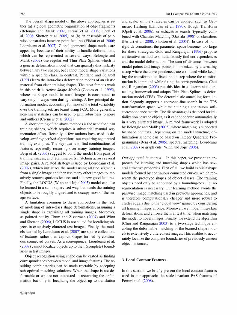
Fig. 10 Learned shape models for ETHZ Shape Classes (three out oftotal five per class). Top three rows: models learnt using the full methodpresented in Sect. 4. Last row: models learnt using the same trainingimages used in row 3, but skipping the procedure for assembling theinitial shape (Sect. 4.2; done only for ETHZ shape classes)
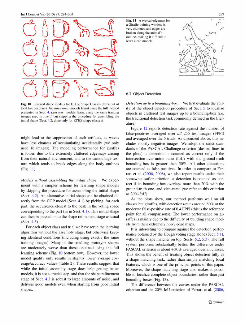
might lead to the suppression of such artifacts, as waveshave less chances of accumulating accidentally (we onlyused 16 images). The modeling performance for giraffesis lower, due to the extremely cluttered edgemaps arisingfrom their natural environment, and to the camouflage tex-ture which tends to break edges along the body outlines(Fig. 11).
Models without assembling the initial shape. We exper-iment with a simpler scheme for learning shape modelsby skipping the procedure for assembling the initial shape(Sect. 4.2). An alternative initial shape can be obtained di-rectly from the COP model (Sect. 4.1) by picking, for eachpart, the occurrence closest to the peak in the voting spacecorresponding to the part (as in Sect. 4.1). This initial shapecan then be passed on to the shape refinement stage as usual(Sect. 4.3).
For each object class and trial we have rerun the learningalgorithm without the assembly stage, but otherwise keep-ing identical conditions (including using exactly the sametraining images). Many of the resulting prototype shapesare moderately worse than those obtained using the fulllearning scheme (Fig. 10 bottom row). However, the lowermodel quality only results in slightly lower average cov-erage/accuracy values (Table 2). These results suggest thatwhile the initial assembly stage does help getting bettermodels, it is not a crucial step, and that the shape refinementstage of Sect. 4.3 is robust to large amounts of noise, anddelivers good models even when starting from poor initialshapes.
Fig. 11 A typical edgemap fora Giraffe training window isvery cluttered and edges arebroken along the animal’soutline, making it difficult tolearn clean models
6.3 Object Detection
Detection up to a bounding-box. We first evaluate the abil-ity of the object detection procedure of Sect. 5 to localizeobjects in cluttered test images up to a bounding-box (i.e.the traditional detection task commonly defined in the liter-ature).
Figure 12 reports detection-rate against the number offalse-positives averaged over all 255 test images (FPPI)and averaged over the 5 trials. As discussed above, this in-cludes mostly negative images. We adopt the strict stan-dards of the PASCAL Challenge criterion (dashed lines inthe plots): a detection is counted as correct only if theintersection-over-union ratio (IoU) with the ground-truthbounding-box is greater than 50%. All other detectionsare counted as false-positives. In order to compare to Fer-rari et al. (2006, 2008), we also report results under theirsomewhat softer criterion: a detection is counted as cor-rect if its bounding-box overlaps more than 20% with theground-truth one, and vice-versa (we refer to this criterionas 20%-IoU).
As the plots show, our method performs well on allclasses but giraffes, with detections-rates around 80% at themoderate false-positive rate of 0.4 FPPI (this is the referencepoint for all comparisons). The lower performance on gi-raffes is mainly due to the difficulty of building shape mod-els from their extremely noisy edge maps.
It is interesting to compare against the detection perfor-mance obtained by the Hough voting stage alone (Sect. 5.1),without the shape matcher on top (Sects. 5.2, 5.3). The fullsystem performs substantially better: the difference underPASCAL criterion is about +30% averaged over all classes.This shows the benefit of treating object detection fully asa shape matching task, rather than simply matching localfeatures, which is one of the principal points of this paper.Moreover, the shape matching stage also makes it possi-ble to localize complete object boundaries, rather than justbounding-boxes (Fig. 13).
The difference between the curves under the PASCALcriterion and the 20%-IoU criterion of Ferrari et al. (2006,

298 Int J Comput Vis (2010) 87: 284–303
Fig. 12 (Color online) Object detection performance (models learntfrom real images). Each plot shows five curves: the full system evalu-ated under the PASCAL criterion for a correct detection (dashed, thick,red), the full system under the 20%-IoU criterion (solid, thick, red), the
Hough voting stage alone under PASCAL (dashed, thin, blue), (Ferrariet al. 2008) under 20%-IoU (solid, thin, green) and under PASCAL(dashed, thin, green). The curve for the full system under PASCAL inthe apple-logo plot is identical to the curve for 20%-IoU
2008) is small for apple-logos, bottles, mugs and swans(0%, −1.6%, −3.6%, −4.9%), indicating that most de-tections have accurate bounding-boxes. For horses and gi-raffes the decrease is more significant (−18.1%,−14.1%),because the legs of the animals are harder to detect andcause the bounding-box to shift along the body. On averageover all classes, our method achieves 78.1% detection-rateat 0.4 FPPI under 20%-IoU and 71.1% under PASCAL. Thecorresponding standard-deviation over trials, averaged overclasses, is 8.1% under 20%-IoU and 8.0% under PASCAL(this variation is due to different trials having different train-ing and test sets).
For reference, the plots also show the performance of Fer-rari et al. (2008) on the same datasets, using the same num-ber of training and test images. An exact comparison is notpossible, as Ferrari et al. (2008) reports result based on onlyone training/testing split, whereas we average over 5 randomsplits. Under the rather permissive 20%-IoU criterion, Fer-rari et al. (2008) performs a little better than our method onaverage over all classes. Under the strict PASCAL criterioninstead, our method performs substantially better than Fer-rari et al. (2008) on two classes (apple-logos, swans), mod-erately worse on two (bottles, horses), and about the sameon two (mugs, giraffes), thanks to the higher accuracy of
the detected bounding-boxes. Averaged over all classes, un-der PASCAL our method reaches 71.1% detection-rate at0.4 FPPI, comparing well against the 68.5% of Ferrari et al.(2008). Note how our results are achieved without the bene-ficial discriminative learning of Ferrari et al. (2008), wherea SVM learns which PAS types at which relative locationwithin the training bounding-box best discriminate betweeninstances of the class and background image windows. Ourmethod instead trains only from positive examples.
For clarity and reference for comparison by futureworks, we summarize here our results on the ETHZ ShapeClasses alone (without INRIA horses). Under PASCAL, av-eraged over all 5 trials and 5 classes, our method achieves72.0%/67.2% detection-rate at 0.4/0.3 FPPI respectively.Under 20%-IoU, it achieves 76.8%/71.5% detection-rate at0.4/0.3 FPPI.
After our results were first published (Ferrari et al. 2007),Fritz and Schiele (2008) presented an approach based ontopic models and a dense gradient histogram representationof image windows (no explicit shapes). They report resultson the ETHZ Shape Classes dataset (i.e. no horses), usingthe same protocol (5 random trials). Their method achieves84.8% averaged over classes, improving over our 76.8%(both at 0.4 FPPI and under 20%-IoU).

Int J Comput Vis (2010) 87: 284–303 299
Fig. 13 Example detections (models learnt from images). Notice thelarge scale variations (especially in apple-logos, swans), the intra-category shape variability (especially in swans, giraffes), and the ex-tensive clutter (especially in giraffes, mugs). The method works forphotographs as well as paintings (first swan, last bottle). Two bottle
cases show also false-positives. In the first two horse images, the hor-izontal line below the horses’ legs is part of the model and representsthe ground. Interestingly, the ground line systematically reoccurs overthe training images for that model and gets learned along with the horse
Beyond the above quantitative evaluation, the methodpresented in this paper offers two important advantages overboth Ferrari et al. (2008) and Fritz and Schiele (2008). It lo-
calizes object boundaries, rather than just bounding-boxes,and can also detect objects starting from a single hand-drawing as a model (see below).

300 Int J Comput Vis (2010) 87: 284–303
Table 3 Accuracy of localizedobject boundaries at test time.Each entry is the averagecoverage/precision over trialsand correct detections at0.4 FPPI
apple bottle giraffe mug swan
Full system 91.6 / 93.9 83.6 / 84.5 68.5 / 77.3 84.4 / 77.6 77.7 / 77.2
No learned deform 91.3 / 93.6 82.7 / 84.2 68.4 / 77.7 83.2 / 75.7 78.4 / 77.0
Ground-truth BB 42.5 / 40.8 71.2 / 67.7 26.7 / 29.8 55.1 / 62.3 36.8 / 39.3
Fig. 14 (Left) typical improvement brought by constrained shapematching over simply using the TPS deformation model. As the im-provement is often a refinement of a local portion of the shape (theswan’s tail in this case), the numerical differences in the evaluation
measures is only modest (in this case less than 1%). (Right) an infre-quent case, where constrained shape matching fixes the entirely wrongsolution delivered by standard matching. The numerical difference insuch cases is noticeable (about 6%)
Localizing object boundaries. The most interesting featureof our approach is the ability to localize object boundariesin novel test images. This is shown by several examples inFig. 13, where the method succeeds in spite of extensiveclutter, a large range of scales, and intra-class variability(typical failure cases are discussed in Fig. 16). In the fol-lowing we quantify how accurately the output shapes matchthe true object boundaries. We use the coverage and preci-sion measures defined above. In the present context, cover-age is the percentage of ground-truth boundary points recov-ered by the method and precision is the percentage of out-put points that lie on the ground-truth boundaries. All shapemodels used in these experiments have been learned fromreal images, as discussed before. Several models for eachobject class are shown in Figs. 10 and 15.
Table 3 shows coverage and precision averaged over tri-als and correct detections at 0.4 FPPI. Coverage rangesin 78–92% for all classes but giraffes, demonstrating thatmost of the true boundaries have been successfully detected.Moreover, precision values are similar, indicating that themethod returns only a small proportion of points outside thetrue boundaries. Performance is lower for giraffes, due tothe more noisy models and difficult edgemaps derived fromthe test images.
Although it uses the same evaluation metric, the exper-iment carried out at training time in Sect. 6.2 differs sub-stantially from the present one, because at testing time thesystem is not given ground-truth bounding-boxes. In spiteof the important additional challenge of having to deter-mine the object’s location and scale in the image, the cover-age/precision scores in Table 3 are only moderately lowerthan those achieved during training (Table 3; the average
difference in coverage and precision is 7.1% and 2.1% re-spectively). This demonstrates that our detection approachis highly robust to clutter.
As a baseline, Table 3 also reports coverage/precisionresults when using the ground-truth bounding-boxes asshapes. The purpose of this experiment is to compare theaccuracy of our method to the maximal accuracy that can beachieved when localizing objects up to a bounding-box. Asthe table clearly shows, the shapes returned by our methodare substantially more accurate than the best bounding-box,thereby proving one of the principal points of this paper.While the average difference is about 35%, it is interestingto observe how the difference is greater for less rectangularobjects (swans, giraffes, apple-logos) than for bottles andmugs. Notice also how our method is much more accuratethan the ground-truth bounding-box even for giraffes, theclass where it performs the worst.
Finally, we investigate the impact of the constrainedshape matching technique proposed in Sect. 5.3, by re-running the experiment without it, simply relying on thedeformation model implicit in the thin-plate spline formu-lation (Table 3, second row). The coverage/precision valuesare very similar to those obtained through constrained shapematching. The reason is that most cases are either alreadysolved accurately without learned deformation models, orthey do not improve when using them because the low ac-curacy is due to particularly bad edgemaps. In practice, thedifference made by constrained shape matching is visiblein about one case every six, and it is localized to a rela-tively small region of the shape (Fig. 14). The combinationof these two factors explains why constrained shape match-

Int J Comput Vis (2010) 87: 284–303 301
ing appears to make little quantitative difference, althoughin many cases the localized boundaries improve visibly.
Detection from hand-drawn models. A useful character-istic of the proposed approach is that, unlike most exist-ing object detection methods, it can take either a hand-drawing as a model, or learn it from real images. Whengiven a hand-drawing as a model, our approach does notperform the learning stage, and naturally falls back to thefunctionality of pure shape matchers which takes a cleanshape as input (e.g. the recent works (Ferrari et al. 2006;Schwartz and Felzenszwalb 2007), which support matchingto cluttered test images). In this case, the modeling stagesimply decomposes the hand-drawing into PAS. Object de-tection then uses these PAS for the Hough voting stage, andthe hand-drawing itself for the shape matching stage. Asno deformation model can be learnt from a single example,our method naturally switches to the standard deformationmodel implicit in the Thin-Plane Spline formulation.
Figure 17 compares our method to Ferrari et al. (2006)using their exact setup, i.e. with a single hand-drawing perclass as model and all 255 images of the ETHZ shapeclasses as test set. Therefore, the test set for each classcontains mostly images not containing any instance of theclass, which supports the proper estimation of FPPI. Ourmethod performs better than Ferrari et al. (2006) on all5 classes, especially in the low FPPI range, and substan-tially outperforms the oriented chamfer matching baseline(details in Ferrari et al. 2006). Averaged over classes, ourmethod achieves 85.3%/82.4% detection-rate at 0.4/0.3FPPI respectively, compared to 81.5%/70.5% of Ferrari etal. (2006) (all results under 20%-IoU). As one reason for thisimprovement, our method is more robust because it does notneed the test image to contain long chains of contour seg-ments around the object.
After our results were first published (Ferrari et al. 2007),two works reported even better performance. Ravishankar et
al. (2008) achieve 95.2% at 0.4 FPPI. Zhu et al. (2008) re-ports 0.21 FPPI at 85.3% detection-rate (ours). Note this isthe opposite of the usual way, reporting detection-rate at areference FPPI (Ferrari et al. 2006, 2007, 2008; Fritz andSchiele 2008; Ravishankar et al. 2008). All results are under20%-IoU and averaged over classes. As part of the reasonfor the high performance, Ravishankar et al. (2008) proposea sophisticated scoring method which allows to reliably re-ject false-positives, while the method of Zhu et al. (2008) re-lies on their algorithm (Zhu et al. 2007) to find long salientcontours, effectively removing many clutter edgels beforethe object detector runs. An interesting avenue for furtherresearch is incorporating these successful elements in ourframework.
Beside this quantitative evaluation, the main advantageof our approach over Ferrari et al. (2006), Ravishankar et al.(2008) and Zhu et al. (2008) is that it can also train from realimages (which is the main topic of this paper). Moreover,compared to Ferrari et al. (2006), it supports branching andself-intersecting input shapes.
Interestingly, in our system hand-drawings lead to mod-erately better detection results than when learning modelsfrom images. This is less surprising when considering thathand-drawings are essentially the prototype shapes the sys-tem tries to learn.
Fig. 15 Learned shape models for INRIA horses (three out of totalfive), using the method presented in Sect. 4
Fig. 16 Example failed detections (models learnt from images).(a) A typical case. A good match to the image edges is found, butat the wrong scale. Our system has no bias for any particular scale.(b) Another typical case. Failure is due to an extremely cluttered edge-map. The neck is correctly matched, and gives rise to a peak in the
Hough voting space (Sect. 5.1). However, the subsequent deformablematching stage (Sect. 5.2) is attracted by the high contrast waves inthe background. (c) An infrequent case. Failure is due to a poor shapemodel (right, this the worst of the 30 models we have learned)

302 Int J Comput Vis (2010) 87: 284–303
Fig. 17 (Color online) Object detection performance (hand-drawn models). To facilitate comparison, all curves have been computed using the20% -IoU criterion of Ferrari et al. (2006)
Fig. 18 Detection from hand-drawn models. Top: four of the five models from Ferrari et al. (2006). There is just one example per object class.Bottom: example detections delivered by our shape matching procedure, using these hand-drawings as models
7 Conclusions and Future Work
We have proposed an approach for learning class-specificexplicit shape models from images annotated by bounding-boxes, and localizing the boundaries of novel class instancesin the presence of extensive clutter, scale changes, and intra-class variability. In addition, the approach operates effec-tively also when given hand-drawings as models. The abilityto input both images and hand-drawings as training data is a
consequence of the basic design of our approach, which at-tempts to bridge the gap between shape matching and objectclass detection.
The presented approach can be extended in several ways.First, the training stage models only positive examples. Thiscould be extended by learning a classifier to distinguish be-tween positive and negative examples, which might reducefalse positives. One possibility could be to train both ourshape models and the discriminative models of Ferrari et al.

Int J Comput Vis (2010) 87: 284–303 303
(2008). At detection time, we could then use the bounding-box delivered by Ferrari et al. (2008) to initialize shapematching based on our models. Moreover, the discrimina-tive power of the representation could be improved by usingappearance features in addition to image contours. Finally,in this paper we have assumed that all observed differencesin the shape of the training examples originate from intra-class variation, and not from viewpoint changes. It would beinteresting to add a stage to automatically group objects byviewpoint, and learn separate shape models.
References
Basri, R., Costa, L., Geiger, D., & Jacobs, D. (1998). Determining thesimilarity of deformable shapes. Vision Research, 38, 2365–2385.
Belongie, S., & Malik, J. (2002). Shape matching and object recogni-tion using shape contexts. Pattern Analysis and Machine Intelli-gence, 24(4), 509–522.
Berg, A., Berg, T., & Malik, J. (2005). Shape matching and objectrecognition using low distortion correspondence, CVPR.
Borenstein, E., & Ullman, S. (2002). Class-specific, top-down segmen-tation, ECCV.
Chui, H., & Rangarajan, A. (2003). A new point matching algorithmfor non-rigid registration. CVIU, 89(2–3), 114–141.
Chum, O., & Zisserman, A. (2007). An exemplar model for learningobject classes, CVPR.
Cootes, T. (2000). An introduction to active shape models.Cootes, T., Taylor, C., Cooper, D., & Graham, J. (1995). Active shape
models: Their training and application. CVIU, 61(1), 38–59.Cremers, D., Kohlberger, T., & Schnorr, C. (2002). Nonlinear shape
statistics in Mumford-Shah based segmentation, ECCV.Dalal, N., & Triggs, B. (2005). Histograms of oriented gradients for
human detection, CVPR.Elidan, G., Heitz, G., & Koller, D. (2006). Learning object shape:
From drawings to images, CVPR.Felzenswalb, P. (2005). Representation and detection of deformable
shapes. Pattern Analysis and Machine Intelligence, 27(2), 208–220.
Fergus, R., Perona, P., & Zisserman, A. (2003). Object class recogni-tion by unsupervised scale-invariant learning, CVPR.
Ferrari, V., Tuytelaars, T., & van Gool, L. (2004). Simultaneous objectrecognition and segmentation by image exploration, ECCV.
Ferrari, V., Tuytelaars, T., & Van Gool, L. (2006). Object detection withcontour segment networks, ECCV.
Ferrari, V., Jurie, F., & Schmid, C. (2007). Accurate object detectionwith deformable shape models learnt from images, CVPR.
Ferrari, V., Fevrier, L., Jurie, F., & Schmid, C. (2008). Groups of adja-cent contour segments for object detection. Pattern Analysis andMachine Intelligence, 30(1), 36–51.
Fritz, M., & Schiele, B. (2006). Towards unsupervised discovery ofvisual categories, DAGM.
Fritz, M., & Schiele, B. (2008). Decomposition, discovery and detec-tion of visual categories using topic models, CVPR.
Gavrila, D. (1998). Multi-feature hierarchical template matching usingdistance transforms, ICPR.
Gdalyahu, Y., & Weinshall, D. (1999). Flexible syntactic matching ofcurves and its application to automatic hierarchical classificationof silhouettes. Pattern Analysis and Machine Intelligence, 21(12),1312–1328.
Gold, S., & Rangarajan, A. (1996). Graduated assignment algorithmfor graph matching. Pattern Analysis and Machine Intelligence,18(4), 377–388.
Hill, A., & Taylor, C. (1996). A method of non-rigid correspondencefor automatic landmark identification, BMVC.
Jurie, F., & Schmid, C. (2004). Scale-invariant shape features forrecognition of object categories, CVPR.
Lamdan, Y., Schwartz, J., & Wolfson, H. (1990). Affine invariantmodel-based object recognition. IEEE Transactions on Roboticsand Automation, 6(5), 578–589.
Leibe, B., & Schiele, B. (2004). Scale-invariant object categorizationusing a scale-adaptive mean-shift search, DAGM.
Leordeanu, M., Hebert, M., & Sukthankar, R. (2007). Beyond localappearance: Category recognition from pairwise interactions ofsimple features, CVPR.
Martin, D., Fowlkes, C., & Malik, J. (2004). Learning to detect naturalimage boundaries using local brightness, color, and texture cues.Pattern Analysis and Machine Intelligence, 26(5), 530–549.
Mokhtarian, F., & Mackworth, A. (1986). Scale-based description andrecognition of planar curves and two-dimensional shapes. PatternAnalysis and Machine Intelligence, 8(1), 34–43.
Opelt, A., Pinz, A., & Zisserman, A. (2006). A boundary-fragment-model for object detection, ECCV.
Pentland, A., & Sclaroff, S. (1991). Closed-form solutions for physi-cally based shape modeling and recognition. Pattern Analysis andMachine Intelligence, 13(7), 715–729.
Quack, T., Ferrari, V., Leibe, B., & Van Gool, L. (2007). Efficient min-ing of frequent and distinctive feature configurations, ICCV.
Ramanan, D. (2006). Learning to parse images of articulated bodies,NIPS.
Ravishankar, S., Jain, A., & Mittal, A. (2008). Multi-stage contourbased detection of deformable objects, ECCV.
Schwartz, J., & Felzenszwalb, P. (2007). Hierarchical matching of de-formable shapes, CVPR.
Sharvit, D., Chan, J., Tek, H., & Kimia, B. (1998). Symmetry-basedindexing of image databases. IEEE workshop on content-basedaccess of image and video libraries.
Shotton, J., Blake, A., & Cipolla, R. (2005). Contour-based learningfor object detection, ICCV.
Sebastian, T., Klein, P., & Kimia, B. (2004). Recognition of shapes byediting their shock graphs. Pattern Analysis and Machine Intelli-gence, 26(5), 550–571.
Torralba, A., Murphy, K., & Freeman, W. (2004). Sharing features:Efficient boosting procedures for multiclass object detection,CVPR.
Winn, J., & Jojic, N. (2005). LOCUS: Learning object classes withunsupervised segmentation, ICCV.
Winn, J., & Shotton, J. (2006). The layout consistent random field forrecognizing and segmenting partially occluded objects, CVPR.
Zhu, Q., Song, G., & Shi, J. (2007). Untangling cycles for contourgrouping, ICCV.
Zhu, Q., Wang, L., Wu, Y., & Shi, J. (2008). Contour context selec-tion for object detection: A set-to-set contour matching approach,ECCV.