From Certainty Factors to Belief Networks

David E. Heckerman∗

<dheck@sumex-aim.stanford.edu>Edward H. Shortliffe

<ehs@sumex-aim.stanford.edu>

Section on Medical InformaticsStanford University School of Medicine

MSOB X-215, 300 Pasteur DriveStanford, CA 94305-5479

To appear in Artificial Intelligence in Medicine, 1992.

∗Current address: Departments of Computer Science and Pathology, University of Southern California,HMR 204, 2025 Zonal Avenue, Los Angeles, CA 90033.

1

Abstract

The certainty-factor (CF) model is a commonly used method for managing uncertaintyin rule-based systems. We review the history and mechanics of the CF model, anddelineate precisely its theoretical and practical limitations. In addition, we examinethe belief network, a representation that is similar to the CF model but that is groundedfirmly in probability theory. We show that the belief-network representation overcomesmany of the limitations of the CF model, and provides a promising approach to thepractical construction of expert systems.

Keywords: certainty factor, probability, belief network, uncertain reasoning, expertsystems

2

1 IntroductionIn this issue of the journal, Dan and Dudeck provide a critique of the certainty-factor (CF)model, a method for managing uncertainty in rule-based systems. Shortliffe and Buchanandeveloped the CF model in the mid-1970s for MYCIN, an early expert system for the diagno-sis and treatment of meningitis and bacteremia [38, 37]. Since then, the CF model has beenwidely adopted in a variety of expert-system shells and in individual rule-based systems thathave had to reason under uncertainty. Although we concur with many of the observationsin the article by Dan and Dudeck, we believe that the reasons for the development of theCF model must be placed in historical context, and that it is important to note that the AIresearch community has largely abandoned the use of CFs. In our laboratory, where the CFmodel was originally developed, we have not used CFs in our systems for over a decade. Weaccordingly welcome the opportunity to review the CF model, the reasons for its creation,and recent developments and analyses that have allowed us to turn in new directions forapproaches to uncertainty management.

When the model was created, many artificial-intelligence (AI) researchers expressed con-cern about using Bayesian (or subjective) probability to represent uncertainty. Of theseresearchers, most were concerned about the practical limitations of using probability theory.In particular, builders of probabilistic diagnostic systems for medicine and other domainshad largely been using the simple-Bayes model. This model included the assumptions that(1) faults or hypotheses were mutually exclusive and exhaustive, and (2) pieces of evidencewere conditionally independent, given each fault or hypothesis (see Section 3). The assump-tions were useful, because their adoption had made the construction of diagnostic systemspractical. Unfortunately, the assumptions were often inaccurate in practice.

The reasons for creating the CF model were described in detailed in the original paperby Shortliffe and Buchanan [38]. The rule-based approach they were developing required amodular approach to uncertainty management, and efforts to use a Bayesian model in thiscontext had been fraught with difficulties. Not only were they concerned about the assump-tions used in the simple-Bayes model, but they wanted to avoid the cognitive complexitythat followed from dealing with large numbers of conditional and prior probabilities. Theyalso found that it was difficult to assess subjective probabilities from experts in a way thatwas internally consistent. Furthermore, initial interactions with their experts led them to be-lieve that the numbers being assigned by the physicians with whom they were working weredifferent in character from probabilities. Thus, the CF model was created for the domain ofMYCIN as a practical approach to uncertainty management in rule-based systems. Indeed,in blinded evaluations of MYCIN, the CF model provided recommendations for treatmentthat were judged to be equivalent to, or better than, therapy plans provided by infectiousdisease experts for the same cases [47, 48].

Despite the success of the CF model for MYCIN, its developers warned researchers andknowledge engineers that the model had been designed for a domain with unusual charac-teristics, and that the model’s performance might be sensitive to the domain of application.Clancey and Cooper’s sensitivity analysis of the CF model [4, Chapter 10] demonstrated thatMYCIN’s therapy recommendations were remarkably insensitive to perturbations in the CF

3

values assigned to rules in the system. MYCIN’s diagnostic assessments, however, showedmore rapid deterioration as CF values were altered. Since MYCIN was primarily a therapyadvice system, and since antibiotic therapies often cover for many pathogens, variations indiagnostic hypotheses often had minimal effect on the therapy that was recommended; incertain cases where perturbations in CFs led to an incorrect diagnosis, the treatments rec-ommended by the model were still appropriate. This observation suggests strongly that theCF model may be inadequate for diagnostic systems or in domains where appropriate recom-mendations of treatment are more sensitive to accurate diagnosis. Unfortunately, this pointhas been missed by many investigators who have built expert systems using CFs or haveincorporated the CF model as the uncertainty management scheme for some expert-systemshells.

In this article, we reexamine the CF model, illustrating both its theoretical and practicallimitations. In agreement with Shortliffe and Buchanan’s original view of the model, we seethat CFs do not correspond to probabilities. We find, however, that CFs can be interpreted asmeasures of change in belief within the theory of probability. If one interprets the CF modelin this way, we show that, in many circumstances, the model implicitly imposes assumptionsthat are stronger than those of the simple-Bayes model. We trace the flaws in the model to itsimposition of the same sort of modularity on uncertain rules that we accept for logical rules,and we show that uncertain reasoning is inherently less modular than is logical reasoning.Also, we argue that the assessment of CFs is often more difficult and less reliable than is theassessment of conditional probabilities. Most important, we describe an alternative to theCF model for managing uncertainty in expert systems. In particular, we discuss the beliefnetwork, a graphical representation of beliefs in the probabilistic framework. We see thatthis representation overcomes many of the difficulties associated with both the simple-Bayesand CF models. In closing, we point to recent research that shows that diagnostic systemsconstructed using belief networks can be practically applied in real-world clinical settings.

2 The Mechanics of the ModelTo understand how the CF model works, let us consider a simple example adapted from Kimand Pearl [25]:

Mr. Holmes receives a telephone call from Eric, his neighbor. Eric notifiesMr. Holmes that he has heard a burglar alarm sound from the direction of Mr.Holmes’ home. About a minute later, Mr. Holmes receives a telephone call fromCynthia, his other neighbor, who gives him the same news.

A miniature rule-based system for Mr. Holmes’ situation contains the following rules:

R1: if ERIC’S CALL then ALARM, CF1 = 0.8

R2: if CYNTHIA’S CALL then ALARM, CF2 = 0.9

R3: if ALARM then BURGLARY, CF3 = 0.7

4

ALARM

ERIC�S CALL

CYNTHIA�S CALL

BURGLARY

0.8

0.9

0.7

Figure 1: An inference network for Mr. Holmes’ situation.Each arc represents a rule. For example, the arc from ALARM to BURGLARY represents the ruleR3 (“if ALARM then BURGLARY”). The number above the arc is the CF for the rule. The CF of0.7 indicates that burglar alarms can go off for reasons other than burglaries. The CFs of 0.8 and0.9 indicate that Mr. Holmes finds Cynthia to be slightly more reliable than Eric. (Figure takenfrom D. Heckerman, The Certainty-Factor Model, S. Shapiro, editor, Encyclopedia of ArtificialIntelligence, Second Edition. Wiley, New York.)

In general, rule-based systems contain rules of the form “if e then h,” where e denotes apiece of evidence for hypothesis h. Using the CF model, an expert represents his uncertaintyin a rule by attaching a single CF to each rule.

Shortliffe and Buchanan intended a CF to represent a person’s (usually, the expert’s)change in belief in the hypothesis given the evidence. In particular, a CF between 0 and1 means that the person’s belief in h given e increases, whereas a CF between -1 and 0means that the person’s belief decreases. The developers of the model did not intend a CFto represent a person’s absolute degree of belief in h given e, as does a probability [38]. Wereturn to this point in Section 4.3.

Several implementations of rule-based representation of knowledge display a rule base ingraphical form as an inference network. Figure 1 illustrates the inference network for Mr.Holmes’ situation. Each arc in an inference network represents a rule; the number above thearc is the CF for the rule.

Using the CF model, we can compute the change in belief in any hypothesis in thenetwork, given the observed evidence. We do so by applying simple combination functionsto the CFs that lie between the evidence and the hypothesis in question. For example, inMr. Holmes’ situation, we are interested in computing the change in belief of BURGLARY,given that Mr. Holmes received both ERIC’S CALL and CYNTHIA’S CALL. We combine theCFs in two steps. First, we combine CF1 and CF2, the CFs for R1 and R2, to give the CFfor the new composite rule R4:

R4: if ERIC’S CALL and CYNTHIA’S CALL then ALARM, CF4

We combine CF1 and CF2 using the function

CF4 =

CF1 + CF2 − CF1CF2 CF1, CF2 ≥ 0

CF1 + CF2 + CF1CF2 CF1, CF2 < 0CF1+CF2

1−min(|CF1|,|CF2|) otherwise

(1)

5

For CF1 = 0.8 and CF2 = 0.9, we have

CF4 = 0.8 + 0.9− (0.8)(0.9) = 0.98

Equation 1 may be called the parallel-combination function.The earliest version of the CF model employed a parallel-combination function slightly

different from Equation 1. There, positive CFs—called MBs—were combined as in Equa-tion 1. Also, negative CFs—called MDs—were combined as in Equation 1. The final CF forthe hypothesis, however, was given as the difference between MB and MD. This combinationfunction has the following undesirable property. Let us suppose we have many strong piecesof evidence for a hypothesis. In particular, suppose that the combined certainty factor forthe hypothesis has asymptotically approached 1. In addition, suppose that we have oneweak piece of evidence against the same hypothesis, with a CF of -0.5. Using the originalcombination function, the net CF for the combined evidence would be approximately 0.5,which represents only weak evidence for the hypothesis. Shortliffe and Buchanan foundunappealing this ability of a single, weak piece of negative evidence to overwhelm manypieces of positive evidence. Consequently, they and van Melle modified the function to thatdescribed by Equation 1 [44]. In this issue, Dan and Dudek argue that the original combi-nation function is satisfactory. We find the argument made here more compelling then theirargument.

Second, we combine CF3 and CF4, to give the CF for the new composite rule R5:

R5: if ERIC’S CALL and CYNTHIA’S CALL then BURGLARY, CF5

The combination function is

CF5 =

CF3CF4 CF3 > 0

0 CF3 ≤ 0(2)

In Mr. Holmes’ case, we have

CF5 = (0.98)(0.7) = 0.69

Equation 2 may be called the serial-combination function. The CF model prescribes thisfunction to combine two rules where the hypothesis in the first rule is the evidence in thesecond rule (i.e., when the rules “chain” together).

If all evidence and hypotheses in a rule base are simple propositions, we need to useonly the serial and parallel combination rules to combine CFs. The CF model, however,also incorporated combination functions to accommodate rules that contain conjunctionsand disjunctions of evidence. For example, suppose we have the following rule in an expertsystem for diagnosing chest pain:

R6: if CHEST PAIN andSHORTNESS OF BREATH

then HEART ATTACK, CF6 = 0.9

6

Further, suppose that we have rules that reflect indirect evidence for chest pain and shortnessof breath:

R7: if PATIENT GRIMACES then CHEST PAIN, CF7 = 0.7

R8: if PATIENT CLUTCHES THROAT then SHORTNESS OF BREATH, CF8 = 0.9

We can combine CF6, CF7, and CF8 to yield the CF for the new composite rule R9:

R9: if PATIENT GRIMACES andPATIENT CLUTCHES THROAT

then HEART ATTACK, CF9

The combination function is

CF9 = CF6 min(CF7, CF8) = (0.9)(0.7) = 0.63 (3)

That is, we compute the serial combination of CF6 and the minimum of CF7 and CF8. Weuse the minimum of CF7 and CF8, because R6 contains the conjunction of CHEST PAIN andSHORTNESS OF BREATH. In general, the CF model prescribes that we use the minimum ofCFs for evidence in a conjunction, and the maximum of CFs for evidence in a disjunction.

There are many variations among the implementations of the CF model. For example,the original CF model used in MYCIN treats CFs less than 0.2 as though they were 0 inserial combination, to avoid the generation of unnecessary questions to the the user under itsgoal-directed reasoning scheme. For the sake of brevity, we will not describe other variations,but they are thoroughly outlined in [4].

3 The Simple-Bayes and CF ModelsThe simple-Bayes model is restrictive, in part, because it includes the assumption that piecesof evidence are conditionally independent, given each hypothesis. In general, propositionsa and b are independent, if a person’s probability (or belief) of a does not change once bbecomes known. Propositions a and b are conditionally independent, given proposition c, ifa and b are independent when a person assumes or knows that c is true. Thus, in using thesimple-Bayes model, we assume that if we know which hypothesis is true, then observingone or more pieces of evidence does not change our probability that other pieces of evidenceare true.

In the simple case of Mr. Holmes, the CF model is an improvement over the simple-Bayesmodel. In particular, ERIC’S CALL and CYNTHIA’S CALL are not conditionally independent,given BURGLARY, because even if Mr. Holmes knows that a burglary has occurred, receivingEric’s call increases Mr. Holmes belief that Cynthia will call. The lack of conditionalindependence is due to the triggering of calls by the sound of the alarm, and not by theburglary. In this example, the CF model represents accurately this lack of independencethrough the presence of ALARM in the inference network.

Unfortunately, the CF model cannot represent most real-world problems in a way that isboth accurate and efficient. This limitation may not be serious in domains such as MYCIN’s,

7

but it does call into question the use of the CF model as a general method for managinguncertainty. In the next section, we shall see that the assumptions of conditional indepen-dence associated with the parallel-combination function are stronger (i.e., are less likely tobe accurate) than are those associated with the simple-Bayes model.

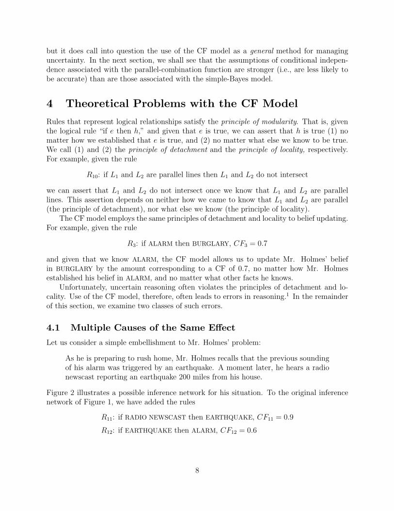
4 Theoretical Problems with the CF ModelRules that represent logical relationships satisfy the principle of modularity. That is, giventhe logical rule “if e then h,” and given that e is true, we can assert that h is true (1) nomatter how we established that e is true, and (2) no matter what else we know to be true.We call (1) and (2) the principle of detachment and the principle of locality, respectively.For example, given the rule

R10: if L1 and L2 are parallel lines then L1 and L2 do not intersect

we can assert that L1 and L2 do not intersect once we know that L1 and L2 are parallellines. This assertion depends on neither how we came to know that L1 and L2 are parallel(the principle of detachment), nor what else we know (the principle of locality).

The CF model employs the same principles of detachment and locality to belief updating.For example, given the rule

R3: if ALARM then BURGLARY, CF3 = 0.7

and given that we know ALARM, the CF model allows us to update Mr. Holmes’ beliefin BURGLARY by the amount corresponding to a CF of 0.7, no matter how Mr. Holmesestablished his belief in ALARM, and no matter what other facts he knows.

Unfortunately, uncertain reasoning often violates the principles of detachment and lo-cality. Use of the CF model, therefore, often leads to errors in reasoning.1 In the remainderof this section, we examine two classes of such errors.

4.1 Multiple Causes of the Same EffectLet us consider a simple embellishment to Mr. Holmes’ problem:

As he is preparing to rush home, Mr. Holmes recalls that the previous soundingof his alarm was triggered by an earthquake. A moment later, he hears a radionewscast reporting an earthquake 200 miles from his house.

Figure 2 illustrates a possible inference network for his situation. To the original inferencenetwork of Figure 1, we have added the rules

R11: if RADIO NEWSCAST then EARTHQUAKE, CF11 = 0.9

R12: if EARTHQUAKE then ALARM, CF12 = 0.6

8

ALARM

ERIC�S CALL

CYNTHIA�S CALL

BURGLARY

0.8

0.9

0.7

EARTHQUAKE

RADIO NEWSCAST

0.9

0.6

Figure 2: Another inference network for Mr. Holmes’ situation.In addition to the interactions in Figure 1, RADIO NEWSCAST increases the chance of EARTH-QUAKE, and EARTHQUAKE increases the chance of ALARM. (Figure taken from D. Heckerman,The Certainty-Factor Model, S. Shapiro, editor, Encyclopedia of Artificial Intelligence, Second Edi-tion. Wiley, New York.)

The inference network does not capture an important interaction among the propositions.In particular, the modular rule R3 (“if ALARM then BURGLARY”) gives us permission toincrease Mr. Holmes’ belief in BURGLARY, when his belief in ALARM increases, no matterhow Mr. Holmes increases his belief for ALARM. This modular license to update belief,however, is not consistent with common sense. When Mr. Holmes hears the radio newscast,he increases his belief that an earthquake has occurred. Therefore, he decreases his belief thatthere has been a burglary, because the occurrence of an earthquake would account for thealarm sound. Overall, Mr. Holmes’ belief in ALARM increases, but his belief in BURGLARYdecreases.

When the evidence for ALARM came from ERIC’S CALL and CYNTHIA’S CALL, we had noproblem propagating this increase in belief through R3 to BURGLARY. In contrast, when theevidence for ALARM came from EARTHQUAKE, we could not propagate this increase in beliefthrough R3. This difference illustrates a violation of the detachment principle in uncertainreasoning: the source of a belief update, in part, determines whether or not that updateshould be passed along to other propositions.

Pearl describes this phenomenon in detail [33, Chapter 1]. He divides uncertain rules intotwo types: diagnostic and predictive.2 In a diagnostic rule, we change the belief in a cause,given an effect. All the rules in the inference network of Figure 2, except R12, are of thisform. In a predictive rule, we change the belief in an effect, given a cause. R12 is an exampleof such an rule. Pearl describes the interactions between the two types of rules. He notesthat, if the belief in a proposition is increased by a diagnostic rule, then that increase can be

1Heckerman and Horvitz first noted the nonmodularity of uncertain reasoning, and the relationship ofsuch nonmodularity to the limitations of the CF model [18, 17]. Pearl first decomposed the principle ofmodularity into the principles of detachment and locality [33, Chapter 1].

2Henrion also makes this distinction [20].

9

passed through to another diagnostic rule—just what we expect for the chain of inferencesfrom ERIC’S CALL and CYNTHIA’S CALL to BURGLARY. On the other hand, if the belief in aproposition is increased by a predictive rule, then that belief should not be passed througha diagnostic rule. Moreover, when the belief in one cause of an observed effect increases,the beliefs in another cause should decrease—even when the two causes are not mutuallyexclusive. This interaction is just what we expect for the two causes of ALARM.

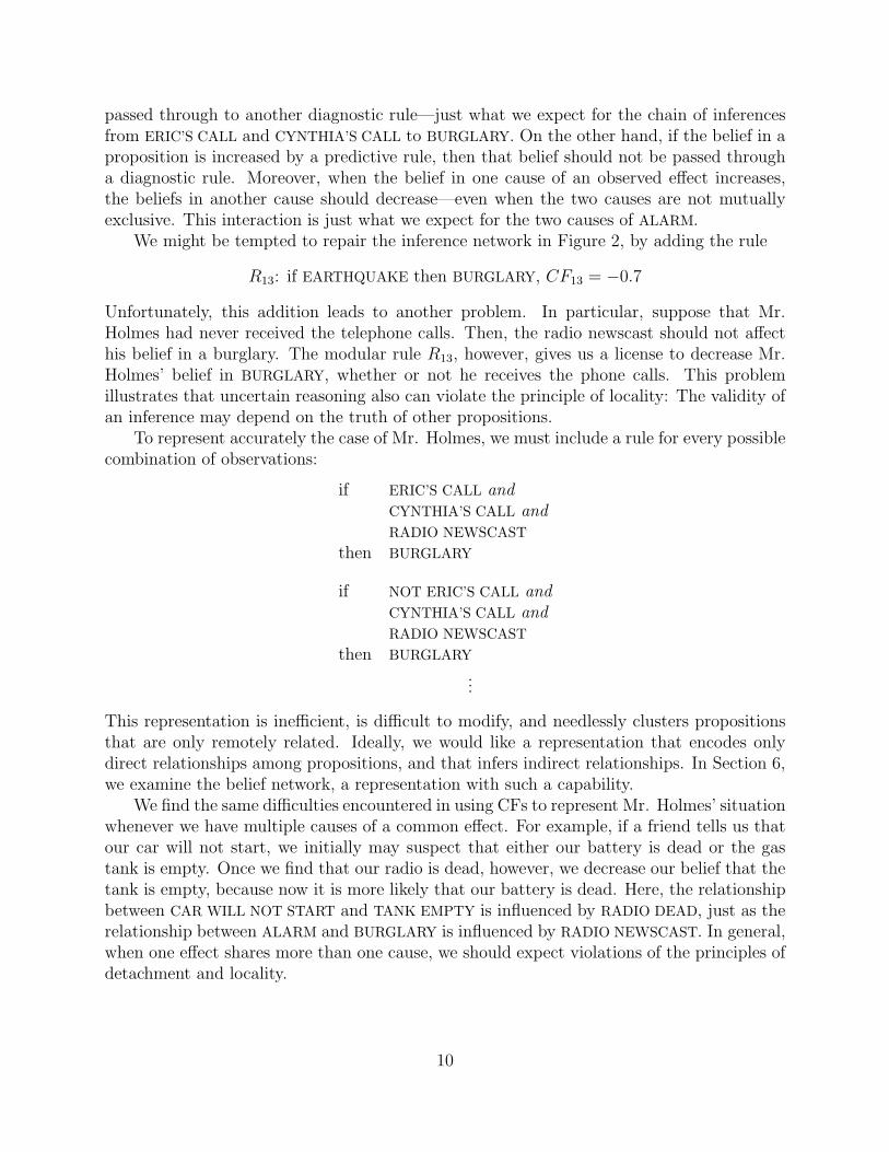
We might be tempted to repair the inference network in Figure 2, by adding the rule

R13: if EARTHQUAKE then BURGLARY, CF13 = −0.7

Unfortunately, this addition leads to another problem. In particular, suppose that Mr.Holmes had never received the telephone calls. Then, the radio newscast should not affecthis belief in a burglary. The modular rule R13, however, gives us a license to decrease Mr.Holmes’ belief in BURGLARY, whether or not he receives the phone calls. This problemillustrates that uncertain reasoning also can violate the principle of locality: The validity ofan inference may depend on the truth of other propositions.

To represent accurately the case of Mr. Holmes, we must include a rule for every possiblecombination of observations:

if ERIC’S CALL andCYNTHIA’S CALL andRADIO NEWSCAST

then BURGLARY

if NOT ERIC’S CALL andCYNTHIA’S CALL andRADIO NEWSCAST

then BURGLARY...

This representation is inefficient, is difficult to modify, and needlessly clusters propositionsthat are only remotely related. Ideally, we would like a representation that encodes onlydirect relationships among propositions, and that infers indirect relationships. In Section 6,we examine the belief network, a representation with such a capability.

We find the same difficulties encountered in using CFs to represent Mr. Holmes’ situationwhenever we have multiple causes of a common effect. For example, if a friend tells us thatour car will not start, we initially may suspect that either our battery is dead or the gastank is empty. Once we find that our radio is dead, however, we decrease our belief that thetank is empty, because now it is more likely that our battery is dead. Here, the relationshipbetween CAR WILL NOT START and TANK EMPTY is influenced by RADIO DEAD, just as therelationship between ALARM and BURGLARY is influenced by RADIO NEWSCAST. In general,when one effect shares more than one cause, we should expect violations of the principles ofdetachment and locality.

10

PHONE INTERVIEW

THOUSANDS DEAD

TV REPORT

RADIO REPORT

NEWSPAPER REPORT

Figure 3: An inference network for the Chernobyl disaster (adapted from [19]).When we combine CFs as modular belief updates, we overcount the chance of THOUSANDS DEAD.

4.2 Correlated EvidenceFigure 3 depicts an inference network for news reports about the Chernobyl disaster. Onhearing radio, television, and newspaper reports that thousands of people have died of ra-dioactive fallout, we increase substantially our belief that many people have died. When welearn that each of these reports originated from the same source, however, we decrease ourbelief. The CF model, however, treats both situations identically.

In this example, we see another violation of the principle of detachment in uncertain rea-soning: The sources of a set of belief updates can strongly influence how we combine thoseupdates. Because the CF model imposes the principle of detachment on the combination ofbelief updates, it overcounts evidence when the sources of that evidence are positively cor-related, and it undercounts evidence when the sources of evidence are negatively correlated.

4.3 Probabilistic Interpretations for Certainty FactorsAlthough the developers of MYCIN and derivative systems used the CF model and com-bining functions without explicitly depending upon a specific interpretation of the numbersthemselves, several researchers have assigned probabilistic interpretations to CFs. We canuse these interpretations to understand better the limitations of the CF model. In the origi-nal work describing the model, Shortliffe and Buchanan proposed the following approximateinterpretation:

CF (h→ e|ξ) =

p(h|e,ξ)−p(h|ξ)1−p(h|ξ) p(h|e, ξ) ≥ p(h|ξ)

p(h|e,ξ)−p(h|ξ)p(h|ξ) p(h|e, ξ) < p(h|ξ)

(4)

where CF (h→ e|ξ) is the CF for the rule “if e then h” given by an expert with backgroundknowledge ξ; p(h|ξ) is the expert’s probability (degree of belief) for h given ξ; and p(h|e, ξ) is

11

the expert’s probability for h given evidence e and ξ.3 Adams examined this interpretationin detail [1]. He proved that the the parallel combination function—with the exception ofthe combination of CFs of mixed sign—is consistent with the rules of probability, provided(1) evidence is marginally independent and (2) evidence is conditionally independent, givenh and NOT h.

Heckerman analyzed the model in a different way [12]. In particular, Heckerman showedthat Shortliffe and Buchanan’s probabilistic interpretation was inconsistent with the combi-nation functions that were used by MYCIN and its descendants. For example, he showedthat the probabilistic interpretation prescribes noncommutative parallel combination of ev-idence, even though the parallel combination function (Equation 1) is commutative.4 Giventhis inconsistency, Heckerman argued that either the probabilistic interpretation, the com-bination functions, or both components of the model must be reformulated. Heckerman,in contrast to Adams, argued that Shortliffe and Buchanan’s interpretation should be dis-carded, because he believed (as do Shortliffe and Buchanan) that the combination functionsare the cornerstone of the CF model; their proposed definitions (Equation 4) were simply anattempt to show how the numbers used by MYCIN might be interpreted.

Heckerman went on to show that we can interpret a certainty factor for hypothesis h,given evidence e, as a monotonic increasing function of the likelihood ratio

λ(h, e) =p(e|h, ξ)

p(e|NOT h, ξ)(5)

In particular, he showed that, if we make the identification

CF (h→ e|ξ) =

λ(h,e)−1λ(h,e) λ(h, e) ≥ 1

λ(h, e)− 1 λ(h, e) < 1(6)

then the parallel-combination function used by MYCIN (Equation 1) follows exactly from therules of probability. In addition, with the identification in Equation 6, the serial-combinationfunction (Equation 2) and the combination functions for disjunction and conjunction are closeapproximations to the rules of probability. Using Bayes’ theorem, we can write Equation 6as

CF (h→ e|ξ) =

p(h|e,ξ)−p(h|ξ)(1−p(h|ξ))p(h|e,ξ) p(h|e, ξ) ≥ p(h|ξ)

p(h|e,ξ)−p(h|ξ)p(h|ξ)(1−p(h|e,ξ)) p(h|e, ξ) < p(h|ξ)

(7)

This probabilistic interpretation for CFs differs from Shortliffe and Buchanan’s interpretationonly by an additional term in the denominator of each case. These extra terms make therelationship between the probabilities p(h|e, ξ) and p(h|ξ) symmetric. It is this symmetrythat makes this interpretation consistent with the combination functions.

3Shortliffe and Buchanan did not make the expert’s background knowledge ξ explicit. Nonetheless, inthe Bayesian interpretation of probability theory, a probability is always conditioned on the backgroundknowledge of the person who assesses that probability.

4In this issue, Dan and Dudeck dispute this demonstration. They argue that we must combine evidencebefore applying the interpretation. However, we do not see any reason why this or any other probabilisticinterpretation should be subjected to this limitation; a probabilistic interpretation should be limited only bythe rules of probability.

12

The original interpretation of CFs (Equation 4) reflects Shortliffe and Buchanan’s viewthat a CF represents a measure of change in belief (see the difference terms in the nu-merators). Nonetheless, in this interpretation, as p(h|ξ) approaches 0 with p(h|e, ξ) fixed,CF (h→ e|ξ) approaches p(h|e, ξ), a measure of absolute belief. The odd fact that a measureof change in belief can approach a measure of absolute belief led Shortliffe and Buchananto emphasize the approximate nature of their probabilistic interpretation. In fact, they hadspeculated that CFs may not admit any probabilistic interpretation. Heckerman’s interpre-tation, however, does not exhibit this unusual behavior. In particular, as p(h|ξ) approaches 0with p(h|e, ξ) fixed, CF (h→ e|ξ) approaches 1. This behavior is reasonable: If a hypothesisis extremely unlikely, we require a strong belief update to make that hypothesis at all likely.Thus, under the interpretation of the CF model as proposed by Heckerman, one can disputeprevious claims that the CF model is fundamentally different from the theory of probability.

Heckerman’s interpretation of CFs can help us to understand the limitations of themodel. In developing this interpretation, Heckerman showed that the parallel and serialcombination functions impose assumptions of conditional independence on the propositionsinvolved in the combinations. In particular, when we use the parallel-combination functionto combine CFs for the rules “if e1 then h” and “if e2 then h,” we assume implicitly thate1 and e2 are conditionally independent, given h and NOT h. Similarly, when we use theserial-combination function to combine CFs for the rules “if a then b” and “if b then c,” weassume implicitly that a and c are conditionally independent, given b and NOT b. Heckermanalso showed that the combination functions for disjunction and conjunction impose specificforms of conditional dependence on the propositions involved in the combinations [13].

Overall, Heckerman’s interpretation shows us that the independence assumptions im-posed by the CF model make the model inappropriate for many—if not most—real-worlddomains. Indeed, the assumptions of the parallel-combination function are stronger than arethose of the simple-Bayes model, the same model whose limitations motivated in part thedevelopment of the CF model. That is, when we use the simple-Bayes model, we assumethat evidence is conditionally independent given each hypothesis. When we use the parallel-combination function, however, we assume that evidence is conditionally independent giveneach hypothesis and the negation of each hypothesis. Unless the space of hypotheses con-sists of a single proposition and the negation of that proposition, the parallel-combinationassumptions are essentially impossible to satisfy, even when the simple-Bayes assumptionsare satisfied [23].

In closing this section, we comment on Dan and Dudek’s suggestion that CF (h →e|ξ) should be interpreted as a measure of the absolute belief in h, given e. In makingthis suggestion, they observe that most users of the model assess and use CFs as thoughthey were absolute measure of belief. Moreover, they argue that we should not seek aprobabilistic interpretation, because of the “inappropriate logical foundation” of probabilitytheory. The authors of this article disagree strongly with this view. First, we believe that—from a theoretical perspective—probability theory is the most appropriate representationof uncertain beliefs. The theory is self consistent and well developed, and allows for theunambiguous representation of independence assumptions. In addition, psychologists anddecision analysts have shown that the use of probability theory can help people avoid mistakes

13

in reasoning [6, 42, 40, 24]. We know of no other representation for uncertain beliefs thathave all of these benefits.

Second, if a CF (h → e|ξ) were to represent an expert’s absolute belief in h, given e,then the parallel combination of CFs for multiple pieces of evidence would overcount theexpert’s initial or prior belief in h. For example, let us suppose that e1 and e2 are twopieces of evidence for h. Because both CF (h → e1|ξ) and CF (h → e2|ξ) incorporate theexpert’s prior belief in h, we doublecount this prior belief when we combine the CFs using theparallel combination function. The observation that most people interpret CFs as measuresof absolute belief simply shows that most people are making this error; the observation isnot an argument for how we should interpret CFs.

4.4 A Fundamental DifferenceUnder Heckerman’s interpretation, we can identify precisely the problem with the CF repre-sentation of Mr. Holmes’ situation. There, we use serial combination to combine CFs for thesequence of propositions EARTHQUAKE, ALARM, and BURGLARY. In doing so, we make theinaccurate assumption (among others) that EARTHQUAKE and BURGLARY are conditionallyindependent, given ALARM. No matter how we manipulate the arcs in the inference networkof Figure 2, we generate inaccurate assumptions of conditional independence.

We can understand the problems with the CF model, however, at a more intuitive level.Logical relationships represent what we can observe directly. In contrast, uncertain relation-ships encode invisible influences: exceptions to that which is visible. For example, a burglarywill not always trigger an alarm, because there are hidden mechanisms that may inhibit thesounding of the alarm. We summarize these hidden mechanisms in a probability for ALARMgiven BURGLARY. In the process of summarization, we lose information. Therefore, whenwe try to combine uncertain information, unexpected (nonmodular) interactions may occur.We should not expect that the CF model—or any modular belief updating scheme—will beable to handle such subtle interactions. Pearl provides a detailed discussion of this point [33,Chapter 1].

5 A Practical Problem with the CF ModelIn addition to the theoretical difficulties of updating beliefs within the CF model, the modelcontains a serious practical problem. Specifically, the CF model requires that we encoderules in the direction in which they are used. That is, an inference network must trace atrail of rules from observable evidence to hypotheses.

Unfortunately, we often do not use rules in the same direction in which experts can mostaccurately and most comfortably assess the strength of the relationship. Kahneman andTversky have shown that people are usually most comfortable when they assess the strengthof relationship in predictive rules (“if CAUSE then EFFECT”) rather than in diagnostic rules(“if EFFECT then CAUSE”). For example, expert physicians prefer to assess the likelihoodof a finding, given a disease, rather than the likelihood (or belief update) of a disease,given a finding [43]. Henrion attributes this phenomenon to the nature of causality. In

14

particular, he notes that a predictive probability (the likelihood of a finding, given a disease)reflects a stable property of that disease. In contrast, a diagnostic probability (the likelihoodof a disease, given a finding) depends on the incidence rates of that disease and of otherdiseases that may cause the finding. Thus, predictive probabilities are a more useful andparsimonious way to represent uncertain relationships—at least in medical domains (see [21],pages 252–3). The developers of QMR, a diagnostic program for general internal medicinethat uses ad hoc measures of uncertainty for both diagnostic and predictive rules, makea similar observation [28]. Indeed, the majority of medical literature (both textbooks andjournal articles) describes predictive rules for a given disease, rather than diagnostic rulesfor a given finding.

Unfortunately for the CF model, effects are usually the observable pieces of evidence,and causes are the sought-after hypotheses. Thus, in using the CF model, we force expertsto construct diagnostic rules. Consequently, we force experts to provide judgments of un-certainty in a direction that is more cognitively challenging. We thereby promote errors inassessment. In the next section, we examine the belief network, a representation that allowsexperts to represent knowledge in whatever direction they prefer.

6 Belief Networks: A Language of DependenciesThe examples in this article illustrate that we need a language that helps us to keep track ofthe sources of our belief, and that makes it easy for us to represent or infer the propositionson which each of our beliefs are dependent. The belief network is such a language.5 Severalresearchers independently developed the representation—for example, Wright [46], Good[8], and Rousseau [34], and Pearl [31]. Howard and Matheson [22] developed the influencediagram, a generalization of the belief network in which we can represent decisions and thepreferences of a decision maker.

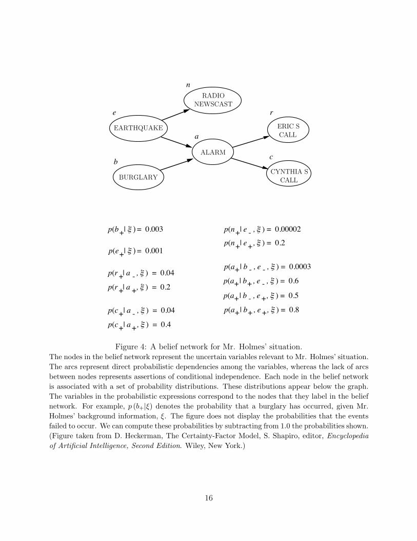
Figure 4 shows a belief network for Mr. Holmes’ situation. The belief network is adirected acyclic graph.6 The nodes in the graph correspond to uncertain variables relevantto the problem. For Mr. Holmes, each uncertain variable represents a proposition andthat proposition’s negation. For example, node b in Figure 4 represents the propositionsBURGLARY and NOT BURGLARY (denoted b+ and b−, respectively). In general, an uncertainvariable can represent an arbitrary set of mutually exclusive and exhaustive propositions;we call each proposition an instance of the variable. In the remainder of the discussion, wemake no distinction between the variable x and the node x that represents that variable.

Each variable in a belief network is associated with a set of probability distributions.7

In the Bayesian tradition, these distributions encode the knowledge provider’s beliefs aboutthe relationships among the variables. Mr. Holmes’ probabilities appear below the beliefnetwork in Figure 4.

The arcs in the directed acyclic graph represent direct probabilistic dependencies among

5Other names for belief networks include probabilistic networks, causal networks, and Bayesian networks.6A directed acyclic graph contains no directed cycles. That is, in a directed acyclic graph, we cannot

travel from a node and return to that same node along a nontrivial directed path.7A probability distribution is an assignment of a probability to each instance of a variable.

15

RADIO NEWSCAST

c

a

b

e

n

ERIC�S CALL

ALARM

CYNTHIA�S CALL

r

EARTHQUAKE

BURGLARY

p(b | ξ ) = 0.003+

p(e | ξ ) = 0.001+

p(r | a , ξ ) = 0.04+ -p(r | a , ξ ) = 0.2+ +

p(n | e , ξ ) = 0.00002+ -p(n | e , ξ ) = 0.2+ +

p(a | b , e , ξ ) = 0.0003+ - -p(a | b , e , ξ ) = 0.6+ + -p(a | b , e , ξ ) = 0.5+ - +p(a | b , e , ξ ) = 0.8+ + +p(c | a , ξ ) = 0.04+ -

p(c | a , ξ ) = 0.4+ +

Figure 4: A belief network for Mr. Holmes’ situation.The nodes in the belief network represent the uncertain variables relevant to Mr. Holmes’ situation.The arcs represent direct probabilistic dependencies among the variables, whereas the lack of arcsbetween nodes represents assertions of conditional independence. Each node in the belief networkis associated with a set of probability distributions. These distributions appear below the graph.The variables in the probabilistic expressions correspond to the nodes that they label in the beliefnetwork. For example, p (b+|ξ) denotes the probability that a burglary has occurred, given Mr.Holmes’ background information, ξ. The figure does not display the probabilities that the eventsfailed to occur. We can compute these probabilities by subtracting from 1.0 the probabilities shown.(Figure taken from D. Heckerman, The Certainty-Factor Model, S. Shapiro, editor, Encyclopediaof Artificial Intelligence, Second Edition. Wiley, New York.)

16

the uncertain variables. In particular, an arc from node x to node y reflects an assertion bythe builder of that network that the probability distribution for y may depend on the instanceof the variable x; we say that x conditions y. Thus, a node has a probability distributionfor every instance of its conditioning nodes. (An instance of a set of nodes is an assignmentof an instance to each node in that set.) For example, in Figure 4, ALARM is conditionedby both EARTHQUAKE and BURGLARY. Consequently, there are four probability distribu-tions for ALARM, corresponding to the instances where both EARTHQUAKE and BURGLARYoccur, BURGLARY occurs alone, EARTHQUAKE occurs alone, and neither EARTHQUAKE norBURGLARY occurs. In contrast, RADIO NEWSCAST, ERIC’S CALL, and CYNTHIA’S CALL areeach conditioned by only one node. Thus, there are two probability distributions for eachof these nodes. Finally, EARTHQUAKE and BURGLARY do not have any conditioning nodes,and hence each node has only one probability distribution.

The lack of arcs in a belief network reflects assertions of conditional independence. Forexample, there is no arc from BURGLARY to ERIC’S CALL in Figure 4. The lack of this arcencodes Mr. Holmes’ belief that the probability of receiving Eric’s telephone call from hisneighbor does not depend on whether or not there was a burglary, provided Mr. Holmesknows whether or not the alarm sounded.

Pearl describes the exact semantics of missing arcs [33]. Here, it is important to recognizethat, given any belief network, we can construct the joint probability distribution for thevariables in any belief network from (1) the probability distributions associated with eachnode in the network, and (2) the assertions of conditional independence reflected by the lackof some arcs in the network. The joint probability distribution for a set of variables is thecollection of probabilities for each instance of that set. The distribution for Mr. Holmes’situation is

p (e, b, a, n, r, c|ξ) = p (e|ξ) p (b|ξ) p (a|e, b, ξ) p (n|e, ξ) p (r|a, ξ) p (c|a, ξ) (8)

The probability distributions on the right-hand side of Equation 8 are exactly those distri-butions associated with the nodes in the belief network.

6.1 Getting Answers from Belief NetworksGiven a joint probability distribution over a set of variables, we can compute any conditionalprobability that involves those variables. In particular, we can compute the probability ofany set of hypotheses, given any set of observations. For example, Mr. Holmes undoubtedlywants to determine the probability of BURGLARY (b+) given RADIO NEWSCAST (n+) andERIC’S CALL (r+) and CYNTHIA’S CALL (c+). Applying the rules of probability8 to the jointprobability distribution for Mr. Holmes’ situation, we obtain

p (b+|n+, r+, c+, ξ) =p (b+, n+, r+, c+|ξ)

p (n+, r+, c+|ξ)

8See, for example, [41].

17

=

Pei,ak

p (ei, b+, ak, n+, r+, c+|ξ)P

ei,bj ,akp (ei, bj, ak, n+, r+, c+|ξ)

where ei, bj, and ak denote arbitrary instances of the variables e, b, and a, respectively.In general, given a belief network, we can compute any set of probabilities from the

joint distribution implied by that network. We also can compute probabilities of interestdirectly within a belief network. In doing so, we can take advantage of the assertions ofconditional independence reflected by the lack of arcs in the network: Fewer arcs lead toless computation. Several researchers have developed an algorithm in which we reversearcs in the belief network, applying Bayes’ theorem to each reversal, until we have derivedthe probabilities of interest [22, 30, 35]. Pearl has developed a message-passing schemethat updates the probability distributions for each node in a belief network in response toobservations of one or more variables [32]. Lauritzen and Spiegelhalter have created analgorithm that first builds an undirected graph from the belief network [26]. The algorithmthen exploits several mathematical properties of undirected graphs to perform probabilisticinference. Most recently, Cooper has developed an inference algorithm that recursivelybisects a belief network, solves the inference subproblems, and reassembles the componentsolutions into a global solution [5].

6.2 Belief Networks for Knowledge AcquisitionA belief network simplifies knowledge acquisition by exploiting a fundamental observationabout the ability of people to assess probabilities. Namely, a belief network takes advantageof the fact that people can make assertions of conditional independence much more easilythan they can assess numerical probabilities [22, 32]. In using a belief network, a personfirst builds the graph that reflects his assertions of conditional independence; only then doeshe assess the probabilities underlying the graph. Thus, a belief network helps a person todecompose the construction of a joint probability distribution into the construction of a setof smaller probability distributions.

6.3 Advantages of the Belief Network over the CF ModelThe example of Mr. Holmes illustrates the advantages of the belief network over the CFmodel. First, we can avoid the practical problem of the CF model that we discussed in Sec-tion 5; namely, using a belief network, a knowledge provider can choose the order in whichhe prefers to assess probability distributions. For example, in Figure 4, all arcs point fromcause to effect, showing that Mr. Holmes prefers to assess the probability of observing aneffect, given one or more causes. If, however, Mr. Holmes wanted to specify the probabilitiesof—say—EARTHQUAKE given RADIO NEWSCAST and of EARTHQUAKE given NOT RADIONEWSCAST, he simply would reverse the arc from RADIO NEWSCAST to EARTHQUAKE inFigure 4. Regardless of the direction in which Mr. Holmes assesses the conditional distri-butions, we can use one of the algorithms mentioned in Section 6.1 to reveal the conditionalprobabilities of interest, if the need arises. (See [36], for a detailed discussion of this point.)

18

Second, using a belief network, the knowledge provider can control the assertions of con-ditional independence that are encoded in the representation. In contrast, the use of thecombination functions in the CF model forces a person to adopt assertions of conditional in-dependence that may be incorrect. For example, as we discussed in Section 4.3, the inferencenetwork in Figure 2 dictates the erroneous assertion that EARTHQUAKE and BURGLARY areconditionally independent, given ALARM.

Third, and most important, a knowledge provider does not have to assess indirect inde-pendencies, using a belief network. Such independencies reveal themselves in the courseof probabilistic computations within the network.9 Such computations can tell us—forexample—that BURGLARY and RADIO NEWSCAST are normally independent, but becomedependent, given ERIC’S CALL, CYNTHIA’S CALL, or both.

Thus, the belief network helps us to tame the inherently nonmodular properties of un-certain reasoning. Uncertain knowledge encoded in a belief network is not as modular as isknowledge about logical relationships. Nonetheless, representing uncertain knowledge in abelief network is a great improvement over encoding all relationships among a set of variables.

6.4 Belief Networks in Real-World ApplicationsDespite the strong theoretical arguments that favor the use of belief networks for representinguncertainty in medical decision-support systems, it is appropriate to ask whether there arepractical technologic approaches to their adoption. Indeed, the belief-network representationrecently has facilitated the construction of several real-world expert systems. For example,researchers at Stanford University and the University of Southern California used a beliefnetwork to construct Pathfinder, an expert system that assists pathologists with the diagnosisof lymph-node diseases [9, 11]. The program reasons about over 60 diseases (25 benigndiseases, 9 Hodgkin’s lymphomas, 18 non-Hodgkin’s lymphomas, and 10 metastatic diseases)and over 140 features of disease, including morphologic, clinical, laboratory, immunological,and molecular biological findings. The belief network for Pathfinder was constructed withthe aid of a similarity network, an extension of the belief-network representation that permitsthe incremental construction of extremely large belief networks from cognitively manageablesubproblems that involve the comparison of two diseases and their distinguishing features[14, 15, 16]. A formal evaluation of Pathfinder has demonstrated that its diagnostic accuracyis at least as good as that of the program’s expert [10]. Currently, the program is undergoingclinical trials that will compare the diagnostic accuracy of general pathologists who haveaccess to Pathfinder to that of pathologists who do not have such access.

Other medical expert systems have been built with belief networks. These systemsinclude Munin, a program for the diagnosis of muscular disorders [2], Alarm, a program thatassists physicians with ventilator management [3], Sleep-It, a program for the diagnosis ofsleep disorders [29], and QMR-DT, a probabilistic version of QMR [39, 27].

In addition to the development of the belief network, there are several changes in com-

9In fact, we are not even required to perform numerical computations to derive such indirect indepen-dencies. An efficient algorithm exists that uses only the structure of the belief network to tell us about thesedependencies [7].

19

puting environments which have been instrumental in making it practical to return to formalprobabilistic models. In particular, the dramatic increase in raw computing power make itreasonable to consider using search algorithms that would have brought reasoning systemsto a halt 20 years ago. Also, the graphical environments that are now routinely availableallow us to address the issues of cognitive complexity that would have limited attempts touse belief networks in earlier decades.

7 ConclusionsThe widespread adoption of the CF model in the late 1970s and early 1980s is clear evidenceof the importance of practical and simple methods for managing uncertain reasoning inexpert systems. As we have seen, however, the simplicity of the CF model was achieved onlywith frequently unrealistic assumptions and with persistent confusion about the meaning ofthe numbers being used.

Fortunately, the belief-network representation overcomes many of the limitations of theCF model, and provides a promising approach to the practical construction of expert systems.We hope that our discussion will inspire investigators to develop belief-network inferencealgorithms and extensions to the representation that will simplify further the constructionand use of probabilistic expert systems. We believe that the time is right for the developmentof such systems in medical domains.

AcknowledgmentsWe thank Bruce Buchanan and Eric Horvitz for many valuable discussions about the CFmodel and its limitations. Mark Peot and Jack Breese provided useful comments on anearlier version of this manuscript. This work was supported by the National Library ofMedicine under the SUMEX-AIM Grant LM05208 and the Pathfinder Grant RO1LM04529,and by the National Cancer Institute under the Pathfinder Grant RO1CA51729-01A1.

References[1] J.B. Adams. A probability model of medical reasoning and the MYCIN model. Math-

ematical Biosciences, 32:177–186, 1976.

[2] S. Andreassen, M. Woldbye, B. Falck, and S.K. Andersen. MUNIN: A causal probabilis-tic network for interpretation of electromyographic findings. In Proceedings of the TenthInternational Joint Conference on Artificial Intelligence, Milan, Italy, pages 366–372.Morgan Kaufmann, San Mateo, CA, August 1987.

[3] I.A. Beinlich, H.J. Suermondt, R.M. Chavez, and G.F. Cooper. The ALARM monitoringsystem: A case study with two probabilistic inference techniques for belief networks. InProceedings of the Second European Conference on Artificial Intelligence in Medicine,London. Springer Verlag, Berlin, August 1989.

20

[4] B.G. Buchanan and E.H. Shortliffe, editors. Rule-Based Expert Systems: The MYCINExperiments of the Stanford Heuristic Programming Project. Addison–Wesley, Reading,MA, 1984.

[5] G.F. Cooper. Bayesian belief-network inference using recursive decomposition. TechnicalReport KSL-90-05, Medical Computer Science Group, Section on Medical Informatics,Stanford University, Stanford, CA, January 1990.

[6] W. Edwards, ed. Special issue on probabilistic inference. IEEE Transactions on HumanFactors in Electronics, 7, 1956.

[7] D. Geiger, T. Verma, and J. Pearl. Identifying independence in Bayesian networks.Networks, 20:507–534, 1990.

[8] I.J. Good. A causal calculus (I). British Journal of Philosophy of Science, 11:305–318, 1961. Also in I.J. Good, Good Thinking: The Foundations of Probability and ItsApplications, pages 197–217. University of Minnesota Press, Minneapolis, MN, 1983.

[9] D. Heckerman, E. Horvitz, and B. Nathwani. Toward normative expert systems: ThePathfinder project. Methods of Information in Medicine, 1991. In press.

[10] D. Heckerman and B. Nathwani. An evaluation of the diagnostic accuracy of Pathfinder.Computers and Biomedical Research, 1991. In press.

[11] D. Heckerman and B. Nathwani. Toward normative expert systems: Probability-basedrepresentations for efficient knowledge acquisition. Methods of Information in Medicine,1991. In press.

[12] D.E. Heckerman. Probabilistic interpretations for MYCIN’s certainty factors. In Pro-ceedings of the Workshop on Uncertainty and Probability in Artificial Intelligence, LosAngeles, CA, pages 9–20. Association for Uncertainty in Artificial Intelligence, Moun-tain View, CA, August 1985. Also in Kanal, L. and Lemmer, J., editors, Uncertaintyin Artificial Intelligence, pages 167–196. North-Holland, New York, 1986.

[13] D.E. Heckerman. Formalizing heuristic methods for reasoning with uncertainty. Tech-nical Report KSL-88-07, Medical Computer Science Group, Section on Medical Infor-matics, Stanford University, Stanford, CA, May 1987.

[14] D.E. Heckerman. Probabilistic similarity networks. Networks, 20:607–636, 1990.

[15] D.E. Heckerman. Probabilistic Similarity Networks. PhD thesis, Program in MedicalInformation Sciences, Stanford University, Stanford, CA, June 1990. Report STAN-CS-90-1316.

[16] D.E. Heckerman. Probabilistic Similarity Networks. MIT Press, Cambridge, MA, 1991.

21

[17] D.E. Heckerman and E.J. Horvitz. The myth of modularity in rule-based systems. InProceedings of the Second Workshop on Uncertainty in Artificial Intelligence, Philadel-phia, PA, pages 115–121. Association for Uncertainty in Artificial Intelligence, MountainView, CA, August 1986. Also in Kanal, L. and Lemmer, J., editors, Uncertainty in Ar-tificial Intelligence 2, pages 23–34. North-Holland, New York, 1988.

[18] D.E. Heckerman and E.J. Horvitz. On the expressiveness of rule-based systems forreasoning under uncertainty. In Proceedings AAAI-87 Sixth National Conference onArtificial Intelligence, Seattle, WA, pages 121–126. AAAI Press, Menlo Park, CA, July1987.

[19] M. Henrion. Should we use probability in uncertain inference systems? In Proceedingsof the Cognitive Science Society Meeting, Amherst, PA. Carnegie–Mellon, August 1986.

[20] M. Henrion. Uncertainty in artificial intelligence: Is probability epistemologically andheuristically adequate? In J.L. Mumpower, editor, Expert Judgment and Expert Sys-tems, pages 105–130. Springer-Verlag, Berlin, Heidelberg, 1987.

[21] E.J. Horvitz, J.S. Breese, and M. Henrion. Decision theory in expert systems andartificial intelligence. International Journal of Approximate Reasoning, 2:247–302, 1988.

[22] R.A. Howard and J.E. Matheson. Influence diagrams. In R.A. Howard and J.E. Math-eson, editors, Readings on the Principles and Applications of Decision Analysis, vol-ume II, pages 721–762. Strategic Decisions Group, Menlo Park, CA, 1981.

[23] R. Johnson. Independence and Bayesian updating methods. In Proceedings of theWorkshop on Uncertainty and Probability in Artificial Intelligence, Los Angeles, CA,pages 28–30. Association for Uncertainty in Artificial Intelligence, Mountain View, CA,August 1985. Also in Kanal, L. and Lemmer J., editors, Uncertainty in Artificial Intel-ligence, pages 197–201. North-Holland, New York, 1986.

[24] D. Kahneman, P. Slovic, and A. Tversky, editors. Judgment Under Uncertainty: Heuris-tics and Biases. Cambridge University Press, New York, 1982.

[25] J.H. Kim and J. Pearl. A computational model for causal and diagnostic reasoning ininference engines. In Proceedings Eighth International Joint Conference on ArtificialIntelligence, Karlsruhe, West Germany, pages 190–193. International Joint Conferenceon Artificial Intelligence, ?? 1983.

[26] S.L. Lauritzen and D.J. Spiegelhalter. Local computations with probabilities on graph-ical structures and their application to expert systems. J. Royal Statistical Society B,50:157–224, 1988.

[27] B. Middleton, M. Shwe, D. Heckerman, M. Henrion, E. Horvitz, H. Lehmann, andG. Cooper. Probabilistic diagnosis using a reformulation of the INTERNIST-1/QMRknowledge base—part 2: Evaluation of diagnostic performance. Methods in Informationand Medicine, 1991. In press.

22

[28] R.A. Miller, E.P. Pople, and J.D. Myers. INTERNIST-1: An experimental computer-based diagnostic consultant for general internal medicine. New England Journal ofMedicine, 307:476–486, 1982.

[29] G. Nino-Murcia and M. Shwe. An expert system for diagnosis of sleep disorders. InM. Chase, R. Lydic, and C. O’Connor, editors, Sleep Research, volume 20, page 433.Brain Information Service, Los Angeles, CA, 1991.

[30] S.M. Olmsted. On Representing and Solving Decision Problems. PhD thesis, Depart-ment of Engineering-Economic Systems, Stanford University, Stanford, CA, December1983.

[31] J. Pearl. Reverend Bayes on inference engines: A distributed hierarchical approach. InProceedings AAAI-82 Second National Conference on Artificial Intelligence, Pittsburgh,PA, pages 133–136. AAAI Press, Menlo Park, CA, August 1982.

[32] J. Pearl. Fusion, propagation, and structuring in belief networks. Artificial Intelligence,29:241–288, 1986.

[33] J. Pearl. Probabilistic Reasoning in Intelligent Systems: Networks of Plausible Inference.Morgan Kaufmann, San Mateo, CA, 1988.

[34] W.F. Rousseau. A method for computing probabilities in complex situations. TechnicalReport 6252-2, Center for Systems Research, Stanford University, Stanford, CA, May1968.

[35] R.D. Shachter. Probabilistic inference and influence diagrams. Operations Research,36:589–604, 1988.

[36] R.D. Shachter and D.E. Heckerman. Thinking backward for knowledge acquisition. AIMagazine, 8:55–63, 1987.

[37] E.H. Shortliffe. Computer-based Medical Consultations: MYCIN. North-Holland, NewYork, 1976.

[38] E.H. Shortliffe and B.G. Buchanan. A model of inexact reasoning in medicine. Mathe-matical Biosciences, 23:351–379, 1975.

[39] M. Shwe, B. Middleton, D. Heckerman, M. Henrion, E. Horvitz, H. Lehmann, andG. Cooper. Probabilistic diagnosis using a reformulation of the INTERNIST-1/QMRknowledge base—part 1: The probabilistic model and inference algorithms. Methods inInformation and Medicine, 1991. In press.

[40] C.S. Spetzler and C.S. Stael von Holstein. Probability encoding in decision analysis.Management Science, 22:340–358, 1975.

[41] M. Tribus. Rational Descriptions, Decisions, and Designs. Pergamon Press, New York,1969.

23

[42] A. Tversky and D. Kahneman. Judgment under uncertainty: Heuristics and biases.Science, 185:1124–1131, 1974.

[43] A. Tversky and D. Kahneman. Causal schemata in judgments under uncertainty.In D. Kahneman, P. Slovic, and A. Tversky, editors, Judgement Under Uncertainty:Heuristics and Biases. Cambridge University Press, New York, 1982.

[44] W. van Melle. A domain-independent system that aids in constructing knowledge-basedconsultation programs. PhD thesis, Department of Computer Science, Stanford Univer-sity, 1980. Report STAN-CS-80-820 and HPP-80-22. Reprinted as van Melle, 1981.

[45] W. van Melle. System Aids in Constructing Consultation Programs. UMI ResearchPress, Ann Arbor, MI, 1981.

[46] S. Wright. Correlation and causation. Journal of Agricultural Research, 20:557–85,1921.

[47] V.L. Yu, B.G. Buchanan, E.H. Shortliffe, S.M. Wraith, R. Davis, A.C. Scott, and S.N.Cohen. Evaluating the performance of a computer-based consultant. Computer Pro-grams in Biomedicine, 9:95–102, 1979.

[48] V.L. Yu, L.M. Fagan, S.M. Wraith, W.J. Clancey, A.C. Scott, J.F. Hannigan, R.L. Blum,B.G. Buchanan, and S.N. Cohen. Antimicrobial selection by a computer: A blindedevaluation by infectious disease experts. Journal of the American Medical Association,242:1279–1282, 1979.

24