from candles to light - microsoft

From Candles to Light:

The Impact of Rural Electrification

Irani Arraiz Carla Calero

Multilateral Investment Fund

IDB-WP-599IDB WORKING PAPER SERIES No.

Inter-American Development Bank

May 2015

From Candles to Light:

The Impact of Rural Electrification

Irani Arraiz Carla Calero

2015

Inter-American Development Bank

Cataloging-in-Publication data provided by the Inter-American Development Bank Felipe Herrera Library Arraiz, Irani. From candles to light: the impact of rural electrification / Irani Arraiz, Carla Calero. p. cm. — (IDB Working Paper Series ; 599) Includes bibliographic references. 1. Rural electrification—Evaluation—Peru. 2. Solar energy—Evaluation—Peru. I. Calero León, Carla . II. Inter-American Development Bank. Multilateral Investment Fund. III. Title. IV. Series. IDB-WP-599

http://www.iadb.org

Any dispute related to the use of the works of the IDB that cannot be settled amicably shall be submitted to arbitration pursuant to the UNCITRAL rules. The use of the IDB’s name for any purpose other than for attribution, and the use of IDB’s logo shall be subject to a separate written license agreement between the IDB and the user and is not authorized as part of this CC-IGO license.

Following a peer review process, and with previous written consent by the Inter-American Development

2015Copyright © Inter-American Development Bank. This work is licensed under a Creative Commons

IGO 3.0 Attribution-NonCommercial-NoDerivatives (CC-IGO BY-NC-ND 3.0 IGO) license (http://creative-commons.org/licenses/by-nc-nd/3.0/igo/legalcode) and may be reproduced with attribution to the IDB and for any non-commercial purpose. No derivative work is allowed.

Bank (IDB), a revised version of this work may also be reproduced in any academic journal, including those indexed by the American Economic Association’s EconLit, provided that the IDB is credited and that the author(s) receive no income from the publication. Therefore, the restriction to receive income from such publication shall only extend to the publication’s author(s). With regard to such restriction, in case of any inconsistency between the Creative Commons IGO 3.0 Attribution-NonCommercial-NoDerivatives license and these statements, the latter shall prevail.

Note that link provided above includes additional terms and conditions of the license.

The opinions expressed in this publication are those of the authors and do not necessarily reflect the views of the Inter-American Development Bank, its Board of Directors, or the countries they represent.

From Candles to Light: The Impact of Rural Electrification ∗

Irani Arraiz† Carla Calero ‡

October 2014

Abstract

This paper studies the impact of access to electricity via solar-powered home systems(SHSs) in rural communities in Peru. Applying propensity score matching at the commu-nity as well as at the household level, the authors find that households with SHSs spendless on traditional sources of energy—candles and batteries for flashlights—and that thesubsequent savings are commensurate to the fee for SHS use. People in households withSHSs spend more time awake, and women in particular change patterns of time use: theyspend more time taking care of children, cooking, doing laundry, and weaving for theirfamilies, and less time in productive activities outside their homes (farming). Childrenspend more time doing homework, which has translated into more years of schooling(among elementary school students) and higher rates of enrollment (in secondary school).Although women spend less time farming and men more time on home business activitiesin households with SHSs than in those without, these changes have had no evident impacton income or poverty.

JEL Classification: D04, I31, Q42, O12.

Keywords: Rural electricity, impact evaluation, solar-powered home systems, Peru.

∗This study was coordinated and financed by the Multilateral Investment Fund (MIF) of the Inter-AmericanDevelopment Bank (IDB). The authors are grateful to ACCIONA Microenergıa Peru (AMP) and the InstitutoNacional de Estadısticas e Informatica (the Peruvian Office of Statistics), for their support in conductingthe study. We also thank Martin Litwar for his research assistance and Instituto Cuanto for excellent datacollection. The views presented in this paper are those of the authors; no endorsement by the Inter-AmericanDevelopment Bank, its Board of Executive Directors, or the countries they represent is expressed or implied.

†Inter-American Development Bank. E-mail: [email protected]‡Inter-American Development Bank. E-mail: [email protected]

1 Introduction

Electricity alone is not sufficient to spur economic growth, but it is certainly necessary. Accessto electricity is crucial to human development: electricity is indispensable for basic activitiesthat many in the world take for granted—lighting, refrigeration, and the running of householdappliances. It is an alarming fact that, even today, hundreds of millions of people lack accessto the most basic energy services. According to the International Energy Agency (IEA 2014)an estimated 1.3 billion people lacked access to electricity in 2014; this is nearly one-fifth ofthe worlds population.

The majority of those without electricity live in rural areas, but there are large variationsin electrification rates across and within regions. The relatively high average access rates incertain regions mask problems in some subregions and individual countries. In Latin America,for example, where the electrification rate is 95 percent overall, there is the extreme case ofHaiti, which has an overall electrification rate of 28 percent and a mere 9 percent in ruralareas. In Peru the electrification rate reaches as high as 90 percent, but in rural areas suchas Cajamarca this rate is only 18 percent—the countrys lowest rate. In some districts withinCajamarca up to 96 percent of the population lives without access to electricity.

Providing people in rural areas with access to electrification is a challenge. Most ruralcommunities, as well as many peri-urban areas, are characterized by low population densityand a disproportionately high percentage of poor households. Demand for electricity is oftenlimited to residential and agricultural consumers; households that use electricity consume,on average, less than 30 kilowatt-hours (kWh) per month—and this is generally during peakevening hours. As a result, rural electricity systems invariably have much higher investmentcosts per client and per kilowatt-hour of sales than urban systems. Where the costs of reach-ing distant communities exceed a certain threshold level, it becomes cheaper to use off-gridsources of supply—mini grids served by mini hydro plants or diesel units, and solar home orcommunity systems. But off-grid electrification faces the same challenge that may discouragegrid extension into rural areas: high costs amid low demand.

The high costs of electricity supply in rural areas and the limited capacity of households topay for service make it difficult to attract investment in rural electrification. A well-plannedsystem of tariffs and subsidies must ensure sustainable cost-recovery while minimizing pricedistortions. To be financially sustainable, the utility companies serving poor, rural populationsmust match the costs of efficiently run service providers; any supplement to revenues receivedfrom consumers via subsidy funds should go to support efficiently run service providers; anysupplement to revenues received from consumers via subsidy funds should go to supportefficiently managed utility companies to avoid wasting public funds.

Strong institutions are needed to carefully plan and define the selection criteria for ruralelectrification projects, while regulatory procedures must be tailored to specific contexts.Challenges abound, including the need for sufficient technical and managerial capabilities,power generation, and the capacity to serve the existing grid-connected demand.

Despite these challenges, the need to increase access is widely recognized. Modern energyservices enhance the life of the poor in countless ways. Electricity provides the best andmost efficient form of lighting, extending the day and providing extra hours to study or work.Household appliances also require electricity, opening up new possibilities for communication,entertainment, heating, and so on. Electricity enables water to be pumped for crops, andfood and medicine to be refrigerated. And modern energy can directly reduce poverty byraising a poor countrys productivity and extending the quality and range of its products—

1

thereby putting more wages into the pockets of the deprived. For instance, mechanical powercan benefit agriculture (plowing and irrigation), food processing (otherwise, a laborious andtime-consuming job), textiles, and manufacturing.

There is broad consensus in the research literature that rural electrification programsbenefit consumers. But as Ravallion (2008) documents, many early papers suffer from a lack ofmethodological rigor that does not allow correlation and causation to be distinguished. A goodnumber of recent papers, however—Khandker, Barnes, and Samad (2013); Chakravorty, Pelli,and Marchand (2014); Gonzalez and Rossi (2006); and Dinkelman (2011), among others—have used more robust econometric techniques to establish a clearer causal link betweenelectrification and variables of interest.

Khandker, Barnes, and Samad (2009; 2013) examine the impact of connecting rural com-munities to the grid in Bangladesh and Vietnam, respectively. Both studies provide credibleevidence that rural electrification boosts the income, expenditure, and education outcomesof households. The authors tackle the issue of causality by employing robust econometrictechniques, such as propensity score matching (PSM), instrumental variables, and difference-in-differences (DID) to address endogeneity concerns. In Bangladesh the authors (2009) findan increase in annual per capita expenditure of 8.2 percent and an increase in annual totalincome of 12.2 percent. They also find that electricity leads to a significant improvementin completed years of schooling (0.13 years for girls) and study time for children in ruralhouseholds—six more minutes for boys and nine more minutes for girls per day. In Vietnamthe same authors (2013) find an increase in household income of 28 percent and an increase ofhousehold expenditure of 23 percent due to electrification. Household electrification increasesschool attendance by 6.3 percentage points (pp) for boys and 9.0 pp for girls. Communeelectrification increases years of schooling—0.13 years for boys and 0.90 years for girls—forchildren aged 518.

Aguirre (2014), using an instrumental variable approach, finds that providing householdswith access to electricity in Peru boosts childrens study time by an extra 93 minutes per day.He uses the topographic distance between the population center and the nearest medium-voltage line as an instrument: this distance is correlated with a households likelihood of beingconnected to the grid but not with the study time of children at home.

Using a natural experiment in Argentina, Gonzalez and Rossi (2006) find evidence thatproviding access to a high-quality supply of electricity reduces the frequency of low birthweight (by 20 percent relative to the baseline proportion of 1 child in 100) and child mortalityrates in children under five years of age caused by diarrhea and food poisoning (by 33.2percent relative to the baseline proportion of 25 children in 10,000). The authors arguethat electrified households ability to own a refrigerator—and reductions in the frequency andduration of blackouts—reduces the likelihood of food poisoning and increases the variety andquality of the mothers diet by improving her micronutrient consumption.

Dinkelman (2011) investigates the impact of domestic electrification on employment inrural South Africa, where in 1993—a year before the end of apartheid—more than 80 percentof households relied on wood for basic energy needs. By 2001, 2 million households werenewly connected to the grid. Newly electrified communities have shifted away from usingwood at home, toward electric cooking and lighting. Household electrification has operatedas a labor-saving technology, releasing womens time spent in household work to allow themmore productivity in the market. By exploiting community-level variation in the timingof electrification, results show that female employment rose by a significant 9 to 9.5 pp intreated areas, while the change in the male employment rate was not statistically significant.

2

Electrification increased employment for women on the extensive as well as on the intensivemargin: women worked about 8.9 more hours per week in treated communities. These positive,significant changes for women are notable, since over the same period, national employmentrates fell.

In a recent paper Chakravorty, Pelli, and Marchand (2014) examine not only the effect ofgrid connection, but also the quality of power supply on household incomes in rural India. Theauthors find that grid connection increased the nonagricultural incomes of rural householdsby about 9 percent during the study period 19942005. Moreover, higher-quality electricity—in terms of fewer outages and more hours of electricity per day—increased nonagriculturalincomes by about 29 percent during the same period. This highlights the importance ofproviding high-quality power; the potential benefits of electricity are not realized by onlyconnecting households to the grid.

Rud (2012) investigates the effect of electricity provision on industrialization using a panelof Indian states from 1965 to 1984. To do this and to address the endogeneity of investmentin electrification, he examines the introduction of a new agricultural technology intensive inirrigation. The logic behind his analysis is that as electric pump sets are used to providefarmers with cheap irrigation water, the uneven availability of groundwater can be used topredict divergence in the expansion of the electricity network and, ultimately, to quantify theeffect of electrification on industrial outcomes. Rud also presents a series of tests to rule outalternative explanations that could link groundwater availability to industrialization directlyor through means other than electrification. Overall, he finds that the uneven expansion ofthe electricity network explains between 10 pp and 15 pp of the difference in manufacturingoutput across states in India.

In this paper we use household- and individual-level data to estimate the impact of elec-trification using solar-powered home systems (SHSs) in rural areas in the Department ofCajamarca in Peru. We take advantage of the expansion of the electrification program intoa second set of communities to control for unobservable factors that may affect participationin the program and its impact. Applying PSM at the community as well as at the householdlevel, we find that households with SHSs spend less on traditional sources of energy—candlesand batteries for flashlights—and that the subsequent savings are commensurate to the elec-tricity fee. People in households with SHSs spend more time awake, and women in particularchange their daily patterns: they spend more time taking care of children, cooking, doinglaundry, and weaving for their families and less time in productive activities outside theirhomes (farming). Children spend more time doing homework, which has translated in 0.4more years of schooling (among elementary school children) and higher rates of enrollment(in secondary school).

The main contribution of this paper is to provide further evidence that rural electrifica-tion via SHSs is effective. Similar to other studies, we focus on outcomes such as energyexpenditure, use of time, and outcomes related to education, health, and fertility. Evidenceon solar programs is scarce: most of the literature studies the impact of rural electrificationvia grid connection. This study makes an important, early contribution to a promising topic:expanding electricity access in rural communities by utilizing solar technology.

The rest of the paper is organized as follows: section 2 describes the business model usedby ACCIONA Microenergıa Peru (AMP) to serve local communities, section 3 describes thedataset and presents the model used for the estimation, section 4 presents results, and section5 concludes.

3

2 The Business Model of ACCIONA Microenergıa Peru

ACCIONA Microenergıa Peru (AMP) was created in January 2009 with the objective ofincreasing access to electricity and water in rural communities in the Department of Cajamarcathat were not expected to be connected to the grid in the ensuing years. At the moment itsactivity centers on the provision of electricity.

In August 2009 AMP began the Luz en Casa (Light at Home) program to expand accessto basic electricity services powered by solar-powered home systems (SHSs). The programoperates in isolated and scattered communities located 3,0004,000 meters above sea level inthe northern mountains of Cajamarca, in the Andes. The program involves beneficiaries inthe installation and operation of SHSs, and collects a fee for service. SHSs have the capacityto generate between 7 and 10 kWh of direct current per month. This provides the power tolight three low-energy bulbs for at least four hours a day, with the possibility of poweringlow-energy consumption appliances such as a TV, radio, and a mobile-phone charger.1,2

The contracts signed between AMP and its clients are for 20 years, equivalent to theduration of photovoltaic (PV) systems, and can be reduced in case the national electric gridreaches the area where the beneficiaries live. The client pays a monthly service fee, whichincludes the rent of the equipment, its maintenance for the next 20 years, and the amortizationof the equipment. Thus, if some component breaks, it can be replaced during the 20 years ofservice. Under this model, the equipment belongs to AMP and the households do not haveto bear the costs of purchasing a SHS, whose investment cost is about $700 in Peru. Themonthly fee of about $3.50 (including taxes) is less than the average monthly energy coststhat the households incurred before the program was implemented.3

When planning where to install SHSs, AMP identifies rural communities that are partof the Peruvian governments Rural Electrification Plan in geographical areas where thereis a potential to deploy PV systems for domestic or communal use. Such areas are eitherinconvenient or impossible to connect to the grid, whether from a technical or economicperspective. AMP coordinates with the national and local government to enable the programsfinancial viability without compromising its focus on low-income populations.

The AMP business model aims to make electricity affordable for low-income populations—and sustainable over time, since the service fee covers any damage to system components. Be-cause the selection of communities is based on the national governments Rural ElectrificationPlan and is agreed upon with local authorities, it is unlikely that AMPs fee-for-service modelwill become financially untenable because the grid is expanded unexpectedly—endangeringthe customer base before the supplier can recover its investment in the equipment. Otherbusiness models where households acquire—and in some cases finance—solar systems havethe downside of making the service less attractive to low-income households. Cash purchasesinvolve a high opportunity cost for low-income families and are less sustainable since any

1The average consumption per capita in Peru was 1,248 kWh in 2011 (World Bank, World DevelopmentIndicators). The household consumption ranges between 53 kWh/month for an average household classified associoeconomic level E (the poorest) and 1,050 kWh a month for an average household classified as socioeconomiclevel A (the wealthiest) (Organismo Supervisor de la Inversion en Energıa, OSINERGMIN). When AMPoffered a system able to generate more power at a higher cost, households expressed a preference for themore-economical, lower-power option.

2Because the system generates direct current (DC) and most appliances use alternate current (AC), house-holds either have to use a power inverter or acquire DC-powered appliances.

3Households’ average energy cost, according to a socioeconomic study conducted by AMP in 2010 of 600households in the area of the program, was $5.07.

4

problem with the system must be paid for by the household.After potential beneficiary communities have been identified, AMP coordinates awareness

meetings with community members to explain its process. If there is enough interest, thecommunity forms a Photovoltaic Electrification Committee (PEC). The committee seeks theactive participation of users and also serves as the main communication vehicle between AMPand the community. The PEC members are elected by and among the beneficiaries themselves.

Prior to the installation of SHSs, AMP trains both PEC members and the users. Duringthe training AMP informs all parties of their rights and duties, presents the capabilities andlimitations of the PV system, and tells users how to respond to problems. The members of thePEC are given intensive training in the operation of the equipment, preventive maintenancetasks (visual inspection and verification of the proper operation of the SHS), and proceduresfor participating in the program (collection of fees, payments to AMP, communication oftechnical failures, inspections, safety, users rights, and commitments to AMP). The trainingis offered during the awareness meetings and at the time of installation. There is also a specifictraining for those users selected as local technicians, who are responsible for the installation(under the supervision of AMP staff) and corrective maintenance of the equipment. Therelationship between the technicians and AMP is regulated by a professional services contract.

The PECs are responsible for collecting users fees, making payments at the AMP head-quarters in Cajamarca, and distributing the corresponding receipts to customers. This man-agement of payments is expensive because it involves, in many cases, the movement of a personfrom the community to Cajamarca, which carries with it the risk of theft. In some commu-nities, the PEC charges an additional, small contribution of about $0.35 that helps cover thetreasurers cost of transportation; additionally, AMP waives the treasurers own service fee.

AMP receives a monthly fee of around $3.50 per household, which accounts for about20 percent of the regulated rate; the difference is borne by the Fondo de CompensacionSocial Electrico (FOSE, for its acronym in Spanish). FOSE is a fund (part of the socialinclusion policy promoted by the Peruvian government) whereby higher-consumption users(who use more than 100 kWh/month) pay a monthly surcharge on their electricity bills tosubsidize the rate of low-consumption users (100 kWh/month or less)—serviced by privateoperators investing in renewable, off-grid power in rural communities. These private investorsmust be authorized by the Supervisory Agency for Investment in Energy and Mining in Peru(Organismo Supervisor de la Inversion en Energıa, OSINERGMIN) to be eligible for thesubsidies.4 Under this cross-subsidy mechanism, FOSE pays about 80 percent of the set rateto AMP, and the user pays only 20 percent.5

This complementary revenue mechanism is key to the fee-for-service business model im-plemented by AMP. It provides incentives for the private sector to carry out investmentsin rural electrification programs using renewable energy, and targets low-income populationswithout jeopardizing the ability of these households to benefit from the service due to highcosts. The subsidy targets low-consumption users in rural communities, served by systemsunder 20 megawatts (MW).

4Organismo Supervisor de la Inversion en Energıa (OSINERGMIN) is the supervisory agency for investmentin energy and mining in Peru. In 2011 AMP was recognized by OSINERGMIN as a public electricity service,making it the main supplier of electricity relying exclusively on SHSs.

5AMP periodically sends all the required documentation to OSINERGMIN to receive the correspondingfunds from Fondo de Compensacion Social Electrico (FOSE). Unlike the fixed rates paid by customers, whatAMP receives from FOSE varies according to the rate published monthly by OSINERGMIN. AMP has decidednot to pass these changes on to its costumers (the rate that users would have to pay in 2014, according to therates published by OSINERGMIN, is slightly more than $3.50).

5

3 Research Methodology

3.1 Data

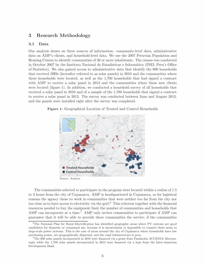
Our analysis draws on three sources of information: community-level data, administrativedata on AMP’s clients, and household-level data. We use the 2007 Peruvian Population andHousing Census to identify communities of 30 or more inhabitants. The census was conductedin October 2007 by the Instituto Nacional de Estadısticas e Informatica (INEI, Peru’s Officeof Statistics). We also gained access to administrative data that identify the 600 householdsthat received SHSs (hereafter referred to as solar panels) in 2010 and the communities wherethese households were located, as well as the 1,700 households that had signed a contractwith AMP to receive a solar panel in 2013 and the communities where these new clientswere located (figure 1). In addition, we conducted a household survey of all households thatreceived a solar panel in 2010 and of a sample of the 1,700 households that signed a contractto receive a solar panel in 2013. The survey was conducted between June and August 2013,and the panels were installed right after the survey was completed.

Figure 1: Geographical Location of Treated and Control Households

Treated Households

Control Households

Source: Authors.

The communities selected to participate in the program were located within a radius of 1.5to 3 hours from the city of Cajamarca. AMP is headquartered in Cajamarca, so for logisticalreasons the agency chose to work in communities that were neither too far from the city nortoo close as to have access to electricity via the grid.6 This criterion together with the financialresources needed to buy the equipment limit the number of communities and households thatAMP can incorporate at a time.7 AMP only invites communities to participate if AMP canguarantee that it will be able to provide these communities the service, if the communities

6The National Plan for Rural Electrification has identified geographic areas where PV systems are goodcandidates for domestic or communal use, because it is inconvenient or impossible to connect these areas tolarge-scale power systems. This is the case of areas around the city of Cajamarca where households have lowpurchasing power, are geographically dispersed, and the road infrastructure is poor.

7The 600 solar panels incorporated in 2010 were financed via a grant from Fundacion ACCIONA Microen-ergıa while the 1,700 solar panels incorporated in 2013 were financed via a loan from the Inter-AmericanDevelopment Bank.

6

choose to participate, in the short term. There are no other criteria—such as the communitypoverty levels—used to select eligible communities.

The sample size was calculated using data from the annual household surveys conducted byINEI, limiting the data to nonelectrified communities located in the districts served by AMP.We set the sample size at 1,320 households (for a statistical power of 0.8 and a significancelevel of 0.05), which allowed us to measure impacts between 0.16 and 0.21 standard deviationsfor continuous variables and between 8 and 10.5 pp for discrete variables depending on theassumptions used for intercluster correlation.

3.2 Identification Strategy

We sought to estimate the impact of access to electricity—via solar panels—on householdmembers’ well-being, as measured by (i) spending on traditional sources of energy, (ii) useof time, (iii) education, and (iv) income (that is, the average impact of treatment on thetreated, ATT). The causal effect of the program is the difference between the mean value ofthe outcome variable in two different scenarios: one in which the household participates inthe program and one in which it does not. The main difficulty in estimating this causal effectis that households cannot simultaneously participate and not participate in the program, andtherefore it is necessary to construct a counterfactual.

When the treatment is assigned randomly, the counterfactual is easily estimated by av-eraging the value of the outcome variable for the nontreated. But when the treatment isnot randomly assigned, as in our case, participants and nonparticipants may differ in theircharacteristics—both observable and unobservable. Therefore, the simple comparison of aver-ages between participants and nonparticipants does not provide an unbiased estimate for thecausal effect. Moreover, it may be precisely the difference in those characteristics that explainswhy some households decide to participate in the program and others do not. Therefore, toidentify the causal effect of the program, it is necessary to consider the effect of observable andunobservable characteristics on both the decision to participate and the outcome variables.

To account for observable characteristics, we use propensity score matching (PSM) tofind, in a group of nonparticipants, those households who are similar to the participantsin all relevant pretreatment characteristics. There are several alternative ways to matchparticipants and nonparticipants and, in general, results depend on the matching algorithmand the variables included to estimate the propensity score.

We carried out two matching exercises. The first matching exercise uses data from the2007 census at the community level to select, from the list of communities to receive servicein 2013, the control community where we interviewed households that had signed a contractwith AMP to get a solar panel in 2013. The second matching exercise uses data from thehousehold survey to match households using a panel since 2010 with households that weregoing to get a panel installed immediately after the survey was administered between Juneand August 2013. We use temporary invariant variables in the second matching exercise toguarantee that household and individual characteristics were identical before the treatment.We match observations using the kernel algorithm with a small, uniform bandwidth in thecommon support. This approach lowers the variance, and the quality of the matching iscontrolled using a small bandwidth (Caliendo and Kopening 2008; Heinrich, Maffioli, andVazquez 2010).

But matching methods are not robust against hidden bias that arises from the existence ofunobserved variables that simultaneously affect assignment to the treatment and the outcome

7

variable. We address these issues by considering only households that either signed a contractto get the service from AMP in 2010 (treated) or households that signed a contract to get theservice in 2013 (controls) in communities being offered the service for the first time.8 Thissuggests that these households share some unobservable characteristics. We also conductedsensitivity analysis to determine how strong an unmeasurable variable must be to influencethe selection process so as to undermine the implications of the analysis.

After identifying the households in the control group (that is, nonbeneficiaries with thesame probability of participation as beneficiaries), it was necessary to check that the observ-able characteristics of the control group were equal to the characteristics of the treatmentgroup (those households that participated in the program in the first round of solar panelinstallation) (Rosenbaum and Rubin 1983). We tested this by: (i) a difference in mean testbefore and after the matching; and (ii) a joint test to ensure that all the characteristics in thecontrol group were equal in mean to those in the treatment group.

We estimated the impact of the program by estimating the parameters τT in the followingequation:

τT =1

NT

∑

i∈T

(Y 1i − Y 0

i ) (1)

Where:

Y 1i =

Yi if Zi = 11

#M (i)

∑

j∈M (i)

Yj if Zi = 0

Y 0i =

Yi if Zi = 01

#M (i)

∑

j∈M (i)

Yj if Zi = 1

and Zi is the treatment indicator for each unit i = 1, ...N ; Yi is the potential outcomefor unit i; and M (i) is the set of indices for the #M(i) matches for unit i found around thebandwidth defined in the algorithm.

We calculate bootstrapped standard errors for the estimates to account for the two stepmatching procedure. Because the kernel-based matching estimator is asymptotically linear,the bootstrap provides a valid inference for the standard errors (Abadie and Imbens, 2008).

4 Results

4.1 Participation Model

As mentioned above, we estimate the effect of the program using matching methods. Thebalance in the observable characteristics of the first matching exercise, intended to select thecommunities to be used as controls from the list of communities to be served in 2013, ispresented in table 1. In general, the census variables do not display statistically significantdifferences in mean values. Only in a few cases are differences obvious: wall materials, orthe presence of a radio, TV, or cell phone. This evidence reflects that the preinterventioncharacteristics of the control and treated communities that resulted from the matching exerciseare similar.

8Some households that signed the contract in 2013 were located in communities where AMP was extendingthe service initially provided in 2010.

8

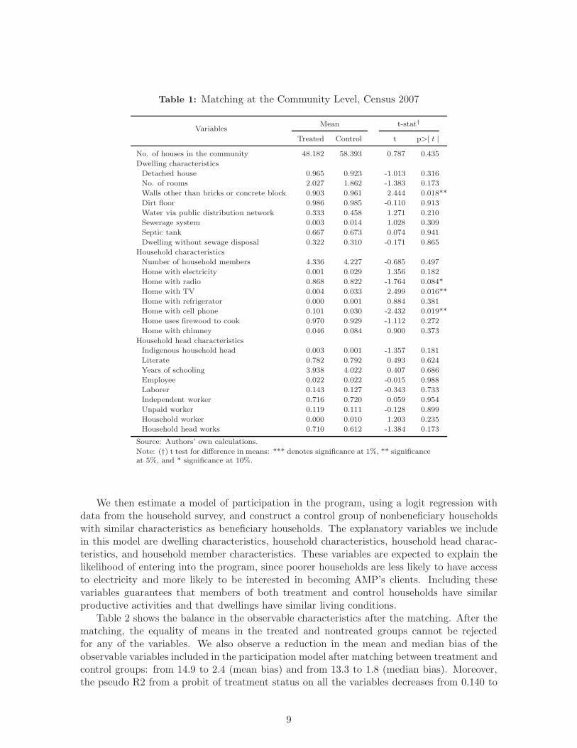
Table 1: Matching at the Community Level, Census 2007

VariablesMean t-stat†

Treated Control t p>| t |

No. of houses in the community 48.182 58.393 0.787 0.435

Dwelling characteristics

Detached house 0.965 0.923 -1.013 0.316

No. of rooms 2.027 1.862 -1.383 0.173

Walls other than bricks or concrete block 0.903 0.961 2.444 0.018**

Dirt floor 0.986 0.985 -0.110 0.913

Water via public distribution network 0.333 0.458 1.271 0.210

Sewerage system 0.003 0.014 1.028 0.309

Septic tank 0.667 0.673 0.074 0.941

Dwelling without sewage disposal 0.322 0.310 -0.171 0.865

Household characteristics

Number of household members 4.336 4.227 -0.685 0.497

Home with electricity 0.001 0.029 1.356 0.182

Home with radio 0.868 0.822 -1.764 0.084*

Home with TV 0.004 0.033 2.499 0.016**

Home with refrigerator 0.000 0.001 0.884 0.381

Home with cell phone 0.101 0.030 -2.432 0.019**

Home uses firewood to cook 0.970 0.929 -1.112 0.272

Home with chimney 0.046 0.084 0.900 0.373

Household head characteristics

Indigenous household head 0.003 0.001 -1.357 0.181

Literate 0.782 0.792 0.493 0.624

Years of schooling 3.938 4.022 0.407 0.686

Employee 0.022 0.022 -0.015 0.988

Laborer 0.143 0.127 -0.343 0.733

Independent worker 0.716 0.720 0.059 0.954

Unpaid worker 0.119 0.111 -0.128 0.899

Household worker 0.000 0.010 1.203 0.235

Household head works 0.710 0.612 -1.384 0.173

Source: Authors’ own calculations.

Note: (†) t test for difference in means: *** denotes significance at 1%, ** significanceat 5%, and * significance at 10%.

We then estimate a model of participation in the program, using a logit regression withdata from the household survey, and construct a control group of nonbeneficiary householdswith similar characteristics as beneficiary households. The explanatory variables we includein this model are dwelling characteristics, household characteristics, household head charac-teristics, and household member characteristics. These variables are expected to explain thelikelihood of entering into the program, since poorer households are less likely to have accessto electricity and more likely to be interested in becoming AMP’s clients. Including thesevariables guarantees that members of both treatment and control households have similarproductive activities and that dwellings have similar living conditions.

Table 2 shows the balance in the observable characteristics after the matching. After thematching, the equality of means in the treated and nontreated groups cannot be rejectedfor any of the variables. We also observe a reduction in the mean and median bias of theobservable variables included in the participation model after matching between treatment andcontrol groups: from 14.9 to 2.4 (mean bias) and from 13.3 to 1.8 (median bias). Moreover,the pseudo R2 from a probit of treatment status on all the variables decreases from 0.140 to

9

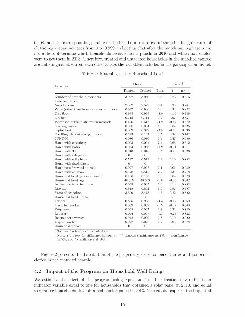
0.008, and the corresponding p-value of the likelihood-ratio test of the joint insignificance ofall the regressors increases from 0 to 0.999, indicating that after the match our regressors arenot able to determine which households received solar panels in 2010 and which householdswere to get them in 2013. Therefore, treated and untreated households in the matched sampleare indistinguishable from each other across the variables included in the participation model.

Table 2: Matching at the Household Level

VariablesMean t-stat†

Treated Control %bias t p>| t |

Number of household members 3.992 3.960 1.8 0.23 0.816

Detached house 1 1 . . .

No. of rooms 2.552 2.522 2.4 0.33 0.741

Walls (other than bricks or concrete block) 0.997 0.996 1.6 0.22 0.822

Dirt floor 0.995 0.999 -4.9 -1.16 0.248

Kitchen 0.745 0.714 7.2 0.97 0.331

Water via public distribution network 0.496 0.517 -4.2 -0.57 0.572

Sewerage system 0.008 0.004 3.8 0.64 0.525

Septic tank 0.879 0.892 -3.5 -0.53 0.596

Dwelling without sewage disposal 0.113 0.104 2.5 0.38 0.702

JUNTOS 0.086 0.076 3.4 0.47 0.639

Home with electricity 0.003 0.001 2.4 0.66 0.512

Home with radio 0.954 0.956 -0.9 -0.11 0.911

Home with TV 0.043 0.046 -1.7 -0.22 0.826

Home with refrigerator 0 0 . . .

Home with cell phone 0.517 0.511 1.4 0.19 0.852

Home with fixed phone 0 0 . . .

Home uses firewood to cook 0.997 0.997 0.1 0.01 0.989

Home with chimney 0.528 0.515 2.7 0.36 0.718

Household head gender (female) 0.166 0.165 0.3 0.04 0.970

Household head age 48.319 48.609 -1.8 -0.25 0.802

Indigenous household head 0.005 0.005 0.6 0.14 0.892

Literate 0.828 0.802 6.9 0.92 0.357

Years of schooling 3.509 3.473 1.6 0.22 0.822

Household head works 1 1 . . .

Farmer 0.895 0.908 -4.3 -0.57 0.569

Unskilled worker 0.059 0.062 -1.3 -0.17 0.868

Employee 0.008 0.007 1.3 0.22 0.830

Laborer 0.054 0.057 -1.8 -0.23 0.822

Independent worker 0.912 0.909 0.8 0.10 0.920

Unpaid worker 0.027 0.026 0.2 0.03 0.978

Household worker 0 0 . . .


Note: (†) t test for difference in means: *** denotes significance at 1%, ** significanceat 5%, and * significance at 10%.

Figure 2 presents the distribution of the propensity score for beneficiaries and nonbenefi-ciaries in the matched sample.

4.2 Impact of the Program on Household Well-Being

We estimate the effect of the program using equation (1). The treatment variable is anindicator variable equal to one for households that obtained a solar panel in 2010, and equalto zero for households that obtained a solar panel in 2013. The results capture the impact of

10

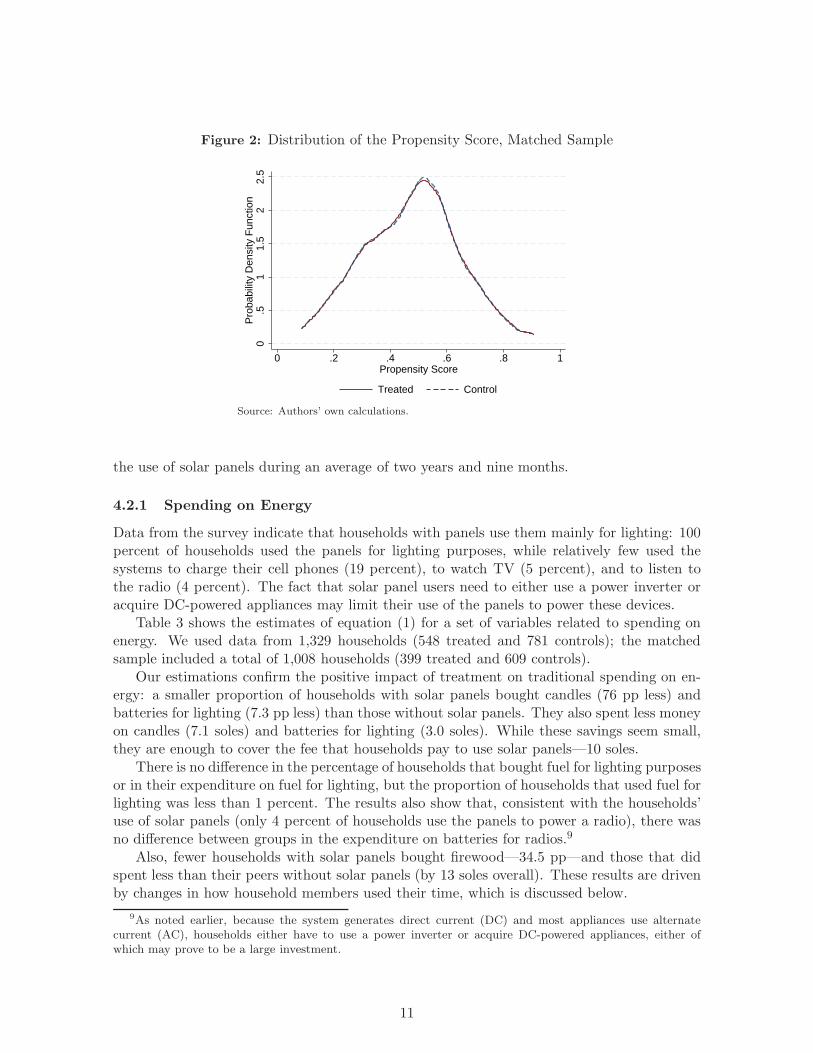
Figure 2: Distribution of the Propensity Score, Matched Sample

0.5

11.

52

2.5

Pro

babi

lity

Den

sity

Fun

ctio

n

0 .2 .4 .6 .8 1Propensity Score

Treated Control


the use of solar panels during an average of two years and nine months.

4.2.1 Spending on Energy

Data from the survey indicate that households with panels use them mainly for lighting: 100percent of households used the panels for lighting purposes, while relatively few used thesystems to charge their cell phones (19 percent), to watch TV (5 percent), and to listen tothe radio (4 percent). The fact that solar panel users need to either use a power inverter oracquire DC-powered appliances may limit their use of the panels to power these devices.

Table 3 shows the estimates of equation (1) for a set of variables related to spending onenergy. We used data from 1,329 households (548 treated and 781 controls); the matchedsample included a total of 1,008 households (399 treated and 609 controls).

Our estimations confirm the positive impact of treatment on traditional spending on en-ergy: a smaller proportion of households with solar panels bought candles (76 pp less) andbatteries for lighting (7.3 pp less) than those without solar panels. They also spent less moneyon candles (7.1 soles) and batteries for lighting (3.0 soles). While these savings seem small,they are enough to cover the fee that households pay to use solar panels—10 soles.

There is no difference in the percentage of households that bought fuel for lighting purposesor in their expenditure on fuel for lighting, but the proportion of households that used fuel forlighting was less than 1 percent. The results also show that, consistent with the households’use of solar panels (only 4 percent of households use the panels to power a radio), there wasno difference between groups in the expenditure on batteries for radios.9

Also, fewer households with solar panels bought firewood—34.5 pp—and those that didspent less than their peers without solar panels (by 13 soles overall). These results are drivenby changes in how household members used their time, which is discussed below.

9As noted earlier, because the system generates direct current (DC) and most appliances use alternatecurrent (AC), households either have to use a power inverter or acquire DC-powered appliances, either ofwhich may prove to be a large investment.

11

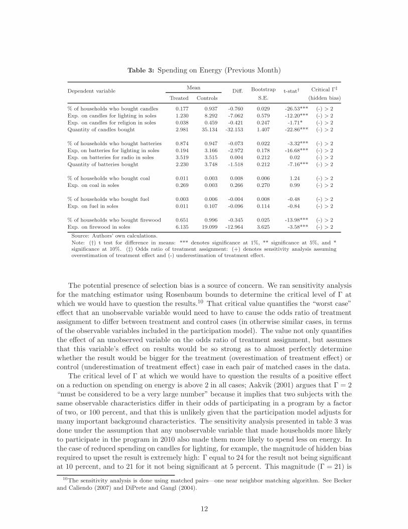
Table 3: Spending on Energy (Previous Month)

Dependent variableMean

Diff. Bootstrap t-stat† Critical Γ‡

Treated Controls S.E. (hidden bias)

% of households who bought candles 0.177 0.937 -0.760 0.029 -26.53*** (-) > 2

Exp. on candles for lighting in soles 1.230 8.292 -7.062 0.579 -12.20*** (-) > 2

Exp. on candles for religion in soles 0.038 0.459 -0.421 0.247 -1.71* (-) > 2

Quantity of candles bought 2.981 35.134 -32.153 1.407 -22.86*** (-) > 2

% of households who bought batteries 0.874 0.947 -0.073 0.022 -3.32*** (-) > 2

Exp, on batteries for lighting in soles 0.194 3.166 -2.972 0.178 -16.68*** (-) > 2

Exp. on batteries for radio in soles 3.519 3.515 0.004 0.212 0.02 (-) > 2

Quantity of batteries bought 2.230 3.748 -1.518 0.212 -7.16*** (-) > 2

% of households who bought coal 0.011 0.003 0.008 0.006 1.24 (-) > 2

Exp. on coal in soles 0.269 0.003 0.266 0.270 0.99 (-) > 2

% of households who bought fuel 0.003 0.006 -0.004 0.008 -0.48 (-) > 2

Exp. on fuel in soles 0.011 0.107 -0.096 0.114 -0.84 (-) > 2

% of households who bought firewood 0.651 0.996 -0.345 0.025 -13.98*** (-) > 2

Exp. on firewood in soles 6.135 19.099 -12.964 3.625 -3.58*** (-) > 2


Note: (†) t test for difference in means: *** denotes significance at 1%, ** significance at 5%, and *significance at 10%. (‡) Odds ratio of treatment assignment: (+) denotes sensitivity analysis assumingoverestimation of treatment effect and (-) underestimation of treatment effect.

The potential presence of selection bias is a source of concern. We ran sensitivity analysisfor the matching estimator using Rosenbaum bounds to determine the critical level of Γ atwhich we would have to question the results.10 That critical value quantifies the “worst case”effect that an unobservable variable would need to have to cause the odds ratio of treatmentassignment to differ between treatment and control cases (in otherwise similar cases, in termsof the observable variables included in the participation model). The value not only quantifiesthe effect of an unobserved variable on the odds ratio of treatment assignment, but assumesthat this variable’s effect on results would be so strong as to almost perfectly determinewhether the result would be bigger for the treatment (overestimation of treatment effect) orcontrol (underestimation of treatment effect) case in each pair of matched cases in the data.

The critical level of Γ at which we would have to question the results of a positive effecton a reduction on spending on energy is above 2 in all cases; Aakvik (2001) argues that Γ = 2“must be considered to be a very large number” because it implies that two subjects with thesame observable characteristics differ in their odds of participating in a program by a factorof two, or 100 percent, and that this is unlikely given that the participation model adjusts formany important background characteristics. The sensitivity analysis presented in table 3 wasdone under the assumption that any unobservable variable that made households more likelyto participate in the program in 2010 also made them more likely to spend less on energy. Inthe case of reduced spending on candles for lighting, for example, the magnitude of hidden biasrequired to upset the result is extremely high: Γ equal to 24 for the result not being significantat 10 percent, and to 21 for it not being significant at 5 percent. This magnitude (Γ = 21) is

10The sensitivity analysis is done using matched pairs—one near neighbor matching algorithm. See Beckerand Caliendo (2007) and DiPrete and Gangl (2004).

12

equivalent to the combined effect of increasing the average education of the household headby 14.5 years, increasing the share of employed household heads by 99.2 pp (so all of themare employees rather than independent workers, laborers, or nonpaid workers), reducing theaverage age of the household head by 18.3 years, reducing the proportion of dwellings withdirt floors by 99.5 pp (so all dwellings have concrete or tile floors), reducing the proportionof households that cook with firewood by 99.7 pp (so none use firewood), and reducing thehousehold size by three persons. The assumption is that an unobservable variable—equivalentto the combined effects described above—causes the odds ratio of treatment assignment todiffer between treatment and control cases, and that the households more likely to participatein 2010 were also more likely to spend less on candles. After the sensitivity analysis we cansay that these results seem robust to the possible presence of selection bias.

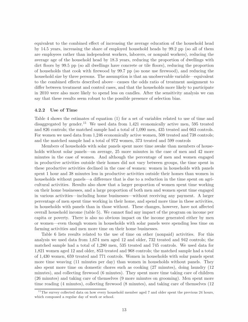
4.2.2 Use of Time

Table 4 shows the estimates of equation (1) for a set of variables related to use of time anddisaggregated by gender.11 We used data from 1,421 economically active men, 595 treatedand 826 controls; the matched sample had a total of 1,090 men, 435 treated and 663 controls.For women we used data from 1,246 economically active women, 508 treated and 738 controls;and the matched sample had a total of 972 women, 373 treated and 599 controls

Members of households with solar panels spent more time awake than members of house-holds without solar panels—on average, 25 more minutes in the case of men and 42 moreminutes in the case of women. And although the percentage of men and women engagedin productive activities outside their homes did not vary between groups, the time spent inthese productive activities declined in the case of women: women in households with panelsspent 1 hour and 38 minutes less in productive activities outside their homes than women inhouseholds without panels—a difference that is due to a reduction in the time spent on agri-cultural activities. Results also show that a larger proportion of women spent time workingon their home businesses, and a large proportion of both men and women spent time engagedin various activities—including home businesses—without receiving any payment. A largerpercentage of men spent time working in their home, and spend more time in these activities,in households with panels than in those without. These changes, however, have not affectedoverall household income (table 5). We cannot find any impact of the program on income percapita or poverty. There is also no obvious impact on the income generated either by menor women—even though women in households with solar panels were spending less time onfarming activities and men more time on their home businesses.

Table 6 lists results related to the use of time on other (nonpaid) activities. For thisanalysis we used data from 1,674 men aged 12 and older, 732 treated and 942 controls; thematched sample had a total of 1,280 men, 535 treated and 745 controls. We used data for1,821 women aged 12 and older, 853 treated and 968 controls; the matched sample had a totalof 1,430 women, 659 treated and 771 controls. Women in households with solar panels spentmore time weaving (11 minutes per day) than women in households without panels. Theyalso spent more time on domestic chores such as cooking (27 minutes), doing laundry (12minutes), and collecting firewood (6 minutes). They spent more time taking care of children(26 minutes) and taking care of themselves (9 more minutes on grooming). Men spent moretime reading (4 minutes), collecting firewood (8 minutes), and taking care of themselves (12

11The survey collected data on how every household member aged 7 and older spent the previous 24 hours,which composed a regular day of work or school.

13

Table 4: Use of Time: Productive Activities



Treated Controls S.E. hidden bias

Men that spent time...

Eating, sleeping, and resting (%) 1.000 0.999 0.001 0.001 0.86 (-) > 2

Eating, sleeping, and resting (minutes) 643.924 669.147 -25.223 8.362 -3.02*** (-) 1.2-1.3

In productive activities (%) 0.971 0.977 -0.006 0.012 -0.49 (-) > 2

In productive activities (minutes) 450.549 465.454 -14.905 14.528 -1.03 (-) > 2

In agricultural activities (%) 0.798 0.840 -0.042 0.032 -1.27 (-) 1.7-1.8

In agricultural activities (minutes) 291.327 318.592 -27.265 17.834 -1.53 (-) 1.3-1.4

In animal husbandry (%) 0.664 0.688 -0.024 0.037 -0.64 (-) 1.2-1.3

In animal husbandry (minutes) 102.579 107.990 -5.411 8.739 -0.62 (-) > 2

In their home business (%) 0.034 0.018 0.016 0.011 1.41 (-) 1.0-1.1

In their home business (minutes) 13.577 5.469 8.108 4.187 1.94* (-) > 2

Working w/o pay (%) 0.131 0.061 0.070 0.023 3.11*** (-) > 2

Working w/o pay (minutes) 28.540 15.380 13.160 6.299 2.09** (-) > 2

Women that spent time...

Eating, sleeping, and resting (%) 0.998 0.999 -0.001 0.002 -0.57 (-) > 2

Eating, sleeping, and resting (minutes) 642.071 684.440 -42.368 9.995 -4.24*** (-) 1.3-1.4

In productive activities (%) 0.947 0.964 -0.017 0.018 -0.99 (-) 1.5-1.6

In productive activities (minutes) 252.081 349.706 -97.625 16.089 -6.07*** (-) 1.5-1.6

In agricultural activities (%) 0.445 0.557 -0.112 0.045 -2.47** (-) 1.5-1.6

In agricultural activities (minutes) 88.576 150.424 -61.848 13.444 -4.60*** (-) 1.7-1.8

In animal husbandry (%) 0.881 0.877 0.004 0.029 0.13 (-) 1.1-1.2

In animal husbandry (minutes) 135.252 147.857 -12.604 9.582 -1.32 (-) > 2

In their home business (%) 0.056 0.027 0.029 0.017 1.71* (-) > 2

In their home business (minutes) 12.463 12.627 -0.164 5.680 -0.03 (-) > 2

Working w/o pay (%) 0.068 0.028 0.040 0.020 2.05** (-) > 2

Working w/o pay (minutes) 11.217 6.964 4.253 4.611 0.92 (-) > 2


Note: (†) t test for difference in means: *** denotes significance at 1%, ** significance at 5%, and * significanceat 10%. (‡) Odds ratio of treatment assignment: (+) denotes sensitivity analysis assuming overestimation oftreatment effect and (-) underestimation of treatment effect.

minutes). The increased time spent on collecting firewood indicates that households withsolar panels collected more firewood for free and consequently needed to buy less, savingsome money as shown previously.

Most of these results are robust to the possible presence of selection bias. But someare sensitive to possible deviations from the identifying unconfoundedness assumption—forexample, results related to the proportion of men that spent time on their home businesses orreading. In the first case, the magnitude of hidden bias that would undo the hypothesis testthat supports the result—Γ equal to 1.3 for the result becoming significant at 5 percent (andequal to 1.1 for becoming significant at 10 percent)—is equivalent to the effect of an additional7.6 years of schooling. The assumption is that the treatment effect on the proportion of menthat spent time on their home businesses is underestimated, and that households more likelyto participate in 2010 were also more likely to have men spending less time on their homebusinesses. In the second case, the magnitude of hidden bias that would undo the hypothesistest that supports the result—Γ equal to 1.1 for the result to become not significant at 5

14

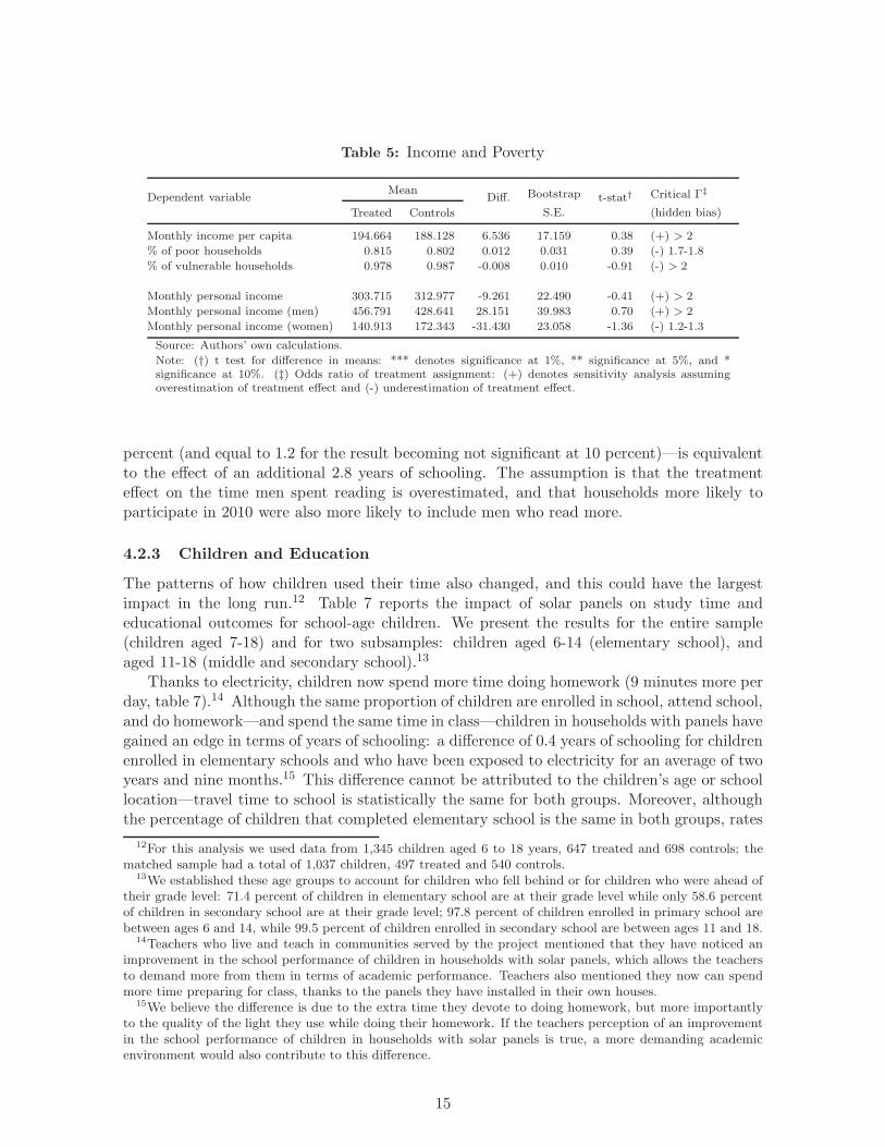
Table 5: Income and Poverty




Monthly income per capita 194.664 188.128 6.536 17.159 0.38 (+) > 2

% of poor households 0.815 0.802 0.012 0.031 0.39 (-) 1.7-1.8

% of vulnerable households 0.978 0.987 -0.008 0.010 -0.91 (-) > 2

Monthly personal income 303.715 312.977 -9.261 22.490 -0.41 (+) > 2

Monthly personal income (men) 456.791 428.641 28.151 39.983 0.70 (+) > 2

Monthly personal income (women) 140.913 172.343 -31.430 23.058 -1.36 (-) 1.2-1.3



percent (and equal to 1.2 for the result becoming not significant at 10 percent)—is equivalentto the effect of an additional 2.8 years of schooling. The assumption is that the treatmenteffect on the time men spent reading is overestimated, and that households more likely toparticipate in 2010 were also more likely to include men who read more.

4.2.3 Children and Education

The patterns of how children used their time also changed, and this could have the largestimpact in the long run.12 Table 7 reports the impact of solar panels on study time andeducational outcomes for school-age children. We present the results for the entire sample(children aged 7-18) and for two subsamples: children aged 6-14 (elementary school), andaged 11-18 (middle and secondary school).13

Thanks to electricity, children now spend more time doing homework (9 minutes more perday, table 7).14 Although the same proportion of children are enrolled in school, attend school,and do homework—and spend the same time in class—children in households with panels havegained an edge in terms of years of schooling: a difference of 0.4 years of schooling for childrenenrolled in elementary schools and who have been exposed to electricity for an average of twoyears and nine months.15 This difference cannot be attributed to the children’s age or schoollocation—travel time to school is statistically the same for both groups. Moreover, althoughthe percentage of children that completed elementary school is the same in both groups, rates

12For this analysis we used data from 1,345 children aged 6 to 18 years, 647 treated and 698 controls; thematched sample had a total of 1,037 children, 497 treated and 540 controls.

13We established these age groups to account for children who fell behind or for children who were ahead oftheir grade level: 71.4 percent of children in elementary school are at their grade level while only 58.6 percentof children in secondary school are at their grade level; 97.8 percent of children enrolled in primary school arebetween ages 6 and 14, while 99.5 percent of children enrolled in secondary school are between ages 11 and 18.

14Teachers who live and teach in communities served by the project mentioned that they have noticed animprovement in the school performance of children in households with solar panels, which allows the teachersto demand more from them in terms of academic performance. Teachers also mentioned they now can spendmore time preparing for class, thanks to the panels they have installed in their own houses.

15We believe the difference is due to the extra time they devote to doing homework, but more importantlyto the quality of the light they use while doing their homework. If the teachers perception of an improvementin the school performance of children in households with solar panels is true, a more demanding academicenvironment would also contribute to this difference.

15

Table 6: Use of time: Other Activities



Treated Controls S.E. hidden bias

Men that spent time...

Weaving (%) 0.007 0.009 -0.002 0.007 -0.27 (+) 1.4-1.5

Weaving (minutes) 0.511 1.320 -0.809 1.279 -0.63 (+) > 2

Reading (%) 0.220 0.171 0.049 0.029 1.72* (+) 1.2-1.3

Reading (minutes) 12.944 9.422 3.522 1.781 1.98** (+) 1.1-1.2

Taking care of children (%) 0.180 0.153 0.027 0.028 0.95 (+) 1.5-1.6

Taking care of children (minutes) 9.721 7.381 2.339 1.740 1.34 (+) > 2

Collecting firewood (%) 0.387 0.353 0.034 0.035 0.98 (+) 1.5-1.6

Collecting firewood (minutes) 32.794 24.624 8.171 3.604 2.27** (+) 1.1-1.2

Cooking (%) 0.062 0.071 -0.010 0.019 -0.51 (+) 1.5-1.6

Cooking (minutes) 7.934 7.127 0.807 2.446 0.33 (+) > 2

Doing laundry (%) 0.062 0.062 0.000 0.017 -0.03 (+) 1.2-1.3

Doing laundry (minutes) 4.391 3.481 0.910 1.235 0.74 (+) 1.1-1.2

On personal care (%) 0.978 0.956 0.022 0.012 1.75* (+) 1.2-1.3

On personal care (minutes) 42.896 31.197 11.699 2.020 5.79*** (+) 1.9-2.0

Women that spent time...

Weaving (%) 0.540 0.440 0.100 0.046 2.18** (+) 1.1-1.2

Weaving (minutes) 67.181 56.146 11.035 5.693 1.94* (+) 1.2-1.3

Reading (%) 0.125 0.122 0.003 0.025 0.12 (+) 1.7-1.8

Reading (minutes) 6.859 6.310 0.549 1.559 0.35 (+) > 2

Taking care of children (%) 0.756 0.663 0.094 0.033 2.83*** (+) 1.1-1.2

Taking care of children (minutes) 69.278 42.878 26.400 5.117 5.16*** (+) 1.4-1.5

Collecting firewood (%) 0.341 0.304 0.037 0.030 1.21 (+) 1.7-1.8

Collecting firewood (minutes) 24.440 18.410 6.030 2.571 2.34** (+) 1.3-1.4

Cooking (%) 0.786 0.693 0.093 0.031 2.98*** (+) 1.4-1.5

Cooking (minutes) 137.862 108.172 29.690 6.346 4.68*** (+) 1.3-1.4

Doing laundry (%) 0.435 0.339 0.096 0.036 2.69*** (+) 1.4-1.5

Doing laundry (minutes) 43.750 31.739 12.011 3.980 3.02*** (+) 1.2-1.3

On personal care (%) 0.961 0.959 0.002 0.014 0.18 (+) 1.6-1.7

On personal care (minutes) 43.289 34.634 8.655 1.965 4.41*** (+) 1.4-1.5



of enrollment in secondary school are larger for children with electricity.16 Because returnson education range between 7 to 11 percent, these differences, if they persist, can translateinto higher incomes in the future for children in households with electricity.17

It is important to point out that because only a small percentage of households use solarpanels to watch TV (5 percent of households)—and that because time spent watching TVmay reduce time spent studying, consequently affecting student performance—the externalvalidity of these findings is limited. These results might not be extrapolated to electrification

16The percentage of children who repeated a grade is statistically the same in both groups so the higherenrollment rate cannot be attributed to differences in grade retention.

17See Psacharopoulos and Patrinos (2002), and Duflo (2001).

16

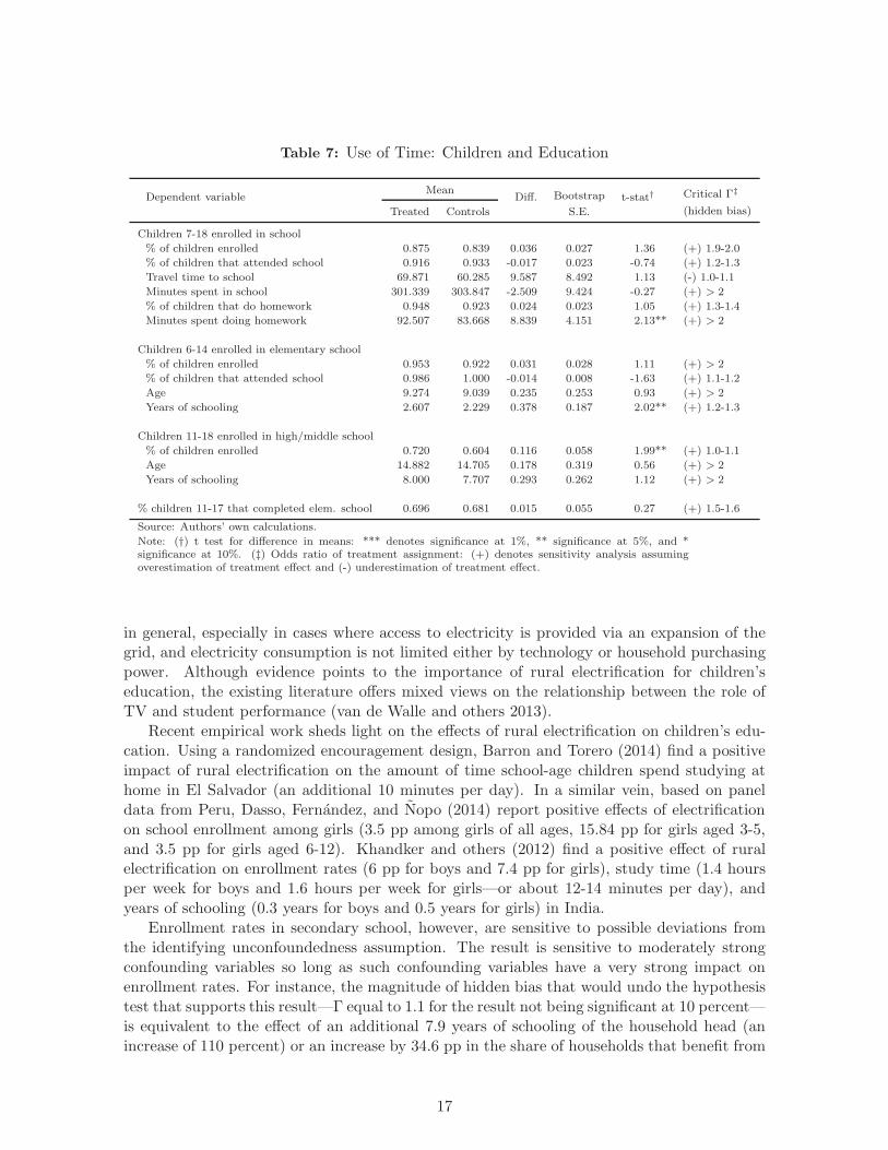
Table 7: Use of Time: Children and Education




Children 7-18 enrolled in school

% of children enrolled 0.875 0.839 0.036 0.027 1.36 (+) 1.9-2.0

% of children that attended school 0.916 0.933 -0.017 0.023 -0.74 (+) 1.2-1.3

Travel time to school 69.871 60.285 9.587 8.492 1.13 (-) 1.0-1.1

Minutes spent in school 301.339 303.847 -2.509 9.424 -0.27 (+) > 2

% of children that do homework 0.948 0.923 0.024 0.023 1.05 (+) 1.3-1.4

Minutes spent doing homework 92.507 83.668 8.839 4.151 2.13** (+) > 2

Children 6-14 enrolled in elementary school

% of children enrolled 0.953 0.922 0.031 0.028 1.11 (+) > 2

% of children that attended school 0.986 1.000 -0.014 0.008 -1.63 (+) 1.1-1.2

Age 9.274 9.039 0.235 0.253 0.93 (+) > 2

Years of schooling 2.607 2.229 0.378 0.187 2.02** (+) 1.2-1.3

Children 11-18 enrolled in high/middle school

% of children enrolled 0.720 0.604 0.116 0.058 1.99** (+) 1.0-1.1

Age 14.882 14.705 0.178 0.319 0.56 (+) > 2

Years of schooling 8.000 7.707 0.293 0.262 1.12 (+) > 2

% children 11-17 that completed elem. school 0.696 0.681 0.015 0.055 0.27 (+) 1.5-1.6



in general, especially in cases where access to electricity is provided via an expansion of thegrid, and electricity consumption is not limited either by technology or household purchasingpower. Although evidence points to the importance of rural electrification for children’seducation, the existing literature offers mixed views on the relationship between the role ofTV and student performance (van de Walle and others 2013).

Recent empirical work sheds light on the effects of rural electrification on children’s edu-cation. Using a randomized encouragement design, Barron and Torero (2014) find a positiveimpact of rural electrification on the amount of time school-age children spend studying athome in El Salvador (an additional 10 minutes per day). In a similar vein, based on paneldata from Peru, Dasso, Fernandez, and Nopo (2014) report positive effects of electrificationon school enrollment among girls (3.5 pp among girls of all ages, 15.84 pp for girls aged 3-5,and 3.5 pp for girls aged 6-12). Khandker and others (2012) find a positive effect of ruralelectrification on enrollment rates (6 pp for boys and 7.4 pp for girls), study time (1.4 hoursper week for boys and 1.6 hours per week for girls—or about 12-14 minutes per day), andyears of schooling (0.3 years for boys and 0.5 years for girls) in India.

Enrollment rates in secondary school, however, are sensitive to possible deviations fromthe identifying unconfoundedness assumption. The result is sensitive to moderately strongconfounding variables so long as such confounding variables have a very strong impact onenrollment rates. For instance, the magnitude of hidden bias that would undo the hypothesistest that supports this result—Γ equal to 1.1 for the result not being significant at 10 percent—is equivalent to the effect of an additional 7.9 years of schooling of the household head (anincrease of 110 percent) or an increase by 34.6 pp in the share of households that benefit from

17

the conditional cash-transfer program Juntos; the assumption is that the treatment effect onenrollment rates is overestimated and that households most likely to participate in 2010 werealso most likely to send their children to secondary school.18 It is important to point outthat the number of years of schooling of the household head (3.77)—and, specifically femalehousehold heads (2.76)—are statistically the same in the treatment and control groups, andthat there is no obvious reason to think that households most likely to participate in 2010were more likely to send their children to secondary school.

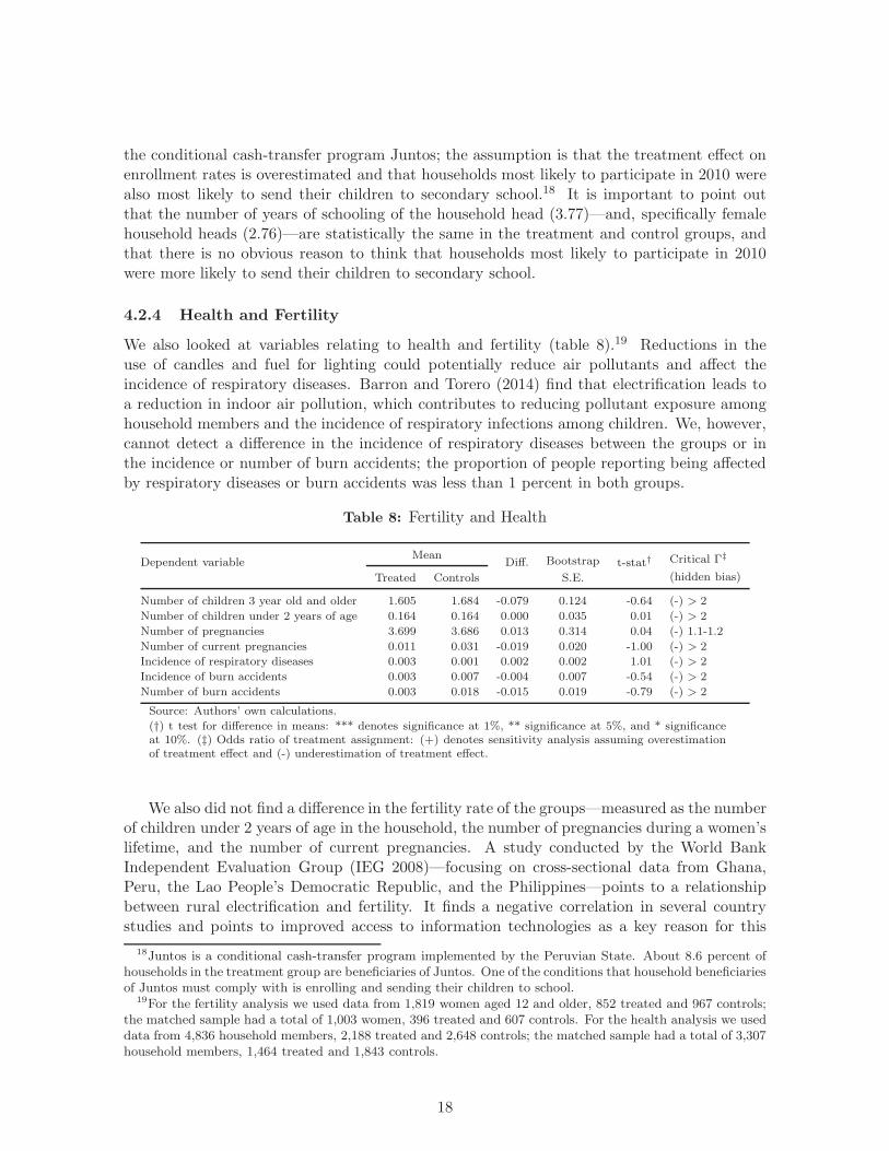
4.2.4 Health and Fertility

We also looked at variables relating to health and fertility (table 8).19 Reductions in theuse of candles and fuel for lighting could potentially reduce air pollutants and affect theincidence of respiratory diseases. Barron and Torero (2014) find that electrification leads toa reduction in indoor air pollution, which contributes to reducing pollutant exposure amonghousehold members and the incidence of respiratory infections among children. We, however,cannot detect a difference in the incidence of respiratory diseases between the groups or inthe incidence or number of burn accidents; the proportion of people reporting being affectedby respiratory diseases or burn accidents was less than 1 percent in both groups.

Table 8: Fertility and Health




Number of children 3 year old and older 1.605 1.684 -0.079 0.124 -0.64 (-) > 2

Number of children under 2 years of age 0.164 0.164 0.000 0.035 0.01 (-) > 2

Number of pregnancies 3.699 3.686 0.013 0.314 0.04 (-) 1.1-1.2

Number of current pregnancies 0.011 0.031 -0.019 0.020 -1.00 (-) > 2

Incidence of respiratory diseases 0.003 0.001 0.002 0.002 1.01 (-) > 2

Incidence of burn accidents 0.003 0.007 -0.004 0.007 -0.54 (-) > 2

Number of burn accidents 0.003 0.018 -0.015 0.019 -0.79 (-) > 2


(†) t test for difference in means: *** denotes significance at 1%, ** significance at 5%, and * significanceat 10%. (‡) Odds ratio of treatment assignment: (+) denotes sensitivity analysis assuming overestimationof treatment effect and (-) underestimation of treatment effect.

We also did not find a difference in the fertility rate of the groups—measured as the numberof children under 2 years of age in the household, the number of pregnancies during a women’slifetime, and the number of current pregnancies. A study conducted by the World BankIndependent Evaluation Group (IEG 2008)—focusing on cross-sectional data from Ghana,Peru, the Lao People’s Democratic Republic, and the Philippines—points to a relationshipbetween rural electrification and fertility. It finds a negative correlation in several countrystudies and points to improved access to information technologies as a key reason for this

18Juntos is a conditional cash-transfer program implemented by the Peruvian State. About 8.6 percent ofhouseholds in the treatment group are beneficiaries of Juntos. One of the conditions that household beneficiariesof Juntos must comply with is enrolling and sending their children to school.

19For the fertility analysis we used data from 1,819 women aged 12 and older, 852 treated and 967 controls;the matched sample had a total of 1,003 women, 396 treated and 607 controls. For the health analysis we useddata from 4,836 household members, 2,188 treated and 2,648 controls; the matched sample had a total of 3,307household members, 1,464 treated and 1,843 controls.

18

outcome. La Ferrara, Chong and Duryea (2008) provide evidence from Brazil supportingthe idea that television soap operas and the role models they offer have a negative effect onfertility. Jensen and Oster (2009) also highlight the impact of television on womens statusand fertility. Using data from India, they investigate the rollout of cable TV and find thatwomen’s fertility and acceptance of domestic violence (as reported by women themselves ininterviews) decreases with the introduction of cable TV at the village level. On a somewhatsimilar note, Peters and Vance (2011) find that electrification has opposite effects on fertilityin urban and rural areas, positive in the former and negative in the latter.

These results are robust to the possible presence of selection bias. The only result sensitiveto possible deviations from the identifying unconfoundedness assumption is the number ofpregnancies: the magnitude of hidden bias that would undo the hypothesis test that supportthis result—Γ equal to 1.2 for the result becoming significant at 5 percent—is equivalentto the effect of an additional 1.34 persons in the household. The assumption is that thetreatment effect on the number of pregnancies is underestimated, and that households morelikely to participate in 2010 were also more likely to include women who had undergone fewerpregnancies.

5 Conclusion and Policy Recommendations

This paper evaluates the impact of rural electrification on household well-being. Using afee-for-service model, AMP offers access to affordable electricity to low-income households—80.8 percent of its clients are poor—without jeopardizing the organizations financial viability.AMP’s fee-for-service model does not require large outlays of money. Any equipment thatneeds to be replaced, as well as system maintenance, is covered by the monthly fee thatthe client pays to AMP. Savings of what households would normally spend on traditionalsources of energy—candles and batteries for flashlights—allow these households to cover thesubsidized monthly fee for electricity.

AMP clients mainly use the electricity provided for lightning. Although they have theability to connect low-power consumption appliances, only a small percentage of beneficiariesuse the available energy to connect a radio or TV or to charge a mobile phone. Electric lighthas allowed households to lengthen the day: people spend more time awake, and women inparticular have changed how they use their time. Women in households with solar panelsspend less time in productive activities outside the household but more time in household-related activities such as taking care of children and cooking; a larger percentage also spendmore time on their home businesses.

The most important result is related to children’s study time. Children in households withpanels spend more time doing homework, and this has translated in an advantage in school: again of 0.4 years of schooling for children enrolled in elementary school who have been exposedto electricity for an average of two years and nine months. This difference cannot be attributedto children’s age—statistically the same—or the location and availability of schools: traveltime to school and enrollment is statistically the same for children in households with andwithout panels. Moreover, although the percentage of children who completed elementaryschool is the same in both groups, enrollment rates in secondary school are higher for childrenwith electricity. If these differences persist over time, it is expected that children in householdswith electricity will be able to generate higher incomes in the future.

These households’ economic benefits and welfare promise to improve further if the energy

19

provided by the panels is harnessed beyond its use for lighting (savings on batteries forradio, greater access to information through radio and TV, and so on). Understanding andaddressing the reasons why households are limiting the use of the panel to lighting mightincrease the benefits that electricity brings to these homes.

AMP seems to have achieved a balance between financial viability and a focus on low-income customers. Working in coordination with the Peruvian government, and having ob-tained the first rural electric concession based exclusively on solar PV systems, AMP hasreduced the likelihood of an unexpected power grid expansion that would eat into its cus-tomer base before it recoups its investment in equipment. This coordination reduces risk tothe fee-for-service model used by AMP and gives it financial viability. Because evidence sug-gests that the increase in coverage comes mainly from extensive growth of the network (intonew communities) rather than intensive growth (connecting unconnected homes in commu-nities that are already electrified), the fee-for-service model requires taking into account thenational expansion of the network to stay viable in the long term. In Peru the Ministry ofEnergy and Mines has developed a National Plan for Rural Electrification that identifies geo-graphic areas where PV systems are good candidates for domestic or communal use, whetherbecause it is inconvenient or impossible to connect them to large-scale power systems (as inthe case of dispersed households with low purchasing power and poor road infrastructure).Such government initiatives support the financial viability of AMP’s fee-for-service modelwithout compromising a focus on low-income populations.

20

References

[1] Aakvik, A. 2001. “Bounding a Matching Estimator: The Case of a Norwegian TrainingProgram.” Oxford Bulletin of Economics and Statistics 63(1): 115-43.

[2] Abadie, A., and G. Imbens. 2008. “On the Failure of the Bootstrap for Matching Esti-mators.” Econometrica, 76(6): 1537-57.

[3] Aguirre, J. 2014. “Impact of Rural Electrification on Education: A Case Study fromPeru.” Mimeo, Research Center, Universidad del Pacfico (Peru) and Department of Eco-nomics, Universidad de San Andres (Argentina).

[4] Barron, M., and M. Torero. 2014. “Short Term Effects on Household Electrification:Experimental Evidence from Northern El Salvador.” Mimeo.

[5] Becker, S., and M. Caliendo. 2007. “Sensitivity Analysis for Average Treatment Effects.”The Stata Journal 7(1): 71-83.

[6] Caliendo, M., and S. Kopening. 2008. “Some Practical Guidance for the Implementationof Propensity Score Matching.” Journal of Economic Surveys 22: 31-72.

[7] Chakravorty, U., M. Pelli, and B. Marchand. 2014. “Does the Quality of ElectricityMatter? Evidence from Rural India.” CESIfo Working Paper No. 4457.

[8] Dasso, R., F. Fernandez, and H. Nopo. 2014. “Electrification and Educational Outcomesin Rural Peru.” Mimeo, Inter-American Development Bank, Washington, DC.

[9] Dinkelman, T. 2011. “The Effects of Rural Electrication on Employment: New Evidencefrom South Africa.” American Economic Review 101(7): 3078108.

[10] DiPrete, T., and M. Gangl. 2004. “Assessing Bias in the Estimation of Causal Effects:Rosenbaum Bounds on Matching Estimators and Instrumental Variables Estimation withImperfect Instruments.” Sociological Methodology 34(1): 271-310.

[11] Duflo, E. 2001. “Schooling and Labor Market Consequences of School Construction inIndonesia: Evidence from an Unusual Policy Experiment.” American Economic Review

91(4): 795-813.

[12] Gonzalez, M., and M. Rossi. 2006. “The Impact of Electricity Sector Privatization onPublic Health.” IDB Working Paper No. 219, Inter-American Development Bank, Wash-ington, DC.

[13] Heinrich, C., A. Maffioli, and G. Vazquez. 2010. “A Primer for Applying Propensity-Score Matching.” SPD Working Papers 1005, Inter-American Development Bank, Officeof Strategic Planning and Development Effectiveness (SPD), Washington, DC.

[14] IEA (International Energy Agency). 2014. World Energy Investment Outlook. France:Organisation for Economic Co-operation and Development (OECD)/IEA.

[15] IEG (Independent Evaluation Group). 2008. The Welfare Impact of Rural Electrification:

A Reassessment of the Costs and Benefits. Washington, DC: World Bank.

21

[16] Jensen, R., and E. Oster. 2009. “The Power of TV: Cable Television and Womens Statusin India.” Quarterly Journal of Economics 124(3): 1057-94.

[17] Khandker, S., D. Barnes, and H. Samad. 2009. “Welfare Impacts of Rural Electrification.A Case Study from Bangladesh.” Policy Research Working Paper 4859, World Bank,Washington, DC.

[18] Khandker, S., D. Barnes, and H. Samad. 2013. “Welfare Impacts of Rural Electrification:A Panel Data Analysis from Vietnam.” Economic Development and Cultural Change

61(3): 659-92.

[19] Khandker, S., H. Samad, R. Ali, and D. Barnes. 2012. “Who Benefits Most from RuralElectrification? Evidence in India.” Policy Research Working Paper 6095, World Bank,Washington, DC.

[20] La Ferrara, E., A. Chong, and S. Duryea. 2008. “Soap Operas and Fertility: Evidencefrom Brazil.” IDB Working Paper No. 633, Inter-American Development Bank, Wash-ington, DC.

[21] Peters, J., and C. Vance. 2011. “Rural Electrification and Fertility: Evidence from Coted’Ivoire.” Journal of Development Studies 47 (5): 753-66.

[22] Psacharopoulos, G., and H. Patrinos. 2004. “Returns to Investment in Education: AFurther Update.” Education Economics 12(2): 111-34.

[23] Ravallion, M. 2008. “Evaluating Anti-Poverty Programs.” In Handbook of Development

Economics, Vol 4, eds. Schultz and Strauss, 3787-846. North-Holland: Amsterdam.

[24] Rosenbaum, P., and D. Rubin. 1983. “The Central Role of the Propensity Score inObservational Studies for Causal Effects.” Biometrika 70 (1): 41-55.

[25] Rud, J. 2012. “Electricity Provision and Industrial Development: Evidence from India.”Journal of Development Economics 97(2): 352-67.

[26] van de Walle, D., M. Ravallion, V. Mendiratta, and G. Koolwal. 2013. “Long-TermImpacts of Household Electrification in Rural India.” Policy Research Working PaperNo. 6527, World Bank, Washington, DC.

22

from candles to light - microsoft

Documents