fringe-follower regularized phase tracker for demodulation of closed-fringe interferograms

Servin et al. Vol. 18, No. 3 /March 2001/J. Opt. Soc. Am. A 689

Fringe-follower regularized phase tracker fordemodulation of closed-fringe interferograms

M. Servin

Centro de Investigaciones en Optica A. C., Apartado Postal 1-948, 37150 Leon, Guanajuato, Mexico

J. L. Marroquin

Centro de Investigacion en Matematicas A. C., Apartado Postal 402, 36000 Guanajuato, Guanajuato, Mexico

F. J. Cuevas

Centro de Investigaciones en Optica A. C., Apartado Postal 1-948, 37150 Leon, Guanajuato, Mexico

Received November 10, 1999; revised manuscript received September 22, 2000; accepted September 25, 2000

An algorithm for phase demodulation of a single interferogram that may contain closed fringes is presented.This algorithm uses the regularized phase-tracker system as a robust phase estimator, together with a newscanning technique that estimates the phase that initially follows the bright zones of the interferogram. Thecombination of these two elements constitutes a powerful new method, the fringe-follower regularized phasetracker, that makes it possible to correctly demodulate complex, single-image interferograms for which tradi-tional methods fail. © 2001 Optical Society of America

OCIS codes: 100.2650, 100.5070, 120.5050, 120.6150.

1. INTRODUCTIONThe main motivation for developing methods for estimat-ing the modulating phase of a single closed-fringe inter-ferogram is the difficulty (or impossibility) of obtainingphase shifted interferograms of transient events. Fringepatterns of transient events may be obtained by high-speed electronic speckle interferometry (ESPI) lightedwith a high-power twin-pulse laser. This double-pulseESPI technique yields a single fringe pattern, possibly in-cluding closed fringes. Even if static or harmonic analy-sis is done, the experimental setup required for phase-shifted interferograms to be obtained may beexperimentally difficult, as occurs, for example, when oneis analyzing the resonant harmonic modes of mechanicalparts.1

It is well known that the phase estimation of a singleclosed-fringe interferogram is one of the most difficultproblems to solve in interferometry. The main difficultystems from the inherent sign ambiguity that results whenone tries to recover the argument of a cosinusoidal func-tion: One may model an observed interferogram I(x, y)as

I~x, y ! 5 a~x, y ! 1 b~x, y !cos@f~x, y !#, (1)

where a(x, y) and b(x, y) are functions that model thebackground illumination variations and the local con-trast, respectively, and f(x, y) is the true phase field thatone tries to recover. It is clear that the observed imageI(x, y) will not change if one replaces f(x, y) with an-other phase function f1(x, y), given by

f1~x, y ! 5 H 2f~x, y ! 1 2kp ~x, y ! P S

f~x, y ! ~x, y ! ¹ S, (2)

0740-3232/2001/030689-07$15.00 ©

where S is an arbitrary set of pixels and k is an integer.When f is a nonmonotonically increasing function (thatgives rise to closed fringes) and the Hilbert transform isused as a demodulation method,2,3 one normally com-putes f1 instead of f for some unknown set S, introduc-ing spurious sign jumps into the solution. These meth-ods are based on the computation of the local phase of ananalytic function associated with the observed interfero-gram. This (complex-valued) analytic function is com-puted by taking the Fourier transform of the interfero-gram, filtering out a half-plane in the spatial frequencydomain, and taking the inverse Fourier transform of theresulting signal. In these cases the shape of the set S de-pends on which half-plane is filtered out by the methodand also on the particular form of the fringes. The cor-rection of the spurious phase-sign changes obtained bythe Fourier method may be difficult to determine, particu-larly for complex, noisy interferograms.4

The only way to determine that the two phases f andf1 are different is by phase shifting, because the follow-ing two fringe patterns are different:

cos@f~x, y ! 1 a# Þ cos@f1~x, y ! 1 a#. (3)

For this reason, the fringe pattern given by cos(f1 1 a)will have some high-frequency jumps along the boundaryof the region S that will be absent in cos(f 1 a) and thuswill clearly differentiate the two fringe patterns. On theother hand, the fringe pattern given by cos(f 1 a) willpreserve its frequency content.

The above remarks mean that phase demodulation of asingle fringe pattern is an ill-posed problem in a math-ematical sense (since it does not have a unique solutiongiven the observed data). Thus, to solve it, one must in-

2001 Optical Society of America

690 J. Opt. Soc. Am. A/Vol. 18, No. 3 /March 2001 Servin et al.

troduce prior constraints (e.g., that the recovered phasefield should be smooth) in the demodulation algorithm.This may be done, for example, by use of Bayesian esti-mation theory with prior Markov random field models;5,6

these methods, however, are computationally expensiveand not easy to implement.

Another way to introduce this prior smoothness con-straint is to require that f(x, y) be locally planar andpropagating an initial local phase estimate in a mannerreminiscent of the well-known phase-locked loop7,8 tech-nique that is widely used in telecommunications.8 Thisis the basis for the regularized phase-tracker (RPT)technique,9 which has the advantages of simplicity, com-putational efficiency, and the fact that it produces an es-timate of the unwrapped phase directly, making unwrap-ping (which sometimes may be difficult) unnecessary. Itsmain drawback is that it often fails in the case of complexinterferograms generated by phase fields that containmany critical points (maxima, minima and saddles). Inthis paper we show that this failure may be corrected byadopting a more sophisticated scanning strategy in thepropagation stage. The resulting algorithm is a simple,yet powerful, method that is capable of demodulatingcomplex single-image interferograms in a computation-ally efficient way.

The paper is organized as follows: In Section 2 we de-scribe the basis of the RPT technique; in Section 3 we in-troduce the new algorithm; in Section 4 we present ex-perimental results that illustrate its performance; andfinally, in Section 5 we draw some conclusions.

2. REGULARIZED PHASE TRACKERFor the reader’s convenience, in this section we review theessentials of the RPT technique.9 The standard math-ematical model for a fringe pattern can be written asgiven in Eq. (1). To phase demodulate the irradiancegiven in Eq. (1) by using the proposed phase-tracking al-gorithm, we need a preprocessing step to eliminatea(x, y) and to force the term b(x, y) to be close to 1 overthe entire interferogram. To eliminate a(x, y) we maysimply use a high-pass filter. We control the spatialvariations in b(x, y) by clipping the amplitude of thefringe pattern in the range (21, 1). The amount of clip-ping is just enough to ensure that the minima andmaxima of the fringes fall within the range (21, 1). Oncethis is done, one may use a soft low-pass filter just toround the clipped fringes that were outside the normaliz-ing range. With this preprocessing we may rewrite Eq.(1) as

I8~x, y ! ' cos@f~x, y !#. (4)

In the RPT technique9 one assumes that locally the in-tensity of the fringe pattern may be considered spatiallymonochromatic, so its irradiance may be modeled as asinusoidal function that is phase modulated by a planep( ). Specifically, the proposed cost function to be mini-mized by the estimated phase f0(x, y) at each site (x, y)is

U~x, y ! 5 (~e,h!e~Nx,yùP !

$@I8~e, h! 2 cos p~x, y, e, h!#2

1 b@f0~e, h! 2 p~x, y, e, h!#2m~e, h!%, (5)

where

p~x, y, e, h! 5 f0~x, y !

1 vx~x, y !~x 2 e! 1 vy~x, y !~ y 2 h!,

(6)

where P is the region inside the interferogram’s pupil andmay be seen as a two-dimensional lattice that has validfringe data inside it (good amplitude modulation); Nx,y isa neighborhood region about the coordinate (x, y) wherethe phase is being estimated; and m(x, y) is an indicatorfield that equals 1 if the site (x, y) has already been phaseestimated and equals 0 otherwise. The functionsvx(x, y) and vy(x, y) are the estimated local frequenciesalong the x and y directions, respectively. These func-tions also represent the slopes in the x and y directions atsite (x, y) of the locally fitted phase plane. Finally, theparameter b is a constant regularizing parameter thatcontrols (along with the size of Nx,y) the smoothness ofthe detected phase f0(x, y).

The first term in Eq. (5) attempts to keep the localfringe model close to the observed irradiance in a least-squares sense within the neighborhood Nx,y . The secondterm enforces the assumption of smoothness and continu-ity, using only previously detected pixels f0(x, y) markedby m(x, y). To demodulate a given fringe pattern weneed to find the minimum of the cost function U(x, y) ateach site (x, y) with respect to the variables f0(x, y),vx(x, y), and vy(x, y).

Unfortunately the cost function U(x, y) in Eq. (5) isnonconvex, so fast optimizing techniques are precluded.Therefore we normally use fixed-step gradient descent tofind the optimum values for the needed variables. Thatis, given r (x, y) 5 ( f0 , vx , vy)T, we estimate the phaseand frequency at each site (x, y) according to

r k11~x, y ! 5 r k~x, y ! 2 m¹rU~x, y !, (7)

where m is the constant step of descent of the gradientsearch and ¹r is the gradient of U(x, y) with reference tothe three components of r (x, y) 5 ( f0 , vx , vy)T; that is,

¹rU~x, y ! 5 F ]U~x, y !

]f0~x, y !,

]U~x, y !

]vx~x, y !,

]U~x, y !

]vy~x, y !G . (8)

The constant phase step m for the f0(x, y) component inEq. (7) may be multiplied by 10 to accelerate the conver-gence rate. The gradient search method also needs astarting condition for r0 in Eq. (7). To demodulate theinitial pixel (seed pixel) at (x0 , y0) inside P, we have cho-sen as the initial condition the vector r0(x0 , y0)5 (0, 0, 0)T. When the seed vector r0(x0 , y0) is opti-mized by use of Eqs. (5)–(7) the regularizing term in Eq.(5) is not taken into account, given that the seed pixel isthe first one that is demodulated and that as a conse-quence the indicator function m(x, y) equals 0 all over thepupil P. Once the seed vector r(x0 , y0) is estimated[from expressions (4)–(6)], we may proceed with the restof the sites in P. The RPT system must follow a continu-


ous sequential path starting at the seed position, propa-gating the final condition of r (x0 , y0) in Eq. (7) as the ini-tial condition for the following adjacent site. So now theRPT technique proceeds from pixel to pixel until thewhole interferogram is phase demodulated.

The phase tracker as stated in Eqs. (5)–(7) may be usedto demodulate low-noise closed-fringe interferograms.However, in dealing with higher-noise closed-fringe inter-ferograms we must add another term into the cost func-tion U(x, y). This term is related to the fact that aslightly phase-shifted interferogram must also look simi-lar to the unshifted interferogram when we are lookingfor the smoothest phase that is compatible with the obser-vations I8( • ). Following this reasoning, Eq. (5) will bemodified as

U~x, y ! 5 (~e,h!e~Nx,yùS !

$@I8~e, h!

2 cos p~x, y, e, h!#2 1 @I8~e, h!

2 cos p1~x, y, e, h!#2 1 b@f0~e, h!

2 p~x, y, e, h!#2m~e, h!%, (9)

p1~x, y, e, h! 5 p~x, y, e, h! 1 a, (10)

where p(x, y, e, h) is given by Eq. (6). We recommendusing as constant phase shift a a value between a5 0.1p and a 5 0.3p rad. As we can see, p(•) and p1(•)differ only in the shift constant a, which means that theinterferogram’s irradiance I8(•) must appear to be some-where intermediate between cos( p) and cos( p1 a) in a least squares sense. As mentioned above, thisfact forces the RPT to look for the smoothest modulatingphase. Without this phase-shifted term a the phasetracker may easily fall into a spurious minimum when weare dealing with noisy closed-fringe interferograms. Thisfact also implies that the estimated phase will have somedistortion that may be removed afterward, as we will see.

It must be remarked that Eq. (9) is minimized whenthe RPT is scanning the interferogram for the first time toobtain the first phase estimation over the entire interfero-gram. After that, if a better phase estimation is desired,the sites may be visited once again in any desired order,provided that all of them are updated at least once. Dur-ing these additional iterations we must now minimize Eq.(5) [instead of Eq. (9)] because we no longer need the con-stant phase shift a that helped to discriminate thesmoothest modulating phase from among several closelycompeting solutions. In other words, the fact that oneminimizes Eq. (9) instead of Eq. (5) usually yields aslightly distorted demodulated phase. That is why it isoften necessary to perform additional minimization itera-tions on Eq. (5) to get closer to the undistorted estimatedphase.

3. FRINGE-FOLLOWER REGULARIZEDPHASE TRACKERIntuitively, the RPT works by finding a plane that bestfits both the local phase of the interferogram and the val-ues of the phase in a neighborhood that have already beenestimated. In addition to this, the estimated phase and

frequency serve as starting point for the next pixel to bedemodulated. With these facts in mind, it may be arguedthat the RPT has some inertia, which means that a com-plete specification for the RPT must include the two-dimensional scanning strategy, which defines the se-quence of pixels in the interferograms that must befollowed to demodulate it. In its original form,9 a de-modulating scanning sequence independent of the form ofthe fringe pattern was used. In complex fringe patterns,using this sequence caused the RPT’s inertia to inducethe RPT to take the wrong phase branch [i.e., f1 in Eq.(2)] when the system passed through stationary points,particularly saddle points.

The new algorithm presented here is based on a well-defined scanning strategy that depends on the form of theparticular fringe pattern. This new algorithm guaran-tees that the RPT will leave those difficult points wherethe system nay go wrong to be demodulated after theirsurrounding pixels are phase estimated. To this end, oneuses a scanning strategy that first scans the bright partsof the interferogram fringes.

Thus the fringe-pattern irradiance is used in this newalgorithm to guide the RPT. That is, the next pixel to beestimated is chosen as the one of maximum intensityamong the neighbors of the current pixel. Nevertheless,if the fringe pattern is too noisy, one should first pass itthrough a low-pass filter to obtain a smoother fringe pat-tern. This step is required because otherwise, the scan-ning sequence might look like a random walk instead ofpreferentially following the fringe brighter zones. Be-sides, the fact that one uses a binary pattern to guide thescanning sequence, simplifies the algorithm (see below)and produces better results, since the binary pattern pro-vides more support to the fitted planes. Thus we definethe following two-level fringe pattern

Ib~x, y ! 5 Thresh@I8~x, y ! ** LPF~x, y !#, (11)

where LPF is a low-pass convolution matrix, ** repre-sents the two-dimensional convolution, I(x, y) is the in-terferogram’s irradiance [Eq. (1)], and the operatorThresh( • ) is the binarizing operator.

The proposed fringe-follower RPT (FFRPT) (based onRef. 10) applied to the demodulation of a single interfero-gram may be outlined as follows:

1. Compute the histogram from the binary intensity ofIb(x, y) [Eq. (11)] and allocate memory for a first-in, first-out pixel register with every occurrence of the two valuesof Ib(x, y).

2. Select as seed or starting site any pixel situatedover a bright fringe in a region of highest signal-to-noiseratio and medium frequency content. Demodulate theseed pixel, optimizing for r using Eqs. (7)–(9).

3. Demodulate all eight adjacent sites around the seedpixel (to demodulate these sites, take as initial conditionthe already estimated phase and frequency of the seedsite) and enter them into the pixel registers according totheir intensity values in Ib(x, y).

4. Take the first pixel entered from the highest non-empty register, estimate all its eight connected neighbor-hood sites, and enter them into their corresponding regis-ters.


5. Repeat step 4 until all registers are empty.

After steps 1–5, all the sites in P will be phase and fre-quency estimated. This constitutes the first global esti-mation. An intuitive way of considering the first phaseestimation just presented is as a crystal-growing process,in which new molecules (phase-plane parameters) areadded to the bulk in that particular orientation (phaseand frequency) that minimizes the local crystal energy,given the geometric orientation of the previously posi-tioned molecules.

As mentioned, quite often one may improve the phaseestimate even further [because Eq. (9) was optimized in-stead of Eq. (5)] by applying one or several times the RPT[optimizing Eq. (4)] to the phase obtained during the firstcrystal-growing iteration [note that m(x, y) is now equalto 1 everywhere in P]. Given that we now have an initialphase and frequency estimate all over P, the followingphase-estimation improvements do not need to follow anyintelligent scanning sequence. All sites in P may be vis-ited in any desired order, provided that all the sites arevisited at least once. Another important remark con-cerning the additional optimizing of U(x, y) is that everytime a site (x, y) in P is visited, we must obtain the initialcondition for Eq. (5) from the previously estimated r(x, y)at that site and not from a neighboring site. Normallyone needs to make approximately five additional passes toobtain a good minimum of U(x, y) in Eq. (5) at every sitein P.

4. COMPUTER SIMULATION ANDEXPERIMENTAL RESULTSTo compare the new sequential strategy against what wasproposed in Ref. 9 and the technique proposed by Kreis,3

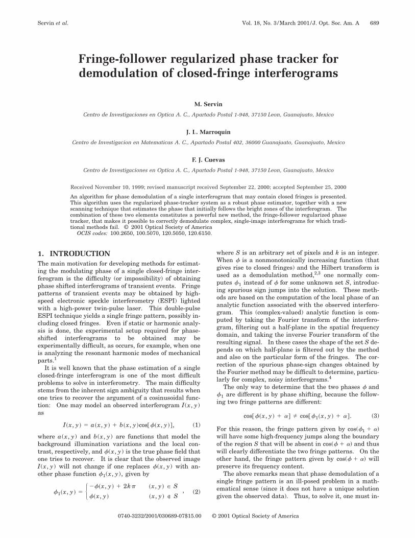
we carried out two computer simulations.In Fig. 1(a) we show a computer-generated speckle-

gram that has five stationary phase points and ;10p radof phase dynamic range. Figure 1(b) shows the phase ofthe complex analytical signal associated with the fringepattern given in Fig. 1(a). We may see that this phasemap is monotonically increasing in the y direction. Toobtain the expected hills and valleys on the true phase weneed to change the sign of the phase map in several re-gions before unwrapping it. This task is difficult to per-form by hand even when one has an expert eye; to achieve

Fig. 1. Computer-generated subtraction specklegram. (a)Fringe pattern being phase demodulated, (b) demodulated phasemap obtained by the Fourier method.

this task in a fully automatic way has proved to be a for-midable task even in noiseless computer-generated phasemaps that have few fringes and a single stationarypoint.2,3

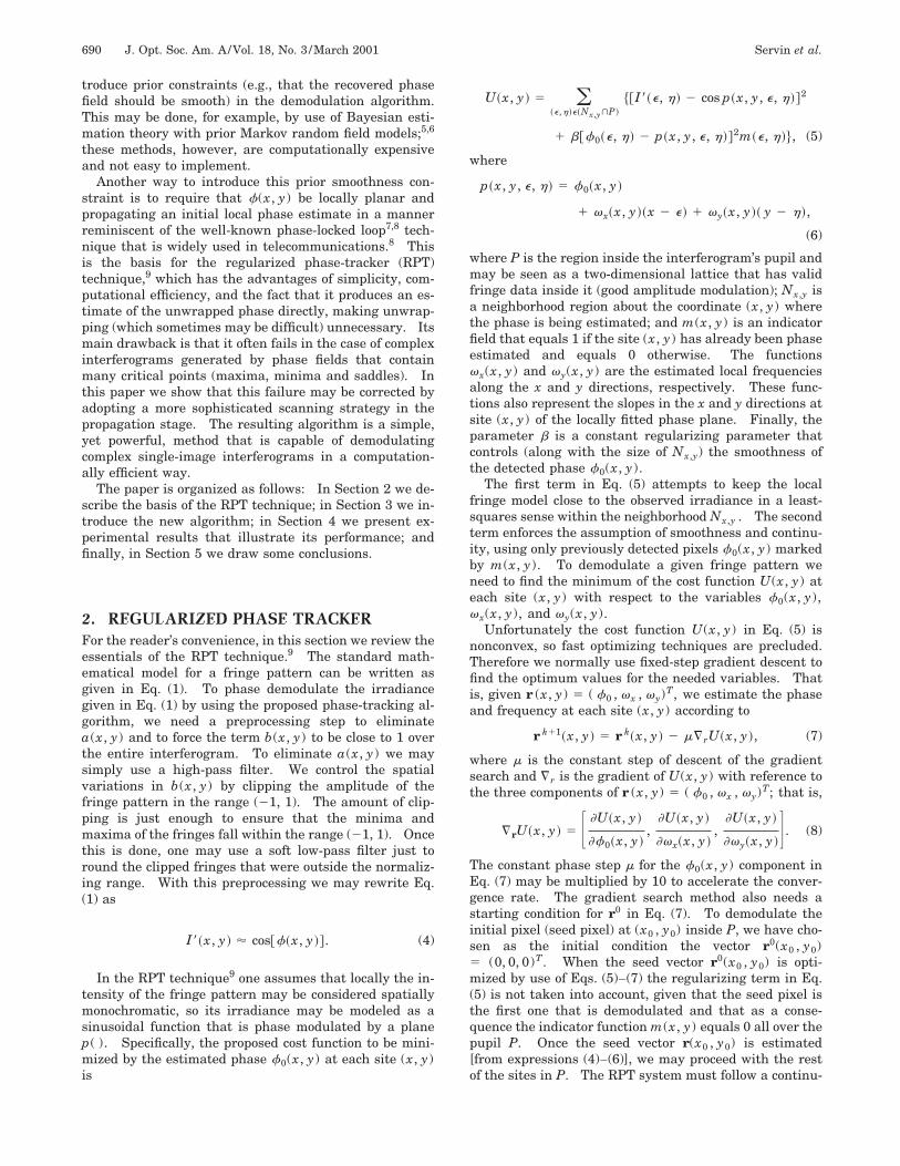
Figure 2(a) shows the same specklegram as in Fig. 1(a).Now we present an attempt to demodulate it by using theclassical RPT. Figures 1(b) and 1(c) show the evolutionof the flood-fill area being processed. We can see that thestrategy was simply an isotropic floodfill starting at thecenter of the interferogram. Figure 2(d) shows the re-sulting erroneous phase.

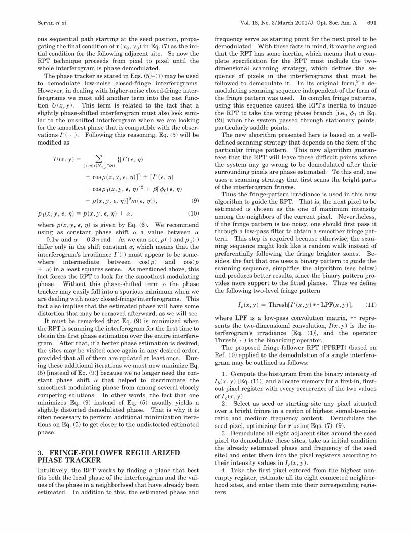
In contrast, in Fig. 3 we show this specklegram success-fully demodulated by the FFRPT. As we can see fromFig. 3(a), the noise in the fringe pattern is high. Figure3(b) shows the binarized interferogram. As mentioned,the FFRPT system preferentially follows the brighter in-tensity paths in the fringe pattern. In Fig. 3(c) we canshow the demodulating path followed by the algorithm.Proceeding with our demodulating sequence [Fig. 3(d)],we can see that the fringes around the phase extrema aredemodulated on a fringe-by-fringe basis. The last scan-ning state, seen in Fig. 3(e), shows how the smallest andmost difficult closed fringes are usually demodulated last.Finally, the demodulated phase is shown in Fig. 3(f). Asmentioned above, the FFRPT gives the demodulatedphase already unwrapped, but in Fig. 3(f) we have re-wrapped it for comparison with the fringe pattern [seeFig. 3(a)]. The main difficulty with the FFRPT resides inthe regions around which the phase has a saddle point.In Fig. 3(a) we have four such regions, as can be seen fromthe recovered phase [Fig. 3(f)]. As we can see from Figs.3(e) and 3(f), those regions were successfully demodulatedbecause the saddle points were demodulated only after

Fig. 2. Computer-generated subtraction specklegram. (a)Fringe pattern being phase demodulated; (b), (c) isotropic de-modulation path followed by the RPT; (d) wrongly demodulatedphase.


their surrounding sites were estimated. This fact is il-lustrated in Figs. 3(d) and 3(e). The reason why thesesaddle points were demodulated last is that the saddlepoints in this interferogram have a lower intensity thantheir neighboring pixels. If one has bright fringe data inthe saddle point of an interferogram, we recommend thatthe negative (with reversed contrast) of the fringe patternbe obtained first. In this way the region around thesaddle point will be dark, so it will be demodulated afterthe phase estimation of its neighboring sites. Here wehave used a 7 3 7 neighborhood Nx,y and phase shift a5 1.0 rad in Eq. (10). Four additional iterations withEq. (5) were used to reduce the phase distortion intro-duced by the use of a phase shift of a 5 1.0 rad in Eq. (9).

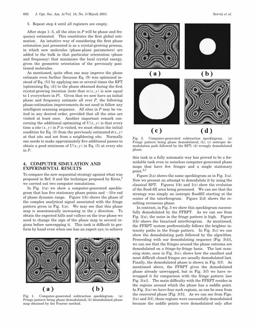
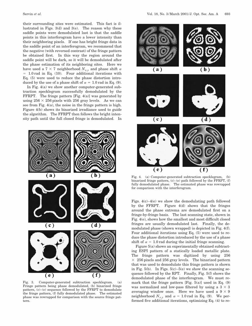
In Fig. 4(a) we show another computer-generated sub-traction specklegram successfully demodulated by theFFRPT. The fringe pattern [Fig. 4(a)] was generated byusing 256 3 256 pixels with 256 gray levels. As we cansee from Fig. 4(a), the noise in the fringe pattern is high.Figure 4(b) shows its binarized irradiance used to guidethe algorithm. The FFRPT then follows the bright inten-sity path until the full closed fringe is demodulated. In

Fig. 3. Computer-generated subtraction specklegram. (a)Fringe pattern being phase demodulated, (b) binarized fringepattern, (c)–(e) sequence followed by the FFRPT to demodulatethe fringe pattern, (f) fully demodulated phase. The estimatedphase was rewrapped for comparison with the source fringe pat-tern.

Figs. 4(c)–4(e) we show the demodulating path followedby the FFRPT. Figure 4(d) shows that the fringesaround the phase extrema are demodulated first on afringe-by-fringe basis. The last scanning state, shown inFig. 4(e), shows how the smallest and most difficult closedfringes are usually demodulated last. Finally, the de-modulated phase (shown wrapped) is depicted in Fig. 4(f).Four additional iterations using Eq. (5) were used to re-duce the phase distortion introduced by the use of a phaseshift of a 5 1.0 rad during the initial fringe scanning.

Figure 5(a) shows an experimentally obtained subtract-ing ESPI pattern of a statically loaded metallic plate.The fringe pattern was digitized by using 2563 256 pixels and 256 gray levels. The binarized patternthat was used to demodulate this fringe pattern is shownin Fig. 5(b). In Figs. 5(c)–5(e) we show the scanning se-quence followed by the RPT. Finally, Fig. 5(f) shows thedemodulated phase of the interferogram. We must re-mark that the fringe pattern [Fig. 5(a)] used in Eq. (9)was normalized and low-pass filtered by using a 3 3 3averaging window once. Here we have used a 9 3 9neighborhood Nx,y and a 5 1.0 rad in Eq. (9). We per-formed five additional iterations, optimizing Eq. (4) to re-

Fig. 4. (a) Computer-generated subtraction specklegram, (b)binarized fringe pattern, (c)–(e) path followed by the FFRPT, (f)fully demodulated phase. The estimated phase was rewrappedfor comparison with the interferogram.


duce the phase distortion introduced by using a phaseshift of a 5 1.0 rad in Eq. (9).

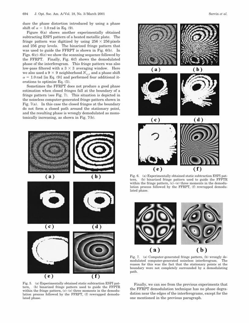
Figure 6(a) shows another experimentally obtainedsubtracting ESPI pattern of a heated metallic plate. Thefringe pattern was digitized by using 256 3 256 pixelsand 256 gray levels. The binarized fringe pattern thatwas used to guide the FFRPT is shown in Fig. 6(b). InFigs. 6(c)–6(e) we show the scanning sequence followed bythe FFRPT. Finally, Fig. 6(f) shows the demodulatedphase of the interferogram. This fringe pattern was alsolow-pass filtered with a 3 3 3 averaging window. Herewe also used a 9 3 9 neighborhood Nx,y and a phase shifta 5 1.0 rad [in Eq. (9)] and performed four additional it-erations to optimize Eq. (5).

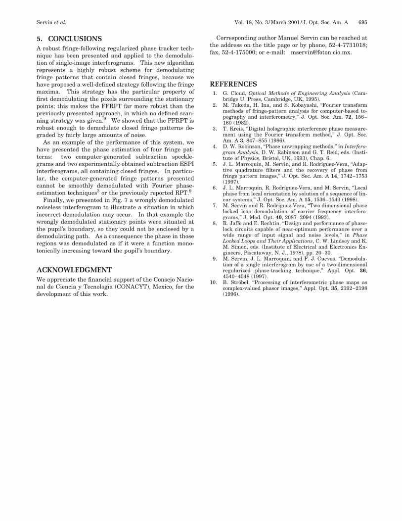
Sometimes the FFRPT does not produce a good phaseestimation when closed fringes fall at the boundary of afringe pattern (see Fig. 7). This situation is depicted inthe noiseless computer-generated fringe pattern shown inFig. 7(a). In this case the closed fringes at the boundarydo not form a closed path around the stationary point,and the resulting phase is wrongly demodulated as mono-tonically increasing, as shown in Fig. 7(b).

Fig. 5. (a) Experimentally obtained static subtraction ESPI pat-tern, (b) binarized fringe pattern used to guide the FFPTRwithin the fringe pattern, (c)–(e) three moments in the demodu-lation process followed by the FFRPT, (f) rewrapped demodu-lated phase.

Finally, we can see from the previous experiments thatthe FFRPT demodulation technique has no phase degra-dation near the edges of the interferograms, except for theone mentioned in the previous paragraph.

Fig. 6. (a) Experimentally obtained static subtraction ESPI pat-tern, (b) binarized fringe pattern used to guide the FFPTRwithin the fringe pattern, (c)–(e) three moments in the demodu-lation process followed by the FFRPT, (f) rewrapped demodu-lated phase.

Fig. 7. (a) Computer-generated fringe pattern, (b) wrongly de-modulated computer-generated noiseless interferogram. Thereason for this was the fact that the stationary points at theboundary were not completely surrounded by a demodulatingpath.


5. CONCLUSIONSA robust fringe-following regularized phase tracker tech-nique has been presented and applied to the demodula-tion of single-image interferograms. This new algorithmrepresents a highly robust scheme for demodulatingfringe patterns that contain closed fringes, because wehave proposed a well-defined strategy following the fringemaxima. This strategy has the particular property offirst demodulating the pixels surrounding the stationarypoints; this makes the FFRPT far more robust than thepreviously presented approach, in which no defined scan-ning strategy was given.9 We showed that the FFRPT isrobust enough to demodulate closed fringe patterns de-graded by fairly large amounts of noise.

As an example of the performance of this system, wehave presented the phase estimation of four fringe pat-terns: two computer-generated subtraction speckle-grams and two experimentally obtained subtraction ESPIinterferograms, all containing closed fringes. In particu-lar, the computer-generated fringe patterns presentedcannot be smoothly demodulated with Fourier phase-estimation techniques3 or the previously reported RPT.9

Finally, we presented in Fig. 7 a wrongly demodulatednoiseless interferogram to illustrate a situation in whichincorrect demodulation may occur. In that example thewrongly demodulated stationary points were situated atthe pupil’s boundary, so they could not be enclosed by ademodulating path. As a consequence the phase in thoseregions was demodulated as if it were a function mono-tonically increasing toward the pupil’s boundary.

ACKNOWLEDGMENTWe appreciate the financial support of the Consejo Nacio-nal de Ciencia y Tecnologıa (CONACYT), Mexico, for thedevelopment of this work.

Corresponding author Manuel Servin can be reached atthe address on the title page or by phone, 52-4-7731018;fax, 52-4-175000; or e-mail: [email protected].

REFERENCES1. G. Cloud, Optical Methods of Engineering Analysis (Cam-

bridge U. Press, Cambridge, UK, 1995).2. M. Takeda, H. Ina, and S. Kobayashi, ‘‘Fourier transform

methods of fringe-pattern analysis for computer-based to-pography and interferometry,’’ J. Opt. Soc. Am. 72, 156–160 (1982).

3. T. Kreis, ‘‘Digital holographic interference phase measure-ment using the Fourier transform method,’’ J. Opt. Soc.Am. A 3, 847–855 (1986).

4. D. W. Robinson, ‘‘Phase unwrapping methods,’’ in Interfero-gram Analysis, D. W. Rabinson and G. T. Reid, eds. (Insti-tute of Physics, Bristol, UK, 1993), Chap. 6.

5. J. L. Marroquin, M. Servin, and R. Rodriguez-Vera, ‘‘Adap-tive quadrature filters and the recovery of phase fromfringe pattern images,’’ J. Opt. Soc. Am. A 14, 1742–1753(1997).

6. J. L. Marroquin, R. Rodriguez-Vera, and M. Servin, ‘‘Localphase from local orientation by solution of a sequence of lin-ear systems,’’ J. Opt. Soc. Am. A 15, 1536–1543 (1998).

7. M. Servin and R. Rodriguez-Vera, ‘‘Two dimensional phaselocked loop demodulation of carrier frequency interfero-grams,’’ J. Mod. Opt. 40, 2087–2094 (1993).

8. R. Jaffe and E. Rechtin, ‘‘Design and performance of phase-lock circuits capable of near-optimum performance over awide range of input signal and noise levels,’’ in PhaseLocked Loops and Their Applications, C. W. Lindsey and K.M. Simon, eds. (Institute of Electrical and Electronics En-gineers, Piscataway, N. J., 1978), pp. 20–30.

9. M. Servin, J. L. Marroquin, and F. J. Cuevas, ‘‘Demodula-tion of a single interferogram by use of a two-dimensionalregularized phase-tracking technique,’’ Appl. Opt. 36,4540–4548 (1997).

10. B. Strobel, ‘‘Processing of interferometric phase maps ascomplex-valued phasor images,’’ Appl. Opt. 35, 2192–2198(1996).

fringe-follower regularized phase tracker for demodulation of closed-fringe interferograms

Documents