frequency domain analysis of dynamic systemsgeromel/rob_transf.pdf · chapter ii - laplace and z...

CHAPTER II - Laplace and Z transforms

FREQUENCY DOMAIN ANALYSIS OF

DYNAMIC SYSTEMS

JOSE C. GEROMEL

DSCE / School of Electrical and Computer EngineeringUNICAMP, CP 6101, 13083 - 970, Campinas, SP, Brazil,

[email protected]

Campinas, Brazil, August 2006

1 / 52


Contents

1 CHAPTER II - Laplace and Z transformsLaplace transformDefinition and domain determinationTime invariant systemsTime varying systemsNonrational transformsZ transformDefinition and domain determinationTime invariant systemsTime varying systemsProblems

2 / 52


Laplace transform

Laplace transform

The Laplace transform of the function f (t) : R → C denotedas f (s) or L(f ) is a function of complex variable

f (s) : D(f ) → C

where D(f ) is its domain and

f (s) =

∫ ∞

−∞

f (t)e−stdt (1)

D(f ) := {s ∈ C : f (s) exists } (2)

It is important to keep in mind that f (s) exists means that theintegral in (1) converges and is finite.

3 / 52


Laplace transform

Laplace transform

Generally D(f ) is a strict subset of C. In this case, there

exists s ∈ C such that s /∈ D(f ) and hence, the determination

of the domain D(f ) is an essential issue when dealing withLaplace transform.

Important : The domain of the Laplace transform D(f )strongly depends on the domain of the function f (t). As it willbe clear in the sequel :

t ∈ [0,+∞) =⇒ Re(s) ∈ (α,∞)

t ∈ (−∞, 0] =⇒ Re(s) ∈ (−∞, β)

t ∈ (−∞,∞) =⇒ Re(s) ∈ (α, β)

for some α, β ∈ R.

4 / 52


Laplace transform

Laplace transform

For each function the Laplace transform (if any) is given :

f (t) = e−at : R → C and D(f ) = ∅.f (t) = e−at : [0,+∞) → C and

f (s) =1

s + a, D(f ) = {s ∈ C : Re(s) > −Re(a)}

f (t) = e−at : (−∞, 0] → C and

f (s) = − 1

s + a, D(f ) = {s ∈ C : Re(s) < −Re(a)}

f (t) = e−a|t| : (−∞,+∞) → C and

f (s) = − 2a

s2 − a2, D(f ) = {s ∈ C : |Re(s)| < Re(a)}

5 / 52


Definition and domain determination


The exponential function e−λt : R → C for any λ ∈ C doesnot admit a Laplace transform. Hence, for functions withdomain t ∈ R the Laplace transform is too restrictive, beinguseless for solving linear differential equations. To circumventthis difficulty, let us restrict our interest to functions definedfor t ∈ [0,+∞), in which case we have

f (s) :=

∫ ∞

0f (t)e−stdt

with domain of the general form

D(f ) := {s ∈ C : Re(s) > α}

for some α ∈ R to be adequately determined.

6 / 52




Important class : There exists sf ∈ C such that the limit

limτ→∞

∫ τ

0|f (t)e−sf t |dt

exists and is finite.

Lemma (Domain characterization)

For the functions of this class the following hold :

Any s ∈ C satisfying Re(s) ≥ Re(sf ) belongs to D(f ).

There exists M finite such that |f (s)| ≤ M for all s ∈ D(f ).

7 / 52




General form : Functions defined for all t ≥ 0 :

D(f ) := {s ∈ C : Re(s) > α}

Domain determination : Given a function f (t), determine theminimum value of α ∈ R such that

limτ→∞

∫τ

0

|f (t)e−αt |dt < ∞

Domain determination : Given a function f (s), determine theminimum value of α ∈ R such that f (s) remains analytic in allpoints of the complex plane belonging to D(f ).

8 / 52




The function f (s) = e−s

sis not analytic at s = 0. Its Laurent

series is

f (s) =1

s− 1 +

s

2− s2

6+ · · ·

consequently

D(f ) := {s ∈ C : Re(s) > 0}

The function f (s) = 1−e−s

sis analytic at s = 0. Its Taylor

series is

f (s) = 1− s

2+

s2

6− · · ·

consequently

D(f ) := {s ∈ C : Re(s) > −∞} = C

9 / 52




Rational function :

f (s) :=N(s)

D(s)=

∑mi=0 bis

i

∑ni=0 ais

i

where m ≤ n, bi ∈ R for all i = 1, · · · ,m and ai ∈ R for alli = 1, · · · , n. If m = n it is called proper otherwise strictlyproper. It is not analytic at the poles pi , i = 1, · · · , n roots ofD(s) = 0. Hence

α = maxi=1,··· ,n

Re(pi )

Unitary (Dirac) impulse :

δ(s) = 1 , D(δ) = C

10 / 52




Several calculations involving Laplace transform depend onthe precise determination of its domain :

Integral : The integral of a function f (t) defined for all t ≥ 0can be determined from

∫ ∞

0

f (t)dt = f (0)

whenever 0 ∈ D(f ).Limit : The limit of a function f (t) defined for all t ≥ 0 can bedetermined from

limt→∞

f (t) = lims→0

sf (s)

whenever 0 ∈ D(sf ).

11 / 52



Properties

Basic properties for dynamic systems analysis, valid forfunctions defined in the time domain t ≥ 0 and scalarsθ1, θ2, · · · .

Linearity :

L(∑

i

θi fi (t)

)

=∑

i

θi fi (s)

Continuous time convolution :

L(f (t) ∗ g(t)) = f (s)g (s)

Time derivative :

L(f (t)) = sf (s)− f (0)

12 / 52



Properties

Since the functions we are dealing with are only defined for allt ≥ 0, the time derivative property must be better qualified att = 0.

Time derivative : Defining the function

h(t) :=

{

f (t) , t > 0finite value , t = 0

generally h(0) = limt→0+ f (t) = f (0+) < ∞.

Lemma (Time derivative)

The Laplace transform of h(t) defined above is such that :

h(s) = sf (s) − f (0) , D(h) = D(sf )

13 / 52



Properties

Unfortunately, the previous result does not take into accountthe possibility that f (t) varies arbitrarily fast at t = 0. Thatis, f (t) is not continuous at t = 0, which implies thatf (0) 6= 0. Let us consider this situation using the sequence offunctions :

fn(t) := f (t)− f (0)

(

1 +t

τn

)

e−t/τn , ∀ t ≥ 0

where τn > 0 and goes to zero as n goes to infinity.

fn(0) = 0 for all n ∈ N.limn→∞ fn(t) = f (t) for all t > 0, consequently

limn→∞

fn(s) = f (s), ∀s ∈ D(f )

14 / 52



Properties

Denoting the time derivative of f (t) and of fn(t) with respectto t > 0 as h(t) and hn(t) respectively, from the previousLemma we obtain hn(s) = sfn(s)− fn(0) for all n ∈ N and

limn→∞

hn(s) = sf (s)

= (sf (s)− f (0)) + f (0)

= h(s) + f (0)

yieldinglimn→∞

hn(t) = h(t) + f (0)δ(t)

The quantity limn→∞ hn(t) is called generalized derivative off (t). It coincides with the time derivative for ∀ t > 0 and isdifferent at t = 0 whenever f (0) 6= 0.

15 / 52



Properties

The Laplace transform of the generalized derivative isobtained by multiplying its Laplace transform by s. Let usmake clear this concept using the step function defined asυ(t) = 1 for all t ≥ 0

υ(s) =1

s, D(υ) = {s ∈ C ; Re(s) > 0}

Time derivative : h(s) = sυ(s)− 1 = 0 in accordance to thefact that h(0) = 0 and h(t) = υ(t) = 0 for all t > 0.Generalized derivative : limn→∞ hn(s) = sυ(s) = 1 inaccordance to the fact that limn→∞ hn(t) = δ(t) for all t ≥ 0.

16 / 52


Time invariant systems


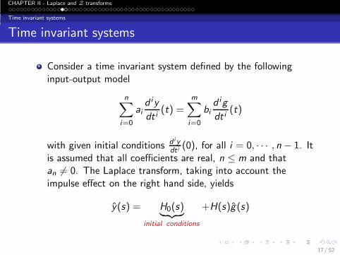
Consider a time invariant system defined by the followinginput-output model

n∑

i=0

aid iy

dt i(t) =

m∑

i=0

bid ig

dt i(t)

with given initial conditions d iy

dt i(0), for all i = 0, · · · , n − 1. It

is assumed that all coefficients are real, n ≤ m and thatan 6= 0. The Laplace transform, taking into account theimpulse effect on the right hand side, yields

y(s) = H0(s)︸︷︷︸

initial conditions

+H(s)g(s)

17 / 52




The main facts are as follows :

h0(t) := L−1(H0(s)) is the part of the solution dependingexclusively on the initial conditions.h(t) := L−1(H(s)) is the impulse response (under zero initialconditions). The function h(t) ∗ g(t) is the part of the solutiondepending exclusively on the input.

⇓

y(t) = h0(t) +

∫ t

0

h(t − τ)g(τ)dτ , ∀ t ≥ 0

From the state space realization (A,B,C ,D) we get

H0(s) := C (sI − A)−1x0 , H(s) := C (sI − A)−1B + D

18 / 52


Time varying systems


We consider the class of time varying systems characterized by

n∑

i=0

ai (t)d iy

dt i(t) = 0 , ∀ t ≥ 0

where :

The time varying coefficients are such that ai(t) = αi t + βi

with αi , βi ∈ R for all i = 1, · · · , n and αn 6= 0.

The initial conditions d iy

dt i(0), i = 0, · · · , n− 1 are not all zero.

The Laplace transform reveals that whenever s ∈ D(f ) it istrue that

L(tf (t)) = − d

dsf (s)

19 / 52




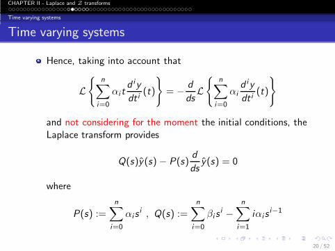
Hence, taking into account that

L{

n∑

i=0

αi td iy

dt i(t)

}

= − d

dsL{

n∑

i=0

αid iy

dt i(t)

}

and not considering for the moment the initial conditions, theLaplace transform provides

Q(s)y(s)− P(s)d

dsy(s) = 0

where

P(s) :=

n∑

i=0

αisi , Q(s) :=

n∑

i=0

βi si −

n∑

i=1

iαisi−1

20 / 52




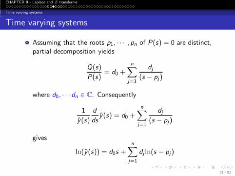
Assuming that the roots p1, · · · , pn of P(s) = 0 are distinct,partial decomposition yields

Q(s)

P(s)= d0 +

n∑

j=1

dj

(s − pj)

where d0, · · · dn ∈ C. Consequently

1

y(s)

d

dsy(s) = d0 +

n∑

j=1

dj

(s − pj)

gives

ln(y(s)) = d0s +

n∑

j=1

dj ln(s − pj)

21 / 52




The Laplace transform of the solution is

y(s) = ed0sn∏

j=1

(s − pj)dj

Important facts :

If d1, · · · , dn ∈ Z with∑n

j=1 dj ≤ 0 and d0 ≤ 0, the aboveproduct denoted H(s) is a rational function which provides

y(t) =

{0 0 ≤ t ≤ −d0

h(t + d0) t > −d0

The above solution y (s) may hold even though the initialconditions are not null.

22 / 52




Consider the Bessel differential equation

ty(t) + y(t) + ty(t) = 0 , y(0) = 1, y(0) = 0

From the same algebraic manipulations we get

1

y(s)

d

dsy(s) =

−1/2

(s + j)+

−1/2

(s − j)

⇓

y(s) =1√

s2 + 1, D(y) = {s ∈ C : Re(s) > 0}

and finally y(t) = J0(t) for all t ≥ 0 - the Bessel function.

23 / 52




Important facts :J0(t) is determined numerically by series expansion or bysolving the Bessel differential equation.The Bessel function has the following convolutional property

J0(t) ∗ J0(t) = sin(t) , ∀ t ≥ 0

0 2 4 6 8 10 12 14 16 18 20−0.5

0

0.5

1

J0

t

24 / 52


Nonrational transforms


An important function on this matter is the Γ-function,defined for all r > 0 by

Γ(r) :=

∫ ∞

0ξr−1e−ξdξ

Hence Γ(1) = 1 and

Γ(r + 1) = ξre−ξ∣∣0∞ + r

∫ ∞

0ξr−1e−ξdξ

= rΓ(r)

shows that for r ∈ N, Γ(r +1) = r !. It generalizes the factorialto positive real numbers. A particularly important value is

Γ(1/2) =√π

25 / 52




Considering the function g(t) := tr defined for all t > 0, andξ := st we have

g(s) =

∫ ∞

0tre−stdt

=Γ(r + 1)

sr+1

For all r > −1 ∈ R the Laplace transform of g(t) is given by

g(s) =Γ(r + 1)

sr+1, D(g) = {s ∈ C : Re(s) > 0}

This property holds even though r + 1 is not an integernumber. In this case g(s) is not rational.

26 / 52




Particular cases :

For r = 0, g(t) = υ(t) is the unit step function and theformula provides

g(s) =1

s

For r = −1/2, g(t) = 1/√t and the formula provides

g(s) =

√π√s

It can also be concluded that g(t) = 1/√πt exhibits the

following convolutional property

g(t) ∗ g(t) = υ(t) , ∀ t > 0

27 / 52


Z transform

Z transform

The Z transform of the function f (k) : Z → C denoted asf (z) or Z(f ) is a function of complex variable

f (z) : D(f ) → C

where D(f ) is its domain and

f (z) =

∞∑

k=−∞

f (k)z−k (3)

D(f ) := {z ∈ C : f (z) exists } (4)

It is important to keep in mind that f (z) exists means that thesum in (3) converges and is finite.

28 / 52


Z transform

Z transform

Generally D(f ) is a strict subset of C. In this case, there

exists z ∈ C such that z /∈ D(f ) and hence, the determination

of the domain D(f ) is an essential issue when dealing with Ztransform.

Important : The domain of the Z transform D(f ) stronglydepends on the domain of the function f (k). As it will be clearin the sequel :

k ∈ [0,+∞) =⇒ |z | ∈ (β,∞)

k ∈ (−∞, 0] =⇒ |z | ∈ (0, α)

k ∈ (−∞,∞) =⇒ |z | ∈ (β, α)

for some positive α, β ∈ R.

29 / 52


Z transform

Z transform

Define the complex sequence {z0, z1, z2, · · · } where z ∈ C

and notice thati−1∑

k=0

zk =1− z i

1− z, ∀ i ≥ 1

Using this we get the following result which is of particularimportance on Z transform calculations :

Lemma (Fundamental lemma)

Consider z ∈ C. The equality

∞∑

k=0

zk =1

1− z

holds and is finite if and only if |z | < 1.

30 / 52


Z transform

Z transform

For each function the Z transform (if any) is given :

f (k) = ak : Z → C and D(f ) = ∅.f (k) = ak : [0,+∞) → C and

f (z) =z

z − a, D(f ) = {z ∈ C : |z | > |a|}

f (k) = ak : (−∞, 0] → C and

f (z) = − a

z − a, D(f ) = {z ∈ C : |z | < |a|}

f (k) = a|k| : (−∞,+∞) → C and

f (z) =(a− 1/a)z

(z − a)(z − 1/a), D(f ) = {z ∈ C : |a| < |z | < 1/|a|}

31 / 52




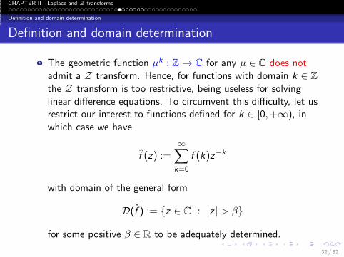
The geometric function µk : Z → C for any µ ∈ C does notadmit a Z transform. Hence, for functions with domain k ∈ Z

the Z transform is too restrictive, being useless for solvinglinear difference equations. To circumvent this difficulty, let usrestrict our interest to functions defined for k ∈ [0,+∞), inwhich case we have

f (z) :=∞∑

k=0

f (k)z−k

with domain of the general form

D(f ) := {z ∈ C : |z | > β}

for some positive β ∈ R to be adequately determined.

32 / 52




Important class : There exists zf ∈ C such that the limit

limℓ→∞

ℓ∑

k=0

|f (k)z−kf |

exists and is finite.

Lemma (Domain characterization)

For the functions of this class the following hold :

Any z ∈ C satisfying |z | ≥ |zf | belongs to D(f ).

There exists M finite such that |f (z)| ≤ M for all z ∈ D(f ).

33 / 52




General form : Functions defined for all k ≥ 0 ∈ Z :

D(f ) := {z ∈ C : |z | > β}

Domain determination : Given a function f (k), determine theminimum value of β ∈ R such that

limℓ→∞

ℓ∑

k=0

|f (k)z−kf | < ∞

Domain determination : Given a function f (z), determine theminimum value of β ∈ R such that f (z) remains analytic in allpoints of the complex plane belonging to D(f ).

34 / 52




Rational function :

f (z) :=N(z)

D(z)=

∑mi=0 biz

i

∑ni=0 aiz

i

where m ≤ n, bi ∈ R for all i = 1, · · · ,m and ai ∈ R for alli = 1, · · · , n. If m = n it is called proper otherwise strictlyproper. It is not analytic at the poles pi , i = 1, · · · , n roots ofD(z) = 0. Hence

β = maxi=1,··· ,n

|pi |

Unitary (Schur) impulse : δ(k) := 0k , k ∈ Z

δ(z) = 1 , D(δ) = C

35 / 52




Several calculations involving Z transform depend on theprecise determination of its domain :

Sum : The sum of a function f (k) defined for all k ≥ 0 can bedetermined from

∞∑

k=0

f (k) = f (1)

whenever 1 ∈ D(f ).Limit : The limit of a function f (k) defined for all k ≥ 0 canbe determined from

limk→∞

f (k) = limz→1

(z − 1)f (z)

whenever 1 ∈ D((z − 1)f ).

36 / 52



Properties

Basic properties for dynamic systems analysis, valid forfunctions defined in the time domain k ≥ 0 and scalarsθ1, θ2, · · · .

Linearity :

Z(∑

i

θi fi (k)

)

=∑

i

θi fi (z)

Discrete time convolution :

Z(f (k) • g(k)) = f (z)g (z)

Step ahead :

Z(f (k + 1)) = zf (z)− zf (0)

37 / 52



Properties

Discrete time convolution is essential for dynamic systemsanalysis, For functions f (k) and g(k) defined for allk ∈ [0,+∞) we have

f (k) • g(k) =k∑

i=0

f (k − i)g(i)

=

k∑

i=0

f (i)g(k − i) , ∀ k ≥ 0

applying to the discrete impulse function δ(k) we obtain :

f (k) • δ(k) = f (k) for all k ≥ 0.

Step function : υ(k) =∑k

i=0 δ(i) for all k ≥ 0.

38 / 52




Consider a time invariant system defined by the followinginput-output model

n∑

i=0

aiy(k + i) =

m∑

i=0

big(k + i)

with given initial conditions y(i), for all i = 0, · · · , n − 1. It isassumed that all coefficients are real, n ≤ m and that an 6= 0.The Z transform yields

y(z) = H0(z)︸︷︷︸

initial conditions

+H(z)g(z)

39 / 52




The main facts are as follows :

h0(k) := Z−1(H0(z)) is the part of the solution dependingexclusively on the initial conditions.h(k) := L−1(H(z)) is the impulse response (under zero initialconditions). The function h(k) • g(k) is the part of thesolution depending exclusively on the input.

⇓

y(k) = h0(k) +

k∑

i=0

h(k − i)g(i) , ∀ k ≥ 0

From the state space realization (A,B,C ,D) we get

H0(z) := zC (zI − A)−1x0 , H(z) := C (zI − A)−1B + D

40 / 52




We consider the class of time varying systems characterized by

n∑

i=0

ai(k)y(k + i) = 0 , ∀ k ≥ 0

where :

The time varying coefficients are such that ai(k) = αik + βi

with αi , βi ∈ R for all i = 1, · · · , n and αn 6= 0.The initial conditions y(i), i = 0, · · · , n − 1 are not all zero.

The Z transform reveals that whenever z ∈ D(f ) it is truethat

Z(kf (k)) = −zd

dzf (z)

41 / 52




Hence, taking into account that

Z{

n∑

i=0

αiky(k + i)

}

= −zd

dzZ{

n∑

i=0

αiy(k + i)

}

and not considering for the moment the initial conditions, theZ transform provides

Q(z)y(z)− P(z)d

dzy(z) = 0

where

P(z) :=

n∑

i=0

αizi+1 , Q(z) :=

n∑

i=0

βizi −

n∑

i=1

iαizi

42 / 52




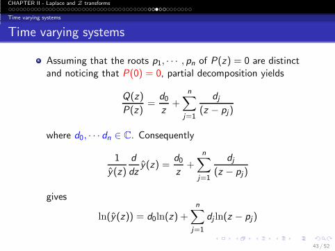
Assuming that the roots p1, · · · , pn of P(z) = 0 are distinctand noticing that P(0) = 0, partial decomposition yields

Q(z)

P(z)=

d0

z+

n∑

j=1

dj

(z − pj)

where d0, · · · dn ∈ C. Consequently

1

y(z)

d

dzy(z) =

d0

z+

n∑

j=1

dj

(z − pj)

gives

ln(y(z)) = d0ln(z) +n∑

j=1

dj ln(z − pj)

43 / 52




The Z transform of the solution is

y(z) = zd0n∏

j=1

(z − pj)dj

Important facts :

If d0, d1, · · · , dn ∈ Z with∑n

j=1 dj ≤ 0 and d0 ≤ 0, the aboveproduct denoted H(z) is a rational function which provides

y(k) =

{0 0 ≤ k < −d0

h(k + d0) k ≥ −d0

The above solution y (z) may hold even though the initialconditions are not null.

44 / 52




Consider the time varying difference equation

(k + 1)y(k + 1)− (k + 1/2)y(k) = 0 , y(0) = 1

From the same algebraic manipulations we get

1

y(z)

d

dzy(z) =

1/2

z+

−1/2

(z − 1)

⇓

y(z) =

√z

z − 1, D(y) = {z ∈ C : |z | > 1}

and finally y(k) • y(k) = υ(k) , ∀k ≥ 0. The function y(k)for all k ≥ 0, can be numerically calculated from the abovedifference equation.

45 / 52


Problems

Problems

1. Consider the Fibonacci difference equation

θ(k + 2)− θ(k + 1)− θ(k) = 0 , θ(0) = 0 , θ(1) = 1

Determine its solution θ(k) and the output θ(k + 1) + θ(k).Determine its state space representation.Determine the state space matrices such that the samesolution, delayed by one step, is obtained from zero initialcondition.

2. For a discrete time linear system with transfer function

G (z) =(z + 1)

(z + 1/2)(z − 1/2)

Determine its impulse response.

46 / 52


Problems

Problems

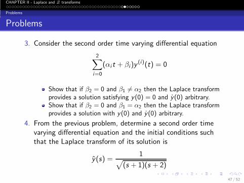
3. Consider the second order time varying differential equation

2∑

i=0

(αi t + βi)y(i)(t) = 0

Show that if β2 = 0 and β1 6= α2 then the Laplace transformprovides a solution satisfying y(0) = 0 and y(0) arbitrary.Show that if β2 = 0 and β1 = α2 then the Laplace transformprovides a solution with y(0) and y(0) arbitrary.

4. From the previous problem, determine a second order timevarying differential equation and the initial conditions suchthat the Laplace transform of its solution is

y(s) =1

√

(s + 1)(s + 2)

47 / 52


Problems

Problems

5. Consider z ∈ C. Prove that the equality

1

1− z=

∞∑

i=0

z i

holds if and only if |z | < 1. Using this result determine thefunction f (t) defined for all t ≥ 0 with Laplace transformgiven by:

f (s) = 1s(1−e−s) .

f (s) = 1(es−e−s) .

f (s) = e−s

(s+1)(1−e−s) .

48 / 52


Problems

Problems

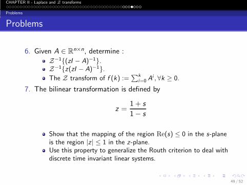
6. Given A ∈ Rn×n, determine :

Z−1{(zI − A)−1}.Z−1{z(zI − A)−1}.The Z transform of f (k) :=

∑k

i=0 Ai , ∀k ≥ 0.

7. The bilinear transformation is defined by

z =1 + s

1− s

Show that the mapping of the region Re(s) ≤ 0 in the s-planeis the region |z | ≤ 1 in the z-plane.Use this property to generalize the Routh criterion to deal withdiscrete time invariant linear systems.

49 / 52


Problems

Problems

8. Consider the matrices A ∈ Rn×n and B ∈ R

n×m. Using theLaplace transform, show that the square matrix

Γ :=

[A B

0 0

]

is such that

eΓt =

[eAt

∫ t

0 eAtBdt

0 I

]

9. Define the contour C to be used with the Nyquist criterion fordiscrete time systems stability analysis.

50 / 52


Problems

Problems

10. Consider the time delay system

y(t) + 3y(t) + 2y(t) + κy(t − T ) = u(t)

where κ ≥ 0 and T = 0, 1, 2. Using the Nyquist criterion,determine for each T the values of κ preserving asymptoticstability.

11. Consider a time delay system with transfer function

H(s) =1

s3 + 4s2 + 4s + κe−Ts

where κ,T ≥ 0. Determine the stability region (κ,T ) using:The Nyquist criterion.The Routh criterion adopting first and second orderapproximations to e−Ts .

51 / 52


Problems

Problems

12. Consider a time delay system with characteristic equation

P(s) + κe−Ts = 0

where κ,T ≥ 0. Assuming the roots of P(s) = 0 are in theregion Re(s) < 0, using the Nyquist criterion show thatasymptotic stability is preserved for all T ≥ 0, whenever

maxω≥0

κ

|P(jω)| < 1

Compare to the Nyquist criterion applied with the zero orderapproximation e−Ts = 1.

52 / 52

frequency domain analysis of dynamic systemsgeromel/rob_transf.pdf · chapter ii - laplace and z...

Documents