fractured gas well cases (lee and holditch, jpt · fractured gas well cases (lee and holditch, jpt...
TRANSCRIPT

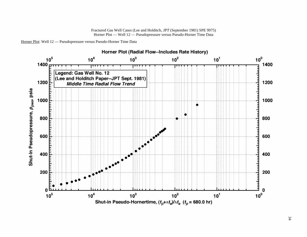
Fractured Gas Well Cases (Lee and Holditch, JPT (September 1981) SPE 9975)
Orientation:
This examination problem set concerns the analysis of pressure buildup tests in gas wells that have been hydraulically fractured. Note that the pseudopressure and pseudotime transformations are applied — you can simply analyze these well test data in the same manner as you would for data from an oil well test.
These tests are analyzed in some detail in the attached article by Lee and Holditch, but their analysis is by no means the "best" answer. Lee and Holditch did not have the benefit of the pressure derivative function — and their efforts were not uniquely focused on the use of the model for a vertical well with a finite conductivity vertical fracture. In short, use the analyses given by Lee and Holditch as a guide, but not as an answer that must be reproduced.
Required:
1. For this problem, you are to perform the following analyses:
"Preliminary" log-log analysis. Cartesian analysis of "early" time (wellbore storage distorted) data. Semilog analysis of "middle" time (radial flow) data. Log-log type curve analysis.
You are to complete the tables on the attached pages which are provided for you to tabulate your results. You should include any and all analyses and results you deem relevant — including, for example: extrapolated pressure from pressure buildup tests (pp*) and analyses using the Muskat plot (if applicable). Other analyses may also be relevant/appropriate — be sure to consider all the possibilities (this is an examination).
Notes:
a. Various type curves are provided in a 1 inch-by-1 inch format in this handout — these type curves should be sufficient for your analysis.
b. You are to provide a comprehensive HAND ANALYSIS of these test data — type curves are provided for hand analysis.

2
Fractured Gas Well Cases (Lee and Holditch, JPT (September 1981) SPE 9975) Governing Equations
Pseudopressure-Pseudotime Relations:
Pseudopressure: Pseudotime:
⎮⌡
⌠=
p
pdp
zp
pz
pbase gi
igip
μ
μ
⎮⌡
⌠ΔΔ=Δ
ttd
ticgit ticgia
0 1
μμ
Early-Time Cartesian Analysis: (pseudopressure-pseudotime form)
.24
yields which ,24
where,)(or 0)( wbs
gigs
s
gigwbsaeawbspwfpws m
BqC
CBq
mttmtpp ==ΔΔ+=Δ=
Semilog Analysis: (pseudopressure-pseudotime form)
Horner:
.6.162 gives which ,6.162 where, ln hm
Bqk
khBq
mt
ttmpp
sl
gigiggigigsl
a
apslpipws
μμ==
⎥⎥⎦
⎤
⎢⎢⎣
⎡
Δ
Δ+−=
and the skin factor, s, is given by:
⎥⎥⎥
⎦
⎤
⎢⎢⎢
⎣
⎡+
⎥⎥⎥
⎦
⎤
⎢⎢⎢
⎣
⎡−
⎥⎥⎦
⎤
⎢⎢⎣
⎡
+−
=Δ−=Δ= 2275.3
2log
1log
0))(hr) 1((1513.1
wrticgi
kt
t
slmatpwfpatpwsp
sp
p
φμ
MDH:
.6.162 where,8686.02275.32
log )ln( 0)(kh
Bqms
wrticgi
kmtmtpp gigigslslaslapwfpws
μ
φμ=
⎥⎥⎥
⎦
⎤
⎢⎢⎢
⎣
⎡+−
⎥⎥⎥
⎦
⎤
⎢⎢⎢
⎣
⎡+Δ+=Δ=
where the formation permeability, k, and the skin factor, s, are given by:
hmBq
ksl
gigig μ6.162= and
⎥⎥⎥
⎦
⎤
⎢⎢⎢
⎣
⎡+
⎥⎥⎥
⎦
⎤
⎢⎢⎢
⎣
⎡−
=Δ−=Δ= 2275.3
2log
0))(hr) 1((1513.1
wrticgi
k
slmatpwfpatpwsp
sφμ
Type Curve Analysis Relations: (pseudopressure-pseudotime form)
"Bourdet -Gringarten" Type Curves: "Economides" Type Curves: (Unfractured Vertical Well with (Fractured Vertical Well with Wellbore Storage and Skin Effects) Wellbore Storage Effects)
Family Parameter: CDe2s Family Parameter: CDf
Formation Permeability: Formation Permeability:
]or [
]or [ 2.141MP
'pp
MP'wDwDgigig
pp
pph
Bqk
ΔΔ=
μ ]or [
]or [ 2.141MP
'pp
MP'wDwDgigig
pp
pph
Bqk
ΔΔ=
μ
Dimensionless Wellbore Storage Coefficient: Fracture Half-Length:
]/[
]or [ 0002637.0 2 MPDDMPaea
wtigiD Ct
tt
rc
kC ΔΔ=
φμ
]/[]or [1 0002637.02
MPDfDxfMPaea
Dftigif Ct
ttCc
kx ΔΔ=
φμ
Skin Factor:
][ln21
2
⎥⎥⎦
⎤
⎢⎢⎣
⎡=
DMP
sD
CeCs

3
Fractured Gas Well Cases (Lee and Holditch, JPT (September 1981) SPE 9975) Required Results — Lee and Holditch Well 5 (SPE 9975)
Required: Lee and Holditch Well 5 (SPE 9975)
You are to estimate the following:
"Preliminary" log-log analysis: a. The wellbore storage coefficient, Cs. b. The dimensionless wellbore storage coefficient, CDf (based on xf).* c. The formation permeability, k.
Cartesian analysis of "early" time (wellbore storage distorted) data: a. The pseudopressure at the start of the test, ppws(Δt=0). b. The wellbore storage coefficient, Cs. c. The dimensionless wellbore storage coefficient, CDf (based on xf).*
Semilog analysis of "middle" time (radial flow) data: (use both Horner and MDH methods) a. The formation permeability, k. b. The near well skin factor, s. c. The radius of investigation, rinv, at the end of radial flow or the end of the test data.
Log-log type curve analysis: (use Δtae methods) a. The dimensionless fracture conductivity, CfD. b. The formation permeability, k. c. The fracture half-length, xf. d. The wellbore storage coefficient, Cs. e. The dimensionless wellbore storage coefficient, CD.* f. The pseudoradial flow skin factor, spr.
* If the fractured well model is applicable — if not, document the well model and provide analysis based on that presumed model. In general, all plausible results should be provided, with an appropriate level of supporting documentation.
Results: Lee and Holditch Well 5 (SPE 9975)
Log-log Analysis:
Wellbore storage coefficient, Cs = RB/psi
Dimensionless wellbore storage coefficient, CDf (based on xf) =
Formation permeability, k = md
Cartesian Analysis: Early Time Data
Pressure drop at the start of the test, ppws(Δt=0) = psi
Wellbore storage coefficient, Cs = RB/psi
Dimensionless wellbore storage coefficient, CDf (based on xf) =
Semilog Analysis: Horner Δta (MDH)
Formation permeability, k = md = md
Near well skin factor, s = =
Radius of investigation, rinv (end of radial flow or end of test) = ft = ft
Log-Log Type Curve Analysis: Δtae Δta
Dimensionless fracture conductivity, CfD = =
Formation permeability, k = md = md
Fracture half-length, xf = ft = ft
Wellbore storage coefficient, Cs = RB/psi = RB/psi
Dimensionless wellbore storage coefficient, CDf (based on xf) = =
Pseudoradial flow skin factor, spr = =

4
Fractured Gas Well Cases (Lee and Holditch, JPT (September 1981) SPE 9975) Required Results — Lee and Holditch Well 10 (SPE 9975)
Required: Lee and Holditch Well 10 (SPE 9975)
You are to estimate the following:
"Preliminary" log-log analysis: a. The wellbore storage coefficient, Cs. b. The dimensionless wellbore storage coefficient, CDf (based on xf).* c. The formation permeability, k.
Cartesian analysis of "early" time (wellbore storage distorted) data: a. The pseudopressure at the start of the test, ppws(Δt=0). b. The wellbore storage coefficient, Cs. c. The dimensionless wellbore storage coefficient, CDf (based on xf).*
Semilog analysis of "middle" time (radial flow) data: (use both Horner and MDH methods) a. The formation permeability, k. b. The near well skin factor, s. c. The radius of investigation, rinv, at the end of radial flow or the end of the test data.
Log-log type curve analysis: (use Δtae methods) a. The dimensionless fracture conductivity, CfD. b. The formation permeability, k. c. The fracture half-length, xf. d. The wellbore storage coefficient, Cs. e. The dimensionless wellbore storage coefficient, CD.* f. The pseudoradial flow skin factor, spr.
* If the fractured well model is applicable — if not, document the well model and provide analysis based on that presumed model. In general, all plausible results should be provided, with an appropriate level of supporting documentation.
Results: Lee and Holditch Well 10 (SPE 9975)
Log-log Analysis:
Wellbore storage coefficient, Cs = RB/psi
Dimensionless wellbore storage coefficient, CDf (based on xf) =
Formation permeability, k = md
Cartesian Analysis: Early Time Data
Pressure drop at the start of the test, ppws(Δt=0) = psi
Wellbore storage coefficient, Cs = RB/psi
Dimensionless wellbore storage coefficient, CDf (based on xf) =
Semilog Analysis: Horner Δta (MDH)
Formation permeability, k = md = md
Near well skin factor, s = =
Radius of investigation, rinv (end of radial flow or end of test) = ft = ft
Log-Log Type Curve Analysis: Δtae Δta
Dimensionless fracture conductivity, CfD = =
Formation permeability, k = md = md
Fracture half-length, xf = ft = ft
Wellbore storage coefficient, Cs = RB/psi = RB/psi
Dimensionless wellbore storage coefficient, CDf (based on xf) = =
Pseudoradial flow skin factor, spr = =

5
Fractured Gas Well Cases (Lee and Holditch, JPT (September 1981) SPE 9975) Required Results — Lee and Holditch Well 12 (SPE 9975)
Required: Lee and Holditch Well 12 (SPE 9975)
You are to estimate the following:
"Preliminary" log-log analysis: a. The wellbore storage coefficient, Cs. b. The dimensionless wellbore storage coefficient, CDf (based on xf).* c. The formation permeability, k.
Cartesian analysis of "early" time (wellbore storage distorted) data: a. The pseudopressure at the start of the test, ppws(Δt=0). b. The wellbore storage coefficient, Cs. c. The dimensionless wellbore storage coefficient, CDf (based on xf).*
Semilog analysis of "middle" time (radial flow) data: (use both Horner and MDH methods) a. The formation permeability, k. b. The near well skin factor, s. c. The radius of investigation, rinv, at the end of radial flow or the end of the test data.
Log-log type curve analysis: (use Δtae methods) a. The dimensionless fracture conductivity, CfD. b. The formation permeability, k. c. The fracture half-length, xf. d. The wellbore storage coefficient, Cs. e. The dimensionless wellbore storage coefficient, CD.* f. The pseudoradial flow skin factor, spr.
* If the fractured well model is applicable — if not, document the well model and provide analysis based on that presumed model. In general, all plausible results should be provided, with an appropriate level of supporting documentation.
Results: Lee and Holditch Well 12 (SPE 9975)
Log-log Analysis:
Wellbore storage coefficient, Cs = RB/psi
Dimensionless wellbore storage coefficient, CDf (based on xf) =
Formation permeability, k = md
Cartesian Analysis: Early Time Data
Pressure drop at the start of the test, ppws(Δt=0) = psi
Wellbore storage coefficient, Cs = RB/psi
Dimensionless wellbore storage coefficient, CDf (based on xf) =
Semilog Analysis: Horner Δta (MDH)
Formation permeability, k = md = md
Near well skin factor, s = =
Radius of investigation, rinv (end of radial flow or end of test) = ft = ft
Log-Log Type Curve Analysis: Δtae Δta
Dimensionless fracture conductivity, CfD = =
Formation permeability, k = md = md
Fracture half-length, xf = ft = ft
Wellbore storage coefficient, Cs = RB/psi = RB/psi
Dimensionless wellbore storage coefficient, CDf (based on xf) = =
Pseudoradial flow skin factor, spr = =

6
Fractured Gas Well Cases (Lee and Holditch, JPT (September 1981) SPE 9975) "Cinco-Samaniego" Type Curve
"Cinco-Samaniego" Type Curve: pwD and pwD' vs. tDxf — Various CfD Values (NO WELLBORE STORAGE EFFECTS) (1"x1" format)
7
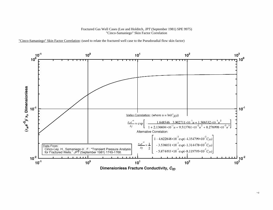
Fractured Gas Well Cases (Lee and Holditch, JPT (September 1981) SPE 9975) "Cinco-Samaniego" Skin Factor Correlation
"Cinco-Samaniego" Skin Factor Correlation: (used to relate the fractured well case to the Pseudoradial flow skin factor)

8
Fractured Gas Well Cases (Lee and Holditch, JPT (September 1981) SPE 9975) Bourdet-Gringarten Type Curve (Unfractured Well)
Bourdet-Gringarten Type Curve: pwD and pwD' vs. tD/CD — Various CD Values (Radial Flow Case — Includes Wellbore Storage and Skin Effects) (1"x1" format)

9
Fractured Gas Well Cases (Lee and Holditch, JPT (September 1981) SPE 9975) "Economides" Type Curve (CfD =1, CDf =various)
"Economides" Type Curve: pwD and pwD' vs. tDxf/CDf — CfD =1 (Fractured Well Case — Includes Wellbore Storage Effects) (1"x1" format)

10
Fractured Gas Well Cases (Lee and Holditch, JPT (September 1981) SPE 9975) "Economides" Type Curve (CfD =2, CDf =various)
"Economides" Type Curve: pwD and pwD' vs. tDxf/CDf — CfD =2 (Fractured Well Case — Includes Wellbore Storage Effects) (1"x1" format)

11
Fractured Gas Well Cases (Lee and Holditch, JPT (September 1981) SPE 9975) "Economides" Type Curve (CfD =2, CDf =various)
"Economides" Type Curve: pwD and pwD' vs. tDxf/CDf — CfD =5 (Fractured Well Case — Includes Wellbore Storage Effects) (1"x1" format)

12
Fractured Gas Well Cases (Lee and Holditch, JPT (September 1981) SPE 9975) "Economides" Type Curve (CfD =10, CDf =various)
"Economides" Type Curve: pwD and pwD' vs. tDxf/CDf — CfD =10 (Fractured Well Case — Includes Wellbore Storage Effects) (1"x1" format)

13
Fractured Gas Well Cases (Lee and Holditch, JPT (September 1981) SPE 9975) "Economides" Type Curve (CfD =1x10⁻³, CDf =various)
"Economides" Type Curve: pwD and pwD' vs. tDxf/CDf — CfD =1x10⁻³ (Fractured Well Case — Includes Wellbore Storage Effects) (1"x1" format)

14
Fractured Gas Well Cases (Lee and Holditch, JPT (September 1981) SPE 9975) Ansah Type Curve — Pressure Buildup in a Bounded (Closed) Reservoir System
Ansah Type Curve: Pressure Buildup in a Bounded (Closed) Reservoir System (1"x1" format)

15
Fractured Gas Well Cases (Lee and Holditch, JPT (September 1981) SPE 9975) Stewart Type Curve — Well in an Infinite-Acting Reservoir System with a Single or Multiple Sealing Faults
Stewart Type Curve: Well in an Infinite-Acting Reservoir System with a Single or Multiple Sealing Faults. (1"x1" format)

16
Fractured Gas Well Cases (Lee and Holditch, JPT (September 1981) SPE 9975) Data Inventory — Wells 5, 10, and 12 (Lee and Holditch (SPE 9975))
Field Cases:
Case 1: Well 5 (Lee and Holditch, JPT (September 1981))
Reservoir properties: φ = 0.03 h = 30 ft rw = 0.33 ft (assumed)
Gas properties: (at the initial reservoir pressure (pi) of 8800 psia) γg = 0.6 (air=1) T= 325 deg F Bgi = 0.5755 RB/MSCF μgi = 0.0297 cp ct = cgi = 6.37x10⁻⁵ psia-1
Production parameters: ppwf(Δt=0) = 3456.8 psia qg = 1,500 MSCF/D (constant) tp = 180.8 hr
Case 2: Well 10 (Lee and Holditch, JPT (September 1981))
Reservoir properties: φ = 0.057 h = 27 ft rw = 0.33 ft (assumed)
Gas properties: (at the initial reservoir pressure (pi) of 9,950 psia) γg = 0.6 (air=1) T= 308 deg F Bgi = 0.5282 RB/MSCF μgi = 0.0317 cp ct = cgi = 5.10x10⁻⁵ psia-1
Production parameters: ppwf(Δt=0) = 1518.2 psia qg = 1,300 MSCF/D (constant) tp = 144 hr
Case 3: Well 12 (Lee and Holditch, JPT (September 1981))
Reservoir properties: φ = 0.045 h = 45 ft rw = 0.33 ft (assumed)
Gas properties: (at the initial reservoir pressure(pi) of 2200 psia) γg = 0.7 (air=1) T= 180 deg F Bgi = 1.2601 RB/MSCF μgi = 0.0174 cp ct = cgi = 4.64x10⁻⁴ psia-1
Production parameters: ppwf(Δt=0) = 8.2597 psia qg = 325 MSCF/D (constant) tp = 680 hr
Reference(s):
1. Lee, W.J. and Holditch, S.A.: "Fracture Evaluation With Pressure Transient Testing in Low-Perme-ability Gas Reservoirs," JPT (September 1981), 1776-1792.

17
Fractured Gas Well Cases (Lee and Holditch, JPT (September 1981) SPE 9975) Well Test Data Functions — Well 5 — Lee and Holditch, JPT (September 1981)
Well Test Data Functions: Well 5 — Lee and Holditch, JPT (September 1981)
Point Δt, hr pws, psia Δta, hr Δtae, hr ppws, psia Δpp, psi Δpp'(Δta), psi Δpp'(Δtae), psi1 0.0333 5869 0.0209 0.0209 3470.57 13.77 8.02 8.032 0.0667 5875 0.0420 0.0420 3476.17 19.37 22.90 22.913 0.1000 5893 0.0631 0.0631 3492.96 36.16 36.16 36.184 0.1667 5917 0.1055 0.1054 3515.35 58.55 51.65 51.695 0.2667 5947 0.1694 0.1692 3543.34 86.54 63.37 63.436 0.3333 5959 0.2122 0.2120 3554.53 97.73 67.29 67.387 0.5000 5994 0.3196 0.3190 3587.19 130.39 77.71 77.868 0.6667 6018 0.4277 0.4267 3609.58 152.78 92.08 92.379 0.8333 6041 0.5362 0.5346 3631.04 174.24 97.11 97.46
10 1.0000 6059 0.6451 0.6428 3647.83 191.03 105.93 106.4011 2.0000 6154 1.3063 1.2969 3736.46 279.66 157.64 159.0512 3.0000 6231 1.9780 1.9566 3809.55 352.75 205.00 207.9713 4.0000 6296 2.6578 2.6193 3871.33 414.53 227.96 232.0314 6.0000 6414 4.0389 3.9506 3983.49 526.69 284.80 292.2315 8.0000 6497 5.4446 5.2854 4062.38 605.58 345.23 357.4216 9.0000 6544 6.1558 5.9531 4107.06 650.26 368.29 383.2517 11.0000 6627 7.5950 7.2888 4186.33 729.53 395.89 415.4118 13.0000 6710 9.0542 8.6224 4266.40 809.60 436.69 460.4819 15.0000 6781 10.5314 9.9517 4334.90 878.10 463.86 493.5720 17.0000 6846 12.0249 11.2750 4397.60 940.80 478.27 511.6821 19.0000 6905 13.5340 12.5915 4454.52 997.72 490.57 530.3122 21.0000 6959 15.0576 13.9000 4506.61 1049.81 502.99 548.2423 23.0000 7018 16.5962 15.2009 4563.53 1106.73 518.32 572.2724 25.0000 7065 18.1486 16.4930 4609.16 1152.36 530.99 594.9625 27.0000 7107 19.7117 17.7739 4650.16 1193.36 547.23 606.7326 29.0000 7148 21.2844 19.0426 4690.18 1233.38 551.78 625.5627 31.0000 7183 22.8661 20.2989 4724.34 1267.54 565.36 641.5628 34.0000 7243 25.2559 22.1603 4782.91 1326.11 579.00 663.7329 37.0000 7302 27.6679 23.9958 4840.50 1383.70 581.64 679.1830 39.0000 7337 29.2877 25.2048 4874.66 1417.86 581.84 676.2431 42.0000 7391 31.7349 26.9964 4927.37 1470.57 590.90 690.5632 45.0000 7432 34.2010 28.7605 4967.39 1510.59 588.91 696.7333 48.0000 7479 36.6851 30.4971 5013.27 1556.47 602.75 709.9334 51.0000 7521 39.1862 32.2060 5054.63 1597.83 603.12 724.7835 54.0000 7562 41.7019 33.8860 5095.03 1638.23 608.12 729.0736 57.0000 7598 44.2312 35.5373 5130.49 1673.69 606.37 735.2037 59.0000 7621 45.9244 36.6221 5153.15 1696.35 605.35 735.6938 61.0000 7639 47.6227 37.6941 5170.88 1714.08 601.67 732.4939 63.0000 7663 49.3261 38.7534 5194.53 1737.73 603.51 736.5040 65.0000 7681 51.0348 39.8003 5212.26 1755.46 596.76 734.5641 67.0000 7698 52.7478 40.8345 5229.01 1772.21 593.66 734.42

18
Fractured Gas Well Cases (Lee and Holditch, JPT (September 1981) SPE 9975) Cartesian Plot — Well 5 — Early-Time Pseudopressure versus Pseudotime Data
Cartesian Plot: Well 5 — Early-Time Pseudopressure versus Pseudotime Data

19
Fractured Gas Well Cases (Lee and Holditch, JPT (September 1981) SPE 9975) Semilog Plot — Well 5 — "MDH" Plot — Pseudopressure versus Pseudotime Data
Semilog Plot: Well 5 — "MDH" Plot — Pseudopressure versus Pseudotime Data

20
Fractured Gas Well Cases (Lee and Holditch, JPT (September 1981) SPE 9975) Horner Plot — Well 5 — Pseudopressure versus Pseudo-Horner Time Data
Horner Plot: Well 5 — Pseudopressure versus Pseudo-Horner Time Data

21
Fractured Gas Well Cases (Lee and Holditch, JPT (September 1981) SPE 9975) Muskat Plot — Well 5 — Pseudopressure versus Pseudopressure Derivative Data
Muskat Plot: Well 5 — Pseudopressure versus Pseudopressure Derivative Data

22
Fractured Gas Well Cases (Lee and Holditch, JPT (September 1981) SPE 9975) Log-log Plot — Well 5 — Pseudopressure Drop and Pseudopressure Drop Derivative Data Versus Shut-In Pseudotime (1 inch x 1 inch)
Log-log Plot: Well 5 — Pseudopressure Drop and Pseudopressure Drop Derivative Data Versus Shut-In Pseudotime (1 inch x 1 inch)

23
Fractured Gas Well Cases (Lee and Holditch, JPT (September 1981) SPE 9975) Log-log Plot — Well 5 — Pseudopressure Drop and Pseudopressure Drop Derivative Data Versus Shut-In Effective Pseudotime (1 inch x 1 inch)
Log-log Plot: Well 5 — Pseudopressure Drop and Pseudopressure Drop Derivative Data Versus Shut-In Effective Pseudotime (1 inch x 1 inch)

24
Fractured Gas Well Cases (Lee and Holditch, JPT (September 1981) SPE 9975) Well Test Data Functions — Well 10 — Lee and Holditch, JPT (September 1981)
Well Test Data Functions: Well 10 — Lee and Holditch, JPT (September 1981)
Point Δt, hr pws, psia Δta, hr Δtae, hr ppws, psia Δpp, psi Δpp'(Δta), psi Δpp'(Δtae), psi1 0.0167 3589 0.0052 0.0052 1553.49 35.29 77.58 77.592 0.0333 3643 0.0081 0.0081 1595.53 77.33 70.58 70.593 0.0500 3701 0.0160 0.0160 1640.69 122.49 133.66 133.684 0.0833 3829 0.0273 0.0273 1740.34 222.14 177.37 177.405 0.1333 3936 0.0447 0.0447 1823.64 305.44 197.99 198.076 0.2500 4130 0.0872 0.0871 1982.26 464.06 387.19 387.497 0.3333 4321 0.1189 0.1188 2140.63 622.43 538.73 539.378 0.4167 4474 0.1522 0.1520 2267.48 749.28 659.47 660.299 0.5000 4638 0.1867 0.1865 2409.98 891.78 876.50 877.96
10 0.6667 4967 0.2599 0.2594 2696.14 1177.94 1147.91 1150.3911 0.8333 5394 0.3393 0.3385 3081.09 1562.89 1279.20 1282.5512 1.0000 5761 0.4255 0.4242 3419.54 1901.34 1372.29 1376.3713 1.2500 6167 0.5646 0.5624 3800.12 2281.92 1587.93 1594.9414 1.5000 6459 0.7132 0.7097 4076.83 2558.63 1316.55 1323.8915 1.7500 6857 0.8711 0.8659 4460.03 2941.83 1348.38 1356.7916 2.0000 7309 1.0402 1.0327 4899.43 3381.23 1281.78 1289.5617 3.0000 7759 1.7663 1.7449 5340.78 3822.58 724.86 733.3818 4.0000 7923 2.5267 2.4831 5502.13 3983.93 743.47 757.9019 5.0000 8138 3.3083 3.2340 5714.81 4196.61 631.75 647.5820 6.0000 8306 4.1109 3.9968 5881.18 4362.98 677.28 695.7921 8.0000 8509 5.7585 5.5371 6082.44 4564.24 562.81 604.8522 10.0000 8637 7.4434 7.0776 6209.78 4691.58 513.46 540.3623 12.0000 8732 9.1524 8.6055 6304.29 4786.09 484.42 542.2924 14.0000 8822 10.8826 10.1180 6393.82 4875.62 457.60 493.1725 16.0000 8891 12.6315 11.6128 6462.47 4944.27 445.37 478.3926 18.0000 8958 14.3969 13.0884 6529.13 5010.93 415.09 459.1627 21.0000 9040 17.0702 15.2611 6610.94 5092.74 397.40 450.1828 25.0000 9096 20.6638 18.0707 6666.82 5148.62 379.10 438.4429 28.0000 9135 23.3745 20.1102 6705.73 5187.53 358.03 419.5430 31.0000 9172 26.0977 22.0936 6742.65 5224.45 338.84 399.3131 34.0000 9207 28.8330 24.0229 6777.57 5259.37 311.99 382.3632 37.0000 9237 31.5794 25.8996 6807.51 5289.31 297.59 356.8233 40.0000 9270 34.3367 27.7256 6840.43 5322.23 296.14 363.1934 43.0000 9298 37.1046 29.5026 6868.37 5350.17 288.75 378.9035 46.0000 9323 39.8819 31.2320 6893.31 5375.11 288.26 378.4336 52.0000 9350 45.4550 34.5492 6920.25 5402.05 272.11 370.0437 55.0000 9365 48.2492 36.1400 6935.22 5417.02 266.89 368.6638 58.0000 9372 51.0473 37.6873 6942.20 5424.00 254.91 359.0239 61.0000 9384 53.8489 39.1927 6954.18 5435.98 250.74 353.0340 64.0000 9396 56.6549 40.6584 6966.15 5447.95 239.41 351.5441 67.0000 9404 59.4646 42.0855 6974.13 5455.93 225.72 343.9842 70.0000 9416 62.2780 43.4755 6986.11 5467.91 227.36 344.81

25
Fractured Gas Well Cases (Lee and Holditch, JPT (September 1981) SPE 9975) Cartesian Plot — Well 10 — Early-Time Pseudopressure versus Pseudotime Data
Cartesian Plot: Well 10 — Early-Time Pseudopressure versus Pseudotime Data

26
Fractured Gas Well Cases (Lee and Holditch, JPT (September 1981) SPE 9975) Semilog Plot — Well 10 — "MDH" Plot — Pseudopressure versus Pseudotime Data
Semilog Plot: Well 10 — "MDH" Plot — Pseudopressure versus Pseudotime Data

27
Fractured Gas Well Cases (Lee and Holditch, JPT (September 1981) SPE 9975) Horner Plot — Well 10 — Pseudopressure versus Pseudo-Horner Time Data
Horner Plot: Well 10 — Pseudopressure versus Pseudo-Horner Time Data

28
Fractured Gas Well Cases (Lee and Holditch, JPT (September 1981) SPE 9975) Muskat Plot — Well 10 — Pseudopressure versus Pseudopressure Derivative Data
Muskat Plot: Well 10 — Pseudopressure versus Pseudopressure Derivative Data
29
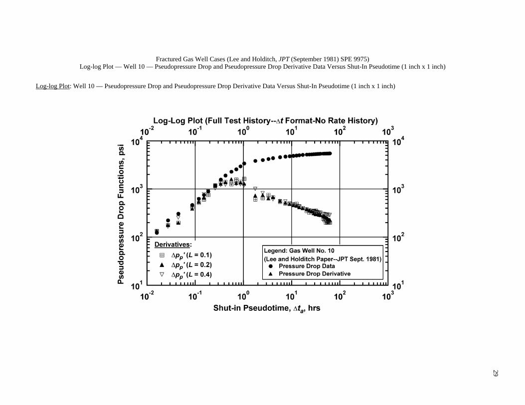
Fractured Gas Well Cases (Lee and Holditch, JPT (September 1981) SPE 9975) Log-log Plot — Well 10 — Pseudopressure Drop and Pseudopressure Drop Derivative Data Versus Shut-In Pseudotime (1 inch x 1 inch)
Log-log Plot: Well 10 — Pseudopressure Drop and Pseudopressure Drop Derivative Data Versus Shut-In Pseudotime (1 inch x 1 inch)

30
Fractured Gas Well Cases (Lee and Holditch, JPT (September 1981) SPE 9975) Log-log Plot: Well 10 — Pseudopressure Drop and Pseudopressure Drop Derivative Data Versus Shut-In Effective Pseudotime (1 inch x 1 inch)
Log-log Plot: Well 10 — Pseudopressure Drop and Pseudopressure Drop Derivative Data Versus Shut-In Effective Pseudotime (1 inch x 1 inch)

31
Fractured Gas Well Cases (Lee and Holditch, JPT (September 1981) SPE 9975)
Well Test Data Functions — Well 12 — Lee and Holditch, JPT (September 1981)
Well Test Data Functions: Well 12 — Lee and Holditch, JPT (September 1981)
Point Δt, hr pws, psia Δta, hr Δtae, hr ppws, psia Δpp, psi Δpp'(Δta), psi Δpp'(Δtae), psi1 0.0083 190 0.0004 0.0004 10.27 2.01 7.57 7.572 0.0167 270 0.0015 0.0015 20.27 12.01 9.44 9.443 0.0250 319 0.0030 0.0030 27.49 19.23 15.43 15.434 0.0333 365 0.0046 0.0046 36.33 28.07 20.93 20.935 0.0500 438 0.0085 0.0085 51.40 43.14 31.29 31.296 0.0667 500 0.0131 0.0131 67.73 59.47 42.03 42.037 0.0833 551 0.0181 0.0181 81.33 73.07 50.32 50.328 0.1000 597 0.0235 0.0235 96.22 87.96 55.18 55.189 0.1167 636 0.0293 0.0293 108.86 100.60 61.33 61.33
10 0.1333 670 0.0354 0.0354 120.45 112.19 65.24 65.2411 0.1667 726 0.0484 0.0484 141.83 133.57 71.91 71.9112 0.2000 774 0.0621 0.0621 160.38 152.12 78.22 78.2213 0.2333 815 0.0766 0.0766 178.37 170.11 82.49 82.4914 0.2667 848 0.0917 0.0917 192.85 184.59 88.60 88.6015 0.3000 880 0.1072 0.1072 206.89 198.63 90.63 90.6316 0.3333 906 0.1232 0.1232 219.75 211.49 93.59 93.5917 0.4000 955 0.1563 0.1563 243.99 235.73 100.19 100.1918 0.4667 992 0.1907 0.1907 262.40 254.14 104.84 104.8419 0.5333 1027 0.2261 0.2261 281.63 273.37 109.29 109.2920 0.6000 1057 0.2625 0.2625 298.10 289.84 110.89 110.8921 0.6667 1084 0.2997 0.2997 312.93 304.67 114.68 114.6822 0.8000 1131 0.3761 0.3761 340.39 332.13 121.44 121.4423 0.9333 1171 0.4608 0.4608 364.48 356.22 126.95 126.9524 1.0667 1206 0.5418 0.5418 385.56 377.30 131.39 131.3925 1.2000 1236 0.6244 0.6244 404.97 396.71 134.62 134.6226 1.4667 1287 0.7941 0.7941 438.30 430.04 140.65 140.6527 1.7333 1330 0.9688 0.9688 466.90 458.64 146.47 146.4728 2.0000 1366 1.1478 1.1478 492.21 483.95 148.73 148.7329 2.2667 1396 1.3301 1.3301 513.30 505.04 152.07 152.0730 2.6000 1433 1.5624 1.5624 539.46 531.20 150.92 150.9231 3.0000 1467 1.8468 1.8468 564.97 556.71 159.90 159.9032 3.4000 1498 2.1360 2.1360 588.23 579.97 157.23 157.2333 3.8000 1523 2.4296 2.4296 606.99 598.73 160.10 160.1034 4.2000 1544 2.7269 2.7269 622.93 614.67 157.65 157.6535 4.6000 1575 3.0281 3.0281 647.59 639.33 166.32 166.3236 5.0000 1590 3.3327 3.3327 659.52 651.26 164.06 164.0637 5.4000 1605 3.6396 3.6396 671.45 663.19 163.44 163.4438 5.8000 1624 3.9491 3.9491 686.56 678.30 167.34 167.3439 10.4000 1761 7.6467 7.6467 800.32 792.06 127.62 127.6240 16.0000 1813 12.3488 12.3488 846.00 837.74 124.26 124.2641 29.1667 1933 23.8318 23.8318 953.80 945.54 163.96 163.96
32
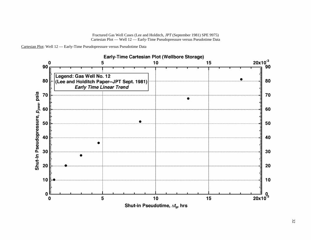
Fractured Gas Well Cases (Lee and Holditch, JPT (September 1981) SPE 9975) Cartesian Plot — Well 12 — Early-Time Pseudopressure versus Pseudotime Data
Cartesian Plot: Well 12 — Early-Time Pseudopressure versus Pseudotime Data
33
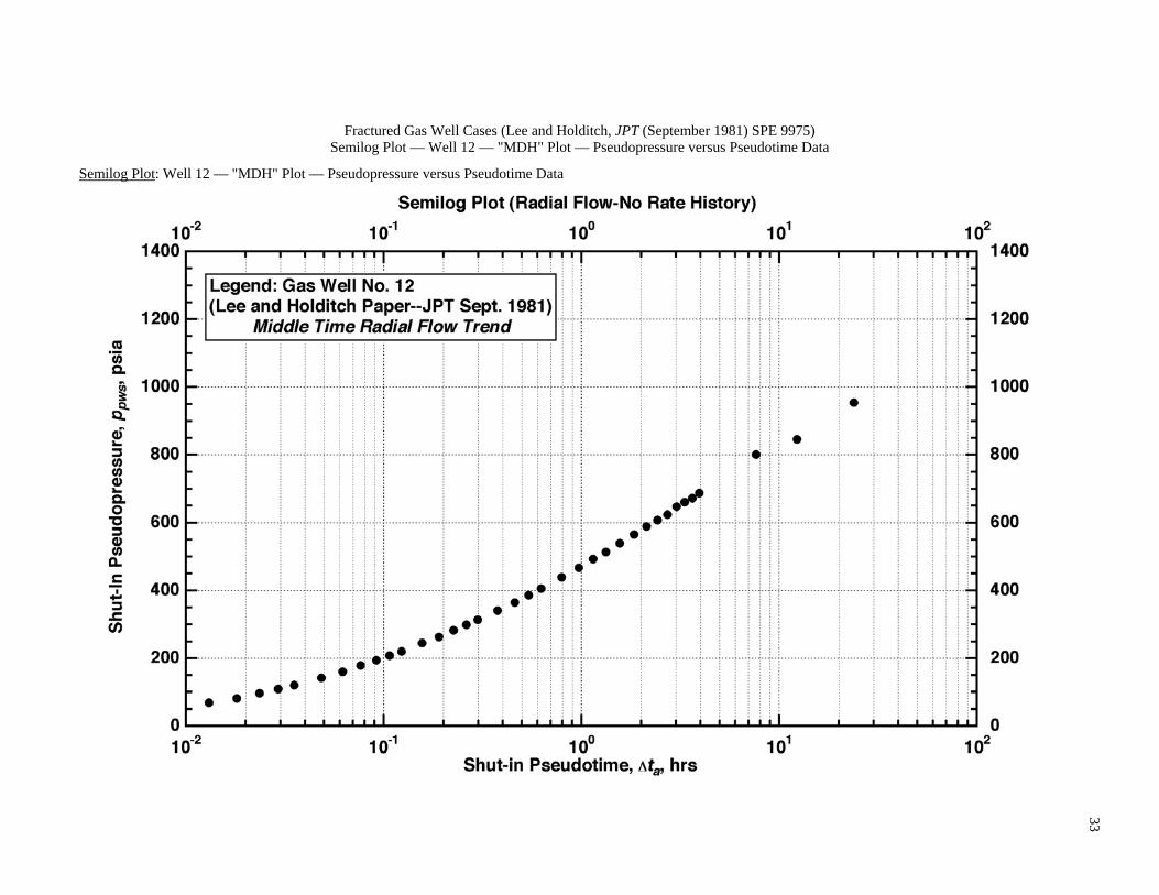
Fractured Gas Well Cases (Lee and Holditch, JPT (September 1981) SPE 9975) Semilog Plot — Well 12 — "MDH" Plot — Pseudopressure versus Pseudotime Data
Semilog Plot: Well 12 — "MDH" Plot — Pseudopressure versus Pseudotime Data
34
Fractured Gas Well Cases (Lee and Holditch, JPT (September 1981) SPE 9975)
Horner Plot — Well 12 — Pseudopressure versus Pseudo-Horner Time Data
Horner Plot: Well 12 — Pseudopressure versus Pseudo-Horner Time Data

35
Fractured Gas Well Cases (Lee and Holditch, JPT (September 1981) SPE 9975)
Muskat Plot — Well 12 — Pseudopressure versus Pseudopressure Derivative Data
Muskat Plot: Well 12 — Pseudopressure versus Pseudopressure Derivative Data

36
Fractured Gas Well Cases (Lee and Holditch, JPT (September 1981) SPE 9975) Log-log Plot — Well 12 — Pseudopressure Drop and Pseudopressure Drop Derivative Data Versus Shut-In Pseudotime (1 inch x 1 inch)
Log-log Plot: Well 12 — Pseudopressure Drop and Pseudopressure Drop Derivative Data Versus Shut-In Pseudotime (1 inch x 1 inch)

37
Fractured Gas Well Cases (Lee and Holditch, JPT (September 1981) SPE 9975) Log-log Plot — Well 12 — Pseudopressure Drop and Pseudopressure Drop Derivative Data Versus Shut-In Effective Pseudotime (1 inch x 1 inch)
Log-log Plot: Well 12 — Pseudopressure Drop and Pseudopressure Drop Derivative Data Versus Shut-In Effective Pseudotime (1 inch x 1 inch)