January 2011

NASA/TM-2011-216878

Fracture Mechanics Analyses of the Slip-Side Joggle Regions of Wing-Leading-Edge Panels Ivatury S. Raju/NESC Langley Research Center, Hampton, Virginia

Norman F. Knight, Jr. General Dynamics Information Technology, Chantilly, Virginia

Kyongchan Song ATK Space Division, Langley Research Center, Hampton, Virginia

Dawn R. Phillips Marshall Space Flight Center, Huntsville, Alabama

https://ntrs.nasa.gov/search.jsp?R=20110004287 2018-05-17T01:26:49+00:00Z

NASA STI Program . . . in Profile

Since its founding, NASA has been dedicated to the advancement of aeronautics and space science. The NASA scientific and technical information (STI) program plays a key part in helping NASA maintain this important role.

The NASA STI program operates under the auspices of the Agency Chief Information Officer. It collects, organizes, provides for archiving, and disseminates NASA’s STI. The NASA STI program provides access to the NASA Aeronautics and Space Database and its public interface, the NASA Technical Report Server, thus providing one of the largest collections of aeronautical and space science STI in the world. Results are published in both non-NASA channels and by NASA in the NASA STI Report Series, which includes the following report types:

TECHNICAL PUBLICATION. Reports of completed research or a major significant phase of research that present the results of NASA programs and include extensive data or theoretical analysis. Includes compilations of significant scientific and technical data and information deemed to be of continuing reference value. NASA counterpart of peer-reviewed formal professional papers, but having less stringent limitations on manuscript length and extent of graphic presentations.

TECHNICAL MEMORANDUM. Scientific and technical findings that are preliminary or of specialized interest, e.g., quick release reports, working papers, and bibliographies that contain minimal annotation. Does not contain extensive analysis.

CONTRACTOR REPORT. Scientific and technical findings by NASA-sponsored contractors and grantees.

CONFERENCE PUBLICATION. Collected papers from scientific and technical conferences, symposia, seminars, or other meetings sponsored or co-sponsored by NASA.

SPECIAL PUBLICATION. Scientific, technical, or historical information from NASA programs, projects, and missions, often concerned with subjects having substantial public interest.

TECHNICAL TRANSLATION. English-language translations of foreign scientific and technical material pertinent to NASA’s mission.

Specialized services also include creating custom thesauri, building customized databases, and organizing and publishing research results.

For more information about the NASA STI program, see the following:

Access the NASA STI program home page at http://www.sti.nasa.gov

E-mail your question via the Internet to help@sti.nasa.gov

Fax your question to the NASA STI Help Desk at 443-757-5803

Phone the NASA STI Help Desk at 443-757-5802

Write to: NASA STI Help Desk NASA Center for AeroSpace Information 7115 Standard Drive Hanover, MD 21076-1320

National Aeronautics and Space Administration Langley Research Center Hampton, Virginia 23681-2199

January 2011

NASA/TM-2011-216878

Fracture Mechanics Analyses of the Slip-Side Joggle Regions of Wing-Leading-Edge Panels Ivatury S. Raju/NESC Langley Research Center, Hampton, Virginia

Norman F. Knight, Jr. General Dynamics Information Technology, Chantilly, Virginia

Kyongchan Song ATK Space Division, Langley Research Center, Hampton, Virginia

Dawn R. Phillips Marshall Space Flight Center, Huntsville, Alabama

Available from:

NASA Center for AeroSpace Information 7115 Standard Drive

Hanover, MD 21076-1320 443-757-5802

The use of trademarks or names of manufacturers in the report is for accurate reporting and does not constitute an official endorsement, either expressed or implied, of such products or manufacturers by the National Aeronautics and Space Administration.

iii

Table of Contents 1.0  Introduction .......................................................................................................................... 1 

2.0  Wing-Leading-Edge Configuration ..................................................................................... 1 

3.0  Loading Environments ......................................................................................................... 3 

4.0  Building-Block Approach and Analysis Models ................................................................. 4 

4.1  Analysis Models ............................................................................................................... 5 

5.0  Fracture Mechanics Analyses .............................................................................................. 9 

6.0  Results and Discussion ...................................................................................................... 14 

6.1  Interface Defects – Effect of Defect Location ............................................................... 14 

6.2  Substrate Defects – Effect of Defect Length .................................................................. 17 

7.0  Effect of Various Variables on the Defect Driving Force ................................................. 18 

8.0  Concluding Remarks .......................................................................................................... 19 

9.0  References .......................................................................................................................... 20 

List of Figures Figure 1. Space Shuttle WLE configuration and geometry. ......................................................... 2 

Figure 2. RCC spallation history. ................................................................................................. 3 

Figure 3. Typical peak entry temperature distribution for the Space Shuttle WLE. .................... 4 

Figure 4. Building-block approach. .............................................................................................. 5 

Figure 5. Analysis models. ........................................................................................................... 7 

Figure 7. TTT stress distribution for peak-heating condition for Panel 10 model. ...................... 8 

Figure 8. TTT stress distribution for peak-heating condition for plane-strain model. ................. 9 

Figure 9. Typical interface and substrate defects. ........................................................................ 9 

Figure 10. Plane-strain model for fracture mechanics analyses. .................................................. 10 

Figure 11. Defect modeling in the finite element mesh. .............................................................. 10 

Figure 12. Deflection of interface and substrate defects. ............................................................. 11 

Figure 13. VCCT scheme for 4-node (linear) 2D elements. ........................................................ 12 

Figure 14. Typical curve fit of mixed-mode fracture data. .......................................................... 13 

Figure 15. Normalized GT as a function of interface defect location – Entry peak heating. ....... 15 

Figure 16. Normalized GT as a function of interface defect location – On-orbit cold. ................ 16 

Figure 17. Fracture mechanics response for the left substrate defect tip fixed at Location –2. ... 17 

Figure 18. Effect of various variables on defect driving force. .................................................... 18 

iv

Nomenclature

B-K Benzeggagh and Kenane IML Inner Mold Line max-Q Maximum Dynamic Pressure Condition OML Outer Mold Line OV Orbiter Vehicle RCC Reinforced Carbon-Carbon STS Space Transportation System TTT Through-the-Thickness VCCT Virtual Crack Closure Technique WLE Wing Leading Edge

Abstract

The Space Shuttle wing-leading edge consists of panels that are made of reinforced carbon-carbon. Coating spallation was observed near the slip-side region of the panels that experience extreme heating. To understand this phenomenon, a root-cause investigation was conducted. As part of that investigation, fracture mechanics analyses of the slip-side joggle regions of the hot panels were conducted. This paper presents an overview of the fracture mechanics analyses.

1.0 Introduction

Each Space Shuttle Orbiter wing is comprised of 22 leading edge panels that are made of reinforced carbon-carbon (RCC). These panels are part of the thermal protection system that protects the wings from extreme heating that takes place during entry into Earth’s atmosphere [1]. On some of the panels that experience extreme heating, spallation of RCC coating was observed in the slip-side regions of the panels. To understand the reasons for this coating spallation anomaly, a root-cause investigation was conducted. The root-cause investigation team consisted of researchers from various disciplines such as structures, materials, non-destructive evaluation, aerothermal, flight hardware, arc-jet testing, coupon testing, vibro-acoustic testing, aeroloading testing, photo-micrographic investigation, etc. This paper describes an overview of the structural and fracture mechanics analyses that were conducted.

The paper is organized as follows: First, the Shuttle wing-leading-edge (WLE) configuration is presented, and the loading environments to which the Shuttle is subjected are described. Next, the building-block approach and analysis models that were used for the stress and fracture mechanics analyses are described. Then, the fracture mechanics analyses and methods used to characterize defects in the panels are presented. Finally, analysis results and findings are discussed.

2.0 Wing-Leading-Edge Configuration

The Space Shuttle WLE configuration and geometry are presented in Figure 1. Between adjacent panels, T-seals are installed to close or cover the gap. Figure 1(a) shows the Space Shuttle WLE, and Figures 1(b) and 1(c) show close-up and cross-sectional views, respectively, of Panels 9 and 10 and T-seal 10. The regions of the panels that have S-shaped curvature are called “joggles” (see Figure 1(c)). When T-seal 10 is installed, it is locked to a joggle on Panel 9; that side of the panel is called the “lock side” and is shown in Figure 1(c). In addition, T-seal 10 floats over a joggle on Panel 10; that side of the panel is called the “slip side” and is also shown in Figure 1(c). The region between the lock side and slip side of each panel is called the acreage region. The outer mold line (OML) and inner mold line (IML) are the configuration boundaries on the outer and inner surfaces of the WLE, respectively. The chord direction runs around the WLE and is defined in Figure 1(b), while the span direction runs across the WLE panels and T-seals and is defined in Figure 1(c). The RCC material contains a substrate region and two conversion coating regions containing craze cracks, as shown in Figure 1(d). Note that these craze cracks form in the coating during the cool-down phase of the conversion process of

2

fabrication. Then a sealant is applied to both the OML and IML surfaces, filling the craze cracks. The conversion-coating regions are commonly referred to as coating layers.

a) Space Shuttle WLE. b) WLE Panels 9 and 10 and T-seal 10.

c) Cross-sectional view of Panels 9 and 10 d) Cross-sectional views of slip-side joggle. and T-seal 10.

Figure 1. Space Shuttle WLE configuration and geometry.

After two different Space Shuttle landings (Missions STS-102 and STS-103) at the NASA Kennedy Space Center, small areas of the RCC coating were observed to be missing from the WLE apex near the top of the joggle in the slip-side region, as shown in Figure 2. The two spallation events occurred (a) after space transportation system (STS)-103 on orbiter vehicle (OV)-103 Panel 8L and (b) after STS-102 on OV-103 Panel 10L. After the Shuttle landed following the return-to-flight mission (STS-114), an infrared thermography indication (from non-destructive evaluation (NDE)) was observed on OV-103 Panel 8R (Figure 2(c)), indicating a loss of coating strength. In addition, the spallation event on the nose cap on OV-105 was observed during refurbishment (Figure 2(d)). The root-cause investigation was subsequently conducted to determine what factors and scenarios contribute to these spallation events (e.g., see References 1–6).

3

a) Post STS-103: OV-103 Panel 8L. b) Post STS-102: OV-103 Panel 10L.

c) Post STS-114 themography: d) Observed during refurbishment: OV-103 Panel 8R. OV-105 nose cap.

Figure 2. RCC spallation history.

3.0 Loading Environments

During a mission, the Space Shuttle is subjected to four distinct loading environments [1]. During lift-off and ascent, aerodynamic loads act on the Shuttle; while the Shuttle is in orbit, it is subjected to extreme cold temperatures; during entry, the Shuttle experiences peak heating; and during descent and landing, different aerodynamic loads act on the Shuttle.

Loads analyses showed that the lift-off and ascent loading bounds the loading on descent and landing. Thus, fracture mechanics analyses were performed using a bounding pressure load over an assumed defect for the lift-off and ascent loading condition. The bounding pressure load occurs at the maximum dynamic pressure condition (max-Q) about 80 seconds after lift-off. The defect driving forces were calculated for the bounding pressure load, and they were nearly zero. Hence, both the lift-off and ascent conditions and descent and landing conditions were dismissed as being benign contributors to the spallation root cause [6].

During entry, the Shuttle WLE panels experience entry heating that depends in part on the entry trajectory. For a representative entry trajectory from the International Space Station, the peak-heating entry temperature along the slip-side joggle regions for each of the 22 WLE panels is indicated in Figure 3. Peak heating reaches temperatures up to about 1650°C (3000°F) and occurs in the hot panels, Panels 8, 9, and 10. For the on-orbit heating/cooling thermal cycle, the temperature range is –130°C ≤ T ≤ 90°C (±200°F), with –130°C (–200°F) being the cold

4

condition. In this paper, fracture mechanics analyses are presented for these two bounding thermal loading conditions (i.e., on-orbit cold and entry peak heating) that were performed in support of the root-cause investigation.

a) Definitions of zones.

b) RCC WLE slip-side inboard joggle non-catalytic peak temperatures. Figure 3. Typical peak entry temperature distribution for the Space Shuttle WLE.

4.0 Building-Block Approach and Analysis Models

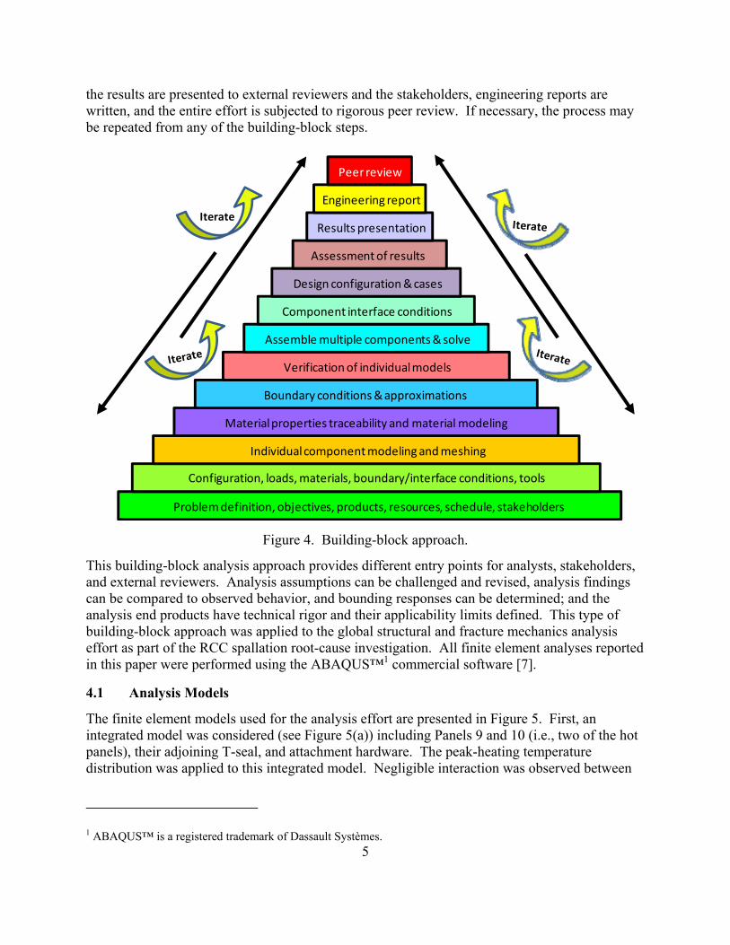
A building-block analysis approach begins with basic elements and builds in complexity in a systematic and progressive manner [2]. Such an approach permits each step in the process to be verified and its influence on the overall response determined. The hierarchy of the building-block approach is presented in Figure 4. First, the problem, objectives, products, resources, schedule, and stakeholders are defined. Second, the structural configuration, loads, materials, boundary/interface conditions, and tools to be used to solve to problem are identified. Next, analysis models, such as finite-element models of the individual components, are created. The material modeling procedure, boundary conditions, and other approximations are assigned to the individual component models, and the models are solved and verified for accuracy. The process at the individual component level is an iterative process that is repeated until the results can be verified by comparison to reference solutions or test data. Then, the individual component models are assembled, incorporating component interface conditions, different design configurations, and various load cases. The assembled models are solved, and the results are assessed. The process at the assembly level is also an iterative process that is repeated until confidence in the results can be demonstrated and advocated by the analysis team itself. Finally,

5

the results are presented to external reviewers and the stakeholders, engineering reports are written, and the entire effort is subjected to rigorous peer review. If necessary, the process may be repeated from any of the building-block steps.

Problem definition, objectives, products, resources, schedule, stakeholders

Configuration, loads, materials, boundary/interface conditions, tools

Individual component modeling and meshing

Material properties traceability and material modeling

Assemble multiple components & solve

Component interface conditions

Results presentation

Boundary conditions & approximations

Peer review

Verification of individual models

Engineering report

Design configuration & cases

Assessment of results

Iterate

Figure 4. Building-block approach.

This building-block analysis approach provides different entry points for analysts, stakeholders, and external reviewers. Analysis assumptions can be challenged and revised, analysis findings can be compared to observed behavior, and bounding responses can be determined; and the analysis end products have technical rigor and their applicability limits defined. This type of building-block approach was applied to the global structural and fracture mechanics analysis effort as part of the RCC spallation root-cause investigation. All finite element analyses reported in this paper were performed using the ABAQUS™1 commercial software [7].

4.1 Analysis Models

The finite element models used for the analysis effort are presented in Figure 5. First, an integrated model was considered (see Figure 5(a)) including Panels 9 and 10 (i.e., two of the hot panels), their adjoining T-seal, and attachment hardware. The peak-heating temperature distribution was applied to this integrated model. Negligible interaction was observed between

1 ABAQUS™ is a registered trademark of Dassault Systèmes.

6

Panel 10 and T-seal 10 for the peak-heating conditions. These results demonstrate that a single panel can be analyzed alone for the entry thermal conditions.

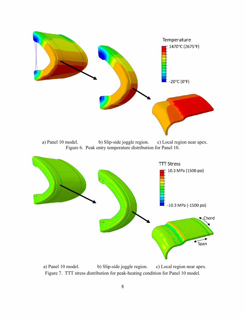
Next, the Panel 10 model shown in Figure 5(b) was considered because its slip-side joggle region experienced the highest entry temperature of the integrated model. The model had 3D elements all along the chord in the joggle regions and shell elements in the acreage regions. The peak entry temperature distribution shown in Figure 6 was applied to the model. The resulting through-the-thickness (TTT) stress distribution in the substrate is presented in Figure 7. (To show the TTT stresses clearly, the coating elements are removed in Figure 7.) As shown in Figure 7(c), an elevated stress value is observed all along the slip-side joggle in the local region near the panel apex (i.e., the hot region) and is nearly constant all along the chord direction (i.e., the gradient of stress in the chord direction is nearly zero). These results demonstrate that any slice perpendicular to the chord direction could be taken and used in a plane-strain analysis of the slip-side joggle [5].

Finally, the plane-strain model of the Panel 10 slip-side joggle region (shown in Figure 5(c)) was considered. For the stress analysis, the finite element model did not include craze cracks or defects. Because the temperatures in the local region near the panel apex are nearly constant (see Figure 6(c)), the maximum peak entry temperature was applied to the entire plane-strain model. The resulting TTT stress distribution in the substrate (the coating elements have been removed) is presented in Figure 8.

A failure criterion (or criteria) that is (or are) based on linear-elastic stress analysis results alone would suggest that wide-spread spallation would occur on many WLE panels on every mission, while the flight history shows that wide-spread spallation did not occur. Note that the observed spallation events shown in Figure 2 from flight history were limited to a single event at a single location on a single panel on each occurrence. However, the stress analysis results are used to indicate locations where potential subsurface defects may contribute to a spallation anomaly and prompted the following fracture mechanics analyses.

7

a) Integrated model.

b) Panel 10 model.

c) Plane-strain model. Figure 5. Analysis models.

8

a) Panel 10 model. b) Slip-side joggle region. c) Local region near apex. Figure 6. Peak entry temperature distribution for Panel 10.

a) Panel 10 model. b) Slip-side joggle region. c) Local region near apex. Figure 7. TTT stress distribution for peak-heating condition for Panel 10 model.

9

11.5 MPa (1664 psi)

‐2.7 MPa (‐387 psi)

TTT Stress

Figure 8. TTT stress distribution for peak-heating condition for plane-strain model.

5.0 Fracture Mechanics Analyses

The objective of the fracture mechanics analyses is to evaluate the defect driving forces, which are characterized by the strain energy release rates, and determine if defects can become unstable for each of the loading conditions.

The fracture mechanics analyses were performed using the plane-strain model. For the fracture mechanics analyses, subsurface defects were introduced at the maximum stress location (see Figure 8) and perpendicular to the maximum tensile TTT stress. Three types of defects were considered: interface defects (those along the coating-substrate interface), substrate defects (those completely within the substrate), and combined interface-substrate defects (those in both regions). Typical interface and substrate defects are presented schematically in Figure 9. In this paper, only interface and substrate defects are discussed.

a) Interface defect.

b) Substrate defect. Figure 9. Typical interface and substrate defects.

The finite element model and terminology are presented in Figure 10 (mesh is excluded for clarity). The panel acreage is to the left of the model. (Note that the orientation of Figure 10 is opposite to Figure 8. The orientation of Figure 10 is used in the remainder of the paper.) The

10

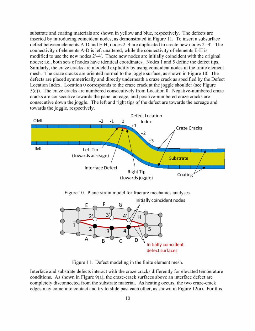
substrate and coating materials are shown in yellow and blue, respectively. The defects are inserted by introducing coincident nodes, as demonstrated in Figure 11. To insert a subsurface defect between elements A-D and E-H, nodes 2–4 are duplicated to create new nodes 2'–4'. The connectivity of elements A-D is left unaltered, while the connectivity of elements E-H is modified to use the new nodes 2'–4'. These new nodes are initially coincident with the original nodes; i.e., both sets of nodes have identical coordinates. Nodes 1 and 5 define the defect tips. Similarly, the craze cracks are modeled explicitly by using coincident nodes in the finite element mesh. The craze cracks are oriented normal to the joggle surface, as shown in Figure 10. The defects are placed symmetrically and directly underneath a craze crack as specified by the Defect Location Index. Location 0 corresponds to the craze crack at the joggle shoulder (see Figure 5(c)). The craze cracks are numbered consecutively from Location 0. Negative-numbered craze cracks are consecutive towards the panel acreage, and positive-numbered craze cracks are consecutive down the joggle. The left and right tips of the defect are towards the acreage and towards the joggle, respectively.

‐1 0+1

+2

+3

Interface Defect

Defect LocationIndex

Craze Cracks

OML

IML

Substrate

Coating

Left Tip(towards acreage)

Right Tip(towards joggle)

‐2

Figure 10. Plane-strain model for fracture mechanics analyses.

12 3 4 5

2' 3' 4'

A B C D

Initially coincident nodesE F G

H

Initially coincident defect surfaces

Figure 11. Defect modeling in the finite element mesh.

Interface and substrate defects interact with the craze cracks differently for elevated temperature conditions. As shown in Figure 9(a), the craze-crack surfaces above an interface defect are completely disconnected from the substrate material. As heating occurs, the two craze-crack edges may come into contact and try to slide past each other, as shown in Figure 12(a). For this

11

reason, friction is included in the finite element model to account for the craze-crack edge interaction. In contrast, as shown in Figure 9(b), the craze-crack surfaces above a substrate defect are connected to substrate material. When heating occurs, the two craze-crack edges may come into contact, but they are restrained from sliding past each other, as shown in Figure 12(b).

a) Interface defect with craze-crack edge interaction.

b) Substrate defect. Figure 12. Deflection of interface and substrate defects.

12

The capability of a structure with an embedded defect can be described using the total defect driving force GT calculated using fracture mechanics analyses; i.e., the problem is no longer a stress analysis problem. Once the defect driving force is computed, it can be compared to material toughness values for the different modes of fracture (Mode I, II, and/or their mixity for plane strain).

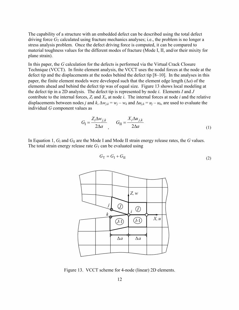
In this paper, the G calculation for the defects is performed via the Virtual Crack Closure Technique (VCCT). In finite element analysis, the VCCT uses the nodal forces at the node at the defect tip and the displacements at the nodes behind the defect tip [8–10]. In the analyses in this paper, the finite element models were developed such that the element edge length (a) of the elements ahead and behind the defect tip was of equal size. Figure 13 shows local modeling at the defect tip in a 2D analysis. The defect tip is represented by node i. Elements I and J contribute to the internal forces, Zi and Xi, at node i. The internal forces at node i and the relative displacements between nodes j and k, wj,k = wj – wk and uj,k = uj – uk, are used to evaluate the individual G component values as

a

wZG kji

2,

I, a

uXG

kji

2,

II (1)

In Equation 1, GI and GII are the Mode I and Mode II strain energy release rates, the G values. The total strain energy release rate GT can be evaluated using

IIIT GGG (2)

X, u

Z, w

a

J

J-1 I-1

j

ki I

a

Figure 13. VCCT scheme for 4-node (linear) 2D elements.

13

In this paper, a somewhat conservative comparison is made by comparing the total strain energy release rate GT to the Mode I fracture toughness GIc, which is the smallest of the fracture toughness values for the different modes. Unstable defect growth (i.e., defect is likely to grow in a catastrophic manner) may occur when GT is greater than or equal to GIc; i.e., GT/GIc ≥ 1.

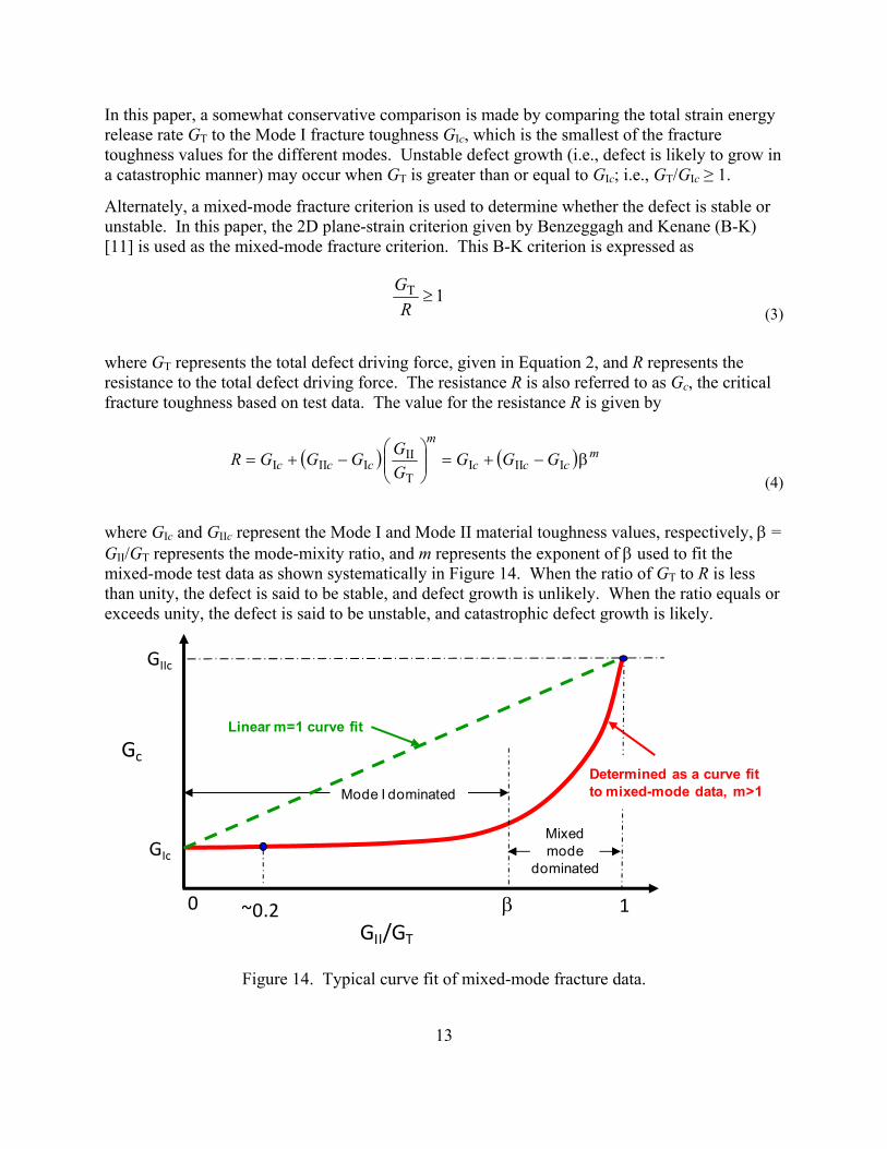
Alternately, a mixed-mode fracture criterion is used to determine whether the defect is stable or unstable. In this paper, the 2D plane-strain criterion given by Benzeggagh and Kenane (B-K) [11] is used as the mixed-mode fracture criterion. This B-K criterion is expressed as

1T

R

G

(3)

where GT represents the total defect driving force, given in Equation 2, and R represents the resistance to the total defect driving force. The resistance R is also referred to as Gc, the critical fracture toughness based on test data. The value for the resistance R is given by

IIIIT

IIIIII

mccc

m

ccc GGGG

GGGGR

(4)

where GIc and GIIc represent the Mode I and Mode II material toughness values, respectively, = GII/GT represents the mode-mixity ratio, and m represents the exponent of used to fit the mixed-mode test data as shown systematically in Figure 14. When the ratio of GT to R is less than unity, the defect is said to be stable, and defect growth is unlikely. When the ratio equals or exceeds unity, the defect is said to be unstable, and catastrophic defect growth is likely.

GII/GT

0 1

Gc

GIc

GIIc

~0.2

Mode I dominated

Linear m=1 curve fit

Mixedmode

dominated

Determined as a curve fit to mixed-mode data, m>1

Figure 14. Typical curve fit of mixed-mode fracture data.

14

For a mixed-mode response, the B-K resistance R given in Equation 4 is dependent on the value of the exponent m as indicated in Figure 14. This exponent is typically determined using a curve fit for mixed-mode fracture data obtained from material testing. For a value of m = 1, a linear response like the green dashed line in Figure 14 is obtained, which is a non-conservative criterion. Mixed-mode fracture tests of polymeric matrix composites show that the B-K criterion using m = 2 or 3 appears to fit mixed-mode fracture data accurately. A typical mixed-mode fracture criterion curve is shown as red in Figure 14. For mode-mixity ratios less than , the response is dominated by Mode I behavior.

Single cantilever beam and end-notch flexure test configurations were used in RCC fracture testing to determine GIc and GIIc. In the absence of further test data, a value of two was selected as the value of the exponent m. In addition, the B-basis fracture toughness values are used in evaluating Equation 4 as they provide a smaller value for R, which is conservative.

6.0 Results and Discussion

In this section, only representative results in terms of defect driving forces, the GT values, for entry peak heating and the on-orbit cold condition are presented. Both interface and substrate defects are considered. More detailed analyses and results can be found in References 1–6.

6.1 Interface Defects – Effect of Defect Location

Interface defects were studied by assuming a constant-length defect at different craze-crack locations. Both entry peak heating and the on-orbit cold condition were considered. The results for the normalized GT values are presented as the ratio GT/GIc. Values of GT/GIc less than unity indicate that the defect is stable and unlikely to grow catastrophically. Values greater than unity require further study. Such values could mean the defect is unstable and likely to grow catastrophically, or they could mean the mode of fracture is not Mode-I dominated. Hence, the total and individual component G values need to be calculated and assessed.

Entry Peak Heating. For entry peak heating, the craze-crack surfaces come into contact and slide past each other, as shown in Figure 15(a), and friction along the craze-crack edges influences the defect deformations. Figures 15(b) and 15(c) present the normalized GT values for two values of the coefficient of friction for various locations of the defect along the joggle. For each location, the interface defect is centered beneath the craze crack. Both the left and right tip normalized GT values are plotted as a function of the defect location. For = 0 (Figure 15(b)), the left tip values are considerably smaller than the right tip values for all defect locations considered. For both = 0 and = 0.4, the maximum normalized GT occurs at the shoulder of the joggle, Location 0. However, the normalized GT for = 0 is considerably higher than the normalized GT for = 0.4 indicating that the craze-crack edge interaction is an important variable to the defect driving force.

The individual mode G values were also examined. For both = 0 and = 0.4, the GI values are larger than the GII values. This result suggests that the defect opening for entry peak heating is dominated by Mode I.

15

a) Interface defect at craze-crack Location +1 and deformed configurations for interface defects at varying craze-crack locations (deformations scaled by a factor of 20).

b) Normalized GT for µ = 0.

c) Normalized GT for µ = 0.4. Figure 15. Normalized GT as a function of interface defect location – Entry peak heating.

16

On-Orbit Cold. For the on-orbit cold condition, the craze-crack surfaces displace away from each other, as shown in Figure 16(a), and the craze-crack edges do not interact and do not influence the defect deformations. Figure 16(b) presents the normalized GT values as a function of the interface defect location. The maximum normalized GT occurs in the acreage area (for the left tip at Locations –1 and 0). As the defect is moved into the joggle region, the normalized GT values decrease and reach a plateau. Both the left and right tips have nearly the same normalized GT values except at Location 0, where the left tip (towards the acreage) has the higher value. This difference in behavior at Location 0 is due to the geometry; at Location 0, half of the defect is in the acreage, and half is down the joggle curve.

The individual mode G values were also examined. The GII values are larger than the GI values, suggesting that the defect opening for on-orbit cold is dominated by Mode II and indicating that the comparison of GT to GIc in Figure 16(b) may be overly conservative.

a) Interface defect at craze-crack Location +1 and deformed configurations for interface defects at varying craze-crack locations (deformations scaled by a factor of 20).

b) Normalized GT. Figure 16. Normalized GT as a function of interface defect location – On-orbit cold.

17

6.2 Substrate Defects – Effect of Defect Length

The fracture mechanics response for substrate defects is examined by fixing the left tip of the defect at different acreage locations and then extending the defect along the joggle (i.e., changing the defect size or length). The notation ‘A→B’ is used in this paper to indicate that a subsurface defect exists between Location A and Location B. The left and right defect tips are located at Locations A and B, respectively, as illustrated in Figure 17(a).

Entry Peak Heating. To study “very long” substrate defects for entry peak heating, the left defect tip is placed at Location –2, and the location of the right defect tip is varied along the joggle up to Location +4. The fracture response is given in Figure 17(b) for the left tip and in Figure 17(c) for the right tip. The blue curves represent the total defect driving force, or GT, normalized by GIc, and the green dashed curves represent the resistance to the defect driving force, or R, evaluated using Equation 4 and normalized by GIc. For the initial case (i.e., case –2→0), both defect tips are stable. For longer defects (i.e., cases –2→+1 and –2→+2), the left tip is stable, but the right tip is unstable. For the case –2→+3, the normalized R at the right tip becomes larger than the normalized GT suggesting a return to a stable region. For the “very long” defect (i.e., case –2→+4), the left tip normalized GT exceeds the normalized R and hence the left tip becomes unstable.

a) Various defects with the left tip fixed at Location –2; case –2→+4 shown.

b) Left tip. c) Right tip. Figure 17. Fracture mechanics response for the left substrate defect tip fixed at Location –2.

18

7.0 Effect of Various Variables on the Defect Driving Force

As mentioned previously, there are many variables that contribute to the defect driving force, the GT value, for this application. Some of these variables are identified in Figure 18, and the effect of each of these variables is discussed qualitatively.

Defectinitiation site

Coating/substratetransition zone

Craze crackedge interaction

Stress‐freetemperature

Extent offiber bridging

Extent ofply convolutions

Defectgrowth model

3D effects

GT

GT

GT

Nonlinear‐ response GT

GTGT

Defect size

GT

Craze crackorientation

GT

Figure 18. Effect of various variables on defect driving force.

The effect of the variable in the green cloud (i.e., defect initiation site) was determined by studying the photomicrographs like the one shown in the center of this figure.

The effect of the variables in the orange clouds was determined [1 – 6] through finite element and fracture mechanics analyses like those presented in this paper. For the coating/substrate transition zone, the initial analyses assumed a sharp coating/substrate interface and yielded higher GT values. Because a sharp interface does not exist in reality, analyses were conducted using different size zones where the material properties were transitioned from substrate to coating, yielding lower GT values. For defect size, larger defects yield higher GT values. For 3D effects, part-through defects yield lower GT values than those computed using plane-strain analysis (i.e., simulating a through defect). These results demonstrate that plane strain is the bounding case. For the extent of fiber bridging, including fiber bridging yields lower GT values. For the extent of ply convolutions, including knuckles, voids, etc. yields higher GT values. For stress-free temperature, using a stress-free temperature that increases the T yields higher GT values. For craze-crack edge interaction, including friction in the analysis affects the results; high values for the coefficient of friction yield lower GT values, while simulating a smooth edge

19

using zero friction yields higher GT values. For craze-crack orientation, craze-cracks oriented normal to the joggle yield the lowest GT values.

The effect of the variables in the gray clouds (i.e., defect growth model and nonlinear stress-strain response) could not be quantified because enough RCC material was not available to perform comprehensive testing, in addition, testing at elevated temperatures is much more complex than at room temperature.

8.0 Concluding Remarks

The Space Shuttle wing-leading edge consists of panels that are made of reinforced carbon-carbon. On some panels that experience extreme heating, spallation of coating was observed in the slip-side joggle regions of the panels. Global structural and local fracture mechanics analyses were performed on these panels as a part of the root cause investigation of this coating spallation anomaly. The global structural analyses showed minimal interaction between adjacent panels and T-seals that bridge the gaps between the panels for entry thermal conditions. A bounding temperature distribution was applied to a representative panel, and the resulting stress distribution was examined. For this loading condition, the through-the-thickness normal stresses showed negligible variation in the chord direction and increased values in the vicinity of the slip-side joggle shoulder. As such, a representative span-wise slice on the panel was taken, and the cross section was analyzed using plane-strain analysis. In the plane-strain models, both interface and substrate defects were introduced. Various size defects were considered. Plane-strain finite element analyses were conducted for entry peak heating and on-orbit cold conditions. Defect driving forces in terms of the strain energy release rates were used to characterize the defects. This paper presents some of the fracture mechanics analyses and results.

Various parameters that affect the driving force of defects present in the Space Shuttle wing-leading-edge joggle regions have been identified. In this paper, the effects of defect initiation site and defect size were briefly presented. For the fracture mechanics analyses, interface, substrate, and combined defects were introduced into the 2D plane-strain finite element models of the slip-side joggle region. 3D analyses showed that the plane-strain case is the bounding case. The defect driving forces were computed using the Virtual Crack Closure Technique, and the Benzeggagh-Kenane mixed-mode fracture criterion was considered. Parameters that affect the defect driving force include effects of the coating/substrate transition region, fiber bridging, ply convolutions, stress-free temperature, and craze-crack orientation and edge interaction. The fracture mechanics analysis results were ultimately used to define tests and test methods and helped in understanding possible factors and scenarios that contribute to the RCC spallation anomaly.

20

9.0 References 1. Knight, N. F., Jr.; Raju, I. S.; Song, K.; and Phillips, D. R.: “Global and Fracture Mechanics

Analyses for the Space Shuttle Orbiter Wing-Leading-Edge Panels.” Proceedings of the International Conference on Computational and Experimental Engineering and Sciences ’10 Conference, March 29–April 1, 2010, Las Vegas, Nevada, Paper No. ICCES1020091224163.

2. Knight, N. F., Jr.; Raju, I. S.; Song, K.; and Phillips, D. R.: “Building-Block Analysis Strategy Applied to Space Shuttle Orbiter Wing-Leading-Edge Panels.” Proceedings of the International Conference on Computational and Experimental Engineering and Sciences ’10 Conference, March 29–April 1, 2010, Las Vegas, Nevada, Paper No. ICCES1020091224164.

3. Phillips, D. R.; Raju, I. S.; Knight, N. F., Jr.; and Song, K.: “Influence of Craze Cracks on Reinforced Carbon-Carbon Material Modeling.” Proceedings of the International Conference on Computational and Experimental Engineering and Sciences ’10 Conference, March 29–April 1, 2010, Las Vegas, Nevada, Paper No. ICCES1020091224165.

4. Knight, N. F., Jr.; Song, K.; Raju, I. S.; and Phillips, D. R.: “Fracture Response of a Composite Joggle Structure Including Ply Convolutions.” Proceedings of the International Conference on Computational and Experimental Engineering and Sciences ’10 Conference, March 29–April 1, 2010, Las Vegas, Nevada, Paper No. ICCES1020091224166.

5. Knight, N. F.; Jr., Song, K.; and Raju, I. S.: “Space Shuttle Orbiter Wing-Leading-Edge Panel Thermo-Mechanical Analysis for Entry Conditions.” Proceedings of the AIAA/ASME/ASCE/AHS/ASC 51st Structures, Structural Dynamics, and Materials Conference, April 12–15, 2010, Orlando, Florida, Paper No. AIAA-2010-2688.

6. Raju, I. S.; Phillips, D. R.; Knight, N. F., Jr.; and Song, K.: “Fracture Mechanics Analyses of Reinforced Carbon-Carbon Wing-Leading Edge Panels.” Proceedings of the AIAA/ASME/ASCE/AHS/ASC 51st Structures, Structural Dynamics, and Materials Conference, April 12–15, 2010, Orlando, Florida, Paper No. AIAA-2010-2689.

7. Anon.: ABAQUS Analysis User’s Manual: Volumes I – VI, Version 6.7. Dassault Systèmes Simulia Corp., Providence, Rhode Island, 2007.

8. Rybicki, E. F.; and Kanninen, M. F.: “A Finite Element Calculation of Stress Intensity Factors by a Modified Crack Closure Integral.” Engineering Fracture Mechanics, Vol. 9, No. 4, pp. 931–938, 1977.

9. Raju, I. S.: “Calculation of Strain-Energy Release Rates with Higher Order and Singular Finite Elements,.” Engineering Fracture Mechanics, Vol. 28, pp. 251–274, 1987.

10. Krueger, R.: “The Virtual Crack Closure Technique: History, Approach and Applications.” Applied Mechanics Reviews, Vol. 57, No. 2, pp. 109–143, 2004.

11. Benzeggagh, M. L.; and Kenane, M.: “Measurement of Mixed-Mode Delamination Fracture Toughness of Unidirectional Glass/Epoxy Composites with Mixed-Mode Bending Apparatus.” Composites Science and Technology, Vol. 56, No. 4, pp. 439-449, 1996.

REPORT DOCUMENTATION PAGEForm Approved

OMB No. 0704-0188

2. REPORT TYPE

Technical Memorandum 4. TITLE AND SUBTITLE

Fracture Mechanics Analyses of the Slip-Side Joggle Regions of Wing-Leading-Edge Panels

5a. CONTRACT NUMBER

6. AUTHOR(S)

Raju, Ivatury S.; Knight, Norman F., Jr.; Song, Kyongchan; Phillips, Dawn R.

7. PERFORMING ORGANIZATION NAME(S) AND ADDRESS(ES)

NASA Langley Research CenterHampton, VA 23681-2199

9. SPONSORING/MONITORING AGENCY NAME(S) AND ADDRESS(ES)

National Aeronautics and Space AdministrationWashington, DC 20546-0001

8. PERFORMING ORGANIZATION REPORT NUMBER

L-19965

10. SPONSOR/MONITOR'S ACRONYM(S)

NASA

13. SUPPLEMENTARY NOTESKeynote Lecture presented at the 9th YSESM Symposium in Trieste, Italy held during July 7-10, 2010.

12. DISTRIBUTION/AVAILABILITY STATEMENTUnclassified - UnlimitedSubject Category 39 Structural MechanicsAvailability: NASA CASI (443) 757-5802

19a. NAME OF RESPONSIBLE PERSON

STI Help Desk (email: help@sti.nasa.gov)

14. ABSTRACT

The Space Shuttle wing-leading edge consists of panels that are made of reinforced carbon-carbon. Coating spallation was observed near the slip-side region of the panels that experience extreme heating. To understand this phenomenon, a root-cause investigation was conducted. As part of that investigation, fracture mechanics analyses of the slip-side joggle regions of the hot panels were conducted. This paper presents an overview of the fracture mechanics analyses.

15. SUBJECT TERMS

Reinforced carbon-carbon, fracture mechanics; stress-free temperature; wing leading edge; joggle region; thermal loading; subsurface defects; finite element analysis; strain energy release rates

18. NUMBER OF PAGES

27

19b. TELEPHONE NUMBER (Include area code)

(443) 757-5802

a. REPORT

U

c. THIS PAGE

U

b. ABSTRACT

U

17. LIMITATION OF ABSTRACT

UU

Prescribed by ANSI Std. Z39.18Standard Form 298 (Rev. 8-98)

3. DATES COVERED (From - To)

5b. GRANT NUMBER

5c. PROGRAM ELEMENT NUMBER

5d. PROJECT NUMBER

5e. TASK NUMBER

5f. WORK UNIT NUMBER

869021.01.07.01.01

11. SPONSOR/MONITOR'S REPORT NUMBER(S)

NASA/TM-2011-216878

16. SECURITY CLASSIFICATION OF:

The public reporting burden for this collection of information is estimated to average 1 hour per response, including the time for reviewing instructions, searching existing data sources, gathering and maintaining the data needed, and completing and reviewing the collection of information. Send comments regarding this burden estimate or any other aspect of this collection of information, including suggestions for reducing this burden, to Department of Defense, Washington Headquarters Services, Directorate for Information Operations and Reports (0704-0188), 1215 Jefferson Davis Highway, Suite 1204, Arlington, VA 22202-4302. Respondents should be aware that notwithstanding any other provision of law, no person shall be subject to any penalty for failing to comply with a collection of information if it does not display a currently valid OMB control number.PLEASE DO NOT RETURN YOUR FORM TO THE ABOVE ADDRESS.

1. REPORT DATE (DD-MM-YYYY)

01 - 201101-