formally certified satisfiability solving by duck ki …
TRANSCRIPT

FORMALLY CERTIFIED SATISFIABILITY SOLVING
by
Duck Ki Oe
An Abstract
Of a thesis submitted in partial fulfillment of therequirements for the Doctor of Philosophy
degree in Computer Sciencein the Graduate College of
The University of Iowa
July 2012
Thesis Supervisor: Associate Professor Aaron D. Stump

1
ABSTRACT
Satisfiability (SAT) and satisfiability modulo theories (SMT) solvers are high-
performance automated propositional and first-order theorem provers, used as un-
derlying tools in many formal verification and artificial intelligence systems. Theo-
retic and engineering advancement of solver technologies improved the performance
of modern solvers; however, the increased complexity of those solvers calls for formal
verification of those tools themselves. This thesis discusses two methods to formally
certify SAT/SMT solvers. The first method is generating proofs from solvers and
certifying those proofs. Because new theories are constantly added to SMT solvers,
a flexible framework to safely add new inference rules is necessary. The proposal is
to use a meta-language called LFSC, which is based on Edinburgh Logical Frame-
work. SAT/SMT logics have been encoded in LFSC, and the encoding can be easily
and modularly extended for new logics. It is shown that an optimized LFSC checker
can certify SMT proofs efficiently. The second method is using a verified program-
ming language to implement a SAT solver and verify the code statically. Guru is a
pure functional programming language with support for dependent types and theorem
proving; Guru also allows for efficient code generation by means of resource typing. A
modern SAT solver, called versat, has been implemented and verified to be correct in
Guru. The performance of versat is shown to be comparable with that of the current
proof checking technology.
2
Abstract Approved:
Thesis Supervisor
Title and Department
Date

FORMALLY CERTIFIED SATISFIABILITY SOLVING
by
Duck Ki Oe
A thesis submitted in partial fulfillment of therequirements for the Doctor of Philosophy
degree in Computer Sciencein the Graduate College of
The University of Iowa
July 2012
Thesis Supervisor: Associate Professor Aaron D. Stump

Graduate CollegeThe University of Iowa
Iowa City, Iowa
CERTIFICATE OF APPROVAL
PH.D. THESIS
This is to certify that the Ph.D. thesis of
Duck Ki Oe
has been approved by the Examining Committee for the thesisrequirement for the Doctor of Philosophy degree in ComputerScience at the July 2012 graduation.
Thesis Committee:
Aaron Stump, Thesis Supervisor
Cesare Tinelli
Hantao Zhang
Alberto Segre
Gregory Landini
Natarajan Shankar

To Mi-Jeong and Claire and Monica
ii

ACKNOWLEDGEMENTS
First, and foremost, I would like to thank my advisor, Aaron Stump who has
always been supportive to me and encouraged me through out my doctoral study. It
was a great pleasure to learn from him and work with him. I was greatly fortunate that
I had him as my menor. I just followed his direction he led me to, never realizing what
I could have accomplish at the end of my study. Now, I am so proud of my graduate
work and very happy about my next position. Also, he really cares his student, and I
appreciate his support beyond teaching and advising. I thank Professor Cesare Tinelli
for being a wonderful role model. He has a very high standard for every aspect of
professorship from teaching to researching and writing papers. I learned many from
what he taught and also the way he did. I also would like to thank Sheryl Semler
and Catherine Till for always being kind and helpful. Finally, I thank my wife here
in Iowa and my family back in Korea for supporting and believing in me. Because
of their patience and sacrifice, I could do my favorite jobs in my life–studying and
raising children– all at the same time.
iii

TABLE OF CONTENTS
LIST OF TABLES . . . . . . . . . . . . . . . . . . . . . . . . . . . . . . . . . vi
LIST OF FIGURES . . . . . . . . . . . . . . . . . . . . . . . . . . . . . . . . vii
CHAPTER
1 INTRODUCTION . . . . . . . . . . . . . . . . . . . . . . . . . . . . . 1
1.1 Theorem Provers . . . . . . . . . . . . . . . . . . . . . . . . . . . 11.2 De Bruijn Criterion . . . . . . . . . . . . . . . . . . . . . . . . . 31.3 Correctness of Satisfiability Solvers . . . . . . . . . . . . . . . . . 41.4 Contributions . . . . . . . . . . . . . . . . . . . . . . . . . . . . 6
2 BACKGROUND: SATISFIABILITY SOLVING . . . . . . . . . . . . 8
2.1 The Classical DPLL Algorithm . . . . . . . . . . . . . . . . . . . 82.2 The Modern DPLL Algorithm . . . . . . . . . . . . . . . . . . . 102.3 SAT Solver Engineering . . . . . . . . . . . . . . . . . . . . . . . 132.4 Satisfiability Modulo Theories . . . . . . . . . . . . . . . . . . . 14
3 RELATED WORK . . . . . . . . . . . . . . . . . . . . . . . . . . . . 18
3.1 SAT Proof Checking . . . . . . . . . . . . . . . . . . . . . . . . . 183.1.1 Resolution-based Proof Formats . . . . . . . . . . . . . . 183.1.2 Linear Resolution-based Proof Formats . . . . . . . . . . 193.1.3 Reverse Unit Propagation . . . . . . . . . . . . . . . . . . 213.1.4 Trustworthiness of the Proof Checker . . . . . . . . . . . 23
3.2 SMT Proof Checking . . . . . . . . . . . . . . . . . . . . . . . . 253.3 Statically Verified SAT Solvers . . . . . . . . . . . . . . . . . . . 26
3.3.1 Verified SAT Solvers . . . . . . . . . . . . . . . . . . . . . 273.3.2 Limitations . . . . . . . . . . . . . . . . . . . . . . . . . . 28
4 SAT/SMT PROOF CHECKING USING A LOGICAL FRAMEWORK 31
4.1 The LFSC Language . . . . . . . . . . . . . . . . . . . . . . . . . 324.1.1 Notational Conventions . . . . . . . . . . . . . . . . . . . 344.1.2 Introducing LF with Side Conditions . . . . . . . . . . . . 354.1.3 Abstract Syntax and Informal Semantics . . . . . . . . . 37
4.2 Encoding Propositional Reasoning . . . . . . . . . . . . . . . . . 404.2.1 Encoding Propositional Resolution . . . . . . . . . . . . . 42
iv

4.2.2 Deferred Resolution . . . . . . . . . . . . . . . . . . . . . 464.3 Encoding Quantifier-Free Integer Difference Logic . . . . . . . . . 49
4.3.1 CNF Conversion . . . . . . . . . . . . . . . . . . . . . . . 494.3.2 Converting Theory Lemmas to Propositional Clauses . . . 524.3.3 Encoding Integer Difference Logic . . . . . . . . . . . . . 55
4.4 Results for QF IDL Proof Checking . . . . . . . . . . . . . . . . 564.5 Conclusion . . . . . . . . . . . . . . . . . . . . . . . . . . . . . . 59
5 VERIFYING MODERN SAT SOLVER USING DEPENDENT TYPES 60
5.1 The Guru Programming Language . . . . . . . . . . . . . . . . 605.1.1 The Guru Syntax . . . . . . . . . . . . . . . . . . . . . . 645.1.2 Verified Programming in Guru . . . . . . . . . . . . . . . 66
5.2 Formalizing Correct SAT Solvers . . . . . . . . . . . . . . . . . . 685.2.1 Representation of CNF Formulas . . . . . . . . . . . . . . 695.2.2 Deduction Rules . . . . . . . . . . . . . . . . . . . . . . . 705.2.3 The answer Type . . . . . . . . . . . . . . . . . . . . . . 725.2.4 Parser and Entry Point . . . . . . . . . . . . . . . . . . . 73
5.3 Implementation and Invariants . . . . . . . . . . . . . . . . . . . 745.3.1 Array-based Clauses and Invariants . . . . . . . . . . . . 755.3.2 Conflict Analysis with Optimized Resolution . . . . . . . 785.3.3 Summary of Implementation . . . . . . . . . . . . . . . . 84
5.4 Results: versat Performance . . . . . . . . . . . . . . . . . . . . 865.5 Discussion . . . . . . . . . . . . . . . . . . . . . . . . . . . . . . 895.6 Conclusion . . . . . . . . . . . . . . . . . . . . . . . . . . . . . . 91
APPENDIX . . . . . . . . . . . . . . . . . . . . . . . . . . . . . . . . . . . . . 92
A APPENDICES FOR LFSC ENCODINGS . . . . . . . . . . . . . . . . 92
A.1 Typing Rules of LFSC . . . . . . . . . . . . . . . . . . . . . . . . 92A.2 Formal Semantics of Side Condition Programs . . . . . . . . . . 95A.3 Helper Code for Resolution . . . . . . . . . . . . . . . . . . . . . 96A.4 Small Example Proof . . . . . . . . . . . . . . . . . . . . . . . . 96
B APPENDICES FOR VERSAT . . . . . . . . . . . . . . . . . . . . . . . 101
B.1 Formal Syntax of Guru . . . . . . . . . . . . . . . . . . . . . . . 101B.2 Helper Code in the Guru Standard Library . . . . . . . . . . . . 103
REFERENCES . . . . . . . . . . . . . . . . . . . . . . . . . . . . . . . . . . . 105
v

LIST OF TABLES
Table
4.1 Summary of results for QF IDL . . . . . . . . . . . . . . . . . . . . . . . 57
5.1 Summary of variables used in ResState . . . . . . . . . . . . . . . . . . 84
5.2 Results for the certified track benchmarks of the SAT competition 2007 . 88
vi
LIST OF FIGURES
Figure
2.1 The classical DPLL algorithm . . . . . . . . . . . . . . . . . . . . . . . . 9
2.2 The modern DPLL algorithm . . . . . . . . . . . . . . . . . . . . . . . . 10
4.1 Main syntactical categories of LFSC . . . . . . . . . . . . . . . . . . . . 37
4.2 Definition of propositional clauses in LFSC concrete syntax . . . . . . . . 42
4.3 Propositional resolution calculus in LFSC concrete syntax . . . . . . . . 43
4.4 An example refutation and its LFSC encoding . . . . . . . . . . . . . . . 45
4.5 New constructors for the clause type and rules for deferred resolution . . 47
4.6 Pseudo-code for side condition function used by the S rule . . . . . . . . 47
4.7 Sample CNF conversion rules for partial clauses . . . . . . . . . . . . . . 51
4.8 LFSC proof rule for rename transformation . . . . . . . . . . . . . . . . . 52
4.9 The literal rule for partial clauses and its LFSC encoding . . . . . . . . . 53
4.10 Assumption rules for theory lemmas in LFSC concrete syntax . . . . . . 53
4.11 Sample QF IDL rules and LFSC encodings . . . . . . . . . . . . . . . . . 55
4.12 LFSC encoding of the idl contra rule . . . . . . . . . . . . . . . . . . . . 55
4.13 Solve-only times versus proof checking times for QF IDL . . . . . . . . . 59
5.1 Sample Guru definitions . . . . . . . . . . . . . . . . . . . . . . . . . . . 65
5.2 Encoding of the inference system (pf) and its helper functions . . . . . . 71
5.3 Definition of the answer type . . . . . . . . . . . . . . . . . . . . . . . . 72
5.4 Definition of the array-based clauses and invariants (aclause) . . . . . . 75
vii

5.5 Conflict analysis — a linear sequence of resolutions . . . . . . . . . . . . 78
5.6 Naive implementation of resolution . . . . . . . . . . . . . . . . . . . . . 79
5.7 Avoiding duplicated literals using a look-up table . . . . . . . . . . . . . 80
5.8 Data structure for optimized resolution . . . . . . . . . . . . . . . . . . . 80
5.9 Definition of conflict analysis state (ResState) . . . . . . . . . . . . . . . 83
5.10 Correctness theorem for table-clearing code . . . . . . . . . . . . . . . . 85
A.1 Bidirectional typing rules and context rules for LFSC . . . . . . . . . . . 92
A.2 Typing Rules for Code Terms . . . . . . . . . . . . . . . . . . . . . . . . 94
A.3 Operational semantics of side condition programs . . . . . . . . . . . . . 95
A.4 Variable and literal comparison . . . . . . . . . . . . . . . . . . . . . . . 97
A.5 Operations on clauses . . . . . . . . . . . . . . . . . . . . . . . . . . . . 98
A.6 A small QF IDL proof . . . . . . . . . . . . . . . . . . . . . . . . . . . . 99
B.1 Syntax for Guru terms (t) and types (T ) . . . . . . . . . . . . . . . . . 102
B.2 Syntax for Guru Formulas (F ) . . . . . . . . . . . . . . . . . . . . . . . 102
B.3 Syntax for Guru commands . . . . . . . . . . . . . . . . . . . . . . . . . 102
viii
1
CHAPTER 1
INTRODUCTION
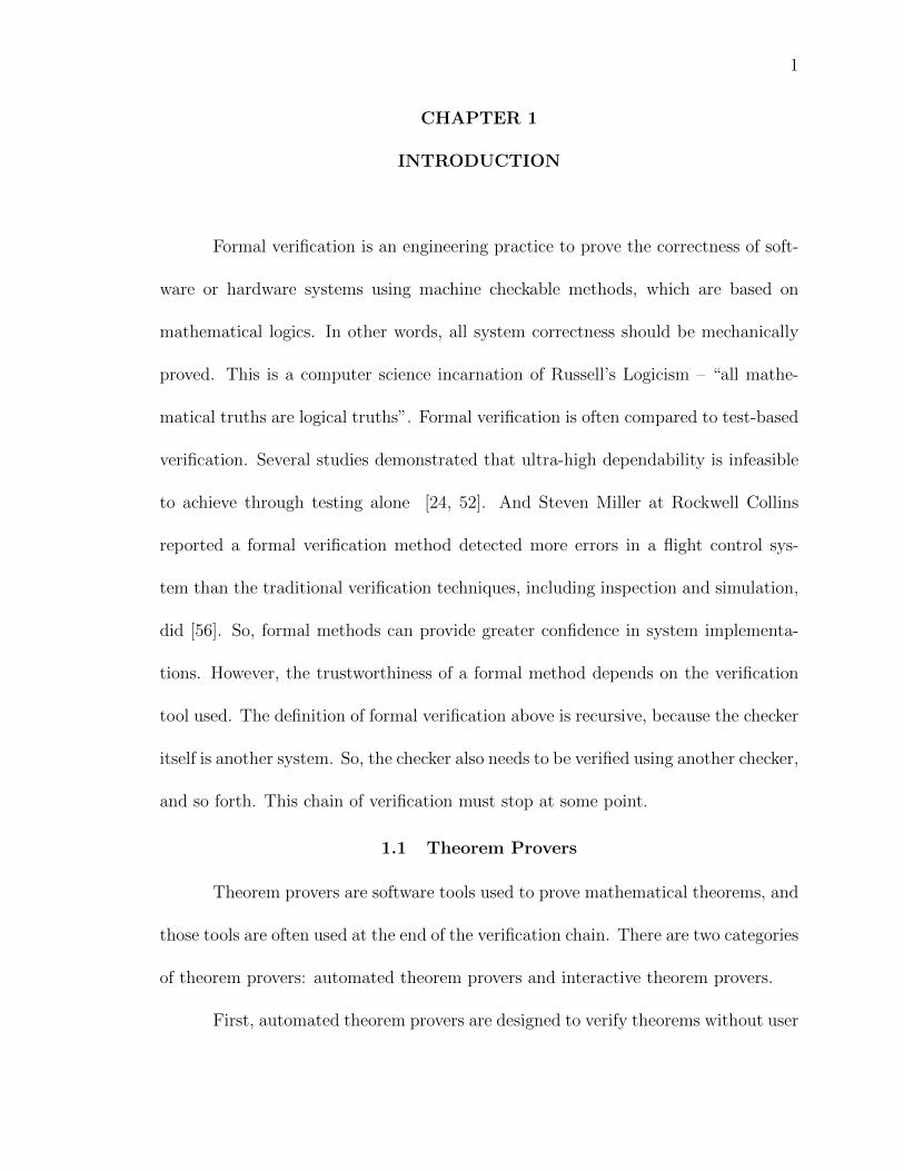
Formal verification is an engineering practice to prove the correctness of soft-
ware or hardware systems using machine checkable methods, which are based on
mathematical logics. In other words, all system correctness should be mechanically
proved. This is a computer science incarnation of Russell’s Logicism – “all mathe-
matical truths are logical truths”. Formal verification is often compared to test-based
verification. Several studies demonstrated that ultra-high dependability is infeasible
to achieve through testing alone [24, 52]. And Steven Miller at Rockwell Collins
reported a formal verification method detected more errors in a flight control sys-
tem than the traditional verification techniques, including inspection and simulation,
did [56]. So, formal methods can provide greater confidence in system implementa-
tions. However, the trustworthiness of a formal method depends on the verification
tool used. The definition of formal verification above is recursive, because the checker
itself is another system. So, the checker also needs to be verified using another checker,
and so forth. This chain of verification must stop at some point.
1.1 Theorem Provers
Theorem provers are software tools used to prove mathematical theorems, and
those tools are often used at the end of the verification chain. There are two categories
of theorem provers: automated theorem provers and interactive theorem provers.
First, automated theorem provers are designed to verify theorems without user

2
intervention. They are often based on traditional logics, like propositional logic or
first order (predicate) logic. Propositional logic is decidable and its decision proce-
dures have been studied under the name of the satisfiability (SAT) problem. SAT
solvers search for an interpretation of the propositional symbols that makes the given
formula true and report whether or not there exists such an interpretation. Because
the validity of a formula can also be deduced from the unsatisfiability of its negation,
a SAT solver can be used as a propositional theorem prover. For first order logics,
although they are generally undecidable, there are numerous approaches for automat-
ing first order theorem proving. Some provers, including Prover9 [54], search for a
proof of a given theorem, although that procedure may not terminate. These provers
allow users to define their own axioms. Other provers try to restrict the language and
find an efficiently decidable subset of first-order logics. For example, ground formulas
with linear/real integer arithmetics are decidable. Thus, theorem proving in such
logics can be fully automated. The field of satisfiability modulo theories (SMT) [13]
represents such efforts to define decidable fragment of first order logics and develop
efficient decision procedures. SMT is a first order logic version of the satisfiability
problem. A SMT logic is a first order logic with equality and a combination of certain
theories such as linear integer/real arithmetic, bit-vectors, and arrays. SMT solvers
are based on the theory that independent decision procedures for individual theories
can collectively build a decision procedure for the whole logic with those theories
combined [60]. Thus, SMT solvers can be easily extended with new theories. The
performance of SAT/SMT solvers has been improved greatly in the last decade, and
3
they are critical components of verification methods like model checking [25, 45] and
symbolic execution [48].
Second, interactive theorem provers are essentially proof checkers of inductive
calculi. They are designed to prove properties of mathematical functions and can also
be used to verify software and hardware systems. Interactive theorem provers are also
called proof assistants, because they provide some level of automation to help with
proof construction. Proof construction is interactive because the underlying logics
are undecidable and inductive proofs usually require human’s intervention. Although
those theorem provers are equipped with some automated proof generation features
(called “tactics”), the human creativity seems to be the key of theorem proving.
Recent works showed that interactive theorem provers can be used to verify important
properties of complex software systems. CompCert is an optimizing compiler for a
subset of the C programming language, for which semantics preservation has been
proved in the Coq theorem prover [50, 20]. The seL4 microkernel verification effort
uses the Isabelle theorem prover to prove that the microkernel implementation in
C and assembly follows a high-level non-deterministic model expressing the desired
system properties [47].
1.2 De Bruijn Criterion
Some theorem provers were constructed in a principled way to increase the
trustworthiness of the provers. The De Bruijn criterion characterizes verification
systems producing proof objects that can be independently checked using a simple
checker[11]. The original Automath system, invented by De Bruijn, in the late 60’s

4
was a proof checker and had a small kernel. The kernel essentially implements a proof
checker of the underlying logic. This piece of software is often called the trusted core
or trusted base, and it is the ultimate authority on logical truths upon which various
theories and theorems can be expressed and proved. If the core is small enough, it
can be peer reviewed and verified manually by inspection. The Automath systems
are based on the idea that type checking is equivalent to proof checking [39]. Pop-
ular systems following the same idea include LF [46], Twelf [8], Nuprl [26], Coq [2],
and Agda [1]. Also, there is another important method that meets the De Bruijn
criterion, called the LCF approach. Robin Milner implemented his Logic for Com-
putable Functions (LCF) [44]. LCF is well known for its use of a new programing
language, called ML (for “meta language”), to define the logic and implement tac-
tics altogether. In LCF, theorems are objects (of the thm type), and those theorems
can be built only by applying certain functions, which correspond to the proof rules.
Thus, even though tactics are implemented in the same language and can be arbi-
trarily complex, they cannot harm the soundness of the whole system, and thus are
outside of the trusted core. The HOL [3] and Isabelle [4] theorem provers are based
on the LCF approach [43].
1.3 Correctness of Satisfiability Solvers
Unlike the LCF and its descendants, mainstream SAT/SMT solvers are not
built on small foundations. Instead, they are tested against each other over a large set
of formulas. The usefulness of a SAT/SMT solver depends on its sheer performance
solving large formulas. So, they are implemented in conventional programming lan-

5
guages like C++ with emphasis on performance. Although the correctness of solver
algorithms is proved on paper, the implementations are mostly unverified. Popu-
lar SAT solvers are relatively small in size (about 2500 lines of C++) and believed
to be correct. However, the internal engineering of those SAT solvers is very so-
phisticated, and it is not practical to verify the code just by inspection. Indeed,
Brummayer discovered incorrect answers from the top solvers which participated in
the SAT competition 2006 and 2008 [23]. Thus, formal verification techniques for
SAT/SMT solvers themselves are highly desired. Currently, there are two distinct
approaches for verified SAT/SMT solving. One is to verify the certificates generated
from solvers. The other is to verify the code of solvers.
Proof checking. The advantages of certificate generation are: 1) it requires min-
imal changes to existing solvers, 2) certificates can be used for other purposes such
as counterexample presentation and interpolant generation [66]. The disadvantage
of proof generation is time and space costs for generating and checking certificates.
For satisfiable formulas, models can be generated as certificates and checked by a
simple trusted evaluator. For unsatisfiable formulas, certificates are in the form of
refutational proof. SAT is well known as the first NP-hard problem identified [27].
Instances of the SAT problem have small positive certificates (models), but not neces-
sarily small negative certificates (proofs). So, the size of proofs and the performance
of proof checking can be an issue in adopting a certificate-based verification method.
On the other hand, first order formulas do not have simple certificates in general.
However, quantifier-free formulas with a limited use of function symbols may have
6
simple models, which can then be checked.
Verifying the code. Statically verified solvers can solve and certify formula with-
out a proof checking overhead. However, modern SAT solvers, setting aside SMT
solvers, are quite sophisticated software, thus it is challenging to verify their code.
The usual approach is to implement the solver in a interactive theorem prover and
prove the answer is always correct according to the definition of satisfiability.
1.4 Contributions
As discussed in Section 1.3, proof checking and verifying the solver’s code are
two main approches for formally certified satisfiability solving. This dissertation re-
ports on the two novel implementations: 1) a SAT/SMT proof checking system using a
logical framework; 2) a statically verified SAT solver in a dependently typed program-
ming language. Our proof checking method uses a logical framework called LFSC,
which is distinguished from other solutions. LFSC is designed and implemented by
my advisor, Aaron Stump and his former students. This dissertation suggests an ef-
ficient proof certification method using the LFSC language and the optimized LFSC
type checker. Aaron Stump, Andrew Reynolds and I worked together on the encod-
ing of SAT reasoning, namely the efficient resolution rule (discussed in Section 4.2).
I encoded the QF IDL SMT logic (discussed in Section 4.3). I also implemented a
SAT/SMT solver, called clsat, which produces proofs in the proposed format. 1
1 Although clsat started as a class project with other students at Washington Universityin St. Louis, I have rewritten most of the code, except for the parser code for reading SMTformula files, which is mainly written by Timothy Simpson.

7
Our statically verified SAT solver, called versat, implements modern SAT solver
features and low-level optimizations. versat is written in the Guru programming
language, which is a functional programming language with support for dependent
types. The Guru language and the compiler have been designed and implemented
by Aaron Stump with his former students. I wrote the SAT-specific code/proofs of
versat. Aaron Stump, Corey Oliver, and Kevin Clancy helped me to prove theo-
rems about general data structures like machine words, lists and vectors. Because
SAT/SMT solvers have gained its popularity for their performance and scalability to
solve large formulas, the performance of certified SAT/SMT solvers are crucial for
any practical applications. Thus, the focus of our research was on the performance
of our implementations.
This dissertation is organized as following: Chapter 2 reviews the basics of
SAT/SMT solver algorithms and features. Chapter 3 surveys the related work on
certifying SAT/SMT solvers. Chapter 4 is based on our previously published work-
shop papers [74, 64] and recently accepted journal paper, and it reports on our proof
checking method. Chapter 5 extends our recently published conference paper [65]
and reports on the verified SAT solver we implemented.
8
CHAPTER 2
BACKGROUND: SATISFIABILITY SOLVING
Mainstream SAT solvers, including the state-of-the-art SAT solvers MiniSAT [33]
and PicoSAT [19], are based on the Davis-Putnam-Logemann-Loveland (DPLL) al-
gorithm [30]. Also most SMT solvers use SAT solvers internally as propositional
reasoning engines, which interact with the decision procedures for theories.
2.1 The Classical DPLL Algorithm
Figure 2.1 shows the classical DPLL algorithm. The input formula Φ is in
conjunctive normal form (CNF), and the partial model M is represented as a set of
consistent literals (never having both v and ¬v), where the polarity of each literal
means the truth-value assigned to the variable. Initially, M is empty and the DPLL
function returns true if the formula is satisfiable, or false, otherwise. The variable
M is a partial model, represented as a set of literals. A clause with only one literal
is called unit. A clause is also called unit when it has only one literal that is not
assigned in the partial model M and all the other literals are false under M. The unit-
propagation procedure repeatedly extends the current partial model M by adding the
literal from a unit clause. The existence of the empty clause under M means the
formula is falsified by M. So, when the algorithm finds a contradiction under M ∪ d
—DPLL(Φ, M∪ d) returns false—, the algorithm backtracks past the last literal and
tries the other polarity d. If DPLL returns false on both M ∪ d and M ∪ d, then any
model containing M cannot satisfy the formula. Especially, if DPLL returns false and

9
function DPLL(Φ,M)for every unit clause l in Φ under M unit-propagation
M := M ∪ l;if a clause in Φ is false under M then conflict
return false;if M contains all variables in Φ then
return true;d := choose-literal(Φ,M);return DPLL(Φ,M ∪ d) or DPLL(Φ,M ∪ d);
Figure 2.1. The classical DPLL algorithm (simplified). Φ is the input formula, andM is a partial model. The choose-literal function returns an arbitrary literal from Φthat is not defined under M. l means the opposite polarity of l.
M is empty, the formula is unsatisfiable. On the other hand, if Φ has no conflicts and
M is a complete model, then Φ is satisfiable. The algorithm in Figure 2.1 does not
return the found model, though it can be easily modified to return the model M. The
classical DPLL algorithm is fairly straightforward. Below is an informal analysis of
the algorithm:
Soundness. DPLL returns true only if the model M contains all the variables in Φ
and there is no conflict. That means the formula can be fully evaluated under the
model and the truth-value of the formula is true. Also, the function returns false
only if the formula has no model. This can be proved by induction on the number
of variables in the formula unassigned under M. Thus, the algorithm returns correct
answers.
Completeness. The number of variables in the formula is finite. Each recursive
call reduces the number of unassigned variable by one, and the function returns when

10
function Modern-DPLL(Φ)M := ∅ partial modellevel := 0repeat
for every unit clause l in Φ under M unit-propagationM := M ∪ l;
if a clause in Φ is false under M thenif level = 0 then
return false;c := analyze() conflict analysislevel := calc-level(c)d := uip-lit(c)M := backtrack(M, level)M := M ∪ dΦ := Φ ∧ c clause learning
elseif M contains all variables in Φ then
return true;level := level + 1d := choose-literal(Φ,M);M := M ∪ d
Figure 2.2. The modern DPLL algorithm. The analyze function deduces a clausefrom Φ as a lemma, and the calc-level function calculates the new decision level tobacktrack. And the uip-lit function returns the only literal in c that assigned on andafter the last decision point.
all variables are assigned. Thus, the depth of recursive call is limited by the number
of variables. Therefore, the algorithm is terminating.
2.2 The Modern DPLL Algorithm
Figure 2.2 shows the modern version of the DPLL algorithm. It has a top-level
loop (repeat), instead of a primitive recursion as in the classical algorithm, which
makes the execution flow more complex. The variable level keeps track of how many
chosen literals are in the current model M at any given time. Every time a literal is

11
chosen (choose-literal) and added to the model M, the level gets increased by one. The
level value corresponds to the recursion depth in the classical version. The biggest
difference from the classical DPLL is how conflicts are handled.
Conflict Analysis. Under the current partial assignment, if a clause is falsified,
the analyze function deduces a new clause, called a conflict clause, from the existing
set of clauses, with a very small cost of performance [70]. Conflict analysis performs
a series of resolutions, where the (propositional) resolution rule is:
x ∨ C ¬x ∨DC ∨D resolution
During the analysis, the SAT solver repeatedly resolves out recently assigned literals,
though it can add more literals. The idea is that the SAT solver wants to compute
a new clause with fewer literals that are assigned recently. This process stops when
it deduce a clause with only one literal assigned at the current level, which is called
the first unique implication point (UIP) literal. Sometimes, a conflict clause may
imply that the current conflict stems from a far earlier branching choice, instead of
the last choice. Then, the new clause may instruct the solver to backtrack multiple
choices (backjumping), so more search space is pruned. Also, this part of the SAT
solver is the main target of soundness verification, because it is where deduction is
performed. Compared to the fact that the classical DPLL performs purely semantic
exploration, the modern DPLL is a combination of semantic exploration and syntactic
manipulation applying deduction rules.

12
Backjumping. Once a conflict clause c is derived, the new level is calculated from
the clause. The calc-level function compares the levels at which variables in the
conflict clause are assigned, and returns the second highest level. (The highest level
is always the current level, because of the UIP literal.) In fact, the algorithm implicitly
records the level at which each variable is assigned. Then, the current level is updated
and the backtrack function removes literals that are assigned above the new level. This
is called backjumping, because the level may decrease by more than one, depending
on the conflict clause. Also, because the conflict clause is always unit under the new
M, the UIP literal d is assigned.
Clause Learning. Finally, and also optionally, the conflict clauses can be stored in
the clause database to prune out even more search space later on. However, it is also
possible that the increasing size of the clause database slows down unit propagation.
Thus, clause learning is used with heuristics about what kind of clauses should be
added, and when to drop them.
Correctness. Due to the dynamic nature of the modern DPLL algorithm, it is
much more complicated to analyze the correctness of the algorithm. Nieuwenhuis
et al. formalized the DPLL procedure as a state transition system, called Abstract
DPLL, and showed that the abstract system is sound and complete [62, 61]. Abstract
DPLL captures the core state of a SAT solver and represents it as a pair of a partial
assignment sequence and the set of clauses. It also defines transition rules that reflect
the operations performed in SAT solvers. Using the abstract DPLL framework, it is

13
easy to see that the classical and modern algorithms follow the abstract system and
thus are correct.
2.3 SAT Solver Engineering
Some important SAT solver features are abstracted away in the algorithms
above.
Efficient Unit Propagation. Unit-propagation, also called Boolean Constraint
Propagation (BCP), is a procedure to assign the truth values for certain literals when
each of those literals is the only literal in a clause left unassigned. So, there is only
one choice of assignment to make that clause true. To perform unit-propagation
efficiently, SAT solvers need to index the occurrences of each literal. The common
technique is using the two-literal watch lists where only two literals of each clause are
indexed [58, 83, 82].
Decision Heuristics. Deciding which variable to assign at the given point is an
important heuristic of SAT solvers. SAT solvers use some variations of the VSIDS (for
Variable State Independent Decaying Sum) method [58]. VSIDS maintains a score
board of all the variables, showing how active they are in the current search branch.
The definition of activity is different from solver to solver. The usual heuristic is to
decide the most active variable, but the activity value decays to emphasize recent
activities.

14
Restarts. The usual decision heuristics try to stay in the same search branch, which
can be very deep and not promising. The restarts technique [42] monitors the solver’s
activity and, if the solver is spending too much time in a particular search branch, it
forces the solver to backtrack all the way up to the search root. This helps solvers
escape out of a deep branch and try another branch, which might lead to an early
conclusion. This is also a heuristic and its utility depends on the characteristics of
the formula.
Conflict Clause Minimization. This is an extension of conflict analysis and tries
to minimize the size of the conflict clause by applying the self-subsumption rule [71].
When the conflict clause looks like x∨C ∨D and there is another clause like ¬x∨C,
x can be dropped from the conflict clause:
x ∨ C ∨D ¬x ∨ CC ∨D self subsumption
A typical SAT solver has a log of clauses that may allow self-subsumptions. But,
different solvers have different heuristics for how much time they will spend searching
for such clauses. If successful, this search time can be rewarded with a shorter conflict
clause. Shorter clauses are stronger and can prune even more search space.
2.4 Satisfiability Modulo Theories
Satisfiability Modulo Theories (SMT) refers to the satisfiability of a first order
formula in a theory or a combination of theories [13]. Many applications of formal
methods translate verification conditions into first-order logic formulas with some
theory, which fixes the interpretations of certain predicates and function symbols; for

15
example, inequalities and arithmetic operators. General first-order theorem proving
with additional axioms is not realistic for large formulas. Instead, using specialized
reasoning methods for the specific theory turns out to be a more successful alternative.
Many theories of integers and real numbers are in fact decidable and they have efficient
decision procedures. And more and more decision procedures have been discovered
for other data types such as arrays, strings and bit vectors. Nelson and Oppen showed
that decision procedures for individual theories can cooperate to solve formulas in the
combined theory [60]. This makes it easier to design SMT solvers supporting logics
with multiple theories combined.
A common SMT solver design is based on a SAT solver integrated with a
decision procedure for a first order theory (or “theory solver”) [35]. The SAT and
theory solvers are clearly separated inside the SMT solver, and interact with each
other in the following way:
1. The internal SAT solver solves the formula as if atomic formulas are just propo-
sitional variables, ignoring any meaning of those atomic formulas. For example,
a formula, (0 < x) ∧ (x < 0) is treated as though it is P ∧Q.
2. If the SAT solver reports unsatisfiable, the original formula is reported un-
satisfiable. That is because the formula is refutable only using propositional
deduction rules, without any theory axioms. On the other hand, if the SAT
solver reports satisfiable, then there will be a model, which includes (possibly
negated) atomic formulas. Because the SAT solver did not consider the meaning
of the atomic formulas, the model can be inconsistent. For the same example
16
above, 0 < x, x < 0 can be a model reported from the SAT solver, which
happens to be inconsistent with respect to the theory of integer/real numbers.
3. This model has to be checked against the desired theory. The theory solver
tries to find an inconsistency among theory formulas in the model. If there is no
inconsistency, the original formula is reported SAT. If there is an inconsistency
among some of the theory formulas, φ1, φ2, · · ·φn (where φi are atomic formulas
or negated ones), the theory solver gives the SAT solver a new clause, ¬φ1 ∨
¬φ2 ∨ · · · ∨ ¬φn (called a “theory lemma”). Theory lemmas are necessary to
eliminate the inconsistent models found by the SAT solver. From the SAT
solver’s point of view, theory lemmas are just new constraints to satisfy. For
the example model above, the theory lemma will be 0 6< x ∨ x 6< 0. And the
solver goes back to the step (1) and repeats.
This approach is called lazy theory reasoning, because the theory solver pas-
sively reacts to the SAT solver. Popular SMT solvers, including including CVC3 [15]
and Z3 [32], are based on this approach.
Satisfiability certificates are usually semantic models of formulas. For SAT
formulas, a certificate of satisfiability is a set of truth-value assignments to the propo-
sition variables in the given formula. For SMT formulas, a satisfiability certificate is a
model for the constant and function symbols of the formula. Mainstream SAT/SMT
solvers have support for producing models for satisfiable formulas. For SAT, models
can be efficiently verified by a simple trusted evaluator. In fact, the SAT compe-
tition requires all participants to generate models for satisfiable formulas [5]. For
17
SMT, describing and checking models can be complicated, due to infinite domains
and function interpretations. However, the SMT-LIB initiative is trying to define a
standard model format as well as the SMT formula format and standard logics [14].
Using models generated from solvers is also a common practice. When verification
conditions of a software and hardware system are formulated in the propositional
logic or a first order logic, a SAT/SMT solver is used to check the conditions. If the
solver answers “yes” (satisfiable), it means the condition is not valid and the model
generated from the solver is a counterexample.
18
CHAPTER 3
RELATED WORK
3.1 SAT Proof Checking
The SAT competition is a bi-yearly event where the best SAT solvers compete
against each other [5]. As a part of the competition, there is a separate category, called
certified UNSAT, where solvers are required to generate proofs of unsatisfiability. For
the certified track, several proof formats have been proposed over time. The RES
and RUP formats are the two recent standard formats accepted at the competition,
and the TraceCheck format is gaining popularity. In this section, I discuss SAT/SMT
proof systems and static verification of SAT solvers.
3.1.1 Resolution-based Proof Formats
The resolution rule is refutation complete by itself. And resolution is used
during clause learning in state-of-the-art SAT and solvers [84]. The resolution proof
format (RES), used at the SAT competition 2005, is based directly on the resolution
rule [37]. A RES proof is a sequence of resolution steps. Each resolution step records
two premises to resolve, the pivot literal, and the resolvent. Each step is given a
reference number and the number can be used to mention the clause proved at that
step. For an input formula with n clauses, the clauses in the input formula are named
from 1 to n, and reference numbers in its proof start from n + 1. Those reference
numbers are used to record the premises of each resolution step. In every proof, the
last step is supposed to prove the empty clause.

19
For example, consider this CNF formula, (p1 ∨ p2) ∧ (p1 ∨ ¬p2) ∧ (¬p1 ∨ p2) ∧
(¬p1 ∨ ¬p2). And an example refutation proof is below.
5 p1 1 2 p26 ¬p1 3 4 p27 · 5 6 p1
In this proof, the four input clauses are implicitly numbered from 1 through 4. Let
Ci be the clause numbered i. The first line gives a singleton clause p1 the number 5
and justifies the deduction of that clause by resolving the clause C1 and C2 over the
literal p2. Similarly, the clause C6, which is ¬p1, is proved. Finally, the empty clause
(·) is proved by resolving the clauses C5 and C6.
The RES format is simple and easy to understand. Also, because proofs
contain both the clauses to prove and their justifications, it is easy to find bugs in
the solver and the checker. However, for the same reason, the sizes of proofs can be
very large. So, to shrink the sizes of proofs, an alternative format, called resolution
proof trace (RPT), was proposed, where the resolvents (clauses) are omitted.
The advantage of the RES format is that checking a RES proof does not take
additional memory space beside the proof itself. There is no need to compute and
store anything additionally. However, the RES/RPT formats are considered too fine-
grained and hard to instrument existing solvers to generate proofs. How to generate
resolution proofs from SAT solvers is discussed in [76].
3.1.2 Linear Resolution-based Proof Formats
Most modern SAT solvers implements a feature called conflict analysis to de-
duce a new clause, called conflict clause, as a lemma. It is well known that conflict
analysis can be represented as a series of (linear) resolution steps [41, 85, 17]. Res-
20
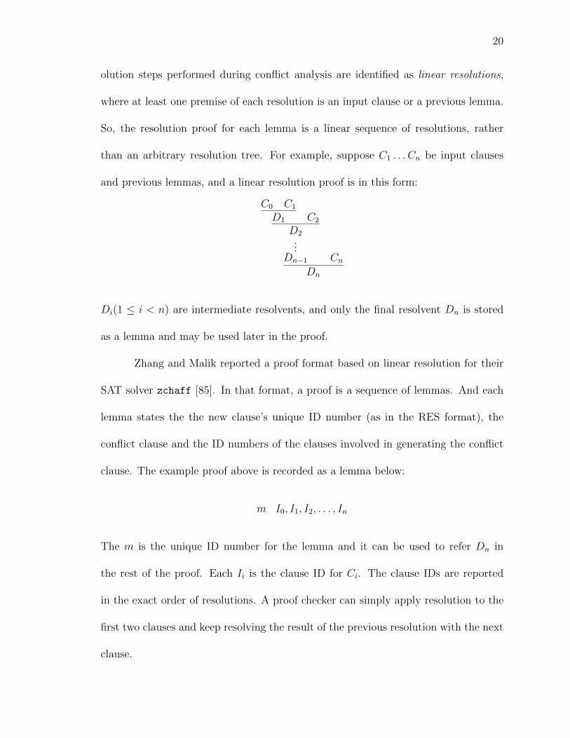
olution steps performed during conflict analysis are identified as linear resolutions,
where at least one premise of each resolution is an input clause or a previous lemma.
So, the resolution proof for each lemma is a linear sequence of resolutions, rather
than an arbitrary resolution tree. For example, suppose C1 . . . Cn be input clauses
and previous lemmas, and a linear resolution proof is in this form:
C0 C1
D1 C2
D2...
Dn−1 Cn
Dn
Di(1 ≤ i < n) are intermediate resolvents, and only the final resolvent Dn is stored
as a lemma and may be used later in the proof.
Zhang and Malik reported a proof format based on linear resolution for their
SAT solver zchaff [85]. In that format, a proof is a sequence of lemmas. And each
lemma states the the new clause’s unique ID number (as in the RES format), the
conflict clause and the ID numbers of the clauses involved in generating the conflict
clause. The example proof above is recorded as a lemma below:
m I0, I1, I2, . . . , In
The m is the unique ID number for the lemma and it can be used to refer Dn in
the rest of the proof. Each Ii is the clause ID for Ci. The clause IDs are reported
in the exact order of resolutions. A proof checker can simply apply resolution to the
first two clauses and keep resolving the result of the previous resolution with the next
clause.
21
PicoSAT is one of the state-of-the-art SAT solvers. The PicoSAT developers
designed their own proof format, called TraceCheck. TraceCheck is very similar to
the zchaff’s proof trace. But, TraceCheck can optionally report Dn along with the
clause IDs, which is useful for debugging. When not reported, Dn is abbreviated with
a wildcard symbol ∗. For example, the same lemma above can be stated as:
m Dn I0, I1, I2, . . . , Inor
m ∗ I0, I1, I2, . . . , In
Unlike zchaff’s trace format, TraceCheck format allows the clause IDs to be reported
in an arbitrary order. That makes it considerably easier to instrument existing SAT
solvers to report proofs. Any TraceCheck checker should be able to calculate the
correct order of resolutions.
These linear resolution-based formats can shrink proofs even further compared
to the RES/RPT formats. Linear resolution is known to be refutation complete [38].
So, it is true that any solver can report a linear resolution proof. Moreover, it is
also easier for most mainstream SAT solvers to report using these formats, especially
TraceCheck [19].
3.1.3 Reverse Unit Propagation
The Reverse Unit Propagation (RUP) proof format has been proposed by Van
Gelder as an efficient propositional proof representation scheme [38]. RUP is an infer-
ence rule that concludes F ` C when (F ∪¬C) is refutable using only unit resolution,
which is similar to standard binary resolution except that one of the two resolved
clauses is required to be a unit clause. Unit resolution is not refutation complete in
general, but it has been shown that conflict clauses generated from standard conflict-
22
analysis algorithms are indeed RUP inferences [38]. If a clause is a RUP inference,
a unit-resolution proof deriving the clause can be calculated from that clause itself.
Potentially, a long resolution proof of a RUP inference can be compressed to the
concluded clause. Also, an efficient RUP inference checker can be implemented using
the two-literal watch lists, a standard unit propagation algorithm used in most SAT
solvers [41]. A complete RUP proof is a sequence of clauses (lemmas) with the last
one being the empty clause. The clauses are checked one clause at a time. Each
clause C is checked with respect to the RUP inference rule, where F is the original
formula and the clauses that have been checked previously. Even though all cor-
rect lemmas are logically true in the input formula, RUP inference is so weak that
intermediate clauses are necessary as stepping stones leading to the empty clause.
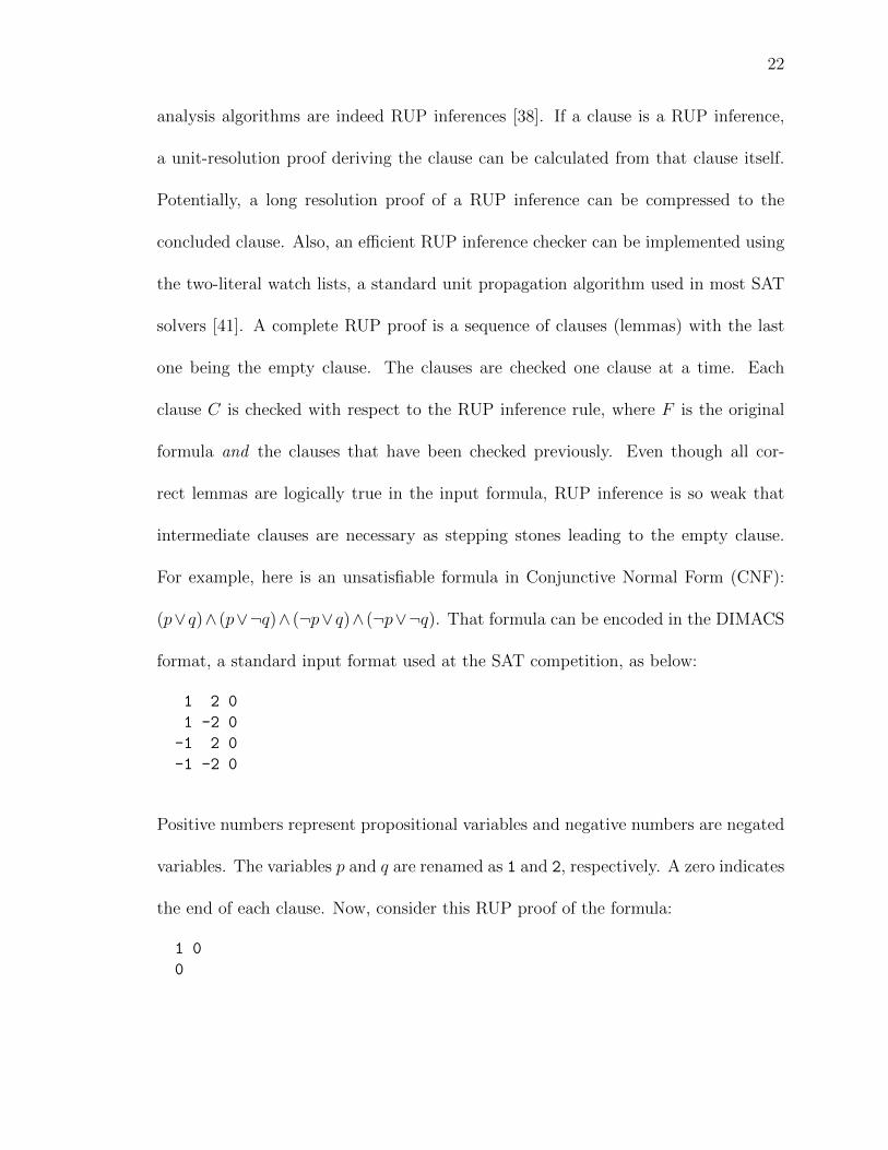
For example, here is an unsatisfiable formula in Conjunctive Normal Form (CNF):
(p∨q)∧ (p∨¬q)∧ (¬p∨q)∧ (¬p∨¬q). That formula can be encoded in the DIMACS
format, a standard input format used at the SAT competition, as below:
1 2 0
1 -2 0
-1 2 0
-1 -2 0
Positive numbers represent propositional variables and negative numbers are negated
variables. The variables p and q are renamed as 1 and 2, respectively. A zero indicates
the end of each clause. Now, consider this RUP proof of the formula:
1 0
0

23
An equivalent TraceCheck proof would be:
5 p 1, 26 ⊥ 3, 4, 5
The RUP proof format has a similar syntax as the DIMACS format. The proof
above has two clauses (RUP inferences). Essentially, it is the same as the TraceCheck
version above, except that all the proof annotations are missing in the RUP proof.
Because the input formula does not have a unit clause, the empty clause cannot be a
RUP inference directly from the input formula. So, at least one intermediate clause is
necessary. The first proof clause is a unit clause 1. Assume the negation of the clause,
which is -1. The assumed clause -1 and the first clause of the formula concludes 2 by
unit resolution, and similarly, -1 and the second clause concludes -2. Finally, 2 and
-2 are contradictory. So, 1 is a RUP inference. Once a clause is verified, it is kept
as a lemma and may be used in the later inferences. Using the clause just verified,
the empty clause can be checked in a similar fashion, resolving 1 with the third and
fourth input clauses.
Almost all mainstream SAT solvers are clause learning SAT solvers with a
form of conflict analysis. Because such learned clauses are RUP inferences, the RUP
format is even easier to instrument in existing SAT solvers than TraceCheck. Thus,
the RUP format is the most popular format used at the SAT competition.
3.1.4 Trustworthiness of the Proof Checker
The official proof checker, checker3 for the SAT competition, is 1,538 lines
of C. It supports RES and RPT formats. An efficient RUP proof checker would be
more complex, because RUP proof checking requires a quite sophisticated algorithm

24
to achieve desired performance. In the SAT competition, RUP proofs are converted
to RES format first. Then, the RES version is checked. This conversion, however,
does not need verification. It’s considered an immediate step of proof construction,
and the final RES proofs are used to certify the unsatisfiability of the formula. The
disadvantage is, due to this conversion process the official RUP checker failed to
check many proofs at the competitions. The PicoSAT developers’ own proof checker,
tracecheck is very efficient, but the size of trusted base is quite huge (2,989 lines of
C++ and the boolforce library), considering the best SAT solver minisat is about
2,500 lines of C++. To construct more trustworthy proof checkers, two methods have
been proposed:
Proof reconstruction in theorem provers. Weber implemented a proof checker
in the Isabelle theorem prover [79, 78, 80]. Any SAT solver can be used as an ex-
ternal oracle, and his checker translates the propositional proofs generated from the
SAT solver to the theorem prover’s own proof objects so that the theorem φ ` ⊥ is
justified by the theorem prover’s kernel. This kind of proof checking is called proof
reconstruction. Proof reconstruction-based checkers can also be used as tactics within
the theorem prover, not just as proof checkers.
Verifying proof checker Darbari et al. implemented an efficient TraceCheck proof
checker and verified its soundness (it only accepts correct proofs) in the Coq theorem
prover [29]. This technique does not translate proofs, instead it checks proofs directly.
They can also extract a certified OCaml code, which is executable independently of
25
the theorem prover.
3.2 SMT Proof Checking
Considering the size and complexity of modern SMT solvers, it seems much
more difficult to verify their code. Instead, it may be more cost-effective to verify
their proofs. CVC3 [55, 36], Fx7 [57], Z3 [31], and veriT [22] are example SMT solvers
that have the ability to produce refutation proofs. Unlike SAT, there is no de facto
standard format for SMT proofs. Those solvers defined their own proof formats, and
there are no separate authorities or official formats, yet.
CVC3. CVC3’s proofs are in the format of the HOL Light theorem prover (a LCF-
style theorem prover), while others use their own custom proof formats. CVC3’s
proofs are translated to HOL Light’s proofs and construct theorems in the theorem
prover (proof reconstruction).
Fx7. Moskal’s Fx7 uses a custom rewriting-based meta-language to enable concise
and understandable expression of proof rules, to increase trust. He also implemented
a meta-language checker, Trew, which is shown to be very efficient for the AUFLIA
(Linear Integer Arithmetic with Uninterpreted Functions and Arrays) logic bench-
marks in the SMT-LIB database. Trew’s code is 1,500 lines of C, which is small, but
still less trustworthy than small-core theorem provers written in functional program-
ming languages.
26
Z3. Z3 uses a particular natural deduction proof system. At first, a custom proof
checker was used mostly for debugging of Z3 itself. Recently, Bohme et al. imple-
mented a proof reconstruction-based checker in Isabelle [21].
veriT. The proof format of veriT has its own natural deduction rules with a linear
layout, in which each deduction step makes a new line with a line number. Armand et
al. implemented a verified proof checker for veriT’s proofs in Coq [10]. They showed
that proof checking is more efficient than compared to Bohme et al’s method because
they do not reconstruct Coq proofs from veriT’s proofs. Previously, Fontaine et al.
also showed a proof reconstruction method in Isabelle with the previous version of
veriT, called haRVey [34]. They report that proof reconstruction (proof checking in
Isabelle) takes exceedingly longer time compared to proof-searching time taken by
the haRVey prover.
3.3 Statically Verified SAT Solvers
Verifying the SAT solver’s code means proving some of these theorems about
it.
1. If solve(φ) = SAT , then ∃M.M φ.
2. If solve(φ) = UNSAT , then ∀M.M 2 φ.
3. solve is a total function (always terminates).
The properties 1 and 2 are the soundness (answers are correct) of the algo-
rithm. The property 3 is the completeness (questions are eventually answered) of the
27
algorithm.
3.3.1 Verified SAT Solvers
Noteworthy efforts have been made to apply formal verification techniques to
SAT solver algorithms, using interactive theorem provers. Following researchers have
proved their solvers are sound and complete.
1. Lescuyer implemented and verified the classical DPLL algorithm in Coq [51].
He proved that the algorithm is sound and complete according to the standard
semantics of propositional logic. His work is an effort to bring the DPLL proce-
dure directly into Coq as a fully automated propositional reasoning tactic. His
implementation can also be extracted into the OCaml programming language
and compiled to machine code. However, the classical DPLL algorithm is not
as efficient as the modern DPLL implementations, setting aside the overhead of
the OCaml runtime environment due to garbage collection.
2. Maric implemented a modern style DPLL algorithm in Isabelle, including con-
flict analysis, clause learning and backjumping features [53]. He also imple-
mented one of the low-level features: the two-literal watch lists. Maric verified
that the algorithm is sound and complete. The specification of correct SAT
solver is based on the abstract DPLL state transition rules [61]. Abstract DPLL
is a formalization of the SAT algorithm in terms of a state transition system,
instead of imperative pseudocode as in the classical DPLL. It is a more gen-
eralized framework that accommodates new features and deduction methods

28
of modern solvers. Even though he implemented some low-level details, this
implementation is not executable outside the theorem prover and it serves as a
model of the actual C++ implementation.
3. Shankar et al. also proved a modern DPLL algorithm in the PVS theorem
prover [69]. This implementation has modern features like clause learning and
backjumping, and it is also verified to be sound and complete according to the
abstract DPLL state transition rules. Compared to Maric’s implementation, it
lacks a low-level detail like the two-literal watch lists.
These SAT solvers are verified in various theorem provers. Lescuyer’s imple-
mentation can also be used as a trusted tactic for the Coq theorem prover because
this implementation is executable and certified. The other implementations did not
implement decision heuristics, because such heuristics do not affect the correctness of
the solvers. Their decision heuristics are left as abstract choice functions. Although
any simple heuristic can replace the abstract functions, a more realistic heuristic will
call for a feedback mechanism from the other parts of the solver, and thus significant
refactoring of the solver may be necessary.
3.3.2 Limitations
The biggest limitation of the verified SAT solvers is the performance. None of
these SAT solvers are intended to match the performance of unverified SAT solvers.
Those verified SAT solvers above either use inefficient data structures or omit low-
level details to simplify verification. For example, Peano numbers or abstract data

29
type are used to represent propositional variables of the input formula, where as
mainstream SAT solvers use machine words for efficiency. An abstract data type can
be replaced with machine words during compilation of such a verified SAT solver;
however the details related to bit/arithmetic operations and overflow situations are
hidden and abstracted away from the solver implementation. Maric’s implementation
uses a list (instead of an array) to represent the entire clause database and perform
sequential access to individual clauses. Shankar’s implementation is more optimized
using an array data structure for the clause database and perform random access
to clauses. Mainstream SAT solvers use low-level data structures such as machine
words, bit operations, mutable arrays and pointers. Also, they are highly optimized
using various engineering techniques, such as splitting, duplicating, and reorganizing
data in memory for faster access. Most of these engineering techniques do not appear
in the verified solvers, and they can not be easily implemented in the programming
language of theorem provers. For example:
• Because each clause is referenced by several pointers in the two-literal watch
lists and other data structures, the whole data structure becomes a graph
(rather than a tree), which makes it difficult to implement in such program-
ming languages In the Maric and Shankar’s implementations, clauses in the
clause database are accessed indirectly through their position numbers in the
list (or array) of all clauses. On the other hand, in mainstream SAT solvers,
clauses are not numbered; instead, they are directly referenced. Thus, there is
no single list or array referencing all the clauses. Directly referencing clauses is

30
an important low-level optimization that significantly affects the performance.
• Mutable arrays are critical to the performance of SAT solvers. The two-literal
watch lists are a collection of arrays that change dynamically. Also, solvers use
a variety of lookup tables for bookkeeping purposes. Therefore, the support for
efficient mutable arrays is important for implementing high-performance SAT
solvers.

31
CHAPTER 4
SAT/SMT PROOF CHECKING USING A LOGICAL FRAMEWORK
There are many different SMT logics depending on the theories built into the
logics. The SMT-LIB initiative provides a library of formulas divided into several
different logics. Even though SMT-LIB defines a set of standard theories and logics,
solvers may support for novel logics by adding their own theories. Also, different SMT
solvers may use different sets of inference rules depending on the solver’s algorithms.
So, a flexible and extensible proof system is highly desirable for a standard SMT
proof checker. As shown in Section 3.2, Both CVC3 and Fx7 use meta-languages as
the bases of their proof format. CVC3 generates proofs in the HOL Light’s proof
language. Because HOL Light can be extended with new theories, the logic of HOL
Light can be considered a meta-language to encode inference rules (a logic) and
proofs. Fx7 uses its own meta-language, called Trew, which is specifically designed
for encoding logics and efficient proof checking. Trew is based on a term-rewriting
calculus. In Trew, inference rules (at the logic level) are encoded as rewrite rules (at
the meta-language level). The advantage of using a meta-language is that the proof
checker can be easily extended. Usually inference rules are defined declaratively and
modularly, thus it is easy to understand and verify the existing rules, and add new
rules. If we compare that to the program code for a proof checker, the code may
be obscure to understand and adding new rules may change the meaning of the old
code for the existing rules, which can break the correctness of the old code. For
32
the other proof formats discussed in Section 3.2, theorem provers are still used to
validate proofs. Bohme et al. essentially implemented a proof translator from an
ad-hoc proof language to the proof language of the Isabelle/HOL theorem prover.
Besides the translation part, everything is the same as CVC3 proofs in HOL Light.
Armand et al. verified their proof checker is correct in the Coq theorem prover. This
proof checker does not translate proofs, instead they proved that the proof checker’s
computation is sound w.r.t the encoding of the logic. As we can see, all of the SMT
proof systems above rely on meta-languages one way or another to encode the subject
logic and ensure the correctness of the proof checkers. In this chapter, we describe a
novel SMT proof system based on another meta-language, called Edinburgh Logical
Framework.
4.1 The LFSC Language
In this chapter we propose and describe a meta-logic, called LFSC, for “Log-
ical Framework with Side Conditions”, which we have developed explicitly with the
goal of supporting the description of several proof systems for SMT, and enabling the
implementation of very fast proof checkers. In LFSC, solver implementors can de-
scribe their proof rules using a compact declarative notation which also allows the use
of computational side conditions. These conditions, expressed in a small functional
programming language, enable some parts of a proof to be established by computa-
tion. The flexibility of LFSC facilitates the design of proof systems that reflect closely
the sort of high-performance inferences made by SMT solvers. The side conditions
feature offers a continuum of possible LFSC encodings of proof systems, from com-
33
pletely declarative at one extreme, using rules with no side conditions, to completely
computational at the other, using a single rule with a huge side condition. We argue
that supporting this continuum is a major strength of LFSC. Solver implementors
have the freedom to choose the amount of computational inference when devising
proof systems for their solver. This freedom cannot be abused since any decision is
explicitly recorded in the LFSC formalization and becomes part of the proof system’s
trusted computing base. Moreover, the ability to create with a relatively small effort
different LFSC proof systems for the same solver provides an additional level of trust
even for proof systems with a substantial computational component—since at least
during the developing phase one could also produce proofs in a more declarative, if
less efficient, proof system.
We have put considerable effort in developing a full blown, highly efficient proof
checker for LFSC proofs. Instead of developing a dedicated LFSC checker, one could
imagine embedding LFSC in declarative languages such as Maude or Haskell. While
the advantages of prototyping symbolic tools in these languages are well known, in our
experience their performance lags too far behind carefully engineered imperative code
for high-performance proof checking. This is especially the case for the sort of proofs
generated by SMT solvers which can easily reach sizes measured in megabytes or
even gigabytes. Based on previous experimental results by others, a similar argument
could be made against the use of interactive theorem provers (such as Isabelle [63] or
Coq [18]), which have a very small trusted core, for SMT-proof checking. By allowing
the use of computational side conditions and relying on a dedicated proof checker,

34
our solution seeks to strike a pragmatic compromise between trustworthiness and
efficiency.
4.1.1 Notational Conventions
LFSC is a direct extension of Edinburgh Logical Framework (LF, for short) [46],
a type-theoretic logical framework based on the λΠ calculus, in turn an extension of
the simply typed λ-calculus. A logical framework in the general sense is a language (or
a system) that allows for encoding axioms and inference rules, and checking proofs.
LF influenced the early theorem prover, Automath and others like Coq and Twelf. LF
has been used successfully for representing proofs in applications like proof-carrying
code [59].
The λΠ calculus has three levels of entities: values ; types, understood as
collections of values; and kinds, families of types. Its main feature is the support
for dependent types which are types parametrized by values.1 Informally speaking, if
τ2[x] is a dependent type with value parameter x, and τ1 is a non-dependent type,
the expression Πx:τ1.τ2[x] denotes in the calculus the type of functions that return a
value of type τ2[v] for each value v of type τ1 for x. When τ2 is itself a non-dependent
type, the type Πx:τ1.τ2 is just the arrow type τ1 → τ2 of simply typed λ-calculus.
The current concrete syntax of LFSC is based on Lisp-style S-expressions,
with all operators in infix format. For improved readability, we will often write LFSC
expressions in abstract syntax instead. We will write concrete syntax expressions in
1 A simple example of dependent types is the type of bit vectors of (positive integer)size n.
35
typewriter font. In abstract syntax expressions, we will write variables and meta-
variables in italics font, and constants in sans serif font. Predefined keywords in the
LFSC language will be in bold sans serif font.
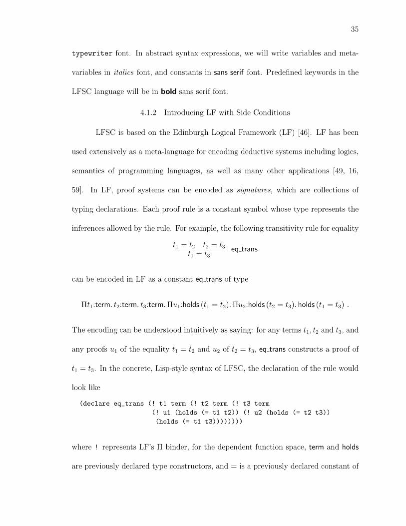
4.1.2 Introducing LF with Side Conditions
LFSC is based on the Edinburgh Logical Framework (LF) [46]. LF has been
used extensively as a meta-language for encoding deductive systems including logics,
semantics of programming languages, as well as many other applications [49, 16,
59]. In LF, proof systems can be encoded as signatures, which are collections of
typing declarations. Each proof rule is a constant symbol whose type represents the
inferences allowed by the rule. For example, the following transitivity rule for equality
t1 = t2 t2 = t3t1 = t3
eq trans
can be encoded in LF as a constant eq trans of type
Πt1:term. t2:term. t3:term.Πu1:holds (t1 = t2).Πu2:holds (t2 = t3). holds (t1 = t3) .
The encoding can be understood intuitively as saying: for any terms t1, t2 and t3, and
any proofs u1 of the equality t1 = t2 and u2 of t2 = t3, eq trans constructs a proof of
t1 = t3. In the concrete, Lisp-style syntax of LFSC, the declaration of the rule would
look like
(declare eq_trans (! t1 term (! t2 term (! t3 term
(! u1 (holds (= t1 t2)) (! u2 (holds (= t2 t3))
(holds (= t1 t3))))))))
where ! represents LF’s Π binder, for the dependent function space, term and holds
are previously declared type constructors, and = is a previously declared constant of

36
type Πt1:term. t2:term. term (i.e., term→ term→ term).
Now, pure LF is not well suited for encoding large proofs from SMT solvers,
due to the computational nature of many SMT inferences. For example, consider
trying to prove the following simple statement in a logic of arithmetic:
(t1 + (t2 + (. . .+ tn) . . .))− ((ti1 + (ti2 + (. . .+ tin) . . .) = 0 (4.1)
where ti1 . . . tin is a permutation of the terms t1, . . . , tn. A purely declarative proof
would need Ω(n log n) applications of an associativity and a commutativity rule for
+, to bring opposite terms together before they can be pairwise reduced to 0.
Producing, and checking, purely declarative proofs in SMT, where input for-
mulas alone are often measured in megabytes, is unfeasible in many cases. To address
this problem, LFSC extends LF by supporting the definition of rules with side con-
ditions, computational checks written in a small but expressive first-order functional
language. The language has built-in types for arbitrary precision integers and ratio-
nals, inductive datatypes, ML-style pattern matching, recursion, and a very restricted
set of imperative features. When checking the application of an inference rule with a
side condition, an LFSC checker computes actual parameters for the side condition
and executes its code. If the side condition fails, because it is not satisfied or because
of an exception caused by a pattern-matching failure, the LFSC checker rejects the
rule application. In LFSC, a proof of statement (4.1) could be given by a single
application of a rule of the form:
(declare eq_zero (! t term (^ (normalize t) 0) (holds (= t 0))))
where normalize is the name of a separately defined function in the side condition

37
(Kinds) κ ::= type | kind | Πx:τ. κ
(Types) τ ::= k | τ t | Πx:τ1[s t]. τ2(Terms) t ::= x | c | t:τ | λx[:τ ]. t | t1 t2(Patterns) p ::= c | c x1 · · ·xn+1
(Programs) s ::= x | c | c s1 · · · sn+1 | match s (p1 s1) · · · (pn+1 sn+1) |let x s1 s2 | fail τ | −s | s1 + s2 | s1 × s2 | ifneg s1 s2 s3 |markvar s | ifmarked s1 s2 s3
Figure 4.1. Main syntactical categories of LFSC. Letter c denotes term constants(including integer/rational ones), x denotes term variables, k denotes type constants.The square brackets are grammar meta-symbols enclosing optional subexpressions.
language that takes an arithmetic term and returns a normal form for it. The expres-
sion (^ (normalize t) 0) defines the side condition of the eq zero rule, with the
condition succeeding if and only if the expression (normalize t) evaluates to 0.
4.1.3 Abstract Syntax and Informal Semantics
In this section, we informally describe the LFSC language in abstract syntax
and its informal semantics. The formal typing rules and semantics of LFSC is dis-
cussed in Appendices A.1 and A.2. Well-typed value, type, kind and side-condition
expressions are drawn from the syntactical categories defined in Figure 4.1 in BNF
format. The syntax for kinds, types, and terms is the same as the orignal LF, except
for the optional side condition expression in the Π-abstraction. And the syntax for
patterns and programs is added to express side condition programs. Programs can be
defined and given names so that they can be called from side condition expressions.
Also, note that programs can be called recursively within the program itself without

38
restriction, which permits general recursion. Currently, we do not enforce termination
of side condition programs, nor do we attempt to provide facilities to reason formally
about the behavior of such programs.
Program expressions s are used in side condition code. There, we also make use
of the syntactic sugar (do s1 · · · sn s) for the expression (let x1 s1 · · · let xn sn s) where
x1 through xn are fresh variables. Side condition programs in LFSC are monomorphic,
simply typed, first-order, recursive functions with pattern matching, inductive data
types and two built-in basic types: arbitrary precision integers and rationals. In
practice, our implementation is a little more permissive, allowing side-condition code
to pattern-match also over dependently typed data. For simplicity, we restrict our
attention here to the formalization for simple types only.
The operational semantics of the main constructs in the side condition lan-
guage could be described informally as follows. Expressions of the form s t is a
restrictive form of equality predicates, meaning that the expression s evaluates to
the term t. Expressions of the form (c s1 · · · sn+1) are applications of either term
constants or program constants (i.e., declared functions) to arguments. In the former
case, the application constructs a new value; in the latter, it invokes a program. The
expressions (match s (p1 s1) · · · (pn+1 sn+1)) and (let x s1 s2) behave exactly as their
corresponding matching and let-binding constructs in ML-like languages. The expres-
sion (fail τ) always raises that exception, for any type τ . The expression (markvar s)
evaluates to the value of s if this value is a variable. In that case, the expression has

39
also the side effect of toggling a Boolean mark on that variable. 2 The expression
(ifmarked s1 s2 s3) evaluates to the value of s2 or of s3 depending on whether s1
evaluates to a marked or an unmarked variable. Both markvar and ifmarked raise
a failure exception if their arguments do not evaluate to a variable. We support
marking just variables instead of arbitrary terms, because it is convenient to map all
occurrences of the same (as determined by scoping) variable to the same in-memory
representation. The same is not true for arbitrary terms, particularly in the presence
of a non-trivial definitional equality: an indexing structure would then be needed,
imposing additional implementation complexity and runtime performance penalty.
Type checking also fails when evaluating the fail construct (fail τ), or when pattern
matching fails.
LFSC has two built-in numeric types: mpz and mpr. The mpz type is for
arbitrary precision integer type (the name comes from the underlying GNU Multiple
Precision Arithmetic Library, gmp); the mpr type is similarly for rationals. Also,
LFSC provides built-in arithmetic functions overloaded for those types: −(unary),
+, ×, and ifneg. The arguments to these functions must be numeric expressions of
the same type. The first three functions operates on numeric constants as expected;
(ifneg x y z) evaluates to y or z depending on whether the mpz number x is negative
or not.
Our implementation of LFSC supports the use of the wildcard symbol in
2 For simplicity, we limit the description here to a single mark per variable. In reality,there are 32 such marks, each with its own markvar command.

40
place of an actual argument of an application when the value of this argument is
determined by the types of later arguments. This feature, which is analogous to
implicit arguments in theorem provers such as Coq and programming languages such
as Scala, is crucial to avoid bloating proofs with redundant information. In a similar
vein, the syntax allows a form of lambda abstraction that does not annotate the bound
variable with its type when that type can be computed efficiently from context.
4.2 Encoding Propositional Reasoning
In this section and the next, we illustrate the power and flexibility of LFSC for
SMT proof checking by discussing a number of proof systems relevant to SMT, and
their possible encodings in LFSC. Our goal is not to be exhaustive, but to provide
representative examples of how LFSC allows one to encode a variety of logics and
proof rules while paying attention to proof checking performance issues. Section 4.4
focuses on the latter by reporting on our initial experimental results.
Roughly speaking, proofs generated by SMT solvers, especially those based on
the DPLL(T ) architecture [62], are two-tiered refutation proofs, with a propositional
skeleton filled with several theory-specific subproofs [40]. The conclusion, a trivially
unsatisfiable formula, is reached by means of propositional inferences applied to a set
of input formulas and a set of theory lemmas. These are disjunctions of theory literals
proved from no assumptions mostly with proof rules specific to the theory or theories
in question—the theory of real arithmetic, of arrays, etc.
Large portions of the proof’s propositional part consist typically of applications
of some variant of the resolution rule. These subproofs are generated similarly to what

41
is done by proof-producing SAT solvers, where resolution is used for conflict analysis
and lemma generation [84, 40]. A proof format proposed in 2005 by Van Gelder for
SAT solvers is based directly on resolution [75]. Input formulas in SMT differ from
those given to SAT solvers both for being not necessarily in Conjunctive Normal
Form and for having non-propositional atoms. As a consequence, the rest of the
propositional part of SMT proofs involve CNF conversion rules as well as abstraction
rules that uniformly replace theory atoms in input formulas and theory lemmas with
Boolean variables. While SMT solvers usually work just with quantifier-free formulas,
some of them can reason about quantifiers as well, by generating and using selected
ground instances of quantified formulas. In these cases, output proofs also contain
applications of rules for quantifier instantiation.
In the following, we demonstrate different ways of representing propositional
clauses and SMT formulas and lemmas in LFSC, and of encoding proof systems for
them with various degrees of support for efficient proof checking. For simplicity and
space constraints, we consider only a couple of individual theories, and restrict our
attention to quantifier-free formulas. We note that encoding proofs involving com-
binations of theories is more laborious but not qualitatively more difficult; encoding
SMT proofs for quantified formulas is straightforward thanks to LFSC’s support for
higher-order abstract syntax which allows one to represent and manipulate quantifiers
as higher-order functions, in a completely standard way.3
3 For instance ∀x:τ. φ can be represented as (forall λx:τ. φ) where forall is a constant oftype (τ → formula) → formula. Then, quantifier instantiation reduces to (lambda-term)application.

42
(declare var type)
(declare lit type)
(declare pos (! x var lit))
(declare neg (! x var lit))
(declare clause type)
(declare cln clause)
(declare clc (! l lit (! c clause clause)))
Figure 4.2. Definition of propositional clauses in LFSC concrete syntax
4.2.1 Encoding Propositional Resolution
The first step in encoding any proof system in LFSC (or LF for that matter)
is to encode its formulas. In the case of propositional resolution, this means encoding
propositional clauses. Figure 4.2 presents a possible encoding, with type and type
constructor declarations in LFSC’s concrete syntax. We first declare an LFSC type
var for propositional variables and then a type lit for propositional literals. Type lit
has two constructors, pos and neg, both of type Πx:var. lit4 which turn a variable into
a literal of positive, respectively negative, polarity. We use these to represent positive
and negative occurrences of a variable in a clause. The type clause, for propositional
clauses, is endowed with two constructors that allow the encoding of clauses as lists of
literals. The constant cln represents the empty clause (). The function clc intuitively
takes a literal l and a clause c, and returns a new clause consisting of l followed by
the literals of c. For an example, a clause like P ∨ ¬Q can be encoded as the term
(clc (pos P ) (clc (neg Q) cln)).
4 Recall that the ! symbol in the concrete syntax stands for Π-abstraction.
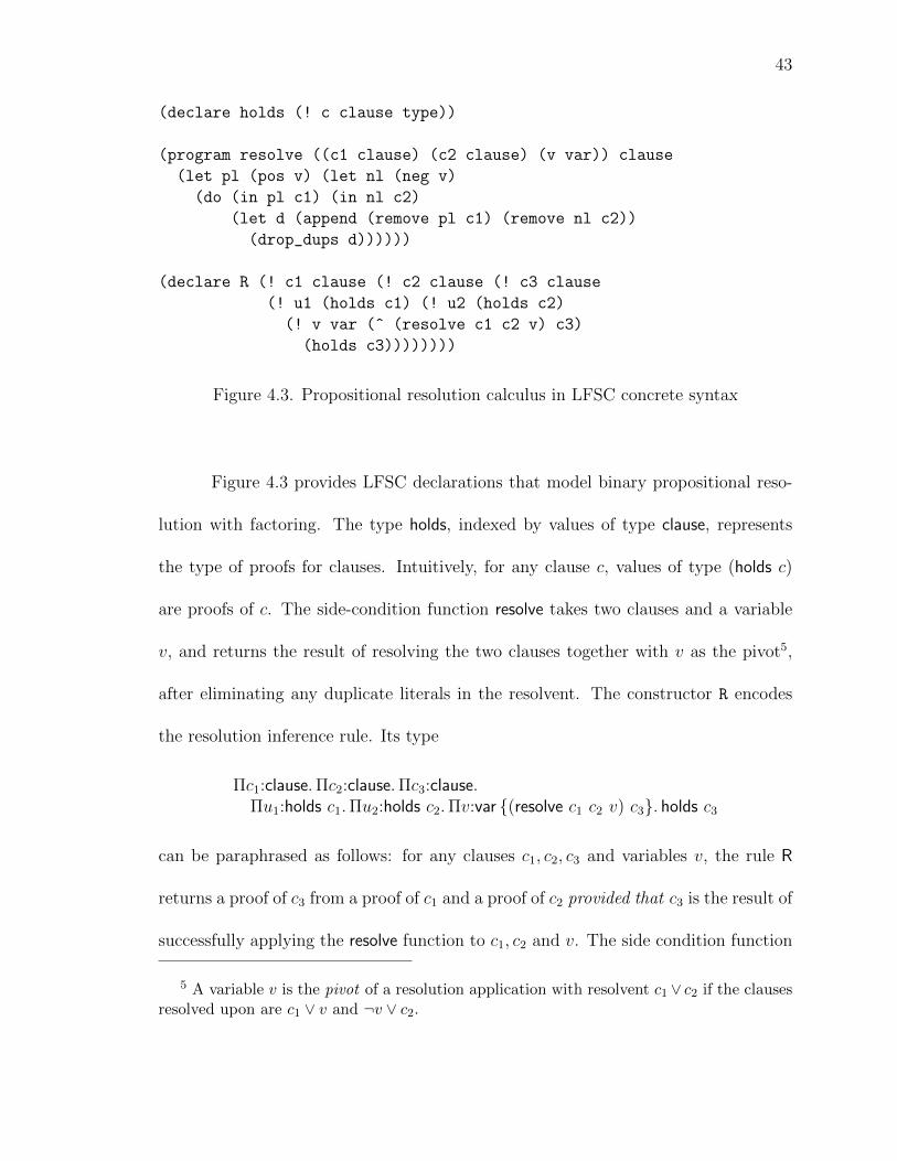
43
(declare holds (! c clause type))
(program resolve ((c1 clause) (c2 clause) (v var)) clause
(let pl (pos v) (let nl (neg v)
(do (in pl c1) (in nl c2)
(let d (append (remove pl c1) (remove nl c2))
(drop_dups d))))))
(declare R (! c1 clause (! c2 clause (! c3 clause
(! u1 (holds c1) (! u2 (holds c2)
(! v var (^ (resolve c1 c2 v) c3)
(holds c3))))))))
Figure 4.3. Propositional resolution calculus in LFSC concrete syntax
Figure 4.3 provides LFSC declarations that model binary propositional reso-
lution with factoring. The type holds, indexed by values of type clause, represents
the type of proofs for clauses. Intuitively, for any clause c, values of type (holds c)
are proofs of c. The side-condition function resolve takes two clauses and a variable
v, and returns the result of resolving the two clauses together with v as the pivot5,
after eliminating any duplicate literals in the resolvent. The constructor R encodes
the resolution inference rule. Its type
Πc1:clause.Πc2:clause.Πc3:clause.Πu1:holds c1.Πu2:holds c2.Πv:var (resolve c1 c2 v) c3. holds c3
can be paraphrased as follows: for any clauses c1, c2, c3 and variables v, the rule R
returns a proof of c3 from a proof of c1 and a proof of c2 provided that c3 is the result of
successfully applying the resolve function to c1, c2 and v. The side condition function
5 A variable v is the pivot of a resolution application with resolvent c1 ∨ c2 if the clausesresolved upon are c1 ∨ v and ¬v ∨ c2.

44
resolve is defined as follows (using a number of auxiliary functions whose definition
can be found in the appendix). To resolve clauses c1 and c2 with pivot v, v must occur
in a positive literal of c1 and a negative literal of c2 (checked with the in function).
If that case, the resolvent clause is computed by removing (with remove) all positive
occurrences of v from c1 and all negative ones from c2, concatenating the resulting
clauses (with append), and finally dropping any duplicates from the concatenation
(with drop dups); otherwise, resolve, and consequently the side condition of R, fails.
In proof terms containing applications of the R rule, the values of its input
variables c1, c2 and c3 can be determined from later input values, namely the concrete
types of u1, u2 and v, respectively. Hence, in those applications c1, . . . , c3 can be
replaced by the wildcard , as mentioned in Section 4.1 and shown in Figure 4.4.
The single rule above is enough to encode proofs in the propositional resolution
calculus. This does not appear to be possible in LF. Without side conditions one also
needs auxiliary rules, for instance, to move a pivot to the head of the list representing
the clause and to perform factoring on the resolvent. The upshot of this is a more
complex proof system and bigger proofs. Other approaches to checking resolution
proofs avoid the need for those auxiliary rules by hard coding the clause type in
the proof checker and implementing it as a set of literals. An example is work by
Weber and Amjad on reconstructing proofs produced by an external SAT solver in
Isabelle/HOL [81]. They use several novel encoding techniques to take advantage
of the fact that the native sequents of the Isabelle/HOL theorem prover are of the
form Γ ` φ, where Γ is interpreted as a set of literals. They note the importance of

45
V1 ∨ V2 ¬V1 ∨ V2V2
¬V2 ∨ V3 ¬V3 ∨ ¬V2¬V2
λv1:var. λv2:var. λv2:var.
λp1:holds (v1 ∨ v2). λp2:holds (¬v1 ∨ v2).λp3:holds (¬v2 ∨ v3). λp4:holds (¬v3 ∨ ¬v2).
(R (R p1 p2 v1) (R p3 p4 v3) v2) : holds )
(check
(% v1 var (% v2 var (% v3 var
(% p1 (holds (clc (pos v1) (clc (pos v2) cln)))
(% p2 (holds (clc (neg v1) (clc (pos v2) cln)))
(% p3 (holds (clc (neg v2) (clc (pos v3) cln)))
(% p4 (holds (clc (neg v3) (clc (neg v2) cln)))
(: (holds cln) (R _ _ _ (R _ _ _ p1 p2 v1)
(R _ _ _ p3 p4 v3) v2))))))))))
Figure 4.4. An example refutation and its LFSC encoding, respectively in abstractand in concrete syntax (as argument of the check command). In the concrete syntax,(% x τ t) stands for λx:τ. t; for convenience, the ascription operator : takes first atype and then a term.
these techniques for achieving acceptable performance over their earlier work, where
rules for reordering literals in a clause, for example, were required. Their focus is on
importing external proofs into Isabelle/HOL, not trustworthy efficient proof-checking
in its own right. But we point out that it would be wrong to conclude that their
approach is intrinsically more declarative than the LFSC approach: in their case, the
computational side-conditions needed to maintain the context Γ as a set have simply
been made implicit, as part of the core inference system of the theorem prover. In
contrast, the LFSC approach makes such side conditions explicit, and user-definable.
Example 1. For a simple example of a resolution proof, consider a propositional

46
clause set containing the clauses c1 := ¬V1 ∨V2, c2 := ¬V2 ∨V3, c3 := ¬V3 ∨¬V2, and
c4 := V1 ∨ V2. A resolution derivation of the empty clause from these clauses is given
in Figure 4.4. The proof can be represented in LFSC as the lambda term below the
proof tree. Ascription is used to assign type (holds ) to the main subterm (R . . . v2)
under the assumption that all four input clauses hold. This assumption is encoded
by using the input (i.e., lambda) variables p1, . . . , p4 of type (holds c1), . . . , (holds c4),
respectively. Checking the correctness of the original proof in the resolution calculus
then amounts to checking that the lambda term is well-typed in LFSC when its holes
are filled in as prescribed by the definition of R. In the concrete syntax, this is achieved
by passing the proof term to the check command.
The use of lambda abstraction in the example above comes from standard LF
encoding methodology. In particular, note how object-language variables (the Vi’s)
are represented by LFSC meta-variables (the λ-variables v1, . . . , v4). This way, safe
renaming and safe substitution of bound variables at the object level are inherited for
free from the meta-level. In LFSC, an additional motivation for using meta-variables
for object language variables is that we can efficiently test the former for equality in
side conditions using variable marking. In the resolution proof system described here,
this is necessary in the side condition of the R rule—for instance, to check that the
pivot occurs in the clauses being resolved upon (see Appendix A.3).
4.2.2 Deferred Resolution
The single rule resolution calculus presented above can be further improved in
terms of proof checking performance by delaying the side condition tests, as done in

47
(declare clr (! l lit (! c clause clause)))
(declare con (! c1 clause (! c2 clause clause)))
(declare DR (! c1 clause (! c2 clause
(! u1 (holds c1) (! u2 (holds c2) (!v var
(holds (con (clr (pos v) c1) (clr (neg v) c2)))))))))
(declare S (! c1 clause (! c2 clause
(! u (holds c1) (^ (simplify c1) c2)
(holds c2)))))
Figure 4.5. New constructors for the clause type and rules for deferred resolution
function simplify (x : clause) : clause =match x with
cln → clncon c1 c2 → append (simplify c1) (simplify c2)clc l c →
if l is marked for deletion then (simplify c)else mark l for deletion; d = clc l (simplify c); unmark l; d
clr l c →if l is marked for deletion then d = simplify celse mark l for deletion; d = simplify c; unmark l;if l was deleted from c then d else fail
Figure 4.6. Pseudo-code for side condition function used by the S rule
constrained resolution approaches [67]. One can modify the clause data structure so
that it includes constraints representing those conditions. Side condition constraints
are accumulated in resolvent clauses and then checked periodically, possibly just at
the very end, once the final clause has been deduced. The effect of this approach
is that (i) checking resolution applications becomes a constant time operation, and
(ii) side condition checks can be deferred, accumulated, and then performed more

48
efficiently in a single sweep using a new rule that converts a constrained clause to a
regular one after discharging its attached constraint.
There are many ways to implement this general idea. We present one in Fig-
ure 4.5, based on extending the clause type of Figure 4.2 with two more constructors:
clr and con. The term (clr l c) denotes the clause consisting of all the literals of
c except l, assuming that l indeed occurs in c. The expression (con c1 c2) denotes
the clause consisting of all the literals that are in c1 or in c2. Given two clauses c1
and c2 and a pivot variable v, the new resolution rule DR, with no side conditions,
produces the resolvent (con (clr (pos v) c1) (clr (neg v) c2)) which carries within itself
the resolution constraint that (pos v) must occur in c1 and (neg v) in c2. Applications
of the resolution rule can alternate with applications of the rule S, which converts a
resolvent clause into a regular clause (constructed with just cln and clc) while also
checking that the resolvent’s resolution constraints are satisfied. A sensible strategy
is to apply S both to the final resolvent and to any intermediate resolvent that is used
more than once in the overall proof—to avoid unnecessary duplication of constraints.
The side condition function for S is provided in pseudo-code (for improved
readability) in Figure 4.6. The pseudo-code should be self-explanatory. The aux-
iliary function append, defined only on regular clauses, works like a standard list
append function. Since the cost of append is linear in the first argument, simplify
executes more efficiently with linear resolution proofs, where at most one of the two
premises of each resolution step is a previously proved (and simplified) lemma. Such
proofs are naturally generated by SMT solvers with a propositional engine based

49
on conflict analysis and lemma learning—which means essentially all SMT solvers
available today. In some cases, clauses returned by simplify may contain duplicate lit-
erals. However, such literals will be removed by subsequent calls to simplify, thereby
preventing any significant accumulation in the clauses we produce.
Our experiments show that deferred resolution leads to significant performance
improvements at proof checking time: checking deferred resolution proofs is on aver-
age 5 times faster than checking proofs using the resolution rule R [64]. The increased
speed does come here at the cost of increased size and complexity of the side condi-
tion code, and so of the trusted base. The main point is again that LFSC gives users
the choice of how big they want the trusted base to be, while also documenting that
choice explicitly in the side condition code.
4.3 Encoding Quantifier-Free Integer Difference Logic
This section explains our encoding of a sample SMT logic, called Quantifier-
Free Integer Difference Logic (QF IDL, for short). Although QF IDL is one of the
simplest SMT logics, our encoding provides the core infrastructure for all other SMT
logics.
4.3.1 CNF Conversion
Most SMT solvers accept as input quantifier-free formulas (from now on simply
formulas) but do the bulk of their reasoning on a set of clauses derived from the input
via a conversion to CNF or, equivalently, clause form. For proof checking purposes, it
is then necessary to define proof rules that account for this conversion. Defining a good
set of such proof rules is challenging because of the variety of CNF transformations

50
used in practice. Additional difficulties, at least when using logical frameworks, come
from more mundane but nevertheless important problems such as how to encode
with proof rules, which have a fixed number of premises, transformations that treat
operators like logical conjunction and disjunction as multiarity symbols, with an
arbitrary number of arguments.
To show how these difficulties can be addressed in LFSC we discuss now a
hybrid data structure we call partial clauses that mixes formulas and clauses and
supports the encoding of many CNF conversion methods as small step transformations
on partial clauses. Partial clauses represent intermediate states between an initial
formula to be converted to clause form and its final clause form. We then present
a general set of rewrite rules on partial clauses that can be easily encoded as LFSC
proof rules. Abstractly, a partial clause is simply a pair
(φ1, . . . , φm; l1 ∨ · · · ∨ ln)
consisting of a (possibly empty) sequence of formulas and a clause. Semantically, it
is just the disjunction φ1 ∨ · · · ∨ φm ∨ l1 ∨ · · · ∨ ln of all the formulas in the sequence
with the clause. A set φ1, . . . , φk of input formulas, understood conjunctively, can
be represented as the sequence of partial clauses (φ1; ), . . . , (φk; ). A set of rewrite
rules can be used to turn this sequence into an equisatisfiable sequence of partial
clauses of the form ( ; c1), . . . , ( ; cn), which is in turn equisatisfiable with c1∧· · ·∧cn.
Figure 4.7 describes some of the rewrite rules for partial clauses. We defined 31 CNF
conversion rules to transform partial clauses. Most rules eliminate logical connectives
and let-bindings in a similar way as the ones shown in Figure 4.7. Several kinds of

51
dist pos (φ1 ∧ φ2,Φ; c) =⇒ (φ1,Φ; c), (φ2,Φ; c)dist neg (¬(φ1 ∧ φ2),Φ; c) =⇒ (¬φ1,¬φ2,Φ; c)
flat pos (φ1 ∨ φ2,Φ; c) =⇒ (φ1, φ2,Φ; c)
flat neg (¬(φ1 ∨ φ2),Φ; c) =⇒ (¬φ1,Φ; c), (¬φ2,Φ; c)
rename (φ,Φ; c) =⇒ (Φ; v, c), (φ; ¬v), (¬φ; v) (v is a fresh var)
Figure 4.7. Sample CNF conversion rules for partial clauses (shown as a rewritesystem). Φ is a sequence of formulas and c is a sequence of literals (a clause).
popular CNF conversion algorithms can be realized as particular application strategies
for this set of rewrite rules (or a subset thereof).
Formulating the rewrite rules of Figure 4.7 into LFSC proof rules is not diffi-
cult. The only challenge is that conversions based on them and including rename are
only satisfiability preserving, not equivalence preserving. To guarantee soundness in
those cases we use natural-deduction style proof rules of the following general form
for each rewrite rule p =⇒ p1, . . . , pn in Figure 4.7: derive , the empty clause,
from (i) a proof of the partial clause p and (ii) a proof of from the partial clauses
p1, . . . , pn. We provide one example of these proof rules in Figure 4.8, namely the
one for rename; the other proof rules are similar. In the figure, the type formSeq
for sequences of formulas has two constructors, analogous to the usual ones for lists.
The constructor pc holds is the analogous of holds, but for partial clauses—it denotes
a proof of the partial clause (Φ; c) for every sequence Φ of formulas and clause c.
Note how the requirement in rename that the variable v be fresh is achieved at the
meta-level in the LFSC proof rule with the use of a Π-bound variable.
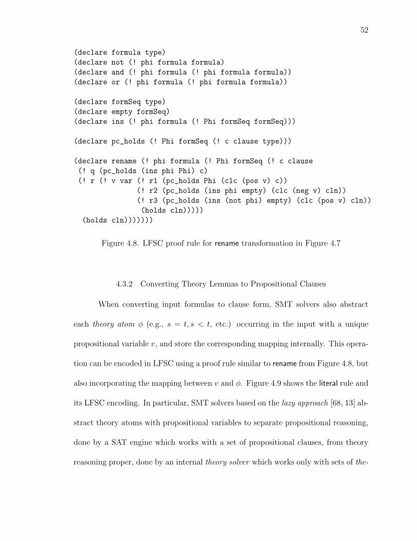
52
(declare formula type)
(declare not (! phi formula formula)
(declare and (! phi formula (! phi formula formula))
(declare or (! phi formula (! phi formula formula))
(declare formSeq type)
(declare empty formSeq)
(declare ins (! phi formula (! Phi formSeq formSeq)))
(declare pc_holds (! Phi formSeq (! c clause type)))
(declare rename (! phi formula (! Phi formSeq (! c clause
(! q (pc_holds (ins phi Phi) c)
(! r (! v var (! r1 (pc_holds Phi (clc (pos v) c))
(! r2 (pc_holds (ins phi empty) (clc (neg v) cln))
(! r3 (pc_holds (ins (not phi) empty) (clc (pos v) cln))
(holds cln)))))
(holds cln)))))))
Figure 4.8. LFSC proof rule for rename transformation in Figure 4.7
4.3.2 Converting Theory Lemmas to Propositional Clauses
When converting input formulas to clause form, SMT solvers also abstract
each theory atom φ (e.g., s = t, s < t, etc.) occurring in the input with a unique
propositional variable v, and store the corresponding mapping internally. This opera-
tion can be encoded in LFSC using a proof rule similar to rename from Figure 4.8, but
also incorporating the mapping between v and φ. Figure 4.9 shows the literal rule and
its LFSC encoding. In particular, SMT solvers based on the lazy approach [68, 13] ab-
stract theory atoms with propositional variables to separate propositional reasoning,
done by a SAT engine which works with a set of propositional clauses, from theory
reasoning proper, done by an internal theory solver which works only with sets of the-
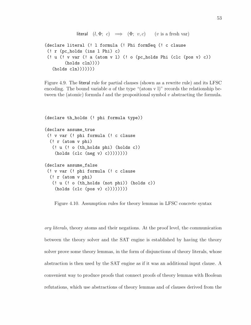
53
literal (l,Φ; c) =⇒ (Φ; v, c) (v is a fresh var)
(declare literal (! l formula (! Phi formSeq (! c clause
(! r (pc_holds (ins l Phi) c)
(! u (! v var (! a (atom v l) (! o (pc_holds Phi (clc (pos v) c))
(holds cln))))
(holds cln)))))))
Figure 4.9. The literal rule for partial clauses (shown as a rewrite rule) and its LFSCencoding. The bound variable a of the type “(atom v l)” records the relationship be-tween the (atomic) formula l and the propositional symbol v abstracting the formula.
(declare th_holds (! phi formula type))
(declare assume_true
(! v var (! phi formula (! c clause
(! r (atom v phi)
(! u (! o (th_holds phi) (holds c))
(holds (clc (neg v) c))))))))
(declare assume_false
(! v var (! phi formula (! c clause
(! r (atom v phi)
(! u (! o (th_holds (not phi)) (holds c))
(holds (clc (pos v) c))))))))
Figure 4.10. Assumption rules for theory lemmas in LFSC concrete syntax
ory literals, theory atoms and their negations. At the proof level, the communication
between the theory solver and the SAT engine is established by having the theory
solver prove some theory lemmas, in the form of disjunctions of theory literals, whose
abstraction is then used by the SAT engine as if it was an additional input clause. A
convenient way to produce proofs that connect proofs of theory lemmas with Boolean
refutations, which use abstractions of theory lemmas and of clauses derived from the
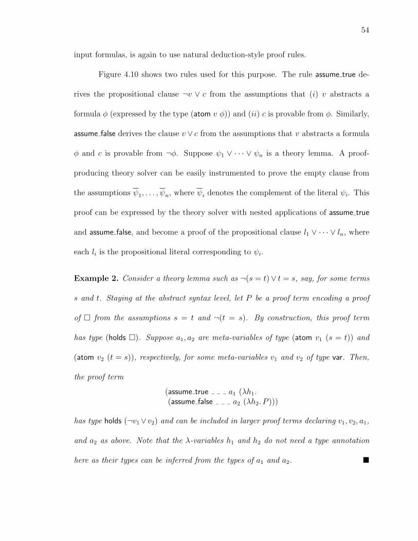
54
input formulas, is again to use natural deduction-style proof rules.
Figure 4.10 shows two rules used for this purpose. The rule assume true de-
rives the propositional clause ¬v ∨ c from the assumptions that (i) v abstracts a
formula φ (expressed by the type (atom v φ)) and (ii) c is provable from φ. Similarly,
assume false derives the clause v ∨ c from the assumptions that v abstracts a formula
φ and c is provable from ¬φ. Suppose ψ1 ∨ · · · ∨ ψn is a theory lemma. A proof-
producing theory solver can be easily instrumented to prove the empty clause from
the assumptions ψ1, . . . , ψn, where ψi denotes the complement of the literal ψi. This
proof can be expressed by the theory solver with nested applications of assume true
and assume false, and become a proof of the propositional clause l1 ∨ · · · ∨ ln, where
each li is the propositional literal corresponding to ψi.
Example 2. Consider a theory lemma such as ¬(s = t)∨ t = s, say, for some terms
s and t. Staying at the abstract syntax level, let P be a proof term encoding a proof
of from the assumptions s = t and ¬(t = s). By construction, this proof term
has type (holds ). Suppose a1, a2 are meta-variables of type (atom v1 (s = t)) and
(atom v2 (t = s)), respectively, for some meta-variables v1 and v2 of type var. Then,
the proof term
(assume true a1 (λh1.(assume false a2 (λh2. P )))
has type holds (¬v1∨v2) and can be included in larger proof terms declaring v1, v2, a1,
and a2 as above. Note that the λ-variables h1 and h2 do not need a type annotation
here as their types can be inferred from the types of a1 and a2.

55
x− x ≤ c c < 0 idl contra
x− y < c c− 1 = dx− y ≤ d
lt to leq
x− y ≤ a y − z ≤ b a+ b = cx− z ≤ c idl trans
Figure 4.11. Sample QF IDL rules and LFSC encodings. The variables x, y, z aredeclared SMT constant symbols and a, b, c, d are mpz numerals.
(declare int type) (declare as_int (! x mpz int))
(declare idl_contra (! x int (! c mpz
(! u (th_holds (<= (- x x) (as_int c))) (^ (ifneg c tt ff) tt)
(holds cln)))))
Figure 4.12. LFSC encoding of the idl contra rule. The as int builds a term of theSMT integer type int from a mpz number; tt and ff are the constructors of the bool
predefined type for Booleans.
4.3.3 Encoding Integer Difference Logic
The logic QF IDL, for quantifier-free integer difference logic, consists of for-
mulas interpreted over the integer numbers and restricted (in essence) to Boolean
combinations of atoms of the form x − y ≤ c where x and y are integer variables
(equivalently, free constants) and c is an integer value, i.e., a possibly negated nu-
meral. Some QF IDL rules for reasoning about the satisfiability of sets of literals in
this logic are shown in Figure 4.11, in conventional mathematical notation. Rule side
conditions are provided in braces, and are to be read as semantic expressions; for
example, a+ b = c in a side condition should be read as “c is the result of adding a
and b.” Note that the side conditions involve only values, and so can be checked by
(simple) computation. The actual language QF IDL contains additional atoms be-

56
sides those of the form of x− y ≤ c. For instance, atoms such as x < y and x− y ≥ c
are also allowed. Typical solvers for this logic use then a number of normalization
rules to reduce these additional atoms to the basic form. An example would be rule
lt to leq in Figure 4.11.
Encoding typical QF IDL proof rules in LFSC is straightforward thanks to
the built-in support for side conditions and for arbitrary precision integers in the side
condition language. As an example, Figure 4.12 shows the idl contra rule. Also, a
complete example QF IDL proof is explained in Appendix A.4.
4.4 Results for QF IDL Proof Checking
In this section we provide some empirical results on LFSC proof checking for
the logics presented in the previous section. These results were obtained with an
LFSC proof checker that we have developed to be both general (i.e., supporting the
whole LFSC language) and fast. The tool, which we will refer to as lfsc here, is
more accurately described as a proof checker generator : given an LFSC signature,
a text file declaring a proof system in LFSC format, it produces a checker for that
proof system. Some of its notable features in support of high performance proof
checking are the compilation of side conditions, as opposed to the incorporation of a
side condition language interpreter in the proof checker, and the generation of proof
checkers that check proof terms on the fly, as they parse them.
In separate work, we developed an SMT solver for the QF IDL logic, mostly to
experiment with proof generation in SMT. This solver, called clsat, can solve moder-
ately challenging QF IDL benchmarks from the SMT-LIB library, namely those clas-

57
sified with difficulty 0 through 3. 6 We ran clsat on the unsatisfiable QF IDL bench-
marks in SMT-LIB, and had it produce proofs in the LFSC proof system sketched in
Section 4.3.3 optimized with the deferred resolution rule described in Section 4.2.2.
Then we checked the proofs using the lfsc checker. The experiments were performed
on the SMT-EXEC solver execution service. 7 A timeout of 1,800 seconds was used
for each of the 622 benchmarks. 8 Table 4.1 summarizes those results for two configu-
rations: clsat (r453 on SMT-EXEC), in which clsat is run with proof-production off;
and clsat+lfsc (r591 on SMT-EXEC), in which clsat is run with proof-production
on, followed by a run of lfsc on the produced proof.
Table 4.1. Summary of results for QF IDL (timeout: 1,800 seconds)
Configuration Solved Unsolved Timeouts Time
clsat (without proofs) (r453) 542 50 30 29,507.7sclsat+lfsc (r591) 539 51 32 38,833.6s
The Solved column gives the number of benchmarks each configuration com-
pleted successfully. The Unsolved column gives the number of benchmarks each
configuration failed to solve before timeout due to clsat’s incomplete CNF conver-
sion implementation and lack of arbitrary precision arithmetic. The first configuration
6 The difficulty values of SMT benchmarks in SMT-LIB range from 0 to 5.
7 The results are publicly available at the SMT-EXEC service [6] under the job nameclsat-lfsc-2009.8.
8 The SMT-LIB library contains 692 benchmarks known to be unsatisfiable. 70 of themhave difficulty level 4 or 5, and are excluded in this experiment.

58
solved all benchmarks solved by the second. The one additional unsolved answer for
clsat+lfsc is diamonds.18.10.i.a.u.smt, the proof of which is bigger than 2GB in
size and the proof checker failed on due to a memory overflow. The Time column
gives the total times taken by each configuration to solve the 539 benchmarks solved
by both. Those totals show that the overall overhead of proof generation and proof
checking over just solving for those benchmarks was 31.6%, which we consider rather
reasonable.
For a more detailed picture on the overhead incurred with proof-checking,
Figure 4.13 compares proof checking times by clsat+lfsc with clsat’s solve-only times.
Each dot represents one of the 542 benchmarks that clsat could solve. The horizontal
axis is for solve-only times (without proof production) while the vertical axis is for
proof checking times. Both are in seconds on a log scale. It turned out that the
proofs from certain families of benchmarks, namely fischer, diamonds, planning
and post office, are much more difficult to verify than those for other families. In
particular, for those benchmarks proof checking took longer than solving. The worst
offender is benchmark diamonds.11.3.i.a.u.smt whose proof checking time was
2.30s vs 0.2s of solving time. However, the figure also shows that as these benchmarks
get more difficult, the relative proof overheads appear to converge towards 100%, as
indicated by the dotted line.9
9 The outlier above the dotted line is diamonds.18.10.i.a.u.smt.
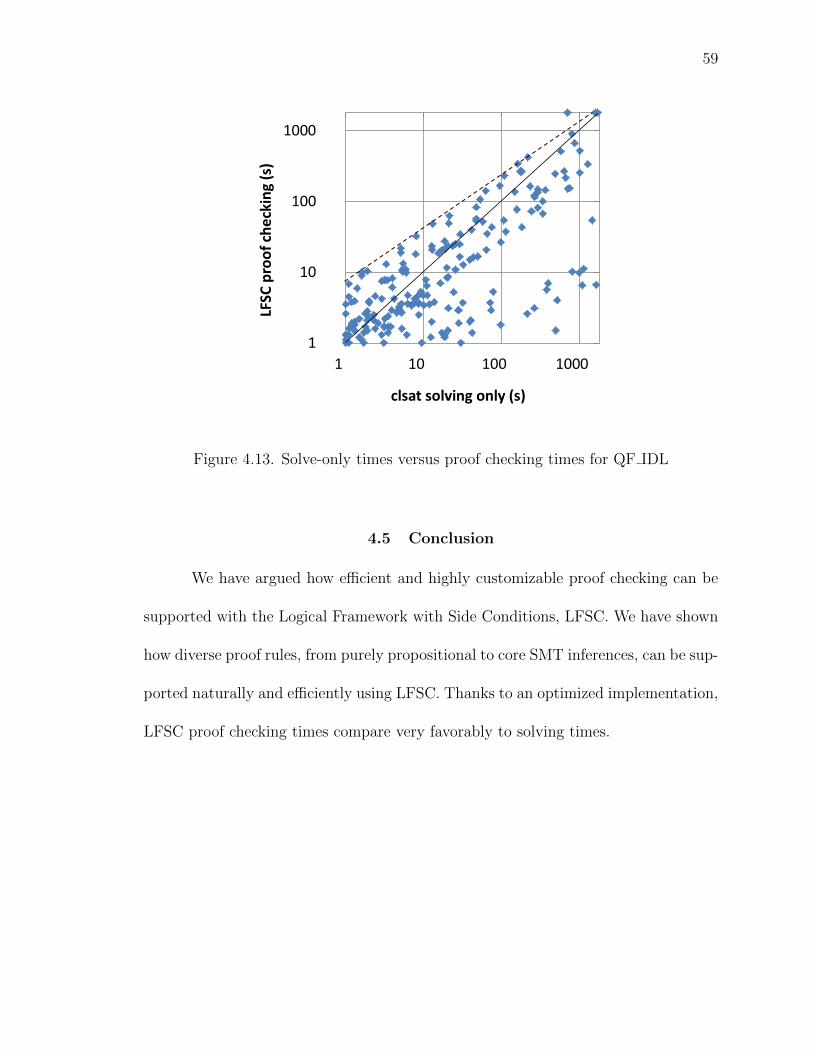
59
1
10
100
1000
1 10 100 1000
LFSC proof checking (s)
clsat solving only (s)
Figure 4.13. Solve-only times versus proof checking times for QF IDL
4.5 Conclusion
We have argued how efficient and highly customizable proof checking can be
supported with the Logical Framework with Side Conditions, LFSC. We have shown
how diverse proof rules, from purely propositional to core SMT inferences, can be sup-
ported naturally and efficiently using LFSC. Thanks to an optimized implementation,
LFSC proof checking times compare very favorably to solving times.

60
CHAPTER 5
VERIFYING MODERN SAT SOLVER USING DEPENDENT TYPES
In this chapter, we report on a verified modern SAT solver, called versat. The
versat program was written in a functional programming language, called Guru.
The Guru programming language is designed for verified programming by combin-
ing features of general programming languages and interactive theorem provers. Ver-
ifying SAT solver’s code requires a logic that is completely different from verifying
SAT/SMT proofs: a logic for general computations. Interactive theorem provers
have sought for logics for computation. Since Scott’s logic used λ-calculus to reason
about computation, functional programming languages have been used for defining
mathematical functions and used in many theorem provers. Beyond mathematics
and abstract algorithms, recent studies have applied interactive theorem provers to
verify complex properties of large software, such as compilers [50] and operating sys-
tems [47].
5.1 The Guru Programming Language
By way of background for the sections on the specification and implemen-
tation of versat below, we begin with a quick introduction to Guru. Guru is a
functional programming language with support for dependent types [12], inductive
data types [28], partial functions and resource types [73, 72]. Guru is inspired by
the Coq theorem prover for easy type-declaration with inductive data types and rich
expressiveness for describing strong software properties with dependent types. In ad-

61
dition to that, Guru allows for reasoning about partial functions (possibly diverging
computations), and efficient code generation by means of resource types.
Functional programming language. Guru is a functional programming lan-
guage, in which λ-abstraction (and µ-abstraction for recursive counterpart) is used
as the principle of function definition, and reductions (substitution of the λ/µ-bound
variables with a given term) as the principle of function application (call) and eval-
uation (computation). Reduction steps for applications of the λ and µ abstractions
are shown below:
(λx.t) u ⇒ [u/x]t(µf. t) u ⇒ [(µf. t)/f ]t u
The bracket expression [u/x]t means that every free occurrence of variable x of the
term t is replaced with the term u. The µ-abstraction above represents a recursive
function, in which the variable f represents the function itself. So, the reduction step
replicates the function in place of all the occurrences of f .
Like Coq, Guru supports inductive data types. An inductive data type defines
the symbols and grammar of terms that belong to the type. With inductive type
definitions, programs can pattern-match on first-order variables, which is essentially
the same as case-splitting on the possible top-level symbols of any term in place of
the variables.
Operational semantics. Guru has a deterministic operational semantics, namely
call-by-value (CBV, for short) semantics, in which function arguments are evaluated
first before the function is applied. Guru is a pure functional language in the sense

62
that program execution is not affected by any implicit states like memory content or
I/O states, other than the program term itself. Thus, any evaluations of the given
term always yields the same value.
Dependent types. As in the LFSC language, Guru is based on the λΠ-calculus
and supports dependent types. Π-abstracted types create type families indexed by
types (i.e. Πx : type. T [x]) or terms (i.e. Πx : T ′. T [x]), which are called polymorphic
and dependently typed, respectively. A type defines a set of terms/functions, and
various properties of terms and functions can be described using types. Dependent
type systems are very expressive, because one can use the same syntax for terms,
like inductive data types and pattern matching, to define types. So, dependent type
system brings together the language for terms and types.
Logic. The logic (the inference rules) of Guru is a first order logic with equality.
Guru provides a nice syntax for equality atoms and quantifiers (universal and exis-
tential). In addition to the usual reflexivity, transitivity and congruence rules, Guru
adds a provable equality over evaluation. A term is provably equal to the evaluated
term. 1 Thus, evaluating a term not only results in a value, but also admits the
fact that the term is equal to the resulting value. Guru’s induction rule allows for
reasoning about recursive functions by induction on the first-order input arguments
1 In fact, each step of evaluation is equal to the previous step, not just fully evaluatedterm. Thus, the sequence of evaluations is a chain of equal terms, just like simplificationsteps in Mathematics.
63
of functions. Note that every function argument is considered a finite value 2, which
is always true because function arguments are evaluated before their evaluated terms
(values) are passed to the function. 3
Partial functions. Unlike Coq, which systematically restricts all functions to be
total, Guru allows for general recursion (arbitrary µ-abstraction without any syn-
tactic restrictions). Thus, one can express looping (or diverging) terms and partial
functions. The advantage is that writing programs in Guru is easier than in Coq.
It is often very hard to show a function is total, which can be too costly for proto-
typing purposes and simple scripting needs. Also, termination may not be the most
important aspect of software, depending on the type of software. A SAT solver is a
good example: the SAT solver’s algorithm is terminating in theory; however, SAT
solvers are not expected to solve every formula in practice. Statistical evidence of the
performance will be more meaningful for this kind of software than the guarantee of
termination. On the other hand, partial functions make typing and inference rules
more complicated. Notably, indexed types and quantifier instantiations only allow
values (fully evaluated finite terms) to apply. Guru checks if each term being used
as an argument in such situations is indeed a value. One may prove a given term is
a value, using a termination proof. Also, a function may be proved to be total by
inductively showing that for all inputs, the function always returns a value. Once
2 A value is a term that cannot be evaluated any further
3 Because Guru supports partial function and the evaluation of term may not termi-nate, properties of functions are valid under the condition that their arguments are indeedterminating.

64
functions are proved to be total and registered with Guru, any applications of those
functions to values are automatically accepted as values. Thus, even though not re-
quired, it is often convenient to prove some functions to be total, especially, if they
are used in the context of types and proofs.
Resource types. Guru’s resource type system [72] is a separate typing system
from the regular type system mentioned above. It is a static analysis designed to
define resource (memory) management policies and direct the Guru compiler to
optimize the generated machine code. 4 One good example is a linear typing-like
policy with separate reader/writer references. With this policy, a memory object
can have at most one writer reference, and the object can be destructively updated
with the writer reference. Any number of reader references to the same object can
be created (for example, passing the object to other functions); however, the writer
reference will be locked until all the reader references are disposed. Such a policy is
encoded as a resource type in the Guru standard library, and prominently used in
versat to efficiently manage its data structures.
5.1.1 The Guru Syntax
In this section, we explain the Guru syntax by example. More detailed defi-
nition of the syntax is presented in Appendix B.1. Figure 5.1 shows the definitions of
natural numbers (Peano numbers) as an inductive type, and the isZ and plus function
4 Guru compiles programs into the C programming language, and then into the machinecode by a standard C compiler. Guru also features some basic optimizations including tail-recursion.
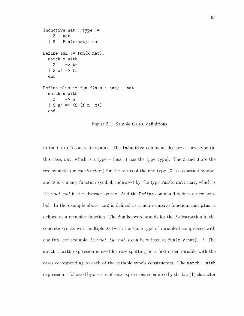
65
Inductive nat : type :=
Z : nat
| S : Fun(x:nat). nat
Define isZ := fun(x:nat).
match x with
Z => tt
| S x’ => ff
end
Define plus := fun f(n m : nat) : nat.
match n with
Z => m
| S n’ => (S (f n’ m))
end
Figure 5.1. Sample Guru definitions
in the Guru’s concreate syntax. The Inductive command declares a new type (in
this case, nat, which is a type – thus, it has the type type). The Z and S are the
two symbols (or constructors) for the terms of the nat type. Z is a constant symbol
and S is a unary function symbol, indicated by the type Fun(x:nat).nat, which is
Πx : nat. nat in the abstract syntax. And the Define command defines a new sym-
bol. In the example above, isZ is defined as a non-recursive function, and plus is
defined as a recursive function. The fun keyword stands for the λ-abstraction in the
concrete syntax with multiple λs (with the same type of variables) compressed with
one fun. For example, λx : nat. λy : nat. t can be written as fun(x y:nat). t . The
match. . . with expression is used for case-splitting on a first-order variable with the
cases corresponding to each of the variable type’s constructors. The match. . . with
expression is followed by a series of case-expressions separated by the bar (|) character

66
and the end keyword. Each case starts with a constructor symbol. If the constructor
has a function type, variables representing the arguments to the constructor should
follow the constructor symbol. The arguments to constructors are also called subdata
of the term being matched on (or the scrutinee). Then, an arrow symbol (=>) and
the subprogram for the case follow. The constructors tt and ff are for the bool
(Boolean) type, defined in the Guru standard library. For recursive functions, a
name follows the fun keyword (like f for the plus definition), and the return type of
the function should be stated (like : nat for plus), which is necessary for decidable
type checking. The name following fun is the µ bound variable and used for the
recursive reference of the function itself. Finally, function applications t u are written
as (t u), where parentheses are strictly required. Also, type-level applications are
written as <t u>, where the type of t is a Π-abstraction.
5.1.2 Verified Programming in Guru
In Guru, programs can be verified both externally (as in traditional theorem
provers), and internally (cf [9]). For a standard example of the difference, suppose
we wish to prove that the result of appending two lists has length equal to the sum
of the input lengths.
External verification of this property may proceed like this. First, we define
the type of append function on lists. In Guru syntax, the typing for this append
function is:
append : Fun(A:type)(l1 l2 : <list A>). <list A>
This says that append accepts a type A, and lists l1 and l2 holding elements of type

67
A, and produces another such list. To verify the desired property, we write a proof in
Guru’s proof syntax of the following formula:
Forall(A:type)(l1 l2:<list A>).
(length (append l1 l2)) = (plus (length l1) (length l2))
The equality listed expresses, in Guru’s semantics, that the term on the left-hand
side evaluates to the same value as the term on the right-hand side. So the formula
states that for all types A, for all lists l1 and l2 holding elements of that type, calling
the length function on the result of appending l1 and l2 gives the same result as
adding the lengths of l1 and l2. This is the external approach.
With internal verification, we first define an alternative indexed datatype for
lists. A type index is a program value occurring in the type, in this case the length
of the list. We define the type <vec A n> to be the type of lists storing elements of
type A, and having length n, where n is a natural number:
Inductive vec : Fun(A:type)(n:nat).type :=
vecn : Fun(A:type). <vec A Z>
| vecc : Fun(A:type)(spec n:nat)(a:A)(l:<vec A n>). <vec A (S n)>
This states that vec is inductively defined with constructors vecn and vecc (for nil
and cons, respectively). The return type of vecc is <vec A (S n)>, where S is the
successor function. So the length of the list returned by the constructor vecc is one
greater than the length of the sublist l. Note that the argument n (of vecc) is labeled
“spec”, which means specificational. Guru will enforce that no run-time results will
depend on the value of this argument, thus enabling the compiler to erase all values
for that parameter in compiled code.
We can now define the type of vec append function on vectors:

68
vec_append : Fun(A:type)(spec n m:nat)
(l1:<vec A n>)(l2:<vec A m>). <vec A (plus n m)>
This type states that append takes in a type A, two specificational natural numbers n
and m, and vectors l1 and l2 of the corresponding lengths, and returns a new vector
of length (plus n m). This is how internal verification expresses the relationship
between lengths which we proved externally above. Type-checking code like this may
require the programmer to prove that two types are equivalent. For example, a proof
of commutativity of addition is needed to prove <vec A (plus n m)> equivalent
to <vec A (plus m n)>. Currently, these proofs must mostly be written by the
programmer, using special proof syntax, including syntax for inductive proofs.
5.2 Formalizing Correct SAT Solvers
The main property of versat is the soundness of the solver on top of the
basic requirements of Guru, such as memory safety and array-bounds checking. We
encoded the underlying logic of SAT in Guru to reason about the behavior of the
SAT solver. That encoding includes the representation of formulas and the deduction
rules. For a “UNSAT” answer, our specification requires that there exists a derivation
proof of the empty clause from the input formula. Note that most solvers can generate
a model with a “SAT” answer and those models can be checked very efficiently. So,
we do not think there is a practical advantage for statically verifying the soundness
of “SAT” answers. Also, it is important to note that the specification is the only part
we need to trust. So, it should be clear and concise. The specification of versat is
only 259 lines of Guru code. The rest of versat is the actual implementation and
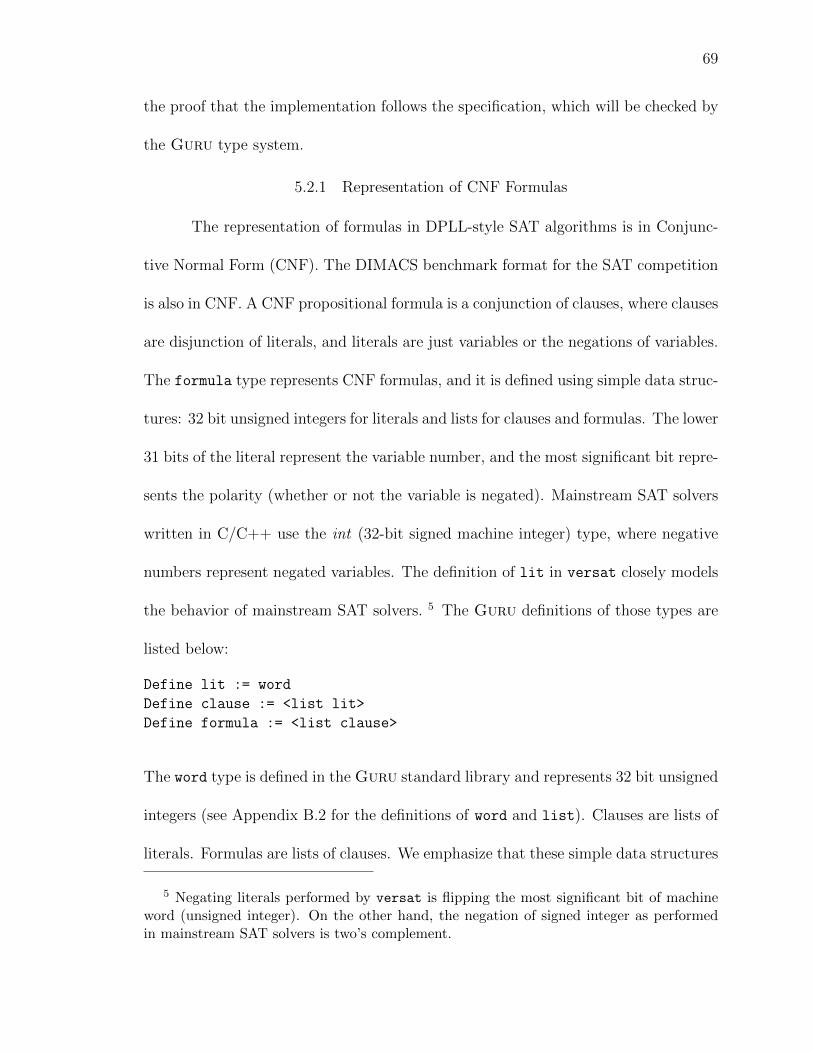
69
the proof that the implementation follows the specification, which will be checked by
the Guru type system.
5.2.1 Representation of CNF Formulas
The representation of formulas in DPLL-style SAT algorithms is in Conjunc-
tive Normal Form (CNF). The DIMACS benchmark format for the SAT competition
is also in CNF. A CNF propositional formula is a conjunction of clauses, where clauses
are disjunction of literals, and literals are just variables or the negations of variables.
The formula type represents CNF formulas, and it is defined using simple data struc-
tures: 32 bit unsigned integers for literals and lists for clauses and formulas. The lower
31 bits of the literal represent the variable number, and the most significant bit repre-
sents the polarity (whether or not the variable is negated). Mainstream SAT solvers
written in C/C++ use the int (32-bit signed machine integer) type, where negative
numbers represent negated variables. The definition of lit in versat closely models
the behavior of mainstream SAT solvers. 5 The Guru definitions of those types are
listed below:
Define lit := word
Define clause := <list lit>
Define formula := <list clause>
The word type is defined in the Guru standard library and represents 32 bit unsigned
integers (see Appendix B.2 for the definitions of word and list). Clauses are lists of
literals. Formulas are lists of clauses. We emphasize that these simple data structures
5 Negating literals performed by versat is flipping the most significant bit of machineword (unsigned integer). On the other hand, the negation of signed integer as performedin mainstream SAT solvers is two’s complement.
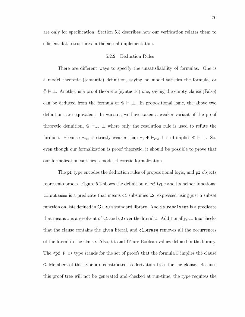
70
are only for specification. Section 5.3 describes how our verification relates them to
efficient data structures in the actual implementation.
5.2.2 Deduction Rules
There are different ways to specify the unsatisfiability of formulas. One is
a model theoretic (semantic) definition, saying no model satisfies the formula, or
Φ ⊥. Another is a proof theoretic (syntactic) one, saying the empty clause (False)
can be deduced from the formula or Φ ` ⊥. In propositional logic, the above two
definitions are equivalent. In versat, we have taken a weaker variant of the proof
theoretic definition, Φ `res ⊥ where only the resolution rule is used to refute the
formula. Because `res is strictly weaker than `, Φ `res ⊥ still implies Φ ⊥. So,
even though our formalization is proof theoretic, it should be possible to prove that
our formalization satisfies a model theoretic formalization.
The pf type encodes the deduction rules of propositional logic, and pf objects
represents proofs. Figure 5.2 shows the definition of pf type and its helper functions.
cl subsume is a predicate that means c1 subsumes c2, expressed using just a subset
function on lists defined in Guru’s standard library. And is resolvent is a predicate
that means r is a resolvent of c1 and c2 over the literal l. Additionally, cl has checks
that the clause contains the given literal, and cl erase removes all the occurrences
of the literal in the clause. Also, tt and ff are Boolean values defined in the library.
The <pf F C> type stands for the set of proofs that the formula F implies the clause
C. Members of this type are constructed as derivation trees for the clause. Because
this proof tree will not be generated and checked at run-time, the type requires the

71
Define eq_lit := eqword
Define eq_clause := (eqlist lit eqword)
Define cl_has := fun(c:clause)(l:lit). (member lit l c eq_lit)
Define cl_erase := fun(c:clause)(l:lit). (erase lit eq_lit l c)
Define cl_subsume := fun(c1:clause)(c2:clause).
(list_subset lit eq_lit c1 c2)
Define is_resolvent := fun(r:clause)(c1:clause)(c2:clause)(l:lit).
(and (and (cl_has c1 (negated l))
(cl_has c2 l))
(and (cl_subsume (cl_erase c1 (negated l)) r)
(cl_subsume (cl_erase c2 l) r)))
Inductive pf : Fun(F : formula)(C : clause).type :=
pf_asm : Fun(F : formula)(C:clause)
(u : (member C F eq_clause) = tt ). <pf F C>
| pf_sub : Fun(F : formula)(C C’ : clause)
(d : <pf F C’>)
(u : (cl_subsume C’ C) = tt ). <pf F C>
| pf_res : Fun(F : formula)(C C1 C2 : clause)(l : lit)
(d1 : <pf F C1>)(d2 : <pf F C2>)
(u : (is_resolvent C C1 C2 l) = tt ). <pf F C>
Figure 5.2. Encoding of the inference system (pf) and its helper functions
proper preconditions at each constructor. Guru’s type system ensures that those
proof objects are valid by construction.
The eqword, member, and erase functions are defined in the Guru standard
library (see Appendix B.2 for their definitions). The pf asm constructor stands for the
assumption rule, which proves any clause in the input formula. The member function
looks for the clause C in the formula, returning tt if so. The pf sub constructor
stands for the subsumption rule. This rule allows to remove duplicated literals or
change the order of literals in a proven clause. Note that the constructor requires a
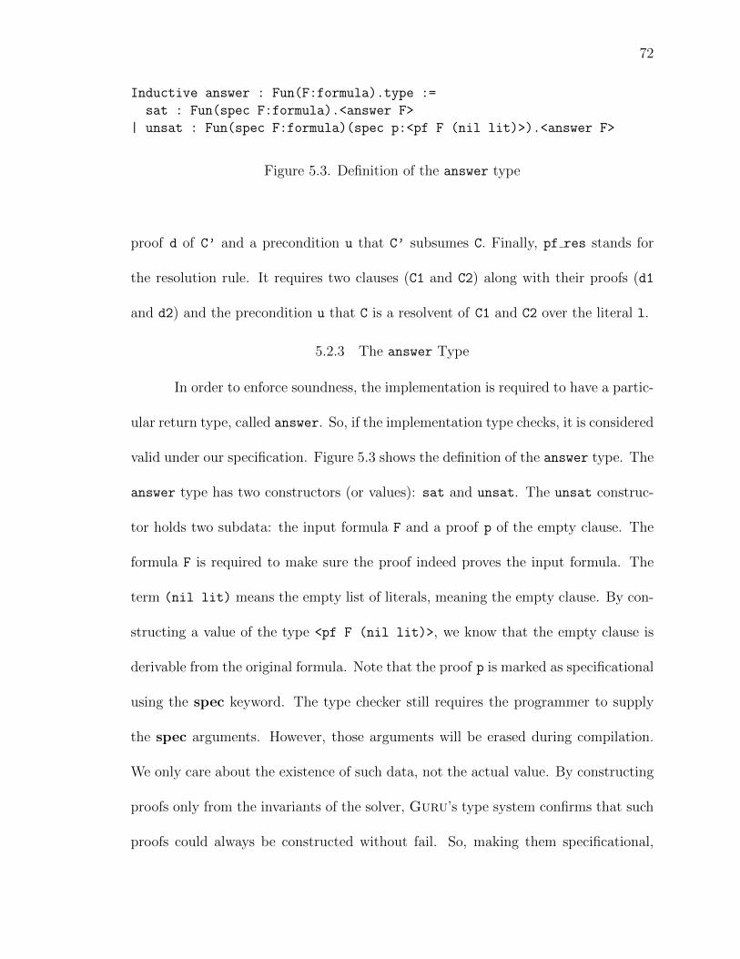
72
Inductive answer : Fun(F:formula).type :=
sat : Fun(spec F:formula).<answer F>
| unsat : Fun(spec F:formula)(spec p:<pf F (nil lit)>).<answer F>
Figure 5.3. Definition of the answer type
proof d of C’ and a precondition u that C’ subsumes C. Finally, pf res stands for
the resolution rule. It requires two clauses (C1 and C2) along with their proofs (d1
and d2) and the precondition u that C is a resolvent of C1 and C2 over the literal l.
5.2.3 The answer Type
In order to enforce soundness, the implementation is required to have a partic-
ular return type, called answer. So, if the implementation type checks, it is considered
valid under our specification. Figure 5.3 shows the definition of the answer type. The
answer type has two constructors (or values): sat and unsat. The unsat construc-
tor holds two subdata: the input formula F and a proof p of the empty clause. The
formula F is required to make sure the proof indeed proves the input formula. The
term (nil lit) means the empty list of literals, meaning the empty clause. By con-
structing a value of the type <pf F (nil lit)>, we know that the empty clause is
derivable from the original formula. Note that the proof p is marked as specificational
using the spec keyword. The type checker still requires the programmer to supply
the spec arguments. However, those arguments will be erased during compilation.
We only care about the existence of such data, not the actual value. By constructing
proofs only from the invariants of the solver, Guru’s type system confirms that such
proofs could always be constructed without fail. So, making them specificational,
73
hence not computing them at run-time, is sound. Now, the typing of the SAT solver
implementation, solve using the answer type is following:
solve : Fun(nv:word)(F:formula). <answer F>
The extra argument nv stands for the number of variables in the formula, which is
stated in the given DIMACS benchmark file. This number is used for determining
the size of various data structures such as look-up tables in versat. Also, note that
the dependent typing makes sure that the formula that the answer type is talking
about is indeed the input formula, not just any formula.
5.2.4 Parser and Entry Point
The formula type above is still in terms of integer and list data structures, not
a stream of characters as stored in a benchmark file. The benchmark file has to be
translated to Guru data structure before it can be reasoned about. So, we include a
simple recursive parser for the DIMACS standard benchmark format, which amounts
to 145 lines of Guru code, as a part of our specification. It might be possible to
reduce this using a verified parser generator, but we judge there to be more important
targets of further verification. Similarly, the main function is considered a part of the
specification, as the outcome of the solve function is an answer value, not the action
of printing ”SAT” or ”UNSAT”. The main function simply calls the parser, passes
the output to the solve function, and prints the answer as a string of characters.

74
5.3 Implementation and Invariants
The specification in Section 5.2 does not constrain the details of the imple-
mentation very much. For a trivial example, a solver that just aborted immediately
on every input formula would satisfy the specification. So would a solver that used
the naive data structures for formulas, or a naive solving algorithm. Therefore, we
have imposed an additional informal constraint on versat, which is that it should
use efficient low-level data structures, and should implement a number of the essen-
tial features of modern SAT solvers. The features implemented in versat are conflict
analysis, clause learning, backjumping, watched literals, and basic decision heuristics.
Also, each of these features is implemented using the same efficient data structures
that can be found in a C-language implementation like tinisat or minisat. How-
ever, implementing more features and optimizations make it more difficult to prove
the soundness property.
Modern SAT solvers are driven by conflict analysis, during which a new clause
is deduced and recorded to guide the search. Thus, the critical component for sound-
ness is the conflict analysis module, which can be verified, to some extent, in isolation
from the rest of the solver. Verifying that every learned clause is a consequence of
the input clauses ensures the correctness of UNSAT answers from the solver, in the
special case of the empty clause. Using the internal-verification approach described
in the previous section, the conflict analysis module enforces soundness by requiring
that with each learned clause added to the clause database, there is an accompanying
specificational proof (the pf datatype described in Section 5.2). In this section, we

75
Inductive aclause : Fun(nv:word)(F:formula).type :=
mk_aclause : Fun(spec n:word)(l:<array lit n>)
(spec nv:word)(spec F:formula)
(u1: (array_in_bounds nv l) = tt )
(spec c:clause)(spec pf_c:<pf F c>)
(u2: c = (to_cl l) ).
<aclause nv F>
Figure 5.4. Definition of the array-based clauses and invariants (aclause)
explain some of the run-time clause data structure along with the invariants, and the
conflict analysis implementation.
5.3.1 Array-based Clauses and Invariants
In the specification, the data structure for clauses is (singly linked) list, which
is straightforward to reason about. However, accessing elements in a list is not as
efficient as an array. The elements of an array are more likely in the same cache line,
which leads to a faster sequential access, as elements in a linked list are not. Also
arrays will use less memory than lists because of the extra storage for pointers. So, at
the implementation level, versat uses array-based clauses with invariants as defined
in Figure 5.4. An <array lit n> object stands for an array of literals of size n, where
n has the type word. The variable nv represents the number of different variables in
the formula F. It is also the maximum possible value for variable numbers as defined
in the DIMACS file format (variables are named from 1 up to nv). The predicate
(array in bounds nv l) used in the invariant u1 means every variable in the array
l is less than or equal to nv and not equal to zero. The invariant u1 is used to avoid
run-time checks for array bounds when accessing a number of look-up tables indexed
76
by the variable number, such as the current assignment value, the reference to the
antecedent clauses, and the decision level for a given variable.
The array l is implicitly null-terminated. The word value zero (the null literal)
is used as the termination marker of a given array. The null literal should be present
within the bounds of the array, and only the literals up to the null literal make up
the clause. 6 Null-terminated arrays are used in most of mainstream SAT solvers
to store clauses for simplicity and performance of accessing clauses. By having an
array null-terminated, the end of the array can be detected during sequential access,
without a separate variable storing the length of the array. Note that the variable
n is marked as specification, so the length of the array l is not traced at runtime.
Interestingly, the null-termination property of the array l is implied by the invariant
u1. The array_in_bounds function is a partial function that returns a boolean value
only for properly null-terminated arrays; otherwise, the return values is undefined.
Thus, from the invariant u1, which states that the function returned the tt value,
it can be proved that the array l is null-terminated.7 The difficulty of using a null-
terminated array is that we need to prove array accesses up to the null literal are
indeed within bounds of the array. The following lemma (proved in Guru) states
that if an array-based clause has the invariant u1, its length is strictly greater than
zero.
6 The rest of the array after the null literal is ignored, if any. In fact, versat alwaysallocate an array just big enough to contain the clause and the null literal.
7 In fact, the null-termination is also implied by u2 as well, because the to cl functionis a partial function only defined for null-terminated arrays.
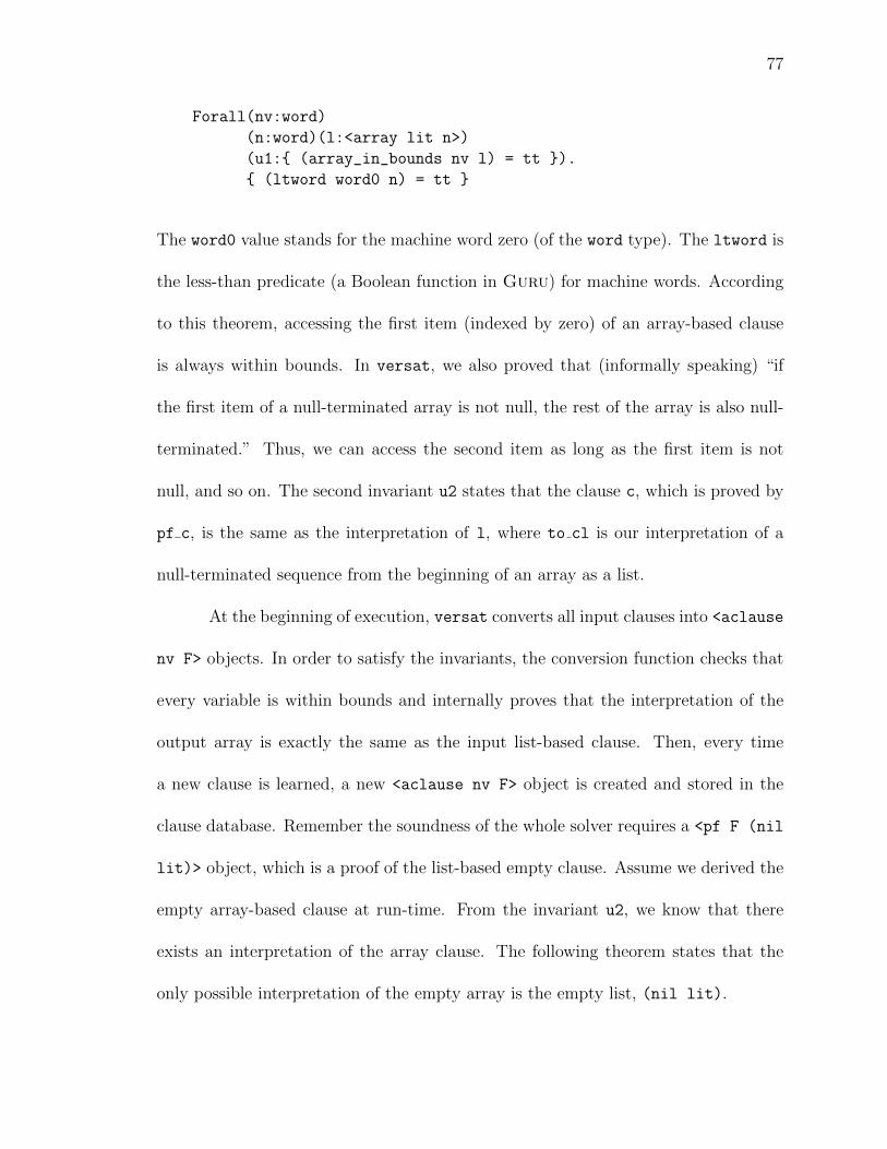
77
Forall(nv:word)
(n:word)(l:<array lit n>)
(u1: (array_in_bounds nv l) = tt ).
(ltword word0 n) = tt
The word0 value stands for the machine word zero (of the word type). The ltword is
the less-than predicate (a Boolean function in Guru) for machine words. According
to this theorem, accessing the first item (indexed by zero) of an array-based clause
is always within bounds. In versat, we also proved that (informally speaking) “if
the first item of a null-terminated array is not null, the rest of the array is also null-
terminated.” Thus, we can access the second item as long as the first item is not
null, and so on. The second invariant u2 states that the clause c, which is proved by
pf c, is the same as the interpretation of l, where to cl is our interpretation of a
null-terminated sequence from the beginning of an array as a list.
At the beginning of execution, versat converts all input clauses into <aclause
nv F> objects. In order to satisfy the invariants, the conversion function checks that
every variable is within bounds and internally proves that the interpretation of the
output array is exactly the same as the input list-based clause. Then, every time
a new clause is learned, a new <aclause nv F> object is created and stored in the
clause database. Remember the soundness of the whole solver requires a <pf F (nil
lit)> object, which is a proof of the list-based empty clause. Assume we derived the
empty array-based clause at run-time. From the invariant u2, we know that there
exists an interpretation of the array clause. The following theorem states that the
only possible interpretation of the empty array is the empty list, (nil lit).
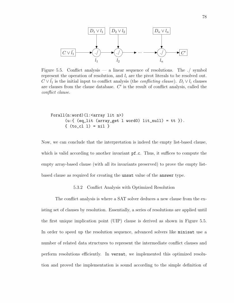
78
C ∨ l1
D1 ∨ l1
./
l1
D2 ∨ l2
./
l2
...
Dn ∨ ln
./
ln
C ′
Figure 5.5. Conflict analysis — a linear sequence of resolutions. The ./ symbolrepresent the operation of resolution, and li are the pivot literals to be resolved out.C ∨ l1 is the initial input to conflict analysis (the conflicting clause). Di ∨ li clausesare clauses from the clause database. C ′ is the result of conflict analysis, called theconflict clause.
Forall(n:word)(l:<array lit n>)
(u: (eq_lit (array_get l word0) lit_null) = tt ).
(to_cl l) = nil
Now, we can conclude that the interpretation is indeed the empty list-based clause,
which is valid according to another invariant pf c. Thus, it suffices to compute the
empty array-based clause (with all its invariants preserved) to prove the empty list-
based clause as required for creating the unsat value of the answer type.
5.3.2 Conflict Analysis with Optimized Resolution
The conflict analysis is where a SAT solver deduces a new clause from the ex-
isting set of clauses by resolution. Essentially, a series of resolutions are applied until
the first unique implication point (UIP) clause is derived as shown in Figure 5.5.
In order to speed up the resolution sequence, advanced solvers like minisat use a
number of related data structures to represent the intermediate conflict clauses and
perform resolutions efficiently. In versat, we implemented this optimized resolu-
tion and proved the implementation is sound according to the simple definition of

79
¬lC lD
n m
./
l
C ′
Figure 5.6. Naive implementation of resolution. The resolvent C ′ is computed bycopying the literals from C except for ¬l and copying the literals from D except forl. n and m are the lengths of C and D. The time complexity is linear in n+m.
is resolvent in the specification.
Figure 5.6 shows a naive implementation of resolvent computation. The time
complexity of this implementation is linear in the lengths of the two input clauses,
O(n + m). Mainstream SAT solvers improve the time complexity to O(m) using a
combination of techniques. In addition to the speed-up, we want to avoid duplicated
literals in the resolvent C ′. Otherwise, the result of conflict analysis will contain many
duplicate literals, which take up memory space and processing time. Duplication
removal can be easily achieved by using a look-up table shown in Figure 5.7. The
look-up table L indexes the content of C ′, and effectively duplicates the content of of
C ′ in a different layout in memory. 8 Whenever a literal is inserted to the resolvent
C ′, we use the table L to see if the literal is already present in C ′, so that we can
avoid adding duplicate literals to C ′. To prove this resolvent computation is correct,
8 Indirection(indexing) and duplication are common in many software engineering tech-niques.
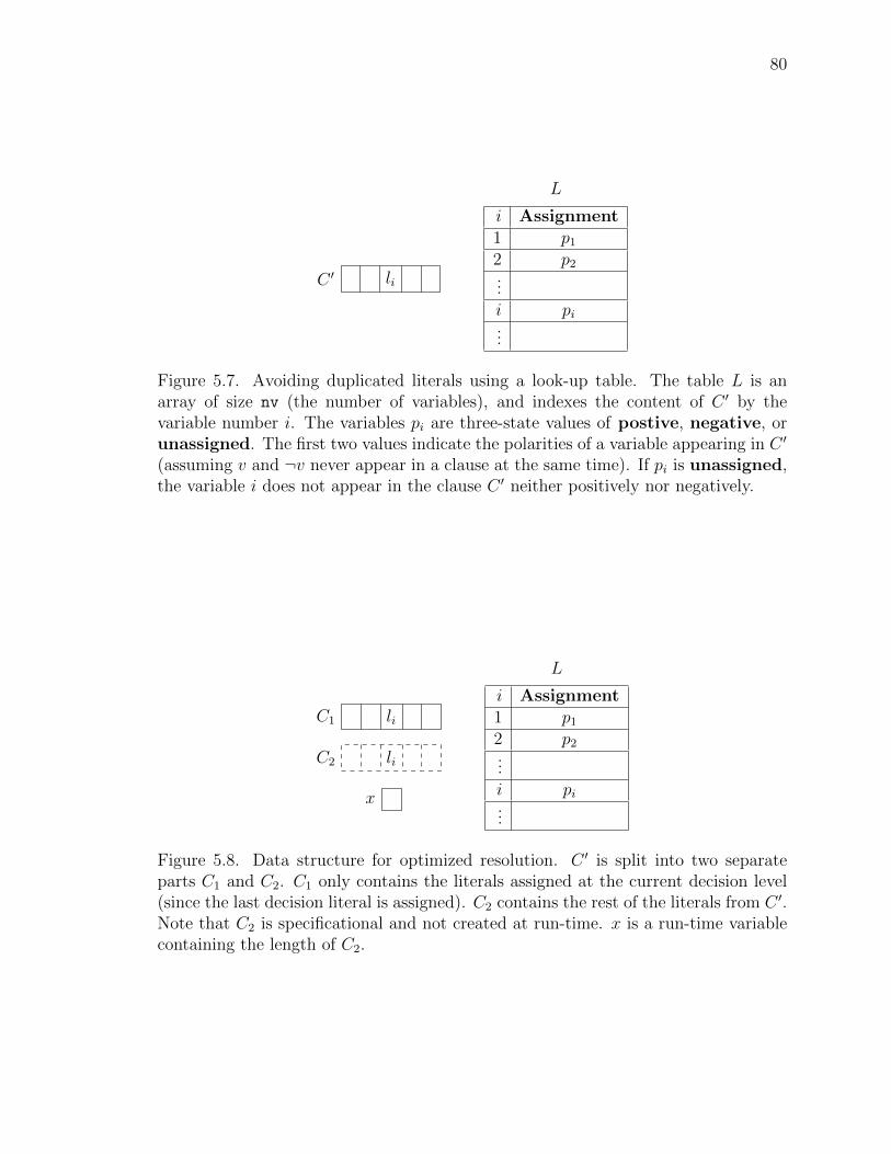
80
liC ′
i Assignment1 p12 p2...i pi...
L
Figure 5.7. Avoiding duplicated literals using a look-up table. The table L is anarray of size nv (the number of variables), and indexes the content of C ′ by thevariable number i. The variables pi are three-state values of postive, negative, orunassigned. The first two values indicate the polarities of a variable appearing in C ′
(assuming v and ¬v never appear in a clause at the same time). If pi is unassigned,the variable i does not appear in the clause C ′ neither positively nor negatively.
liC1
liC2
x
i Assignment1 p12 p2...i pi...
L
Figure 5.8. Data structure for optimized resolution. C ′ is split into two separateparts C1 and C2. C1 only contains the literals assigned at the current decision level(since the last decision literal is assigned). C2 contains the rest of the literals from C ′.Note that C2 is specificational and not created at run-time. x is a run-time variablecontaining the length of C2.

81
we need an invariant that the contents of C ′ and L are coherent. An important
property of conflict analysis is that the pivot literals (in Figure 5.5) are always the
literals that are assigned after the last decision literal. When a SAT solver explores
the search space finding a model, it incrementally build partial models by asserting
certain literals. There are two different kinds of asserted literals: decision literals and
deduced literals. Decision literals are speculatively asserted literals by the SAT solver
to find a candidate model. Deduced literals are asserted because they are inferred
from the input formula and the other asserted literals. In other words, conflict analysis
is a procedure to resolve out the literals asserted since the last decision. That means
the SAT solver knows which literals may be removed during conflict analysis at the
beginning. Using this property, we can achieve the improved complexity of O(m).
Figure 5.8 shows the abstract data structure for the optimized resolution. This
data structure represents intermediate clauses deduced by resolution steps. Also, the
data structure is reused for the next resolution by destructively updating it, instead
of creating a new one. In this version, C ′ is split into C1 and C2. C1 contains the
literals assigned before the last decision, C2 contains the rest of C ′. Only the literals
in C2 may be removed during conflict analysis, and C1 will only grow. Note that C2
is specificational data and not created at run-time. Instead, a new run-time variable
x keeps track of the supposed length of C2. The length of C2 is used to check for early
termination of conflict analysis. Conflict analysis terminates when it deduces the first
UIP clause. A UIP clause has only one literal assigned since the last decision. Thus,
as soon as the length of C2 becomes 1 at the end of resolution, conflict analysis stops.

82
That is the reason why we monitor the length of C2, even though we do not need the
content of C2 at run-time.
Figure 5.9 shows the concrete data structure ResState representing interme-
diate conflict clauses and their invariants, which are maintained after each resolution
step over the course of conflict analysis. Those invariants are sufficient to prove the
soundness of versat’s conflict analysis. Table 5.1 summarizes the variables used in
the ResState type. The conflict clause is split into the literals assigned at the pre-
vious decision levels (c1) and the literals assigned at the current level (c2) according
to the invariant u5. So, the complete conflict clause at the time is (append c1 c2).
Notice that c2 is declared as a specificational data with the spec keyword. Dur-
ing conflict analysis, versat does not build each intermediate conflict clause as a
single complete clause. Instead, the whole conflict clause is duplicated in a look-up
table (vt), and it keeps track of the number of literals assigned at the current level,
which is the c2l, as stated by the invariants u1, u2 and u3. The u2 and u3 ensure
that the conflict clause and the table contain exactly the same set of literals. The
look-up table vt enables a constant time check whether a literal is in the conflict
clause, which makes duplication removal and other operations efficient. And it also
enables a constant time removal of a literal assigned at the current level, which can
be done by unmarking the literal on the vt and decrementing the value of c2l by
one. That also requires all literals in the list c2 to be distinct (u4), so that removing
all occurrences of a literal (as in the specification) will decrease the length only by
one (in the implementation). Note that, although the type of c2l is nat (the Peano

83
Inductive ResState : Fun(nv:word)(dl:word).type :=
res_state : Fun
(spec nv:word)
(spec dl:word)
(dls:<array word nv>)
(vt:<array assignment nv>)
(c1:clause)
(spec c2:clause)
(c2l:nat)
(u1: c2l = (length c2) )
(u2: (all_lits_are_assigned vt (append c2 c1)) = tt )
(u3: (cl_has_all_vars (append c2 c1) vt) = tt )
(u4: (cl_unique c2) = tt )
(u5: (cl_set_at_prev_levels dl dls c1) = tt )
.<ResState nv dl>
Figure 5.9. Definition of conflict analysis state (ResState)
number), incrementing/decrementing by one and zero testing are constant time op-
erations just like the machine integer operations. Also, note that, some invariants —
e.g. all variables are within bounds — are omitted in the figure for clarity.
For the resolution function, we have proved that the computation of the re-
solvent between the previous conflict clause and the antecedent clause follows the
specification of is resolvent, so that a new pf object for the resolvent can be con-
structed. At the end of the conflict analysis, versat will find the Unique Implication
Point (UIP) literal, say l, and the ResState value will have one as the value of c2l.
Because the UIP literal must be assigned at the current decision level, it should be in
c2 and the length of c2 is one due to the invariant u1. That means actually c2 is a sin-
gleton list that consists of l. Thus, the complete conflict clause is (cons lit l c1).
Then, an array-base clause can be constructed and stored in the clause database, just

84
Table 5.1. Summary of variables used in ResState
Var Description
nv the number of variables in the formuladl the current decision leveldls a table of the decision levels at which each variable is assignedvt a look-up table for the variables in the conflict clausec1 the literals of the conflict clause assigned at the previous decision levelsc2 the literals of the conflict clause assigned at the current decision levelc2l the length of c2u1 the length of the list c2 is the same as the value of c2lu2 all the literals in the conflict clause are marked on the tableu3 all the literals marked on the table are in the conflict clauseu4 all literals in the list c2 are uniqueu5 all variables in c1 are assigned at the previous decision levels
as the input list-based clauses are processed at the beginning of execution. Finally,
versat clears up the table vt by unmarking all the literals to recycle for the next
analysis. Instead of sweeping through the whole table, versat only unmarks those
literals in the conflict clause. It can be proved that after unmarking those literals,
the table is clean as new using the invariant u3 above. Correctness of this clean-up
process is proved in around 400 lines of lemmas, culminating in the theorem in Fig-
ure 5.10, which states that the efficient table-clearing code (clear_vars) returns a
table which is indistinguishable from a brand new array (created with array_new).
5.3.3 Summary of Implementation
The source code of versat totals 9884 lines, including proofs. It is hard to
separate proofs from code because they can be intermixed within a function. Roughly
speaking, auxiliary code (to formulate invariants) and proofs take up 80% of the entire
program. The generated C code weighs in at 12712 lines. The C code is self-contained

85
Forall (nv:word)
(vt:<array assignment nv>)
(c:clause)
(u: (cl_valid nv c) = tt )
(r: (cl_has_all_vars c vt) = tt )
. (clear_vars vt c) = (array_new nv UN)
Figure 5.10. Correctness theorem for table-clearing code
and includes the translations of Guru’s library functions being used. All lemmas used
by versat have been machine-checked by the Guru compiler.
Properties not proved. First, we do not prove termination for versat. It
could (a priori) be the case that the solver diverges on some inputs, and it could
also be the case that certain run-time checks we perform (discussed in Section 5.5)
fail. These termination properties have not been formally verified. However, what
users want is to solve problems in a reasonable amount of time. A guarantee of
termination does not satisfy users’ expectations. It is more important to evaluate
the performance over real problems as we show in Section 5.4. Second, we have not
verified completeness of versat. It is (again a priori) possible that versat reports
satisfiable, but the formula is actually unsatisfiable. In fact, we include a run-time
check at the end of execution, to ensure that when versat reports SAT, the formula
does have a model. But it would take substantial additional verification to ensure
that this run-time check never fails.

86
5.4 Results: versat Performance
We compared versat to picosat-936 with proof generation and checking
for certified UNSAT answers. picosat [19] is one of the best SAT solvers and can
generate proofs in the RUP and TraceCheck formats. The RUP proof format [75] is
the official format for the certified track of the SAT competition, and checker3 is
used as the trusted proof checker. The TraceCheck format [7] is picosat’s preferred
proof format, and the format and checker are made by the developers of picosat.
We measured the runtime of the whole workflow of solving, proof generation, and
checking in both of the formats over the benchmarks used for the certified track of
the SAT competition 2007. The certified track has not been updated since then.
Table 5.2 shows the performance comparison. The “versat” column shows the
solving times of versat. The “picosat(R)” and “picosat(T)” columns shows the solv-
ing and proof generation times of picosat in the RUP format and TraceCheck format,
respectively. Since checker3 does not accept the RUP format directly, rupToRes is
used to convert RUP proofs into the RES format, which checker3 accepts. The
“rupToRes” column shows the conversion times, and the “checker3” column shows
the times for checking the converted proofs. The “tracecheck” column shows the
checking times for the proofs in the TraceCheck format. The “Total(R)” and “To-
tal(T)” shows the total times for solving, proof generation, conversion (if needed),
and checking in the RUP format and TraceCheck format, respectively. The unit of
the values is in seconds. “T” means a timeout and “E” means a runtime error before
timeout. The machine used for the test was equipped with an Intel Core2 Duo T8300

87
running at 2.40GHz and 3GB of memory. The time limits for solving, conversion,
and checking were all 3600 seconds, individually.
versat solved 6 out of 16 benchmarks. Since UNSAT answers of versat are
verified by construction, versat was able to certify the unsatisfiability of those 6
benchmarks. picosat could solve 14 of them and generated proofs in both of the
formats. However, the RUP proof checking tool chain could only verify 4 of the
RUP proofs within additional 2 hour timeouts (1 hour for conversion and 1 hour for
checking). So, versat was able to certify the two more benchmarks that could not
be certified using picosat and the official RUP proof checking tools. On the other
hand, tracecheck could verify 12 of 14 TraceCheck proofs. Note that the maximum
proof size was about 4GB and the disk space was enough to store the proofs.
When comparing the trusted base of those systems, versat’s trusted base is
the Guru compiler, some basic datatypes and functions in the Guru library, and 259
lines of specification written in Guru. checker3 is 1538 lines of C code. tracecheck
is 2989 lines of C code along with 7857 lines of boolforce library written in C.
Even though tracecheck is the most efficient system, the trusted base is also very
large. One could argue that Guru compiler is also quite large (19175 lines of Java).
However, because the Guru compiler is a generic system, it is unlikely to generate
an unsound SAT solver from the code that it checked, and the verification cost of
Guru compiler itself, if needed, should be amortized across multiple applications.
General performance. We measured the solving times of versat, minisat-2.2.0,
picosat-936 and tinisat-0.22 over the SAT Race 2008 Test Set 1, which was used

88
Tab
le5.
2.R
esult
sfo
rth
ece
rtifi
edtr
ack
ben
chm
arks
ofth
eSA
Tco
mp
etit
ion
2007
Ben
chm
ark
svers
at
pic
osa
t(R
)ru
pT
oR
es
check
er3
Tota
l(R
)p
icosa
t(T
)tr
ace
check
Tota
l(T
)
itox
vc96
51.
740.
180.
880.
361.
420.
180
0.18
dsp
amdum
pvc
973
3565
0.57
2.32
0.99
3.88
0.55
0.01
0.56
eq.a
tree
.bra
un.7
.unsa
t15
.43
2.63
42.1
32.
7847
.54
2.92
1.1
4.02
eq.a
tree
.bra
un.8
.unsa
t36
1.11
24.1
164
2.35
EE
26.4
79.
1135
.58
eq.a
tree
.bra
un.9
.unsa
tT
406.
94T
T35
6.03
62.6
841
8.71
AP
roV
E07
-02
TT
TT
TA
Pro
VE
07-1
5T
93.9
4T
T10
3.95
20.4
412
4.39
AP
roV
E07
-20
T26
2.05
TT
272.
3995
.87
368.
26A
Pro
VE
07-2
1T
1437
.64
TT
1505
.24
EE
AP
roV
E07
-22
T19
6.28
TT
239.
5911
6.8
356.
39dat
ed-5
-15-
uT
2698
.49
EE
2853
.12
EE
dat
ed-1
0-11
-uT
TT
TT
dat
ed-5
-11-
uT
255.
06E
E26
6.6
23.3
628
9.96
tota
l-5-
11-u
1777
.26
91.2
7E
E10
9.94
32.4
214
2.36
tota
l-5-
13-u
T56
0.96
EE
629.
5315
1.23
780.
76m
anol
-pip
e-c1
0nid
ws
772.
6825
.46
7.38
1.37
34.2
125
.54
0.1
25.6
4

89
for the qualification round for the SAT Race 2008. The machine used for the mea-
surement was equipped with an Intel Xeon X5650 running at 2.67GHz and 12GB of
memory. The time limit was 900 seconds. In summary, versat solved 19 out of 50
benchmarks in the set. minisat solved 47. picosat solved 46. tinisat solved 49.
versat is not quite comparable with those state-of-the-art solvers, yet. However, to
our best knowledge, versat is the only verified solver at the actual code level that
could solve those competition benchmarks.
5.5 Discussion
The idea for the specification was clear, and the specification did not change
much since the beginning of the project. However, the hard part was formalizing
invariants of the conflict analysis all the way down to the data structures and ma-
chine words, let alone actually proving them. Modern SAT solvers are usually small,
but highly optimized as several data structures are cleverly coupled with strong in-
variants. The source code of minisat and tinisat does not tell what invariants it
assumes. As we discovered new invariants, we had to change our verification strat-
egy several times along the development. Sometimes, we compromised and slightly
modified our implementation. For example, the look-up table vt, used for resolution
to test the membership of variable in the current conflict clause, could be an array
of booleans. Instead, we used an array of assignment, which has three states of
positive, negative, and unassigned. The other solvers assume the current assignment
table already contains the polarity of each variable, which is an additional invariant.
In versat, the table marks variables with the polarity, which duplicates information

90
in the assignment table, avoiding the invariant above.
Unimplemented features. Some features not implemented in versat in-
cludes conflict clause simplification and restart. Conflict clause simplification feature
requires to prove that there exists a certain sequence of resolutions that derives the
simplified clause. Although the sequence can be computed by topologically sorting
the removed literals at run-time, additional invariants would be required to prove it
statically.
Run-time checks. Certain properties of versat’s state are checked at run-
time, like assert in C. We tried to keep a minimal set of invariants and it is simply not
strong enough to prove some properties. Run-time checks makes the solver incom-
plete, because it may abort. Also, it costs execution time to perform such a check.
In principle, all of these properties could be proved statically so that those run-time
checks could be avoided. However, stronger invariants are harder to prove. Some
would require a much longer development time and may not speed up the solver very
much. Thus, the priority is the tight loops in the unit propagation and resolution.
However, one-time procedures like initialization and the final conflict analysis are
considered a lower priority. We did not measure how much those run-time checks
cost, however, gprof time profiler showed that they are not bottlenecking versat.
Verified programming in Guru. Guru is a great tool to implement effi-
cient verified software, and the generated C code can be plugged into other programs.
Optimizing software always raises the question of correctness, where the source code
can get complicated as machine code. In those situations, Guru can be used to assure

91
the correctness. However, some automated proving features are desired for general
usage. Because versat heavily uses arrays, array-bounds checking proliferates, which
requires a fair amount of arithmetic reasoning. At the same time, when code changes
over the course of development, those arithmetic reasonings are the most affected and
need to be updated or proved again. So, automated reasoning of integer arithmetic
would be one of the most desired feature of Guru, allowing the programmer to focus
on more higher level reasonings.
5.6 Conclusion
In our best knowledge, versat is the first modern SAT solver that is stati-
cally verified to be sound all the way down to machine words and data structures.
And the generated C code can be compiled to binary code without modifications or
incorporated into other software. We have shown that the sophisticated invariants
of the efficient data structures used in modern SAT solvers can be formalized and
proved in Guru. Future work includes improving the performance of versat by
implementing/verifying more advanced SAT solver features, such as conflict clause
minimization. And we envision that the code and lemmas in versat can be applied
to other SAT-related applications, such as an verified efficient RUP proof checker and
a verified efficient SMT solver.

92
APPENDIX A
APPENDICES FOR LFSC ENCODINGS
A.1 Typing Rules of LFSC
· OkΓ Ok Γ ` τ ⇒ κ
Γ, y : τ Ok
Γ, x1 : τ1, . . . , xn : τn, f : k1 → · · · → kn → k OkΓ, x1 : τ1, . . . , xn : τn, f : k1 → · · · → kn → k ` s⇒ k
Γ, f(x1 : k1 · · · xn : kn) : k = s Ok
Γ OkΓ ` type⇒ kind
Γ OkΓ ` typec ⇒ kind
Γ Ok y : τ ∈ Γ
Γ ` y ⇒ τΓ ` t⇐ τ
Γ ` t : τ ⇒ τ
Γ ` τ ⇐ type Γ, x : τ ` T ⇒ α α ∈ type, typec, kindΓ ` Πx:τ. T ⇒ α
Γ ` τ ⇒ Πx:τ1. κ Γ ` t⇐ τ1Γ ` (τ t)⇒ [t/x]κ
Γ ` τ1 ⇐ type Γ, x : τ1 ` τ2 ⇒ type Γ, x : τ1 ` s⇒ τ Γ, x : τ1 ` t⇒ τ
Γ ` Πx:τ1s t. τ2 ⇒ typec
Γ ` t1 ⇒ Πx:τ1. τ2 Γ ` t2 ⇐ τ1Γ ` (t1 t2)⇒ [t2/x]τ2
Γ ` τ1 ⇒ type Γ, x : τ1 ` t⇒ τ2Γ ` λx:τ1. t⇒ Πx:τ1. τ2
Γ ` t1 ⇒ Πx:τ1s t. τ2 Γ ` t2 ⇐ τ1 |Γ| ` ε; [t2/y]s ↓ [t2/y]t; σ
Γ ` (t1 t2)⇒ [t2/x]τ2
Γ, x : τ1 ` t⇒ τ2Γ ` λx. t⇐ Πx:τ1. τ2
Figure A.1. Bidirectional typing rules and context rules for LFSC. Letter y denotesvariables and constants declared in context Γ, letter T denotes types or kinds. Letterε denotes the state in which every variable is unmarked. The kinds typec and typeare used to distinguish types with side conditions in them from types without.
The typing rules for terms and types, given in Figure A.1, are based on the
rules of canonical forms LF [77]. They include judgments of the form Γ ` e⇐ T for
checking that expression e has type/kind T in context Γ, where Γ, e, and T are inputs
to the judgment; and judgments of the form Γ ` e⇒ T for computing a type/kind T
for expression e in context Γ, where Γ and e are inputs and T is output. The contexts Γ

93
map variables and constants to types or kinds, and map constants f for side condition
functions to (possibly recursive) definitions of the form (x1 : τ1 · · · xn : τn) : τ = s,
where s is a term with free variables x1, . . . , xn, the function’s formal parameters.
The three top rules of Figure A.1 define well-formed contexts. The other rules,
read from conclusion to premises, induce deterministic type/kind checking and type
computation algorithms. They work up to a standard definitional equality, namely
βη-equivalence; and use standard notation for capture-avoiding substitution ([t/x]T
is the result of simultaneously replacing every free occurrence of x in T by t, and
renaming any bound variable in T that occurs free in t). Side conditions occur in
type expressions of the form Πy:τ1s t. τ2, constructing types of kind typec. The
premise of the last rule, defining the well-typedness of applications involving such
types, contains a judgement of the form ∆ ` σ; s ↓ s′; σ′ where ∆ is a context
consisting only of definitions for side condition functions, and σ and σ′ are states, i.e.,
mappings from variables to their mark. Such judgment states that, under the context
∆, evaluating the expression s in state σ results in the expression s′ and state σ′. In
the application rule, ∆ is |Γ| defined as the collection of all the function definitions in
Γ. Note that the rules of Figure A.1 enforce that bound variables do not have types
with side conditions in them—by requiring those types to be of kind type, as opposed
to kind typec. An additional requirement is not formalized in the figure. Suppose Γ
declares a constant d with type Πx1:τ1. · · ·Πxn:τn. τ of kind typec, where τ is either k
or (k t1 · · · tm). Then neither k nor an application of k may be used as the domain
of a Π-type. This is to ensure that applications requiring side condition checks never
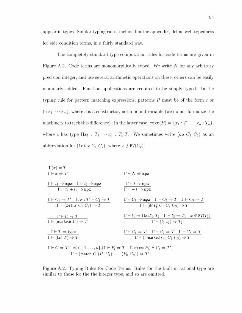
94
appear in types. Similar typing rules, included in the appendix, define well-typedness
for side condition terms, in a fairly standard way.
The completely standard type-computation rules for code terms are given in
Figure A.2. Code terms are monomorphically typed. We write N for any arbitrary
precision integer, and use several arithmetic operations on these; others can be easily
modularly added. Function applications are required to be simply typed. In the
typing rule for pattern matching expressions, patterns P must be of the form c or
(c x1 · · ·xm), where c is a constructor, not a bound variable (we do not formalize the
machinery to track this difference). In the latter case, ctxt(P ) = x1 : T1, . . . xn : Tn,
where c has type Πx1 : T1. · · ·xn : Tn.T . We sometimes write (do C1 C2) as an
abbreviation for (let x C1 C2), where x 6∈ FV(C2).
Γ(x) = T
Γ ` x⇒ T Γ ` N ⇒ mpz
Γ ` t1 ⇒ mpz Γ ` t2 ⇒ mpz
Γ ` t1 + t2 ⇒ mpz
Γ ` t⇒ mpz
Γ ` − t⇒ mpz
Γ ` C1 ⇒ T ′ Γ, x : T ′ ` C2 ⇒ T
Γ ` (let x C1 C2)⇒ T
Γ ` C1 ⇒ mpz Γ ` C2 ⇒ T Γ ` C3 ⇒ T
Γ ` (ifneg C1 C2 C3)⇒ T
Γ ` C ⇒ TΓ ` (markvar C)⇒ T
Γ ` t1 ⇒ Πx:T1. T2 Γ ` t2 ⇒ T1 x 6∈ FV(T2)
Γ ` (t1 t2)⇒ T2
Γ ` T ⇒ type
Γ ` (fail T )⇒ T
Γ ` C1 ⇒ T ′ Γ ` C2 ⇒ T Γ ` C3 ⇒ T
Γ ` (ifmarked C1 C2 C3)⇒ T
Γ ` C ⇒ T ∀i ∈ 1, . . . , n.(Γ ` Pi ⇒ T Γ, ctxt(Pi) ` Ci ⇒ T ′)
Γ ` (match C (P1 C1) · · · (Pn Cn))⇒ T ′
Figure A.2. Typing Rules for Code Terms. Rules for the built-in rational type aresimilar to those for the the integer type, and so are omitted.
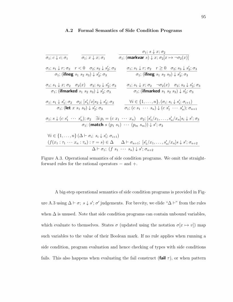
95
A.2 Formal Semantics of Side Condition Programs
σ1; c ↓ c; σ1 σ1; x ↓ x; σ1
σ1; s ↓ x; σ2σ1; (markvar s) ↓ x; σ2[x 7→ ¬σ2(x)]
σ1; s1 ↓ r; σ2 r < 0 σ2; s2 ↓ s′2; σ3σ1; (ifneg s1 s2 s3) ↓ s′2; σ3
σ1; s1 ↓ r; σ2 r ≥ 0 σ2; s3 ↓ s′3; σ3σ1; (ifneg s1 s2 s3) ↓ s′3; σ3
σ1; s1 ↓ x; σ2 σ2(x) σ2; s2 ↓ s′2; σ3σ1; (ifmarked s1 s2 s3) ↓ s′2; σ3
σ1; s1 ↓ x; σ2 ¬σ2(x) σ2; s3 ↓ s′3; σ3σ1; (ifmarked s1 s2 s3) ↓ s′3; σ3
σ1; s1 ↓ s′1; σ2 σ2; [s′1/x]s2 ↓ s′2; σ3σ1; (let x s1 s2) ↓ s′2; σ3
∀i ∈ 1, . . . , n, (σi; si ↓ s′i; σi+1)
σ1; (c s1 · · · sn) ↓ (c s′1 · · · s′n); σn+1
σ1; s ↓ (c s′1 · · · s′n); σ2 ∃i pi = (c x1 · · · xn) σ2; [s′1/x1, . . . , s′n/xn]si ↓ s′; σ3
σ1; (match s (p1 s1) · · · (pm sm)) ↓ s′; σ3
∀i ∈ 1, . . . , n (∆ ` σi; si ↓ s′i; σi+1)
(f(x1 : τ1 · · · xn : τn) : τ = s) ∈ ∆ ∆ ` σn+1; [s′1/x1, . . . , s′n/xn]s ↓ s′; σn+2
∆ ` σ1; (f s1 · · · sn) ↓ s′; σn+2
Figure A.3. Operational semantics of side condition programs. We omit the straight-forward rules for the rational operators − and +.
A big-step operational semantics of side condition programs is provided in Fig-
ure A.3 using ∆ ` σ; s ↓ s′; σ′ judgements. For brevity, we elide “∆ `” from the rules
when ∆ is unused. Note that side condition programs can contain unbound variables,
which evaluate to themselves. States σ (updated using the notation σ[x 7→ v]) map
such variables to the value of their Boolean mark. If no rule applies when running a
side condition, program evaluation and hence checking of types with side conditions
fails. This also happens when evaluating the fail construct (fail τ), or when pattern

96
matching fails. Currently, we do not enforce termination of side condition programs,
nor do we attempt to provide facilities to reason formally about the behavior of such
programs.
A.3 Helper Code for Resolution
The helper code called by the side condition program resolve of the encoded
resolution rule R is given in Figures A.4 and A.5. We can note the frequent uses
of match, for decomposing or testing the form of data. The program eqvar of Fig-
ure A.4 uses variable marking to test for equality of LF variables. The code assumes a
datatype of Booleans tt and ff. It marks the first variable, and then tests if the second
variable is marked. Assuming all variables are unmarked except during operations
such as this, the second variable will be marked iff it happens to be the first variable.
The mark is then cleared (recall that markvar toggles marks), and the appropriate
Boolean result returned. Marks are also used by dropdups to drop duplicate literals
from the resolvent.
A.4 Small Example Proof
Figure A.6 shows a small QF IDL proof. This proof derives a contradiction
from the assumed formula
(and (<= (- x y) (as_int (~ 1)))
(and (<= (- y z) (as_int (~ 2)))
(<= (- z x) (as_int (~ 3)))))
The proof begins by introducing the variables x, y, and z, and the assumption (named
f) of the formula above. Then it uses CNF conversion rules to put that formula into
CNF. CNF conversion starts with an application of the start rule, which turns the hy-
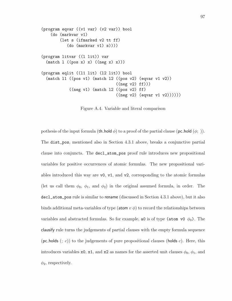
97
(program eqvar ((v1 var) (v2 var)) bool
(do (markvar v1)
(let s (ifmarked v2 tt ff)
(do (markvar v1) s))))
(program litvar ((l lit)) var
(match l ((pos x) x) ((neg x) x)))
(program eqlit ((l1 lit) (l2 lit)) bool
(match l1 ((pos v1) (match l2 ((pos v2) (eqvar v1 v2))
((neg v2) ff)))
((neg v1) (match l2 ((pos v2) ff)
((neg v2) (eqvar v1 v2))))))
Figure A.4. Variable and literal comparison
pothesis of the input formula (th hold φ) to a proof of the partial clause (pc hold (φ; )).
The dist_pos, mentioned also in Section 4.3.1 above, breaks a conjunctive partial
clause into conjuncts. The decl_atom_pos proof rule introduces new propositional
variables for positive occurrences of atomic formulas. The new propositional vari-
ables introduced this way are v0, v1, and v2, corresponding to the atomic formulas
(let us call them φ0, φ1, and φ2) in the original assumed formula, in order. The
decl_atom_pos rule is similar to rename (discussed in Section 4.3.1 above), but it also
binds additional meta-variables of type (atom v φ) to record the relationships between
variables and abstracted formulas. So for example, a0 is of type (atom v0 φ0). The
clausify rule turns the judgements of partial clauses with the empty formula sequence
(pc holds (; c)) to the judgements of pure propositional clauses (holds c). Here, this
introduces variables x0, x1, and x2 as names for the asserted unit clauses φ0, φ1, and
φ2, respectively.

98
(declare Ok type)
(declare ok Ok)
(program in ((l lit) (c clause)) Ok
(match c ((clc l’ c’) (match (eqlit l l’) (tt ok) (ff (in l c’))))
(cln (fail Ok))))
(program remove ((l lit) (c clause)) clause
(match c (cln cln)
((clc l’ c’)
(let u (remove l c’)
(match (eqlit l l’) (tt u) (ff (clc l’ u)))))))
(program append ((c1 clause) (c2 clause)) clause
(match c1 (cln c2) ((clc l c1’) (clc l (append c1’ c2)))))
(program dropdups ((c1 clause)) clause
(match c1 (cln cln)
((clc l c1’)
(let v (litvar l)
(ifmarked v
(dropdups c1’)
(do (markvar v)
(let r (clc l (dropdups c1’))
(do (markvar v) ; clear the mark
r))))))))
Figure A.5. Operations on clauses

99
(% x int (% y int (% z int
(% f (th_holds (and (<= (- x y) (as_int (~ 1)))
(and (<= (- y z) (as_int (~ 2)))
(<= (- z x) (as_int (~ 3))))))
(: (holds cln)
(start _ f
(\ f0
(dist_pos _ _ _ _ f0
(\ f1 (\ f2
(decl_atom_pos _ _ _ f1
(\ v0 (\ a0 (\ f3
(clausify _ f3
(\ x0
(dist_pos _ _ _ _ f2
(\ f4 (\ f5
(decl_atom_pos _ _ _ f4
(\ v1 (\ a1 (\ f6
(clausify _ f6
(\ x1
(decl_atom_pos _ _ _ f5
(\ v2 (\ a2 (\ f7
(clausify _ f7
(\ x2
(R _ _ _ x0
(R _ _ _ x1
(R _ _ _ x2
(assume_true _ _ _ a0 (\ h0
(assume_true _ _ _ a1 (\ h1
(assume_true _ _ _ a2 (\ h2
(idl_contra _ _
(idl_trans _ _ _ _ _ _ h0
(idl_trans _ _ _ _ _ _ h1
h2)))))))))
v2) v1) v0)
)))))))))))))))))))))))))))))))
Figure A.6. A small QF IDL proof

100
After CNF conversion is complete, the proof derives a contradiction from
those asserted unit clauses and a theory clause derived using assume_true (see Sec-
tion 4.3.2) from a theory contradiction. The theory contradiction is obtained with
idl_trans and idl_contra (Section 4.3.3).
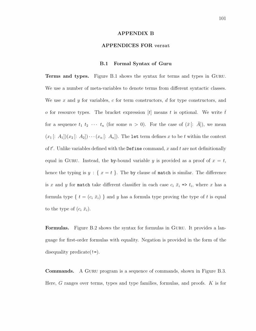
101
APPENDIX B
APPENDICES FOR versat
B.1 Formal Syntax of Guru
Terms and types. Figure B.1 shows the syntax for terms and types in Guru.
We use a number of meta-variables to denote terms from different syntactic classes.
We use x and y for variables, c for term constructors, d for type constructors, and
o for resource types. The bracket expression [t] means t is optional. We write t
for a sequence t1 t2 · · · tn (for some n > 0). For the case of (x [: A]), we mean
(x1 [: A1])(x2 [: A2]) · · · (xn [: An]). The let term defines x to be t within the context
of t′. Unlike variables defined with the Define command, x and t are not definitionally
equal in Guru. Instead, the by-bound variable y is provided as a proof of x = t,
hence the typing is y : x = t . The by clause of match is similar. The difference
is x and y for match take different classifier in each case ci xi => ti, where x has a
formula type t = (ci xi) and y has a formula type proving the type of t is equal
to the type of (ci xi).
Formulas. Figure B.2 shows the syntax for formulas in Guru. It provides a lan-
guage for first-order formulas with equality. Negation is provided in the form of the
disequality predicate(!=).
Commands. A Guru program is a sequence of commands, shown in Figure B.3.
Here, G ranges over terms, types and type families, formulas, and proofs. K is for
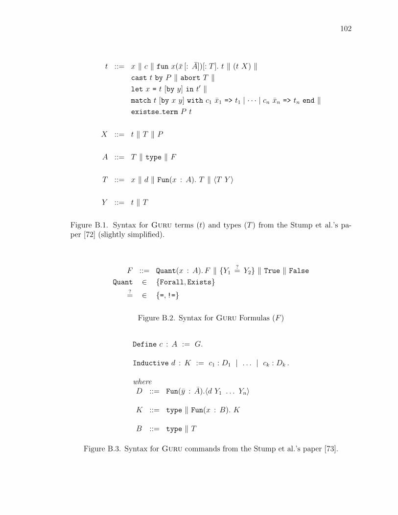
102
t ::= x ‖ c ‖ fun x(x [: A])[: T ]. t ‖ (t X) ‖cast t by P ‖ abort T ‖let x = t [by y] in t′ ‖match t [by x y] with c1 x1 => t1 | · · · | cn xn => tn end ‖existse term P t
X ::= t ‖ T ‖ P
A ::= T ‖ type ‖ F
T ::= x ‖ d ‖ Fun(x : A). T ‖ 〈T Y 〉
Y ::= t ‖ T
Figure B.1. Syntax for Guru terms (t) and types (T ) from the Stump et al.’s pa-per [72] (slightly simplified).
F ::= Quant(x : A). F ‖ Y1?= Y2 ‖ True ‖ False
Quant ∈ Forall, Exists?= ∈ =, !=
Figure B.2. Syntax for Guru Formulas (F )
Define c : A := G.
Inductive d : K := c1 : D1 | . . . | ck : Dk .
whereD ::= Fun(y : A).〈d Y1 . . . Yn〉
K ::= type ‖ Fun(x : B). K
B ::= type ‖ T
Figure B.3. Syntax for Guru commands from the Stump et al.’s paper [73].

103
kinds. Type and term constructors are introduced by the Inductive command, and
defined constants by the Define command.
B.2 Helper Code in the Guru Standard Library
Inductive bool : type :=
ff : bool
| tt : bool
Define primitive word := <vec bool wordlen>
Inductive list : Fun(A:type).type :=
nil : Fun(A:type). <list A>
| cons : Fun(A:type)(a:A)(l:<list A>). <list A>
Define eqlist :=
fun eqlist(A:type)(eqA:Fun(x y:A).bool)(l m:<list A>):bool.
match l with
nil _ =>
match m with
nil _ => tt
| cons _ _ m’ => ff
end
| cons _ a l’ =>
match m with
nil _ => ff
| cons _ b m’ => (and (eqA a b) (eqlist A eqA l’ m’))
end
end
Define member :=
fun member(A:type)(x:A)(l:<list A>)
(eqA:Fun(x1 x2:A).bool) : bool.
match l with
nil _ => ff
| cons _ h t => (or (eqA x h) (member A x t eqA))
end
Define list_all :=
fun list_all(A:type)(f:Fun(a:A).bool)(l:<list A>) : bool.
match l with
nil _ => tt
| cons _ a l’ => match (f a) with
ff => ff
| tt => (list_all A f l’)
end
end

104
Define list_subset :=
fun list_subset(A:type)(eqA:Fun(a b:A).bool)(l1 l2:<list A>) : bool.
(list_all A fun(a:A).(member A a l2 eqA) l1)
Define erase :=
fun erase(A:type)(eqA:Fun(x1 x2:A).bool)
(x:A)(l:<list A>) : <list A>.
match l with
nil _ => l
| cons _ y l’ =>
match (eqA x y) with
ff => (cons A y (erase A eqA x l’))
| tt => (erase A eqA x l’)
end
end

105
REFERENCES
[1] Agda: An interactive proof editor. http://agda.sf.net.
[2] The Coq proof assistant. http://coq.inria.fr.
[3] HOL4. http://hol.sourceforge.net.
[4] Isabelle. http://isabelle.in.tum.de.
[5] The SAT competitions. http://www.satcompetition.org.
[6] The SMT-EXEC service. http://www.smt-exec.org.
[7] The TraceCheck project. http://fmv.jku.at/tracecheck/.
[8] The Twelf project. http://twelf.plparty.org.
[9] Thorsten Altenkirch. Integrated verification in type theory. Lecture notes for acourse at ESSLLI 96, Prague, 1996. Available from the author’s website.
[10] Michael Armand, Germain Faure, Benjamin Gregoire, Chantal Keller, LaurentThery, and Benjamin Werner. A modular integration of SAT/SMT solvers toCoq through proof witnesses. In Jean-Pierre Jouannaud and Zhong Shao, edi-tors, Proceedings of International Conference on Certified Programs and Proofs(CPP), volume 7086 of Lecture Notes in Computer Science, pages 135–150.Springer, 2011.
[11] Henk Barendregt and Herman Geuvers. Proof-assistants using dependent typesystems. In Robinson and Voronkov [67], pages 1149–1238.
[12] HP Barendregt. Lambda calculi with types. Handbook of logic in computerscience, 2:117–309, 1992.
[13] Clark Barrett, Roberto Sebastiani, Sanjit A. Seshia, and Cesare Tinelli. Sat-isfiability modulo theories. In Armin Biere, Marijn Heule, Hans van Maaren,and Toby Walsh, editors, Handbook of Satisfiability, volume 185 of Frontiers inArtificial Intelligence and Applications, pages 825–885. IOS Press, 2009.
[14] Clark Barrett, Aaron Stump, and Cesare Tinelli. The SMT-LIB standard: Ver-sion 2.0. 2010.

106
[15] Clark Barrett and Cesare Tinelli. CVC3. In W. Damm and H. Hermanns, editors,Proceedings of the 19th International Conference on Computer Aided Verification(CAV’07), Berlin, Germany, volume 4590 of Lecture Notes in Computer Science,pages 298–302. Springer, 2007.
[16] Lujo Bauer, Scott Garriss, Jonathan M. McCune, Michael K. Reiter, JasonRouse, and Peter Rutenbar. Device-enabled authorization in the Grey system. InProceedings of the 8th Information Security Conference (ISC’05), pages 431–445,September 2005.
[17] Paul Beame, Henry A. Kautz, and Ashish Sabharwal. Towards understandingand harnessing the potential of clause learning. J. Artif. Intell. Res. (JAIR),22:319–351, 2004.
[18] Yves Bertot and Pierre Casteran. Interactive Theorem Proving and ProgramDevelopment. Coq’Art: The Calculus of Inductive Constructions. Texts in The-oretical Computer Science. Springer Verlag, 2004.
[19] Armin Biere. PicoSAT essentials. JSAT, 4(2-4):75–97, 2008.
[20] Sandrine Blazy, Zaynah Dargaye, and Xavier Leroy. Formal verification of a Ccompiler front-end. In FM 2006: Int. Symp. on Formal Methods, volume 4085of Lecture Notes in Computer Science, pages 460–475. Springer, 2006.
[21] Sascha Bohme and Tjark Weber. Fast LCF-style proof reconstruction for Z3.In Matt Kaufmann and Lawrence Paulson, editors, Interactive Theorem Prov-ing (ITP), volume 6172 of Lecture Notes in Computer Science, pages 179–194.Springer, 2010.
[22] Thomas Bouton, Diego Caminha B. de Oliveira, David Deharbe, and PascalFontaine. veriT: an open, trustable and efficient SMT-solver. In Renate A.Schmidt, editor, Proc. Conference on Automated Deduction (CADE), LectureNotes in Computer Science. Springer-Verlag, 2009. To appear.
[23] Robert Brummayer, Florian Lonsing, and Armin Biere. Automated testing anddebugging of SAT and QBF solvers. In Ofer Strichman and Stefan Szeider,editors, SAT, volume 6175 of Lecture Notes in Computer Science, pages 44–57.Springer, 2010.
[24] Ricky W. Butler and George B. Finelli. The infeasibility of experimental quan-tification of life-critical software reliability. In Proceedings of the conference onSoftware for citical systems, SIGSOFT ’91, pages 66–76, New York, NY, USA,1991. ACM.
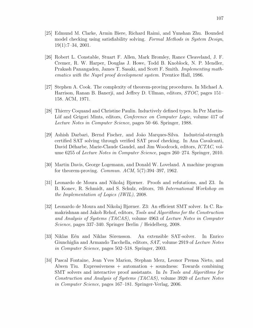
107
[25] Edmund M. Clarke, Armin Biere, Richard Raimi, and Yunshan Zhu. Boundedmodel checking using satisfiability solving. Formal Methods in System Design,19(1):7–34, 2001.
[26] Robert L. Constable, Stuart F. Allen, Mark Bromley, Rance Cleaveland, J. F.Cremer, R. W. Harper, Douglas J. Howe, Todd B. Knoblock, N. P. Mendler,Prakash Panangaden, James T. Sasaki, and Scott F. Smith. Implementing math-ematics with the Nuprl proof development system. Prentice Hall, 1986.
[27] Stephen A. Cook. The complexity of theorem-proving procedures. In Michael A.Harrison, Ranan B. Banerji, and Jeffrey D. Ullman, editors, STOC, pages 151–158. ACM, 1971.
[28] Thierry Coquand and Christine Paulin. Inductively defined types. In Per Martin-Lof and Grigori Mints, editors, Conference on Computer Logic, volume 417 ofLecture Notes in Computer Science, pages 50–66. Springer, 1988.
[29] Ashish Darbari, Bernd Fischer, and Joao Marques-Silva. Industrial-strengthcertified SAT solving through verified SAT proof checking. In Ana Cavalcanti,David Deharbe, Marie-Claude Gaudel, and Jim Woodcock, editors, ICTAC, vol-ume 6255 of Lecture Notes in Computer Science, pages 260–274. Springer, 2010.
[30] Martin Davis, George Logemann, and Donald W. Loveland. A machine programfor theorem-proving. Commun. ACM, 5(7):394–397, 1962.
[31] Leonardo de Moura and Nikolaj Bjørner. Proofs and refutations, and Z3. InB. Konev, R. Schmidt, and S. Schulz, editors, 7th International Workshop onthe Implementation of Logics (IWIL), 2008.
[32] Leonardo de Moura and Nikolaj Bjørner. Z3: An efficient SMT solver. In C. Ra-makrishnan and Jakob Rehof, editors, Tools and Algorithms for the Constructionand Analysis of Systems (TACAS), volume 4963 of Lecture Notes in ComputerScience, pages 337–340. Springer Berlin / Heidelberg, 2008.
[33] Niklas Een and Niklas Sorensson. An extensible SAT-solver. In EnricoGiunchiglia and Armando Tacchella, editors, SAT, volume 2919 of Lecture Notesin Computer Science, pages 502–518. Springer, 2003.
[34] Pascal Fontaine, Jean Yves Marion, Stephan Merz, Leonor Prensa Nieto, andAlwen Tiu. Expressiveness + automation + soundness: Towards combiningSMT solvers and interactive proof assistants. In In Tools and Algorithms forConstruction and Analysis of Systems (TACAS), volume 3920 of Lecture Notesin Computer Science, pages 167–181. Springer-Verlag, 2006.

108
[35] Harald Ganzinger, George Hagen, Robert Nieuwenhuis, Albert Oliveras, andCesare Tinelli. DPLL(T): Fast decision procedures. In R. Alur and D. Peled,editors, Proceedings of the 16th International Conference on Computer AidedVerification, CAV’04 (Boston, Massachusetts), volume 3114 of Lecture Notes inComputer Science, pages 175–188. Springer, 2004.
[36] Yeting Ge and Clark Barrett. Proof translation and SMT-LIB benchmark cer-tification: A preliminary report. In Proceedings of International Workshop onSatisfiability Modulo Theories (SMT), 2008.
[37] Allen Van Gelder. Independently checkable proofs from decision procedures:Issues and progress. In Geoff Sutcliffe and Andrei Voronkov, editors, LPAR,volume 3835 of Lecture Notes in Computer Science, page 1. Springer, 2005.
[38] Allen Van Gelder. Verifying rup proofs of propositional unsatisfiability. InISAIM, 2008.
[39] Herman Geuvers. Proof assistants: History, ideas and future. Sadhana, 34:3–25,2009. 10.1007/s12046-009-0001-5.
[40] Amit Goel, Sava Krstic, and Cesare Tinelli. Ground interpolation for combinedtheories. In R. Schmidt, editor, Proceedings of the 22nd International Conferenceon Automated Deduction (CADE), volume 5663 of Lecture Notes in ArtificialIntelligence, pages 183–198. Springer, 2009.
[41] Evguenii I. Goldberg and Yakov Novikov. Verification of proofs of unsatisfiabilityfor CNF formulas. In Design, Automation and Test in Europe Conference andExposition (DATE), pages 10886–10891. IEEE Computer Society, 2003.
[42] Carla P. Gomes, Bart Selman, and Henry A. Kautz. Boosting combinato-rial search through randomization. In Jack Mostow and Chuck Rich, editors,AAAI/IAAI, pages 431–437. AAAI Press / The MIT Press, 1998.
[43] Michael J. C. Gordon. From LCF to HOL: a short history. Proof, language, andinteraction: essays in honour of Robin Milner, pages 169–185, 2000.
[44] Michael J. C. Gordon, Robin Milner, and Christopher P. Wadsworth. EdinburghLCF, volume 78 of Lecture Notes in Computer Science. Springer, 1979.
[45] George Hagen and Cesare Tinelli. Scaling up the formal verification of Lustreprograms with SMT-based techniques. In A. Cimatti and R. Jones, editors,Proceedings of the 8th International Conference on Formal Methods in Computer-Aided Design (FMCAD), pages 109–117. IEEE, 2008.

109
[46] Robert Harper, Furio Honsell, and Gordon Plotkin. A framework for defininglogics. Journal of the Association for Computing Machinery, 40(1):143–184,1993.
[47] Gerwin Klein, Kevin Elphinstone, Gernot Heiser, June Andronick, David Cock,Philip Derrin, Dhammika Elkaduwe, Kai Engelhardt, Rafal Kolanski, MichaelNorrish, Thomas Sewell, Harvey Tuch, and Simon Winwood. seL4: Formalverification of an OS kernel. In J. Matthews and T. Anderson, editors, Proc.22nd ACM Symposium on Operating Systems Principles (SOSP), pages 207–220.ACM, 2009.
[48] Nupur Kothari, Todd Millstein, and Ramesh Govindan. Deriving state machinesfrom TinyOS programs using symbolic execution. In Proceedings of the 7th in-ternational conference on Information processing in sensor networks, IPSN ’08,pages 271–282, Washington, DC, USA, 2008. IEEE Computer Society.
[49] Daniel K. Lee, Karl Crary, and Robert Harper. Towards a mechanized metathe-ory of Standard ML. In Proceedings of 34th ACM Symposium on Principles ofProgramming Languages (POPL), pages 173–184. ACM Press, 2007.
[50] Xavier Leroy. Formal certification of a compiler back-end, or: programming acompiler with a proof assistant. In G. Morrisett and S. Peyton Jones, editors,33rd ACM symposium on Principles of Programming Languages, pages 42–54.ACM Press, 2006.
[51] Stephane Lescuyer and Sylvain Conchon. A reflexive formalization of a SATsolver in Coq. In Emerging Trends of the 21st International Conference onTheorem Proving in Higher Order Logics (TPHOLs), 2008.
[52] Bev Littlewood and Lorenzo Strigini. Validation of ultrahigh dependability forsoftware-based systems. Communications of the ACM, 36:69–80, 1993.
[53] Filip Maric. Formal verification of a modern SAT solver by shallow embeddinginto Isabelle/HOL. Theor. Comput. Sci., 411:4333–4356, November 2010.
[54] William McCune. Prover9 and Mace4. http://www.cs.unm.edu/~mccune/
prover9/, 2005–2010.
[55] Sean McLaughlin, Clark Barrett, and Yeting Ge. Cooperating theorem provers:A case study combining HOL-Light and CVC Lite. Electr. Notes Theor. Comput.Sci., 144(2):43–51, 2006.

110
[56] Steven P. Miller, Elise A. Anderson, Lucas G. Wagner, Michael W. Whalen, andMats P. E. Heimdahl. Formal verification of flight critical software. In AIAAGuidance, Navigation and Control Conference and Exhibit, AIAA-2005-6431,2005.
[57] Michal Moskal. Rocket-Fast Proof Checking for SMT Solvers. In C. R. Ramakr-ishnan and Jakob Rehof, editors, Tools and Algorithms for the Constructionand Analysis of Systems (TACAS), volume 4963 of Lecture Notes in ComputerScience, pages 486–500. Springer, 2008.
[58] Matthew W. Moskewicz, Conor F. Madigan, Ying Zhao, Lintao Zhang, andSharad Malik. Chaff: Engineering an efficient SAT solver. In DAC, pages 530–535. ACM, 2001.
[59] George Necula. Proof-carrying code. In 24th ACM SIGPLAN-SIGACT Sympo-sium on Principles of Programming Languages, pages 106–119, January 1997.
[60] Greg Nelson and Derek C. Oppen. Simplification by cooperating decision proce-dures. ACM Trans. Program. Lang. Syst., 1(2):245–257, 1979.
[61] Robert Nieuwenhuis, Albert Oliveras, and Cesare Tinelli. Abstract DPLL andabstract DPLL modulo theories. In F. Baader and A. Voronkov, editors, Proceed-ings of the 11th International Conference on Logic for Programming, ArtificialIntelligence and Reasoning (LPAR’04), Montevideo, Uruguay, volume 3452 ofLecture Notes in Computer Science, pages 36–50. Springer, 2005.
[62] Robert Nieuwenhuis, Albert Oliveras, and Cesare Tinelli. Solving SAT and SATmodulo theories: from an abstract Davis-Putnam-Logemann-Loveland procedureto DPLL(T). Journal of the ACM, 53(6):937–977, November 2006.
[63] Tobias Nipkow, Lawrence C. Paulson, and Markus Wenzel. Isabelle/HOL — AProof Assistant for Higher-Order Logic, volume 2283 of Lecture Notes in Com-puter Science. Springer, 2002.
[64] Duckki Oe, Andrew Reynolds, and Aaron Stump. Fast and flexible proof checkingfor SMT. In B. Dutertre and O. Strichman, editors, Workshop on SatisfiabilityModulo Theories (SMT), 2009.
[65] Duckki Oe, Aaron Stump, Corey Oliver, and Kevin Clancy. versat: A veri-fied modern SAT solver. In Viktor Kuncak and Andrey Rybalchenko, editors,VMCAI, volume 7148 of Lecture Notes in Computer Science, pages 363–378.Springer, 2012.

111
[66] Andrew Reynolds, Cesare Tinelli, and Liana Hadarean. Certified interpolantgeneration for EUF. In S. Lahiri and S. Seshia, editors, Proceedings of the 9thInternational Workshop on Satisfiability Modulo Theories (SMT), 2011.
[67] John Alan Robinson and Andrei Voronkov, editors. Handbook of AutomatedReasoning (in 2 volumes). Elsevier and MIT Press, 2001.
[68] Roberto Sebastiani. Lazy satisability modulo theories. Journal on Satisfiability,Boolean Modeling and Computation, 3(3-4):141–224, 2007.
[69] Natarajan Shankar and Marc Vaucher. The mechanical verification of a DPLL-based satisfiability solver. Electr. Notes Theor. Comput. Sci., 269:3–17, 2011.
[70] Joao P. Marques Silva and Karem A. Sakallah. GRASP - a new search algorithmfor satisfiability. In ICCAD, pages 220–227, 1996.
[71] Niklas Sorensson and Armin Biere. Minimizing learned clauses. In Oliver Kull-mann, editor, SAT, volume 5584 of Lecture Notes in Computer Science, pages237–243. Springer, 2009.
[72] Aaron Stump and Evan Austin. Resource typing in Guru. In J.-C. Filliatreand C. Flanagan, editors, Proceedings of the 4th ACM Workshop ProgrammingLanguages meets Program Verification, PLPV 2010, Madrid, Spain, January 19,2010, pages 27–38. ACM, 2010.
[73] Aaron Stump, Morgan Deters, Adam Petcher, Todd Schiller, and Timothy Simp-son. Verified programming in Guru. In Thorsten Altenkirch and Todd D.Millstein, editors, Programming Languges meets Program Verification (PLPV).ACM, 2009.
[74] Aaron Stump and Duckki Oe. Towards an SMT proof format. Proceedings ofthe Joint Workshops of the 6th International Workshop on Satisfiability ModuloTheories and 1st International Workshop on Bit-Precise Reasoning (SMT), pages27–32, 2008.
[75] Allen Van Gelder. Proof checker file format. http://users.soe.ucsc.edu/
~avg/ProofChecker/ProofChecker-fileformat.txt, 2004.
[76] Allen Van Gelder. Verifying propositional unsatisfiability: Pitfalls to avoid. InTenth International Conference on Theory and Applications of Satisfiability Test-ing, Lisboa, Portugal, 2007.

112
[77] Kevin Watkins, Iliano Cervesato, Frank Pfenning, and David Walker. A concur-rent logical framework I: Judgments and properties. Technical Report CMU-CS-02-101, Carnegie Mellon University, 2002.
[78] Tjark Weber. Integrating a SAT solver with an LCF-style theorem prover.PDPAR, Jan 2005.
[79] Tjark Weber. Using a SAT solver as a fast decision procedure for propositionallogic in an LCF-style theorem prover. Theorem Proving in Higher Order Logics(TPHOLs), 2005.
[80] Tjark Weber. Efficiently checking propositional resolution proofs in Is-abelle/HOL. In Chris Benzmuller, Bernd Fischer, and Geoff Sutcliffe, editors,Proceedings of the 6th International Workshop on the Implementation of Logics,volume 212 of CEUR Workshop Proceedings, pages 44–62, November 2006.
[81] Tjark Weber and Hasan Amjad. Efficiently checking propositional refutations inHOL theorem provers. Journal of Applied Logic, 7(1):26 – 40, 2009.
[82] Hantao Zhang. SATO: An efficient propositional prover. In William McCune,editor, CADE, volume 1249 of Lecture Notes in Computer Science, pages 272–275. Springer, 1997.
[83] Hantao Zhang and Mark E. Stickel. An efficient algorithm for unit propagation.In In Proceedings of the Fourth International Symposium on Artificial Intelli-gence and Mathematics (AI-MATH’96), Fort Lauderdale (Florida USA, pages166–169, 1996.
[84] Lintao Zhang and Sharad Malik. The quest for efficient boolean satisfiabilitysolvers. In Ed Brinksma and Kim Guldstrand Larsen, editors, CAV, volume2404 of Lecture Notes in Computer Science, pages 17–36. Springer, 2002.
[85] Lintao Zhang and Sharad Malik. Validating SAT solvers using an independentresolution-based checker: Practical implementations and other applications. InDesign, Automation and Test in Europe Conference and Exposition (DATE),pages 10880–10885. IEEE Computer Society, 2003.