on conjunctive normal form satisfiability
TRANSCRIPT

University of Pennsylvania University of Pennsylvania
ScholarlyCommons ScholarlyCommons
Technical Reports (CIS) Department of Computer & Information Science
November 1991
On Conjunctive Normal Form Satisfiability On Conjunctive Normal Form Satisfiability
Jon Freeman University of Pennsylvania
Follow this and additional works at: https://repository.upenn.edu/cis_reports
Recommended Citation Recommended Citation Jon Freeman, "On Conjunctive Normal Form Satisfiability", . November 1991.
University of Pennsylvania Department of Computer and Information Sciences Technical Report No. MS-CIS-91-94.
This paper is posted at ScholarlyCommons. https://repository.upenn.edu/cis_reports/339 For more information, please contact [email protected].

On Conjunctive Normal Form Satisfiability On Conjunctive Normal Form Satisfiability
Abstract Abstract This paper focuses on algorithms that solve CSAT (conjunctive normal form satisfiability) by searching for a satisfying truth assignment for the given formula F. We identify four basic ways to improve the basic search procedure: constraint propagators, simplifying transformations, heuristics, and other miscellaneous improvements. In each of these categories, we survey the existing improvements and suggest new ones. We lower the average time it takes to perform the simplest kind of constraint propagation from O(L) to O(L/P), where L is the length of F and P is the number of propositions in F; this
is optimal. We lower the current upper bound for CSAT from O(20.128 L) to O(20.128 (L-N)), where N is the number of clauses in F. Finally, we experimentally determine the fastest possible algorithm with respect to each of the basic improvements we consider.
Comments Comments University of Pennsylvania Department of Computer and Information Sciences Technical Report No. MS-CIS-91-94.
This technical report is available at ScholarlyCommons: https://repository.upenn.edu/cis_reports/339

On Conjunctive Normal Form Satisfiability
MS-CIS-91-94
Jon Freeman
Department of Computer and Information Science School of Engineering and Applied Science
University of Pennsylvania Philadelphia, PA 19104-6389
November 1991

On Conjunctive Normal Form Satisfiability
Jon Freeman Department of Computer and Information Science
University of Pennsylvania Philadelphia, PA 19104
November 1991
Abs t r ac t
This paper focuses on algorithms that solve CSAT (conjunctive normal form sa.tis- fiability) by searching for a satisfying truth assignment for the given formula F. We identify four basic ways to improve the basic sea,rch procedure: constraint propagators, simplifying transformations, heuristics, and ot,her miscella.neous improvements. In ea.ch of these categories, we survey the existing improvements and suggest new ones. We lower the average time it takes to perform the siniplest kind of constraint propagation from O(L) to o(+), where L is the length of F and P is the number of propositions in F; this is optimal. We lower the current upper bound for CSAT from 0(2°.128L) to 0 ( 2 ~ . l ~ " ' - ~ ) ) , where N is the number of clauses in F. Finally, we experimentally determine the fastest possible algorithm with respect to each of the basic improvements we consider.
1 Introduction
This paper focuses on algorithms that solve CSAT1 (conjunctive normal form satisfiability)
by searching for a satisfying truth assignlnent for the given formula F2. We identify four
basic ways to improve the basic search procedure: constraint propagators, simplifying trans-
formations, heuristics, and other nliscellaileous improvements. In each of these categories,
we survey the existing improvements and suggest new ones. We lower the average time it
takes to perform the simplest kind of constraint propaga,tion from O ( L ) to 0($) , where L
is the length of F and P is the number of propositions in F; this is optimal. (By average, we
mean averaged over any path through the search tree for F.) We lower the current upper
bound for CSAT from 0(2°.128L) to 0(2° .128(L-N)) , where h' is the number of clauses in F. 1 " CSAT" is not standard notation. My inspiration for t , l~is notation cornes from page 328 of Hopcroft
and Ullman [la]. We will focus exclusively on algorithms that yield exact solutions, ignoring the extensive body of research
on approxinlation algorithms for CSAT and other NP-hard problems.

Finally, we experimentally determine the fastest possible algorithm with respect to each of
the basic improvements we consider.
There are several reasons why I have chosen to study CSAT. First, CSAT is NP-
complete-in fact, it was the first problem proven to be NP-complete [4]. Second, CSAT
is the simplest kind of constraint satisfaction problem (CSP), and we can convert CSP's
to CSAT problems in polynomial time [40], so some of the complexity results for CSAT
are applicable to all CSP's. Third, relatively little research has been done on CSAT per
se; most researchers in this area have chosen to focus on CSP7s in general. Fourth, many
important problems reduce directly to CSAT, such as graph coloring, first-order theorem
proving, VLSI chip design, and some problems in computer vision [5, 13, 201. And fifth,
CSAT algorithms can take advantage of properties of Boolean algebra that the more general
CSP algorithms cannot3.
There is probably no one best CSAT algorithm, for two reasons. First, algorithms for
larger CNF formulas require more cleverness than algorithn~s for smaller ones do; in fact, for
reasonably sized CNF formulas, a brute-force a.pproac11 is usually best. Consequently, this
paper focuses on CSAT algorithms for larger CNF formulas. Second, some CNF formulas
are actually instances of CSP's that have been compiled down to the propositional calculus.
These expressions have special properties that we call take advantage of [40]; see Section
11.
2 Definition of CSAT
A proposition (or Boolea~z variable) is a variable that can he either true or false (denoted
by T and F, respectively). A literal l is either a proposition (say, p ) or the complement of
one (denoted by l p ) ; in the first case, we say that I is a positive literal, and in the second,
we say that 1 is a negative literal. We say that p is the proposition associated with l if either
1 =_ p or 1 G l p . A clause is a disjunction of literals associated with unique propositions. A
propositional formula is in conjunctive normal form (CNF) if it is a conjunction of unique
To be fair, I should add tha t CSP algorithms can t,ake a.dvant.a,ge of some results of graph theory that CSAT algorithms cannot.

clauses. For example,
is in CNF, where p, q, r , and s are propositions.
A truth assignment v is a partial function from the set of propositions to {T, F) . We
can extend the definition of v in a natural way so that i t assigns truth values to literals,
clauses and formulas. For a literal 1, if I p, then v(1) = v(p), otherwise v(1) = iv(p) . For
a clause C = Vy=l li, v(C) = VyZl v(li). For a formula F z Cj, v(F) = I\;=l v(Cj).
If * represents either a proposition, literal, clause, or formula, we say that v satisfies * if v(*) = T, and v falsifies * if ~ ( 4 ) = F. Note that v need not assign a truth value to every
proposition in F in order to satisfy (or falsify) F; this makes no difference in practice.
Since v is a partial function, we will say that formulas, clauses, literals, and propositions
can have one of three possible truth values with respect to v: T, F , or indeterminate
(denoted by I). Also, when we are discussing a truth a.ssignnient v in the contest of
a particular formula F , we will assume t11a.t the doma.in of v is restricted to the set of
propositions in F. Gallier provides a formal proof of the validity of this assumption [13].
The CNF-satisfiability problem (CSAT) is defined as follows [18]: Given a propositional
formula F in CNF, is there a truth assignment v that satisfies F?
3 Other Definitions and Notation
When trying to solve CSAT, we a1wa.y~ sta.rt with an empty trut.h a,ssignment. Let us call
this truth assignment v,.
We will frequently want to extend an esisting truth assignment by a proposition-truth
value pair. Given a truth assignment v, proposition 11, and truth value 7, we define v[r, t I]
as follows:
7 i f p = q 413 +- 4 ( q ) =
v(y) otherwise
Given a literal 1 and truth value T , we call also define v[l - I] in the obvious way:
v[p +- I] if 1 5 p for some p v[l + 71 =
v[p + 171 if 1 r l p for some p

Here are some parameters that we will use in our complexity analyses. Given a formula
F , L(F) is the length of F , i.e., the number of literals in F ; P ( F ) is the number of distinct
propositions in F ; and N ( F ) is the number of clauses in F. When F is understood from
context, we will refer to these parameters as L, P , and N respectively. We have the following
simple relationships among these parameters:
a L > 2N, because every clause should have length at least 2 (see Section 10.2), and at
least one clause should have length greater than 2-otherwise we could satisfy F in
polynomial time [ll].
L > 2P , because every proposition should occur at least twice in F, once as a positive
literal and once as a negative literal, otherwise we could simplify F immediately; see
Section 10.4.
a L 5 N P , because no clause can have more than P literals.
4 History and Related Work
The Davis-Putnam procedure is the first widely known CSAT algorithm [514. Other CSAT
algorithms include [37] and 1401.
Montanari defined constrai~lt satisfaction problenls [26]. Mackworth provides an excel-
lent overview of the field of constraint satisfaction [20]. There is a close relationship between
CSP's and truth maintenance systems: de Iileer explores this rela.tionship in detail [7], a8nd
Martins provides a bibliography of recent publica,tions that are relevant to both fields [22].
Bitner and Reingold were the first to articulate general principles of backtracking search
[2]. Stallman and Sussnian invented dependency-directed backtracking 1351. Gaschnig in-
vented another intelligent version of backtra.cking called ba.ckmarking [15]. Purdom et al.
invented multi-level dynamic search rearrangement 1321, which is a particular kind of con-
straint propagation algorithm [40].
A great deal of work has been done on the complexity of backtracking search. Due to the
nature of the topic, most of these studies have both theoretical and empirical components.
The Davis-Putnam procedure was actually invented about 50 years before Davis and Putnam, by L. Lowenheim [3].

Studies of a more theoretical nature include [17, 27, 31, 371; studies of a more empirical
nature include [9, 16, 31, 321; and studies in which both components are significant include
[15, 19, 301. The best known upper bound for CSAT is due to Allen van Gelder
[371
5 Solution Strategies
There are five main ways to solve CSAT (exactly) for a given CNF-formula F; only the last
three are widely used.
1. Enumerate all possible truth assignments and check ea,ch one to see whether i t satisfies
F.
2. Show directly that F is a colltradictioll by simplifying F completely and then checking
whether the resulting formula is equal to 1 (logical falsehood). If so, answer no, else
answer yes.
3. Show directly that F is unsatisfiable by using the resolution method.
4. With the aid of a theorem prover, show directly that the cornplemellt of F (a disjunc-
tive normal form expression) is valid. If so, answer no, else answer yes.
5. Show directly that F is satisfiable by searching through the space of possible truth
assignments for F.
The first approach takes time 0(2'); the second is not even known t o be in NP [13].
The resolution method is due to Robinson [33], and wa,s studied extensively by Galil [12].
Theorem proving is a rich field; Gallier gives references for theorem proving, and provides
a good introduction to both theorenl proving and resolution [13]. We will focus exclusively
on the last approach.

6 The Basic Algorithm
The basic algorithm is to do a depth-first search through the space of all possible truth
assignments until we either succeed or fail5.
Function Brute-Force(F, v) = case v(F) of
T => (true, v) I F => (false, v) ( I => let 1 = an indeterminate literal in the indeterminate clauses of F,
(bool, v') = Brute-Force(F, v[l c TI) in if boo1 then (true, v') else Brute-Force(F, v[E +- F]); end;
Initially, we call Brute-Force with F and v,.
Since CSAT is defined as a decision problem, we do not have to return the truth assign-
ment, but in practice, it would be silly not to do so.
7 Improvements to the Basic Algorithm
When we speak of improvements to CSAT, we must be careful. Some "improvements"
will unconditionally decrease the algorithm's running time, but others will decrease the
size of the search space at the expense of extra computation, and whether the decrease
in the one is worth the increase in the other is not immediately obvious6. Having said
this, there are four main ways to improve the basic algorithm: constraint propagators,
simplifying transformations, heuristics, and other miscellaneous improveme~lts Below, we
briefly describe these categories; we will discuss ea.ch one in ~nuch more detail in the sections
that follow.
a A constraint propagator is a function that takes a fornlula F and a truth assignment v
and returns a truth a.ssignment v' such that v C v' and we can satisfy F by extending v'
if and only if we can satisfy F by extending v. In other words, a constraint propagator
finds additional assignments of truth values to variables that necessarily follow from
I will write my pseudo-code in an ML-like functional style. I will occasionally use imperative c o ~ ~ s t r u c t s when they express more clearly the operation in question.
In Section 17, we will reach some conclusions about which improvernent.~ are genuine and which are not.

what we know about F and v. Constraint propagation is due to Montanari [26]. It
goes by many other names in the literature, including "discrete relaxation, domain
elimination, range restriction, filtering, and full-forward look-ahead algorithms" [20].
A simplifying transformation is just that: a function that takes a formula F and
returns a simpler formula F' such that F' ha.s a, ~a~tisfying truth assignment if and
only if F does. Most of these transformations are based on properties of Boolean
algebra, and thus are not applicable to CSP's in general.
In order to understand how simplifying transformations work, we must define the
notion of purging. Given a formula F and a truth assignllleilt v such that v(F) = I,
the purged version of F is the formula that contains the indeterminate clauses in F
and the indeterminate literals in those clauses. Let us call the function that returns
this formula Purge(F, v). It should be c1ea.r that we can sa.tisfy F by extending v if
and only if we can satisfy Purge(F, v) by estending v,. Purging can be either explicit
or implicit. Explicit purging involves repeatedly replacing (F, v) with (Purge(F, v), v,)
at every node in the search tree, and implicit purging does not-Purge(F, v) is always
implicit in F and v, hence the name.
There are two reasons why purging is of interest to us. First, we must purge an
indeterminate formula before applying a simplifying traasformation to i t , as these
transformations only affect a formula's indeterminate "core". Second, we can think
of explicit purging as a. simplifying tra.nsformation in its own right; if we shrink our
representation of F , subsequent operations on F will be that much faster. The biggest
problem with explicit purging is that it may yield duplica.te clauses, but duplicate
clauses do not affect the correctness of any of our sea.rch algorithms7, and they are
surely not worth the quadratic time it ta.kes to renlove them.
Explicit purging and other simplifying transformations are both used in [ 5 ] and [37],
although neither paper refers to them as such.
r A heuristic h is a function tha,t takes a formula F , a truth assignment v, and an
indeterminate literal 1 in F and returns a positive integer. This integer is an upper
They do, however, affect the correctness of one of our heuristics; see Section 11.

bound on the size of the subtree that would result from recursively calling the search
procedure with v[l t TI. If h somehow determines that extending v by (1,T) will
always lead t o an inconsistency, it returns a failure condition. (It need not make this
determination for all such literals, however.)
A heuristic gives us the ability to choose a good indeterminate literal to satisfy next
without having to actually explore the subtrees associated with these literals. Obvi-
ously, the running time of the heuristic should be substantially smaller than the time
it takes to explore these subtrees.
Heuristics are ubiquitous in search algorithms. Bitner and Reingold were probably
the first to describe heuristics for CSAT algorithms [2]. Zabih and McAllester describe
a heuristic that works well for CNF formulas containing a large proportion of binary
clauses [40] (see Section 11).
The miscellaneous improvements are hard to ca.tegorize, and are not worth listing
here; see Section 12.
8 Static Search versus Dynamic Search
Static search algorithms for CSAT are algorithms tl1a.t do not use heuristics to guide their
search. They may do some preprocessing on the formula. F before starting the search, and
they may use a constraint propa.gator during the search, but they sa,tisfy the literals in F
strictly from left to right. Dynamic search algorithms, on the other hand, do use heuristics
to guide their search; the order in which they satisfy the literals in F is hard to predict.
Below are two templates that show the general forill of static and dynamic search algo-
rithms, respectively. These templates show exactly where each kind of algorithm uses the
improvements described above.
Function Static-Template(F) = let F' = F with zero or more simplifying transformations applied to it in Static-Loop(Ft, v,) end;
Function Static-Loop(F, v) = let v' = v with a constraint propagator applied to it

in case vl(F) of T => (true, v')
1 F => (false, v') I I => let 1 = the leftmost indeterminate literal in the indeterminate clauses of F,
(bool, v") = Static-Loop(F, vl[l c TI) in if boo1 then (true, v") else Static-Loop(F, vl[l t F]) end
end;
In the following template, Apply-Heuristic(F, v, h) is a function that takes a formula
F , a truth assignment v, and a heuristic h and returns a indeterminate literal 1 in the
indeterminate clauses of F that, in terms of h, is the best one to satisfy next.
Function Dynamic- Template(F) = let Ff = F with zero or more simplifying transformations applied to it in Dynamic-Loop(F1, v,) end;
Function Dynamic-Loop(F, v) = let v' = v with a constraint propa.ga,tor a.pplied to it in case vl(F) of
T => (true, v') I F = > (false, v') I I => let Fr = Purge(F, v') with one or more simplifying transformations
applied to it (or just F for zero transformations), 1 = Apply-Heuristic(Ff, v', h) for some heuristic h, (bool, v") = Dynamic-Loop(Fr, vl[l +- TI)
in if boo1 then (true, v") else Dynamic-Loop(Fr, vr[l c F]) end
end;
9 Constraint Propagators
The basic idea behind a constraint propa,gator is simple. Suppose that we are trying to
satisfy a CNF formula F. If we know that satisfying a certain proposition p in F will yield
an inconsistency in every case, then p must be false; similarly, if we know that falsifying p
will yield an inconsistency in every case, then p must be true.
Constraint propagators vary in both their accuracy a,nd their running time, depending
on how far they look into the future. The simplest constraint propagator merely finds all
indeterminate propositions p in F such tha.t assigning some truth value to p imin,ediately

falsifies F. Following Zabih and McAllester, let us call this constraint propagator BCP, for
Boolean Constraint Propagation 1401. Here is the pseudo-code for BCP':
Function BCP(F, v) = let v' = BCP-Loop(F, v) in if v = v' then v else BCP(F, v') end;
Function BCP-Loop(F, v) = for all indeterminate propositions p in the indeterminate clauses of F do
if v[p t T](F) = F then v := v k t F] else if v[p t F](F) = F then v := v[p t TI;
return v;
Note that there are no constraints on the way in which we extend the original truth
assignment, i.e., the sequence of propositions we choose; 110 matter how we arrange the
propositions in this sequence, the final truth assignment is the same. McAllester provides
a formal proof of this assertion [23].
Below is a second version of BCP-Loop, and hence of BCP. The reader can verify that
these two algorithms are functionally equivalent, although they may appear to be different
at first.
Function BCP-Loop2(F, v) = for all indeterminate clauses C in F do
if C contains exactly one indeterminate literal 1 then v := v[E +- TI; return v;
A generalized version of the first algorithm for BCP is widely used in solving CSP's. To
wit, if a variable can have any of n possible values, where n > 2, and we know somehow
that n - 1 of those values will always lead to an inconsistency, then that variable must have
the nth value.
The running time of a constraint propagator clearly depends on the amount of lookahead
it does. Since BCP does the smallest amount of lookahead, we had better be able to
perform it quickly. David McAllester showed how to perform BCP in time O ( P ) [23]. This
seems optimal, since we can never extend a truth assignment more times than there are
propositions. It turns out, however, that the optimal running time of BCP is actually
I will explain later why I chose to write BCP-Loop as a separate function.

smaller, for consider the operation of BCP down any path of the search tree for F . The
length of any such path is O(P) . In the worst case, every clause in F will become eligible
for BCP, so we must keep track of each clause's eligibility status. In order to do this, we
must keep track of the truth value of each literal occurrence in F, which takes time R(L).
Therefore the optimal time bound for BCP is 0($) , averaged over any path through the
search tree for F. We present an algorithm that matches this bound in Section 14.1.2.
The next logical step up from BCP is the following constra.int propagator, called BCP2
Function BCP2(F, v) = let v' = BCP2-Loop(F, v) in if v = v' then v else BCP2(F, v') end;
Function BCP2-Loop(F, v) = for all indeterminate propositions p in the indeterminate clauses of F do
if BCP(F, v[p t T]) (F) = F then v := v[2~ c F] else if BCP(F, v[?, c F]) (F) = F then v := v[p c TI;
return v;
If we implement BCP2 exa.ctly as we have described it here, it will take far too ~nuch
time to be worthwhile. We can use special data structures, etc., to decrease BCP2's running
time, but even with these improvements in place, BCP2 still appears to be too slow to merit
serious consideration [40]. We will not discuss BCP2 any further.
Instead of having to settle for either BCP or BCP2, we ca.n compromise. Suppose we
have a fast constraint propagator Fast-BCP(F, v) that operates in much the same way that
BCP does, but takes less time a.nd is less powerful. Then we can define an intermediate
constraint propagator, called BCP-Plus, aa follows:
Function BCP-Plus(F, v, Fast-BCP) = let v' = BCP-Plus-Loop(F, v, Fast-BCP) in if v = v' then v else BCP-Plus(F, v', Fast-BCP) end;
Function BCP-Plus-Loop(F, v, Fast-BCP) = for all indeterminate propositions p in the indeterminate clauses of F do
if Fast-BCP(F, v[?, t T]) (F) = F then v := v[p t F] else if Fast-BCP(F, v[p t F]) (F) = F then v := v b + TI;
return v ;

Since Fast-BCP is an argument to BCP-Plus, the running time of BCP-Plus can fall
anywhere between the running times of BCP and BCP2.
We close this section by providing three examples of fast constraint propagators for
BCP-Plus.
1. BCP-Loop applied a constant number of times. (This is why I defined BCP-Loop
separately.)
2. BCP applied to the binary clauses in F , i.e., the clauses of length two. This constraint
propagator is not much faster than BCP when F contains lots of binary clauses, and
as I mentioned earlier, compiled CSAT forinulaa typically contain a large fraction of
binary clauses.
3. BCP applied to $ of the clauses in F, where n can vary. The clauses are chosen at
random from F.
10 Simplifying Transformat ions
The following subsections describe a total of seven simplifying transforma,tions. We ca.n
apply most of them dynamically, but the ma,in question is whether we should. As the
templates given above suggest, we can also apply them to F before we start the search, but
in practice, this usually does little or nothillg for us unless F is Inore or less random, i.e.,
i t is not a compiled version of a CSP.
10.1 Explicit Purging
As I mentioned earlier, we can think of explicit purging as a simplifying transformation in
its own right, as it shrinks the representation of F, and hence makes subsequent operations
on F that much faster. We will show how to perform explicit purging in linear time.
10.2 The Unit Clause Rules
A unit clause is a clause containing exactly one literal. The unit clause rules are from Davis
and Putnam [5] . They are the following identities of Boolean algebra:

where 1 is a literal and C' is a subclause.
If by applying the second rule, we manage to completely eliminate one or more of the
clauses in F , then F is a contradiction; for example, consider the formula ?i A 8 A ( a V b ) .
Note that the unit clause rules are the same as BCP, but with respect t o explicitly
purged formulas. If we intend to apply BCP to F at every node of the search tree, then
this transformation is clearly redundant.
10.3 Partial Simplificatioil
Partial simplification is an extension of the idea behind the unit clause rules: we apply a
set of Boolean identities to F. The identities we choose to apply naturally influence the
running time of this transformation. Experimentation has shown that the only identities
we can apply in a reasonable amount of time are the simplest ones, namely these:
~ A T ~ = I
F ' A L = L
l V 7 1 = T
C ' V T = T
F' A T = F'
1 A ( 1 V C') = 1 (the first unit clause rule)
1 A ( 1 1 V C') = 1 A C' (the second unit clause rule)
where 1 is a literal, C' is a subclause, and F' is a sub formula^.
Again, if we are running BCP at every node, we would not want to apply this transfor-
mation dynamically either.
10.4 The Positive and Negative Rules
These two rules first appeared in Davis and Putnam, where they were collectively referred
to as the affirmative-negative rule [5] . The idea is that if a proposition p in F occurs only
as a positive literal p, then we ca,il ma,ke p true and delete all clauses containing p f ro~n F.

Similarly, if p only occurs as a negative literal l p , then we can ma.ke p false and delete all
clauses containing - -~p from F .
We call apply this trailsforinatioll dynai~lically; consider the following formula:
Every proposition in this formula has both positive and negative occurrences, but if we
make b true, we can immediately make a true (since the last clause disappears).
10.5 Elementary Resolution
This transformation is from Davis and Putnam as well [ 5 ] . Let 11 be a proposition that
occurs exactly twice in F, once as a positive literal and once as a negative literal, i.e., we
can write F as
(PV C l ) A ( l P V C2)AF'
where C1 and C2 are subclauses, F' is a subformula, and C1, Cz, and F' are all free of p.
Then we can replace F by
(Cl V C2) A F'.
The idea behind this transformation is simple. We know that p must be either true
or false. If we make p true, then Purge(F, v) = C2 r\ F', and if we make p false, then
Purge(F, v) = C1 A F'. Taking the disjunction, we obtain the new version of F .
We may have to apply this transformation in stages, searching for eligible propositions
over and over. For example, consider the following formula:
We can only apply elementary resolution to b, but after we do so, we can then apply i t to
both c and d, etc.
In certain cases, we may be able to reduce F down to the null formula. If this happens,
we can conclude that F is satisfiable, although of course we cannot say exactly how.
We can apply this transformation dynamically: in the following formula, for example,

we cannot apply elementary resolution at all, but if we make a true, then we can apply it
to c (since the fourth clause is not present in Purge(F, u)).
10.6 Mixed ColIapsibility
Mixed collapsibility is due to Allen van Gelder [37]. The basic idea is this: Consider
two propositions p and q in F , and let 1, and 1, be literals (either positive or negative)
containing p and q respectively. If for every cla.use C in F, l p E C + lq E C , and l i p E C + 1 1 , E C , then we say that p collapses into q , and we delete all the clauses in F containing
p. Intuitively, we let the truth value of 1, equal the complement of the truth value of I ,
(whatever it may be), which immediately satisfies every clause containing p.
We can apply this transformation dynamically. Consider the following formula:
We cannot apply mixed collapsibility to this formula, but if we make c true, then a collapses
into b (since the last clause di~a~ppears).
10.7 Splitting Into Blocks
Suppose we can partition F into disjoint sets of clauses (or blocks) such that no two blocks
have any propositions in common. Then we can satisfy these blocks independently.
For every CNF formula F , we define an undirected graph G'(F) (or simply G) as followsg.
There are P vertices in G, each labeled with a proposition p in F. There is a path between
two vertices p and q in G if and only if two 1itera.l~ 1 , a.nd 1, both occur in at least one
clause in F , where E p and lq contain p and q, respectively. (We need only n - 1 edges for
each n-literal clause in order to ensure that this condition holds.) It should be clear that
the blocks of F correspond to the connected colnpollents of G. Furthermore, we call find
these connected compo~lellts by doing a depth-first search of G.
The running time of this transformation is the time it takes to construct G, find its
connected components, and break F into blocks. We ca.n construct G from a CNF-formula
F in time O(L1og P); in Section 14, however, we will describe a special data structure that
Our construction of G ( F ) launches us into the realm of CSP graphs. Dechter and Pearl have obtained several useful heuristics for CSP's by studying these kinds of graphs [9].
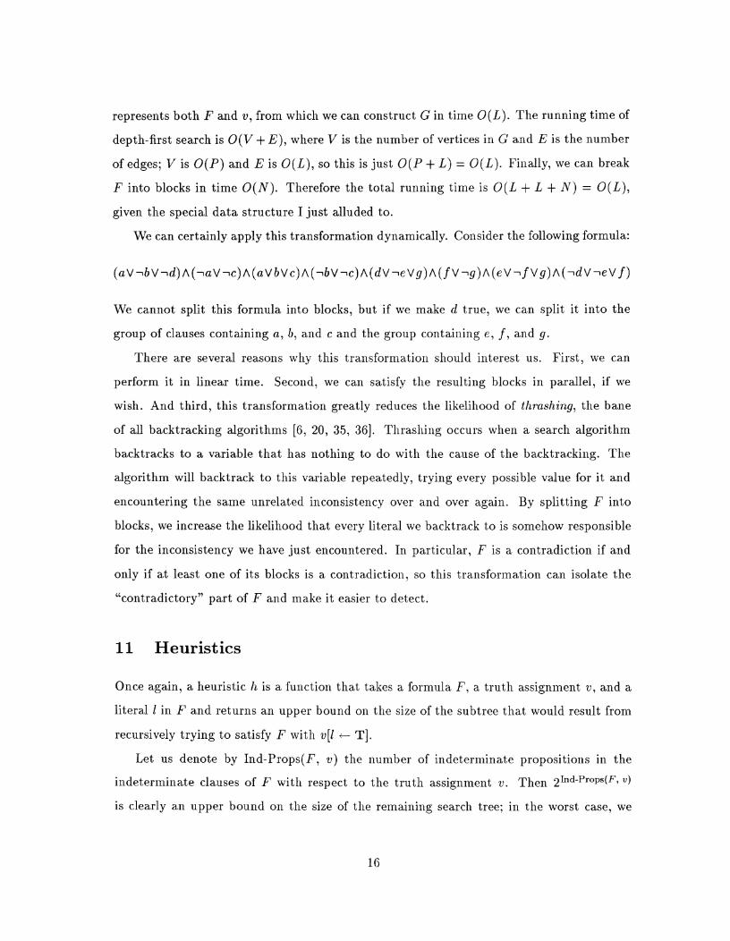
represents both F and v, from which we can construct G in time O(L). The running time of
depth-first search is O(V + E), where V is the number of vertices in G and E is the number
of edges; V is O ( P ) and E is O(L), so this is just O ( P + L) = O(L). Finally, we can break
F into blocks in time O(N). Therefore the total running time is O(L + L + N) = O(L),
given the special data structure I just alluded to.
We can certainly apply this transformation dynamically. Consider the following formula:
We cannot split this formula into blocks, but if we make d true, we call split it into the
group of clauses containing a , B , and c and the group containing e, f , and g.
There are several reasons why this transforlnation should interest us. First, we can
perform it in linear time. Second, we can satisfy the resulting blocks in parallel, if we
wish. And third, this transformation greatly reduces the likelihood of thrashing, the bane
of all backtracking algorithms [ G , 20, 35, 361. Thrashing occurs when a search algorithm
backtracks to a variable that has nothing to do with the cause of the backtracking. The
algorithm will backtrack to this variable repeatedly, trying every possible value for it and
encountering the same unrelated inconsistency over a,nd over again. By splitting F into
blocks, we increase the likelihood that every literal we backtrack to is somehow responsible
for the incolzsistency we have just encountered. In particular, F is a contradiction if and
only if a t least one of its blocks is a contra.diction, so this tra.nsforma.tion call isolate the
"contradictory" part of F and make it easier to detect.
11 Heuristics
Once again, a heuristic h is a function that takes a formula F, a truth assignment v , and a
literal 1 in F and returns an upper bound on the size of the subtree that would result from
recursively trying to satisfy F with v[l + TI.
Let us denote by Ind-Props($', v) the iluillber of indeterminate propositions in the
indeterminate clauses of F with respect to the truth assignment v. Then 2hd-P'0pS(Ft v,
is clearly an upper bound on the size of the reinaiili~lg search tree; in the worst case, we

might have to make every such proposition both true and false. Let us call this number
Basic-Estimate(F, v).
The number of heuristics one can think of is quite large: a heuristic can consist of a
constraint propagator and one or more simplifying transformations. However, a heuristic
must be both quick and accurate, otherwise a brute-force strategy will easily outperfornz i t
on reasonably sized problems. I have chosen three heuristics that I feel have a good chance
of meeting these criteria. Here they are, listed in decreasing order with respect to both
accuracy and computational overhead:
1. Let v' = BCP(F, v[l c TI). If v'(F) = T , return a cost of 0. If v t (F) = F, return a
failure condition. Otherwise, let F' = Purge(F, v'); break F' into blocks and return
the sum of the basic estimates for each block.
Note that calculating this heuristic involves doing a depth-first search for each literal
under consideration, a rather costly proposition [sic]. So why should we believe that
this heuristic night be useful? Because this heuristic finds the articulation points of
the graph G defined earlier-the literals in F that , when satisfied, break F up as
much as possible.
2. Let v' = BCP(F , v[l + TI). If vl(F) = T , return a cost of 0. If v t (F) = F, return a
failure condition. Otherwise, return Ba.sic-Estima.te(F, v'), i.e., do not brea,k F into
blocks.
3. A binary clause is a clause that contains exactly two literals. Let Open-Binaries(F, v,
1) be the number of binary clauses C in F such that both literals in C are indeterminate
and 1 C. ~~t~~~ 2 1 n d - P r ~ p ~ ( F , v)-Open-Binaries(F, v , - 1 ) .
This heuristic is due to Zabih and McAllester [40]. Intuitively, the idea is that when we
make l true, every binary cla,use co~ltailling 1 1 becomes eligible for BCP, decrementing
the number of propositions we might have to consider. We can think of this heuristic
as applying a special kind of fast constradnt propaga.tor to v, aa.mely one that takes
the literal 1 as an argument.
This heuristic works well when F conta,ins a la.rge proportion of bina.ry clauses, which

is usually the case when F is a compiled version of a CSP [40]. I t does not work
correctly when F contains duplicate clauses (as a result of explicit purging).
Zabih and McAllester developed this heuristic primarily because their own version of
BCP was too slow to be pa.rt of a practical heuristic [40]. Since our versio~l of BCP
runs in sublinear time on the average, it seems that it should be useful in a heuristic.
We will see, however, that this conjecture is not correct, either in theory or in practice.
We will analyze the running times of all three heuristics in Section 15 and compare them
experimentally in Section 17.
12 Misce1laneous Improvements
Now that we have examined the three illail1 kinds of improvements, we turn our attention
t o some other improvements that , while harder to categorize, can still decrease the search
time quite a bit.
1. Most CSAT algorithms jump from one indeterminate literal to the next, regardless
of where these literals occur [5, 32, 371. If we jump from one indeterminate cla~rse to
another, however, we are effectively looking farther into the search tree. In terms of
the search algorithm, this is wha,t we do: We extend the llotioll of the cost of a literal
with respect to a heuristic h to clauses by defiiling the cost of ail indeterminate clause
to be the sum of the costs of its indetermina.te literals. We select the clause having
the minimum total cost and try to satisfy it by repeatedly trying t o satisfy each of its
indeterminate literals until we ha.ve sa.tisfied a,t least one.
This improvement is due to Zabih and McAllester [40]. I t immediately lea,ds to three
others.
2. After we pick an indeterminate clause C to satisfy, we should not try t o satisfy its
indeterminate literals in any order; instea.d, we should try to satisfy them in increasing
order with respect to their estimated subtree size. Since we already know these sizes,
all we have to do to put this improvelnellt into pra.ctice is sort the indetermina.te
literals in the winning clause with respect to these sizes. This operation may appear

to increase Apply-Heuristic's running time, but we will show in Section 14.1.2 that it
does not increase its average running time down any path of the search tree.
To understand the next two improvements, note that our heuristics 1 and 2 can
occasionally detect when a literal 1 always leads to an inconsistency; heuristic 3 does
not have this property [40]. Let us call these literals failed literals, and all other literals
viable literals.
3. In procedure Apply-Heuristic, we should not consider the failed literals in F when
determining which indeterminate clause to satisfy next. More specifically, we sl~ould
base the cost of each illdeterlllillate clause on the costs of its viable literals, and after
we determine a winning clause, we should only sort and return the viable literals in
that clause.
4. If, in procedure Apply-Heuristic, we encounter at one or nlore indeterminate clauses
that contain nothing but failed literals, then we know that there is no way that we
can satisfy F, given the current truth assignment. In this ca.se, we should return an
empty list.
Given these improvements, our static and dynamic templates now look like this1':
Function Static-Template(F) = let F' = F with zero or more simplifying transfornlations applied to it in Static-Loopl(F1, v,, [ I) end;
Function Static-Loopl(F, v, lits) = if lits = [ ] then
let lits' = the indeterminate literals in the leftmost indeternlinate clause of F in Static-Loopl(F, v, Eits') end
else let (1::rest) = lits,
(bool, vl) = Static-Loop2(F, v[l t TI, [ 1 ) in if bool then (true, v') else Static-Loop2(F, v[l c F], rest) end;
Function Static-Loop2(F, v, lits) =
10 I t may be instructive to compare these templates to the templates in Section 8

let v' = v with a constraint propagator applied to it in case vl(F) of
T => (true, v') I F => (false, v') I I => let Eits' = the literals 1 in lits such that vl(l) = I
in Static-Loopl(F, v', lits') end
end;
Function Dynamic-Template(F) = let F' = F with zero or more simplifying tra.nsforma.tions a.pplied to it in Dynamic-Loopl(F1, v,, [ I ) end;
Function Dynamic-Loopl(F, v, lits) = if lits = [ ] then
let lits' = Apply-Heuristic(F, v, h) for some heuristic h in if lits' = [ ] then (false, v) else Dyna.mic-Loopl(F, v, lits') end
else let (1::rest) = lits,
(bool, v') = Dyna.mic-Loop2(F, v[1 +- TI, [ I ) in if boo1 then (true, v') else Dyizainic-Loop2(F, v[E t F], rest) end;
Function Dynamic-Loop2(F, v, lits) = let v' = v with a constraint propa.gator applied to it in case vl(F) of
T => (true, v') I F => (false, v') [ I => let F' = Purge(F, v') with one or more si~nplifying transformations
applied to it (or just F for no transformations), Zits' = the literals 1 ill lits such that v'(1) = I
in Dynamic-Loopl(F1, v', Zits') end
end;
13 An Ordering for Static Search
In the static search algorithms, we satisfy both t,he clauses in F and the literals within each
clause from left to right. We can try to minimize the search time by rearranging the clauses
and their literals before we start the search. Since we ca.nnot kilow in a,dvance which literals

we should satisfy first, all we have to rely on are general principles. In particular, we have
this principle: Try first where you are most likely to fail [2 , 161. In other words, the literals
that we should satisfy first are the ones that occur the most often in F. Hence we do the
following. First, we create a occurrence table for F : for each proposition p in F, we count
the nuniber of times p appears in F, either as a positive literal or as a negative literal. Next,
for each clause C in F, we find the sum of the number of occurrences associated with each
literal in C. Finally, we sort the clauses ill decreasilzy order with respect to these sums, and
within each clause we sort the literals in decreasing order with respect to their associated
number of occurrences.
Let us analyze the running time of this algorithm. We can construct the occurrence
table for F in time O ( L ) . We can find the occurrence count of each cla.use in time O ( L ) .
We can sort the clauses in time O(N log N). Finally, we can sort the literals within each
clause in time O(NP log P) . Hence we ca.n rearrange F to take advantage of the fail-first
principle in time O(L + L + N log N + NPlog P ) = O(NP1og P), which is not bad, since
we only have to reorder F once and we may derive substantial benefits from doing so. In
Section 17, we determine experimeatally how much of a difference this reordering makes.
In the next two sections, we examine the data structures and low-level procedures of
our CSAT algorithms in much greater detail.
14 Implementing the Basic Operations
This section describes our basic data structure and the basic operations that we perform
on it , and analyzes the running times of these operations. It has two parts. In the first
part, we consider data structures and ba.sic operations for clauses of constant length; in the
second part, we consider them for clauses of arbitrary length. I have split the section up in
this way for pedagogical reasons.
14.1 Implementation for Clauses of Col~stallt Leilgth
We begin by defining a data structure that represents the sta.te of a CSAT algorithm, i.e.,
one that contains information about both F and v.

14.1.1 Data Structures
Let us suppose that we have indexed the clauses in F, say in increasing order from left to
right. We define a five-component state vector as follows.
1. The first component is a t,riple <true-cs, false-cs, in.d-cs> called the F-triple, where
true-cs, false-cs, and ind-cs are integers which correspond to the nuiiiber of true, false,
and indeterminate clauses in F respectively.
2. The second component is an integer which corresponds to the nuiilber of indetermi-
nate propositions in F. Note that this is not necessarily the same as, and is in fact
greater than or equal to, the number of indeterminate propositions in the indeternzi-
nate clauses of F.
3. The third component is a. stack of integers called the BC'P-stack. The integers in this
stack are the indices of the clauses in F tliat are currently eligible for BCP, i.e., those
clauses tliat are indetermina.te and contain esactly one indeterminate literal.
4. The fourth component is a,n array of length N , called the N-array, which contains
information about the clauses in F. Ea.ch element of this array is a four-tuple <true-
Zits, false-lits, ind-lits, litprs>, where the first three coniponents are integers and the
fourth component is a list of (literal, integer) pairs. The first three numbers are the
number of true, false, and indeterniiaa.te literals in the cla,use in question, respectively;
litprs is a list of pairs of the form (I , P-index), where 1 is an indeterminate literal in
the clause and P-index is the index of l's proposition in the P-arruy, defined below.
5. The fifth component is an array of leilgth P, called the P-array, which contains
information about the propositions in F . The elements of this array are arranged in
increasing lexicographic order with respect to the propositions (since propositions are
just strings). Each elenleiit is a four-tuple <p, pos-lits, izeg-lits, I > , where p is a
string, pos-lits and neg-Zits are lists of integers, a.nd 7 is either T, F, or I. p is just
the proposition itself; pos-lits contains the indices of all the clauses in F in which the
literal p appears; neg-Zits contains the indices of all the cla.uses in which the literal l p
appears; and I is, of course, the current truth value of p.

The purpose of the state vector, of course, is to store information about F and v that is
correct at every step in the execution of the search algorithm. We maintain the correctness
of this information by updating the state vector every time we extend v (let us call the
function that does this Extend-Prop(u, p, I)). BCP takes advantage of the information in
the BCP-stack, and this is what makes it run faster. More specifically, whenever a clause in
F becomes eligible for BCP, Extend-Prop pushes its index onto the BCP-stack; BCP pops
these indices off the stack and processes each one by simply making an appropriate call to
Extend-Prop.
Let us determine how much time it takes to construct the initial state vector for F. It
takes time O(L log L) to find the set of propositions in F : we sort all of the propositions in F
into increasing lexicographic order in time O(L log L) and then remove adjacent duplicates
in linear time. Given this set, we can construct the P-array in time O(L1og P) : we do a
binary search of the P-array for every literal occurrence in F. Finally, we can construct the
N-array in time O(N) and the remaining three componel~ts in constant time, for a bound
of O(LlogL+ L l o g P + N ) = O(L1ogL).
14.1.2 Algorithms and Running Times
Next, we show how to use this data structure to perforin the basic operations of our CSAT
algorithms and analyze the running time of each operation. We describe simple operations
before complicated ones.
To calculate the truth value of any proposition p in F, given a pair (p, P-index), we
simply find the P-indexth element of the P-array and return its fourth component.
This takes constant time.
To calculate the truth value of any literal 1 in F, given a pair ( I , P-index): If E = p
for some proposition p, we return the truth value of p; if I r l p for some p, we return
the complement of the truth value of p. This takes constant time as well.
To calculate the truth value of any clause C in F, given its index C-index, we examine
the C-iizdexth element of the N-array. If true-lits > 0, then C is true; if true-lits =
2nd-lits = 0, then C is fa,lse; otherwise, C is indetermina.te. This ta,kes consta.nt time.

To calculate the truth value of F itself, we just examine the F-triple. If false-cs > 0,
then F is false; if false-cs = ind-cs = 0, then F is true; otherwise, F is indeterminate.
This takes constant time as well.
To calculate the number of indeterminate propositioils in F , we simply return the
second component of the state vector in constant time. Note that this number is not
necessarily equal to, and may in fact be greater than, Ind-Props(F, v)-the number
of indeterminate propositions in the indeternzinate cluuses of F. Ind-Props(F, v)
provides a better estimate of the remaining search tree size; using our state vector,
however, it would take time O(L) to calculate. Given this tradeoff, returning the sec-
ond component is probably the wiser choice. The main consequence of this difference
is that my implementatioils of the three heuristics in Section 11 do not correspond
exactly t o the way I defined them.
Procedure Apply-Heuristic needs to have the set of indeterminate literals in the inde-
terminate clauses in F, written as a list of (1, P-index) pairs. Do construct this list,
we run through the P-army. For each tuple of the form <p, poslits, neglits, I>, we
check if I = I. If so, and a t least one of the clauses in poslits is indeterminate, we
add (p, P-index) to the list, where P-index is the index of the tuple in question; if a t
least one of the clauses in neglits is indeterminate, we add (-111, P-index). This takes
time O(L).
To recover the current truth a.ssignn1ent from the sta,te vector as a list of proposition-
truth value pairs, we run through the P-array, collecting such a pair for all propositioils
that are not indeterminate. This takes time O(P) .
Next, we turn our attention to the three basic operations that concern us most: Extend-
Prop, B CP, and Apply-Heuristic.
To perforni Extend-Prop:
Let us assume t1la.t we a.re making a. proposition p true. (The case where we a,re
making p false is similar.) We are given the pair (p, P-index). First, we decrement the
second component of the state vector, i.e., the number of indeterminate propositions

in F. Then we find the P-indexth element of the P-array (in constant time), i.e.,
<p, pos-lits, neg-Zits, I> (actually, we know that 7 must be I). We set 7 to T.
Next, for each C-index in pos-Eits, we find the C-indexth element of the N-array (in
constant time), i.e., <true-Eits, false-lits, ind-Zits, lit-list>. We modify this tuple by
incrementing true-lits, decrementing ind-lits, and deleting (p, P-index) from lit-list,
all in constant time1'. If, as a result of these operations, we have satisfied this clause
for the first time, we modify the F-triple <true-cs, false-cs, ind-cs> by iilcrementing
true-cs and decrementing iizd-cs, also in constant time. Finally, for each C-index iin
neg-lits, we find the C-indexth element of the N-array (in constailt time). We modify
this tuple to record the effects of making the literal l p false. If by doing so, we have
falsified this clause, we modify the F-triple accordingly; or, if we have made this clause
eligible for B C P ' ~ (i.e., true-lits is 0 and ind-lits ha,s become I), we push the index of
this clause onto the BCP stack (in constant time).
Notice that Extend-Prop pushes indices onto the BCP-stack, but it never pops them
off of it. This is the respollsibility of BCP it,self (described below).
Now, consider the operation of Extend-Prop dowil one path of the search tree for F.
Extend-Prop takes coizstant time to process ea.ch index in both pos-lits and neg-lits.
All of the calls to Extend-Prop will process a total of O(L) such indices, for an average
time bound of o($).
To extend the truth assignment v by a literal-truth value pair (1, I), we determine
whether 1 is a positive or a negative literal. If 1 = p for some p, we extend v by (p, 7 ) ;
if 1 = l p for some p, we extend v by (p, 1 7 ) . This takes average tiine o($) as well.
To perform BCP:
First, we pop a clause index off of the BCP-stack. Then we use this index to find the
N-array tuple associated with this clause (in const ant time), i.e., < true-lits, false-lits,
ind-lits, litprs>. We double-check that this clause is in fa,ct still eligible for BCP; if 11 We can delete p from lit-list in constant time because, again, we are assuming that every clause has
constant length. l 2 There is some equivocation in this discussion between the algorithm for BCP and the procedure that
performs i t .

not, we go on to the next index in the stack. (Under certain circumstances, it may
be possible for a clause to lose its eligibility for BCP while its index is on the BCP-
stack.) Now there is exactly one pair ( I , P-index) in litprs; we call Extend-Prop in the
appropriate way to satisfy this literal, and repeat until the BCP-stack is empty. (The
point, of course, is that Extend-Prop may add still more indices to the BCP-stack, so
the length of the stack need not strictly decrea.se as we execute BCP.)
Let us analyze the running time of BCP down one path of the search tree for F. The
time it takes for BCP to process each index on the BCP-stack is at most the running
time of Extend-Prop, or o($) on the average. The total number of indices that
Extend-Prop will push onto the BCP-stack is O(N) (at most one index per clause),
but BCP will discard some of these indices, as noted above; in fact, the total number
of indices for which BCP will call Extend-Prop is O(P) . Hence the average running
time of BCP is just 0($$) = 0($).
a To perform Apply-Heuristic:
Say that the heuristic in question (call it h) runs in time H. First, we find the set of
all indeterminate literals in the illdeterminate clauses in F (described above). Next,
we apply h to each of these literals, creating a ta.ble of literal-cost pairs. For each
indeterminate clause in F, we find the sum of the costs of all of its indeterminate liter-
als. Finally, we find the clause having the minimum total cost, sort its indeterminate
literals by increasing cost, and return this sorted list.
Let us analyze the running time of this procedure. We can find the set of indeterininate
literals in F in time O(P) . l i e can build the cost table in time O(PH)13 . Using some
additional data structures, we can propa.ga.te the information in this table to all of the
clauses in F in time O(L). We can find the cla>us-e with the minimum total cost in time
O(N). And finally, we can sort the literals in the winning clause in time O(P1og P ) .
Note, however, that on any one path through the search tree for F, Apply-Heuristic 13 This is actually a bit tricky. My heuristics take a s tate vector as an argument, and some of them
modify this s ta te vector (by performing BCP 011 it). This seems to indicate that we have to pass a fresh copy of the s tate vector t o the same heuristic for every literal under consideration, which would take time R ( P 2 ) . I got around this problem by recording the changes that a heuristic makes to the s ta te vector for a given literal, and then undoing those changes before proceeding with the next literal. Section 17 discusses a similar modification t o the top-level algorithms.

will return at most P literals, so it will never have to sort more than P literals at once,
for a total time bound of O(P1og P), or O(1og P ) on the average. Hence the average
running time of Apply-Heuristic is O ( P + P H + L $ log P) = O(max(L, PH) ) .
14.2 Implementation for Clauses of Arbitrary Length
In this subsection, we relax our assumption that every clause in F has constant length. In
the general case, a clause can have length at most P, because it cannot have more literals
than there are propositions. We show how, by slightly com~>licating the state vector of the
previous section, we can still perform BCP and Extend-Prop in average time o($).
14.2.1 Data Structures
Like the original state vector, our new state vector has five components: an F-triple, an
indeterminate proposition counter, a BCP-sta,ck, a,n N-a.rray, a.nd a P-a.rray. Only the last
two components (the N-array and the P-array) are different.
Each element of the N-array is a 5-tuple < true-lits, false-Zits, ind-Zits, Lit-array, Lit-
array-ptr>, where true-lits, false-lits, and ind-lits are exa.ctly as before, Lit-array is
an array whose length is the lellgth of the clause in question, and Lit-array-ptr is an
integer. For a clause C, the it11 element of Lit-array is a triple (1 , P-index, Jag), where
1 is a literal in C, P-index is an integer, and f lag is a, boolean. 1 is just the ith literal in
C, P-index is as before, a,nd Jug indica.tes whether v(l) # I. Lit-army-ptr is the index
of a triple in Lit-array such that the literal in this triple is the leftmost indeterminate
literal in Lit-array.
a Each element of the P-array is a 4-tuple <p, pos-Zits, neg-lits, I>, a.s before. The
contents of pos-Zits and neg-lits are different, however: instead of just containing clause
indices, they contain pairs of integers of the form (C-index, 1-index). As before, C-
index is the index of a clause C containing the a.ppropriate literal; 1-index is this
literal's index in C's Lit-army.
What we are essentially doing is indexing the literals in every clause (say in increasing
order from left to right), and replacing litprs in the N-a,rra,y's tuples with a.rrays that contain
information about every literal in their associated clauses.
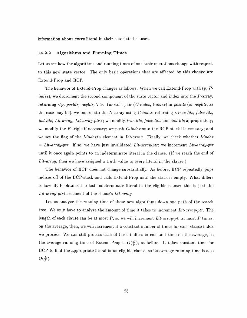
14.2.2 Algorithms and Running Times
Let us see how the algorithms and running times of our basic operations change with respect
t o this new state vector. The only basic opera.tions tha.t are affected by this change are
Extend-Prop and BCP.
The behavior of Extend-Prop changes as follows. When we ca.11 Extend-Prop with (11, P-
index), we decrement the second component of the state vector and index into the P-array,
returning <p, poslits, neglits, 7>. For each pair (C-index, 1-index) in yoslits (or neglits, as
the case may be), we index into the N-array using C-index, returning <true-lits, false-lits,
ind-lits, Lit-array, Lit-array-ptr>; we modify true-Zits, false-kits, and ind-lits appropriately;
we modify the F-triple if necessary; we push C-index onto the BCP-sta,ck if necessary; and
we set the flag of the I-iizdexth elenlent in Lit-array. Finally, we check whether I-index
= Lit-array-ptr. If so, we have just invalida,ted Lit-array-ptr; we increment Lit-arruy-ptr
until it once again points to an indeterminate literal in the clause. (If we reach the end of
Lit-array, then we have assigned a truth value to every literal in the clause.)
The behavior of BCP does not change substantially. As before, BCP repeatedly pops
indices off of the BCP-stack and calls Extend-Prop until the stack is empty. What differs
is how BCP obtains the last indeterminate literal in the eligible clause: this is just the
Lit-array-ptrth element of the cla.use's Lit-array.
Let us analyze the running time of these new algorithms down one path of the search
tree. We only have t o analyze the amount of time i t talies to illcrelneilt Lit-array-ptr. The
length of each clause can be at most P , so we will increlnent Lit-array-ptr a t most P times;
on the average, then, we will increment i t a constant number of times for each clause index
we process. We can still process ea.ch of these indices in consta.nt time on the average, so
the average running time of Extend-Prop is O ( j ) , as before. It takes coilstant time for
BCP to find the appropriate literal in an eligible clause, so its average running time is also
O(+).

15 Implementing the Heuristics
To complete our discussion of our implementations, we need only analyze the running tiines
of our three heuristics. To do this, we first need to say something a.bout the running time
of BCP, as Heuristics 1 and 2 both use it.
We have shown that our implementation of BCP takes time o($) on the average with
respect t o any path through the search tree for F. We have not shown, however, that all of
the O ( P ) possible calls t o BCP at any particular node (one for each indeterminate literal)
take 0 ( $ ) time on the average, i.e., O ( P ) time total; this is simply not true in general. All
we can say about these calls to BCP is that they take O ( P ) time each, and hence O ( P 2 )
time total, a disappoillting result. Therefore the running time of Heuristic 1 is O(L + P) =
O(L) and the running time of Heuristic 2 is O ( P ) .
To implement Heuristic 3, we only have to implement the function Open-Binaries. (Re-
call that Open-Binaries(F, v, 1 ) is the number of binary clauses C in F such that both
literals in C are indeterminate and 1 E C.) Given a pair (1, P-index), we index into the
P-array, returning the tuple <p, po.slits, neglits, T>. Then we simply count the number of
open binary clauses whose indices are in either poslits or neglits. This takes time o($) on
the average, or total time O(L) .
Even though Heuristic 3 is theoretically faster than Heuristics 1 and 2, one of the latter
heuristics may still outperforln it in practice. We deternliile whether this is the case in
Section 17.
16 Lowering the Upper Bound for CSAT
The best known upper bound for CSAT is currently 0(2°.12SL), due to Allen van Gelder
[37]. If our search algorithm uses BCP, we know that we only have to explicitly change the
truth value of n - 1 of the literals in any cla.use of length n. This immediately drops van
Gelder's upper bound to 0 ( 2 ~ . ' * ~ ( ~ - ~ ) ) , since his algorithm does not use BCP. To show
that this is a genuine reduction in the upper bound, it suffices to show that N cannot be a
constant; that is, if N is a consta.nt, then we call satisfy F in polynomial time.
Theorem: We can satisfy a,ny CNF formula. F in time ( 2 ~ ) ~ "

Proof: By inductioil on N
Base case ( N = 1): To satisfy one clause, we simply satisfy any of the literals in that clause.
Inductive hypothesis (N = k): Suppose that we ca.n satisfy F in time ( 2 ~ ) ~ .
Inductive step ( N = k + 1): We can satisfy F using the following algorithm.
For each proposition p in F:
1. Make p true. If any clauses in F are false, return no. Otherwise, a t least one clause in
F is now true, so at most k clauses in F are now indeterminate14. Recursively try to
satisfy the indetermimte cla.uses. By the inductive hypothesis, this ta.kes time ( 2 ~ ) ~ .
2. If we fouild a way to satisfy F in step 1, return yes. Otherwise, we do the same thi~lg
with p set to false.
This algorithm will certainly find a satisfying truth a.ssignment for F if one exists, and
it runs in time 2 P x ( 2 ~ ) ~ = ( 2 ~ ) ~ + l .
The next sectioil describes the results of experiments I undertook to determine which
of the most promising improvements listed a.bove is in fa,ct the fastest.
17 Experimental Results
The main question we would like to answer is this: How inucll time should we spend doing
clever things at each node of the search tree? If we spend too much time, the average search
tree size will be small but the overhead will negate our efforts. 011 the other hand, if we
do not spend enough time at each node, the algorithm will make too many bad decisions.
No matter what we do, of course, the runniilg time will still increase exponeiltially with
the problem size; our objective is to maximize the problem size at which this becomes
inconvenient.
I implemented a total of five different CSAT algorithms, two static and three dynainic.
All of the algorithms performed BCP at every node. One static algorithm did reordering
l4 I am assuming tha t we have applied t,he positive and negat,ive rules to F. Doing so guarantees that for every proposition p in F, the literals p and - p each occur a t least once, so extending the t ru th assignment in any way whatsoever will always satisfy a t least one clause.

before starting the search and t.he other did not. The dyna,mic algorithms differed in terms
of which simplifying transformations they performed, if any: the first dynamic algorithm
performed no simplifying transformations whatsoever; the second performed explicit purg-
ing at every node; and the third performed both explicit purging (necessarily) and splitting
into blocks at every node. For each dynamic search algorithm, I tried the three heuristics
described in Section 1115.
Note that I only iinplemented two of the seven simplifying transforlnations listed in
Section 10. I did this because these two transformations appear t o be the best of the seven;
they run in linear time and they are appealing for other reasons, as discussed earlier. At
any rate, it turns out that even these transforlnations did not perform well enough to be
useful (see below), so it is highly unlikely that the other five would improve things either.
The goals of my experiments were these:
To compare the three heuristics listed in Section 1ll6.
To compare static search with and without the ordering described in Section 13.
To determine the feasibility of splitting F into blocks in either the main algorithm, a
heuristic, or both.
To compare the best of the dyna.mic sea.rch algorithms t,o the best of the static search
algorithms.
I wrote these algorithms in Standard ML of New Jersey17. All three algorithms shared
the same data structures and low-level code, and all three were written in exactly the same
way to lend some legitimacy to the comparisons.
One technical point I should make about my inlplementation is that my top-level ML
functions do not resemble the top-level pseudo-functions t11a.t appear elsewhere in this paper.
The functions in this paper are recursive, a.nd hopefully elegant, but require that we make
a copy of the state vector at every node of the search tree. Since the size of the state vector
l5 I could not, however, try Heuristic 3 with the second and third dynamic search algorithms because of their use of explicit purging.
16 Again, my implementation of these heuristics differs slightly from the way I described them. l7 T h e source code is freely available to anyone who wishes to verify these results.

is linear in F, this automatica.lly adds an enormous amount of overhead to the algorithms.
My ML functions use explicit backtracking and rely on a stack which contains the changes
made to the state vector while progressing down the current branch of the search tree.
Clearly, the larger the state vector, the more important it is to iinplelnent the algorithms
in this way.
I measured the performance of each algorithm in three u7a.ys: the number of times it
extends the truth assignment for F, the size of the search tree it generates for F, and the
amount of time it takes to satisfy F (the most iniportant criterion). The formulas I used
were randomly generated, and corresponded to graph coloring problems. More specifically,
the pair ( N , p ) represents a family of gra.ph-coloring problems, where N is the number of
nodes in the graph and p is the probability of a.n edge occurring between any pair of nodes.
I tried to choose (N, p) pairs for which an avera.ge problelrl instance is just as likely to have
no solutions as it is to have at least one solution. I cannot say anything, however, about
the exact frequency with which these alternatives occur.
The following table lists the avenge CPU time in seconds Is for several interesting
problem instance-search algorithm combinations. I obtained these results on a Sun 4/490
running version 0.66 of Standard ML of New Jersey. The (N,p) pairs represent problem
instances, as described above. The abbreviations denote search algorithms as follows:
S-Plain Static search with BCP and no reordering.
S-Reorder Static search with BCP and reordering.
D-Plain-H1 Dynamic seasch with BCP, no simplifying transforma.tions, a,nd Heuristic 1.
D-Plain-H2 Same as above. but with Heuristic 2.
D-Plain-H3 Same as above, but with Heurisbic 3.
D-Purge-H1 Dynamic search with BCP, explicit purging, and Heuristic 1.
D-Purge-H2 Same as above, but with Heuristic 2.
18 Not including garbage collection time.

D-Split-H1 Dynamic search with BCP, (explicit purging,) splitting into blocks, and Heur-
istic 1.
D-Split-H2 Same as above, but with Heuristic 2.
Blank entries in the table denote combinations with running times that are too long t o care
about (or t o measure easily).
Given the data in this table, we ca.n reach the following conclusions:
Static search with reordering is better than sta.tic search without i t , although both
algorithms get out of hand quickly.
In general, dynamic search is better than static sea,rch.
Out of the three heuristics under consideration, Heuristic 3 is the best. Heuristic 1 is
hardly worth considering.
a With respect to the simplifying transformations, not perforining any transformations
a t all is the best strategy.
The fastest algorithin overall is D-Plain-3: dynamic sea.rch with BCP, no simplifying
transformations, and Heuristic 3.

This data indicates that tlrere seems to be little room for error wit11 respect to CSAT
algorithms. On the one hand, we see that a small amount of cleveriless is absolutely essential
if we are to have even reasonably useful CSAT algorithms, i.e., our search algorithms must
be dynamic. On the other hand, the amount of work we should do a t each node in the
search tree should be very small. The extreme nature of these results may be partially due
to the fact that our state vector is optimized for the more basic Extend-Prop and UCP
operatioils but not lrecessarily for the simplifyiilg trairsforinatioils. Even though both of the
transformations I tried run in linear time, their hidden co~ls ta~l ts are fairly large. I believe
that i t is more important to optiinize the ruililiilg times of the basic operations, however.
The best of the search algorithms listed above secins to perform well enough in absolute
terms to justify this belief.
18 Open Problems
As one might suspect, we have left a, number of questions una,nswered. Ca,n we simplify
our state vector and still inaintaiil the same runiling times for Extend-Prop and BCP? Is
i t possible to run BCP for all of the indeterminate literals a t a, given ilode of the search
tree in sub-quadratic time? Do better heuristics, simplifying transformations, or constraint
propagators exist than the ones presented here? Are there ally other improvements we can
make t o CSAT search algorithms tl1a.t do not fit nea.t,ly within these categories? And fina,lly,
call we lower the upper bouild for CSA'I' even further?
19 Conclusion
In this paper, ure have exarniilcd search algorithins for C S 2 T in some detail. We have
described the main ways t o improve these algorithms and provided several examples of
each. We have provided an optimal algorithm for Boolean Coilstraiirt Propagation and a
new upper bound for CSAT itself. Finally, we have demonstrated empirically that the best
of the algorithms we have surveyed is a dynamic search algorithil~ that runs BCP a t every
node and performs no siinplifyi~ig transformatioils whatsoever.
Intuitively, I feel that CSAT is one of the simplest NP-complete problems to think about,

making i t ideal for research in complexity issues. By studying CSAT search algorithms
in much more detail, we may be able to accon~plish two things a t once-derive faster
algorithms, and develop techniques for proving that certain classes of CSAT problems are
intract able.
Acknowledgements
I would like t o thank Dr. Sanguthevar Rajasekaran, Dr. David McAllester, Dr. Gregory
Provan, Jeff Siskind, and Ramin Zabih for their help with this paper.

References
[I] AAAI. Proceedings of the IJCA I-69 FVorbshop on Constraint Processing, Detroit,
Michigan, August 1989.
[2] James R. Bitner and Edward M. Reingold. Ba.cktrack programnling techniques. Com-
munications of the ACM, 18(11):651-655, November 1975.
[3] VaSek ChvAtal and Endre Szemerhdi. Many hard exa.mples for resolution. Journal of
the ACM, 35(4):759-768, 1988.
[4] Stephen A. Cook. The coinplexity of theorem-proving procedures. In Third Annual
ACM Symposium on Theory of Comp~iting, pages 151-158, 1971.
[5] Martin Davis and Hilary Putnam. A computing procedure for quantification theory.
Journal of the ACM, 7:201-215, 1960.
[6] Jolzan de Kleer. An assumption-based TMS. Artificial Intelligence, 28:127-162, 1986.
[7] Johan de Kleer. A comparison of ATMS a.nd CSP techniques. In I JCAI 89, pa.ges 290-
296, August 1989.
[8] Rina Dechter and Itay Meiri. Experimental evaluation of preprocessing techniques in
constraint satisfaction problems. In IJCAI 69, pages 271-277, August 1989.
[9] Rina Dechter and Judea Pearl. Network-based heuristics for constraint-satisfaction
problems. Artificial Intelligence, 34:l-38, 1988.
[ lo] Jon Doyle. A truth maintenance system. Artificial Intelligence, 12:231-272, 1979.
[ l l ] S. Even, A. Itai, and A. Shamir. On the complexity of timetable and multicomniodity
flow problems. SIAM Journal on Conxp~~ting, 5(4):691-703, December 1976.
[12] Zvi Galil. The Complexity of Resolution Procedures for Theorem Proving in the Propo-
sitional Calculus. PhD thesis, Cornell University, Ithaca, NY, May 1975. Also available
as Technical Report 75-239.

[13] Jean H. Gallier. Logic for Computer Science: Foundations of Automatic Theorem
Proving. Harper & Row, New York, 1986.
[14] Michael R. Garey and David S. Johnson. Conzputers and Intractability: A Guide to
the Theory of NP-Completeness. W.H. Freeman and Company, New York, 1979.
[15] John Gaschnig. Performance hfeasurement and Analysis of Certain Search Algorithms.
PhD thesis, Carnegie-Mellon University, Pittsburgh, PA, 1979.
[16] Robert M. Haralick and Gordon L. Elliot. Increasing tree sea.rch efficiency for constraint
satisfaction problems. Artificial Intelligence, 14:263-313, 1980.
[17] Robert M. Haralick and Linda G. Sha.piro. The consistent-labeling problem: part I.
IEEE Transactions on Pattern Analysis and Machine Intelligence, PAMI-1(2):173-184,
1979.
[18] John E. Hopcroft and Jeffrey D. Ullman. Introduction to Autonzata Theory, Languages,
and Computation. Addison-Wesley, Reading, Massachusetts, 1979.
[19] Donald E. Knuth. Estimating the efficiency of backtrack programs. Mathematics of
Computation, 29(129):121-136, 1975.
[20] Alan K. Mackworth. Consisteilcy in networks of relations. Artificial Intelligence,
8(1):99-118, 1977.
[21] Alan I<. Mackworth. Constra.int satisfaction. In Stua,rt C. Sha.piro, editor, Encyclopedia
of Artificial Intelligence, pages 20.5-211, John Wiley and Sons, New York, 1987.
[22] Jo5o P. Martins. The truth, the whole truth, and nothing but the truth. A I Magazine,
11(5):7-25, January 1991.
[23] David A. McAllester. Ontic: A Ii'rzowledge Representation System for Mathematics.
PhD thesis, Massachusetts Institute of Technology, Cambridge, Massachusetts, May
1987. Also published by the MIT Press.
[24] David A. McAllester. Private communication. April 1990.

[25] David A. McAllester. Solving SAT problems via dependency directed backtracking.
Unpublished nianuscript received from Jeff Siskind.
[26] Ugo Montanari. Networks of constraints: fundamental properties and applications to
picture processing. Infor~nation Sciences, 7:95-132, 1974.
[27] Bernard A. Nadel. The Consistent-Labeling Problem and its Algorithms: Towards
Exact-Case Complexities and Theory-Based Heuristics. PhD thesis, Rutgers University,
New Brunswick, New Jersey, May 1986.
[28] Bernard A. Nadel. Representation selection for constraint satisfaction: A case study
using n-queens. IEEE Expert, 5(3):16-23, June 1990.
[29] L. C. Pa,ulson. ML for the Working Progranznier. Ca.~nbridge University Press, Ca.m-
bridge, 1991.
1301 Paul W. Purdom. Tree size by partial ba.cktracking. SIAM Journal on Computing,
7(4):481-491, 1978.
1311 Paul Walton Purdom, Jr . Search rearrangement backtracking and polynomial average
time. Artificial Intelligence, 21:117-133, 1983.
[32] Paul Walton Purdom, Jr., Cynthia A. Brown, and Edward L. Robertson. Backtracking
with multi-level dynamic search rearrangement. Acta Informatics, 15:99-113, 1981.
[33] J. A. Robinson. A machine-oriented logic based on the resolution principle. Journal
of the ACM, 12:23-41, 1965.
1341 Jeffrey Mark Siskind. The Culprit Pointer Method for Selective Ba.cktracking. Master's
thesis, MIT, Ca.mbridge, Massachusetts, Januasy 1989.
1351 Richard M. Stalllnan and Gerald J. Sussman. Forward reasoning and dependency-
directed backtracking in a system for computer-aided circuit analysis. Artificial Intel-
ligence, 9:135-196, 1977.

[36] Gerald J. Sussman and Drew McDermott. Why Conniving is Better than Planning.
Technical Report, Massachusetts Institute of Technology, Cambridge, Massachusetts,
1972. Artificial Intelligence Memo 255A.
[37] Allen van Gelder. A satisfiability tester for non-clausal propositional calculus. Infor-
nation and Computatio~t, 79(1):1-21, October 1988.
[38] David Waltz. Understanding line drawings of scenes with shadows. In Patrick H.
Winston, editor, The Psychology of Computer Vision, pages 19-91, McGraw-Hill, New
York, 1975.
[39] Herbert S. Wilf. Backtrack: an O(1) expected time algorithnl for the graph coloring
problem. Inforntation Processing Letters, 18:119-121, 1984.
[40] Ramin D. Zabih and David A. McAllester. A rea,rrangement search strategy for deter-
mining propositional satisfiability. In AAAI-66, pages 155-160, 19S8.