Formal Analysis for Dynamic Stability Assessment of Large

Interconnected Grids under Uncertainties

Prepared for the U.S. DOE Office of Electricity

Advanced Grid Modeling (AGM) Program

Program Manager: Dr. Alireza Ghassemian

by

Meng Yue and Amirthagunaraj Yogarathnam

Interdisciplinary Science Department

Brookhaven National Laboratory

November 30, 2020

ii

Table of Contents

Acronyms ..................................................................................................................................................... vi

Executive Summary .................................................................................................................................... vii

1. Introduction .......................................................................................................................................... 1

2. Centralized Reachability Based Formal Analysis ................................................................................. 3

2.1 Sets Representation ..................................................................................................................... 4

2.2 Reachability Analysis of Nonlinear Systems with Differential-Algebraic Equations ................. 5

3. Distributed Formal Analysis ................................................................................................................. 9

3.1 Distributed Reachability Analysis for DAEs ................................................................................. 9

3.2 Distributed Reachability Analysis for ODEs ............................................................................... 11

3.3 Distributed Reachability Analysis for Power Systems .............................................................. 11

3.3.1 Major Transmission and Distribution Components Modeling ......................................... 11

3.4 DAE to ODE Conversion of Power System Model ..................................................................... 15

3.4.1 ODE Formulation for Centralized Formal Analysis ............................................................ 15

3.4.2 ODE Formulation for Distributed Formal analysis ............................................................ 17

3.5 A Distributed Reachability Analysis Scheme for ODEs .............................................................. 18

4. Data Driven Reachability Analysis ..................................................................................................... 20

4.1 Development of Data-Driven System Model ............................................................................ 20

4.2 Conformance Reachable Sets Computation .............................................................................. 22

5. Reachability Analysis Based FA Toolbox for Power Systems ............................................................ 24

5.1 Scripting Numerical Solutions .................................................................................................... 24

5.2 CFA Architecture: Classes and functions ................................................................................... 26

5.2.1 Class for system of ODE-model ................................................................................................. 26

5.2.1 Class for system of ODE-model .......................................................................................... 26

5.2.2 Main Functions ................................................................................................................... 26

5.2.3 Parameters for CRA ............................................................................................................ 27

5.3 DFA Architecture: Classes and Functions .................................................................................. 27

5.3.1 Class for System of ODE-model .......................................................................................... 27

5.3.2 Class for DRA ...................................................................................................................... 28

5.3.3 Main Functions ................................................................................................................... 28

5.4 DDFA Architecture: Classes and Functions ................................................................................ 28

5.4.1 Class ODEsys ....................................................................................................................... 28

iii

5.4.2 Class ODEsys_DD ................................................................................................................ 29

5.4.3 Class ODEsys_DDCfm .......................................................................................................... 29

5.5 Main Functions ........................................................................................................................... 29

6. Case Study .......................................................................................................................................... 31

6.1 Centralized Reachability Analysis .............................................................................................. 31

6.1.1 Test system 01 – a single MG ............................................................................................. 31

6.1.2 Test system 02 - Networked-Microgrid (NMG) ................................................................. 32

6.1.3 Test system 03- 2-area, 4-machine system (relatively smaller transmission system) ..... 33

6.1.4 Test system 04: 16-machine system (relatively larger transmission system) .................. 38

6.1.5 Test system 05 - 16-machine system with microgrids (Transmission and distribution system) 41

6.2 Distributed Reachability Analysis .............................................................................................. 42

6.2.1 Test system 06 – Sequential DRA ....................................................................................... 42

6.2.2 Parallelization of the DRA Using Multi-core ...................................................................... 44

6.3 Data-Driven Reachability Analysis ............................................................................................. 45

7. Conclusions and Future Work ............................................................................................................ 48

References: ................................................................................................................................................. 49

Appendix A: Input data Format ................................................................................................................. 51

iv

List of Figures

Figure 2. 1: Overapproximation of reachable sets for LDIs ........................................................................ 7 Figure 3. 1: A distributed reachability analysis for power system. .......................................................... 10 Figure 3. 2: IEEE-STA1A type excitation system. ....................................................................................... 13 Figure 3. 3: IEEE-DC1A type excitation system .......................................................................................... 13 Figure 3. 4: PSS model with machine speed as input. ............................................................................... 13 Figure 3. 5: Schematic of distributed generator model and its control. .................................................. 15 Figure 3. 6: Distributed reachability analysis for ODE representation of power grid. ............................. 18 Figure 4. 1: Definition of internal and external systems. ......................................................................... 20 Figure 4. 2: Conformance data-driven reachability analysis. ................................................................... 22 Figure 5. 1: Overall structure of GRA tool. ................................................................................................ 24 Figure 6. 1: Diagram for test system 01 ..................................................................................................... 31 Figure 6. 2: (Left) real power generation of DG1; (Right) reactive power of generation of DG1. ........... 31 Figure 6. 3: Diagram for test system 02. .................................................................................................... 32 Figure 6. 4: Comparison between reachable sets by CRA (green region) and the time-domain random trajectories (black lines) under a 5% step change in Pref of DG1 of MG1 for Test system 03. ............... 33 Figure 6. 5: Diagram for two-area four-machine system. ......................................................................... 34 Figure 6. 6: Comparison between reachable sets by CRA (green region) and the time-domain random trajectories (black lines) under a 10% step change in the mechanical power of all the generators of Test system 03. ........................................................................................................................................... 35 Figure 6. 7: Comparison between the reachable sets by CRA under different level (15%, 10%, and 5%) of undercities in the mechanical power of the generator G2 of Test System 03. ................................... 37 Figure 6. 8: Comparison between the reachable sets by CRA under different level (15%, 10%, and 5%) of undercities in the mechanical power of the generator G2 of Test System 03. ................................... 38 Figure 6. 9: Diagram for a modified 5-area 16-machine 68-bus system. ................................................. 39 Figure 6. 10: Comparison between reachable sets by CRA (green region) and the time-domain trajectories (black lines) under a 50% step change in the mechanical power G16 of Test system 04. ... 41 Figure 6. 11: Transmission and distribution (T&D) system. (a) Schematic of T&D system; (b) schematic of the Microgrids MG1 and MG2. .............................................................................................................. 41 Figure 6. 12: Comparison between reachable sets by CRA (green region) and the time-domain trajectories (black lines) for frequencies of G1, G16, MG1, and active power generation of DG1 in MG1 under a 50% step change in the mechanical power G16 of Test system 05. ........................................... 42 Figure 6. 13: (a) Schematic of the networked microgrids; (b) Schematic of detailed Microgrids. .......... 43 Figure 6. 14: Comparison between reachable sets by CRA (purple lines), DRA (yellow region) and the time-domain trajectories (black lines) under a 5% step change in Pref of all the DGs of Test system 06. .................................................................................................................................................................... 44 Figure 6. 15: DDFA for a slight load change. .............................................................................................. 46 Figure 6. 16: DDFA for a large load change. .............................................................................................. 47

v

List of Tables

Table 6. 1: Eigen Analysis for the two-area system. ................................................................................. 34

vi

Acronyms CRA Centralized Reachability Analysis

DAE Differential Algebraic Equation

DDFA Data Driven Formal Analysis

DER Distributed Energy Resource

DFA Distributed Formal Analysis

DG Distributed Generators

DRA Distributed Reachability Analysis

EMT Electro-magnetic Transient

FA Formal Analysis

FACTS Flexible AC Transmission System

GRA Grid Reachability Analysis

HPC High Performance Computing

HVDC High Voltage Direct Current

KCL Kirchhoff’s Current Law

KVL Kirchhoff’s Voltage Law

LDI Linear Differential Inclusion

LHA Linear Hybrid Automata

LSM Level Set Method

MG Microgrid

NMGs Networked Microgrids

NETS New England Test System

NYPS New York Power System

ODE Ordinary Differential Equation

PCD Piece Constant Derivatives

PSS Power System Stabilizer

RA Reachability Analysis

T&D Transmission and Distribution

SG Synchronous Generators

vii

Executive Summary The rapidly increasing penetration level of renewable generation provided by utility-scale and distributed energy resources (DERs) has posed tremendous challenges to grid operation and planning. New devices are continuously deployed into the transforming grid that include power electronics of different capacities. Examples are FACTS and devices that interface with the renewables, energy storage systems and new type of loads, and HVDC links. These new components introduce dynamics of different time scales than traditional synchronous generators and their associated controls. Un-dispatchable renewables displace grid inertia while increasing generation fluctuations, making the grid more susceptible to dynamics that can threaten grid stability under various disturbances. As a consequence, the dynamic stability of the power grid is of greater concern than ever for grid operators and planners.

There exist two silos of dynamic stability assessment methods for power systems; i.e., a time domain simulation and a direct method. The time domain simulation relies on differential and/or algebraic equations for grid modeling and numerical integration to calculate trajectories of state variables for a specific initial condition and a deterministic input to the system. The computational times can be very long for relatively large systems. In recent years, high performance computing (HPC) has been pursued to speed up the dynamic simulation. Still, the parallelism of the algorithms is limited, and utilities usually do not readily have access to HPC facilities. In addition, it can still be problematic to handle parametric and/or input uncertainties, as a large number of samples have to be taken and evaluated with Monte Carlo simulation. The direct method, on the other hand, defines energy functions using the system states and, if properly defined, can rigorously and directly determine system stability and the region of attraction. However, it is well recognized that Lyapunov energy functions are difficult to find even for a relatively complicated system, and a reduced model almost always must be used. This will lead to a loss in the fidelity of the model. Furthermore, uncertainties are still difficult to deal with using the direct method.

The purpose of this project is to overcome the issues associated with the numerical simulation and direct methods by developing a scalable reachability analysis based formal analysis (FA) tool to assess the dynamic stability of a system under uncertainties imposed by renewables, demands, and other new sources. Reachability analysis computes all the states that are reachable from possible initial states under possible admissible inputs (including external disturbances) at each time step. Reachability is calculated via numerical integration but, instead of calculating individual trajectories from a specific initial condition and a given input signal, both possible initial states and inputs are modeled set-theoretically and the original differential equations are generalized as differential inclusions. It is more time-consuming than the numerical integration of individual trajectories but may save time compared to the computation of many trajectories using samples of uncertainties. The reachability based formal verification can be considered mathematically and rigorously equivalent to an exhaustive simulation. Therefore, we can be more confident in the dynamic behaviors and stability of the dynamic systems. FA is further combined with a quasi diagonalization-based Geršgorin theory and distributed techniques to efficiently probe the boundary of the stability region subjected to uncertainties.

The major contributions of this project include

• Introduces a scalable reachability analysis technique into power grid applications to overcome issues with existing direct and numerical simulation methods and enable mathematically rigorous evaluation of the impacts of inherent uncertainties on the system trajectories based on reachable sets and eigen analysis.

viii

• Development of distributed reachability analysis (DRA) or distributed formal analysis (DFA) scheme for ordinary differential equation (ODE) representation of dynamic systems and applied to power systems for better convergency and scalability.

• Development of a data driven reachability analysis scheme based on real-time measurement to reduce the system complexity and focus on the portion of the system of particular interest.

• Development of ODE representation, i.e., electro-magnetic transient (EMT) type models, of power grids by modeling major components and the associated controls in transmission and distribution networks

• Development of a MATLAB®-based grid reachability analysis (GRA) tool that can be used to compute reachable sets for generic power systems including the integrated transmission and distribution systems using centralized, distributed, and data-driven formal analysis.

This report does not intend to repeat previously published work performed on this project, which is listed in the reference section. Instead, the focus of this summary is to provide a quick understanding of the formal analysis method, the efforts on the GRA tool development for generic systems, and the applications of the GRA tool in various systems.

Future work has been identified to further improve the GRA tool in an extension of this project. Currently, this EMT type modeling framework does not model capacitive loads and line charging. To make the FA tool complete, follow on work will be performed to further include capacitive effects. In the EMT models, the states include the differential variables representing the generator inertial dynamics, along with controllers and transmission lines. Line currents are state variables while voltages are algebraic variables that will be absorbed. In addition to the line currents, the voltages associated with line charging or capacitive components also become the states and the currents through the capacitive components become algebraic variables. The modeling of such components needs to be included in the FA tool by incorporating both Kirchhoff’s current and voltage laws (KCL and KVL) before performing the reachability analysis.

The additional models for capacitive components particularly impact the DFA since in the current DFA scheme, the input (output) is either the current (states) or voltage (algebraic variables) in different subsystems. The DFA scheme needs to be modified to accommodate the exchange of input (output) consisting of both voltage and current information at the boundary of the subsystems. The new DFA scheme will be developed and implemented in the GRA tool.

1

1. Introduction In support of power grid operations, dynamic stability assessments are critically important , and can be performed using either of two different methods. The first one is the so-call direct method (e.g., see [1]). In the direct method or energy based method, a Lyapunov1 energy function is used to find the conclusions of dynamic trajectories without solving for the trajectories by using the states of a given dynamic system. The direct method is difficult to apply since the energy functions are hard to define for an even moderately sized system. Simplified system models often need to be pursued but the fidelity of the models may also be lost. In addition, knowing only the stability of the system is not sufficient. It is also important for grid operators to be aware of the quantities of system conditions such as voltage levels for a given disturbance. More importantly, prescription of various control actions also relies on knowledge of the system dynamic trajectories.

A complete knowledge of the system dynamics is still highly preferred and needed for proper operation of the power grid. This can be achieved by numerically solving differential algebraic equations (DAEs) that are generally used to represent the power grid. Numerical simulation gives the evolution of the system dynamic behaviors. The numerical simulation method is by far the most commonly used approach for studying dynamic systems. Various numerical integration methods have been developed and implemented in many different software packages for power system analysis. This process is a time consuming but feasible and well-accepted practice.

The challenge posed to existing methods comes mainly from the increasingly deployed renewable generation sources that create more and more uncertainties in system dynamics. In addition, renewable generation is usually interfaced with the grid by responsive power electronic devices, which introduce faster dynamics. This together with their associated controls make the power grid more dynamic than ever. In addition, more disturbances may be introduced through various new devices including cyber and physical attacks in addition to the disturbances originating in the power grid.

While the uncertainties introduced by renewables are generally difficult to capture using the direct method, they can be accounted for using numerical integration methods by repeatedly simulating scenarios generated using a large number of samples. Starting from a specific initial system state, numerical integration is performed subject to time dependent input stimulus (may be imposed by different disturbances) to generate system trajectories. One may have a clear idea what the system trajectories look like by repeating this (unaccountably) many times; however, this will be an extremely time-consuming process. Still, there is no guarantee that all possible system behaviors will be identified since we cannot take samples from the entire state spaces of uncertainties, i.e., the numerical simulations cannot be used for a formal verification. Addressing these new challenges, such as more uncertainties, more dynamics, and more disturbances, calls for new and more efficient methods, which is the main objective of this study.

This study attempts to develop a formal analysis (FA) or verification approach for power grid applications based on reachability analysis. A reachability analysis computes all the states that are reachable from

1 In the theory of ordinary differential equations (ODEs), Lyapunov functions are scalar functions that may be used to prove the stability of an equilibrium of an ODE. Lyapunov functions are important to stability theory of dynamical systems and control theory. For certain classes of ODEs, the existence of Lyapunov functions is a necessary and sufficient condition for stability.

2

possible initial states under possible admissible inputs (including external disturbances) at each time step. Reachability is still calculated via numerical integration but, instead of calculating individual trajectories from a specific initial condition, all possible initial states and inputs are modeled set-theoretically and the original differential equations are generalized as differential inclusions. It is more time-consuming than the integration of individual trajectories, but it may save time compared to the computation of many trajectories, which becomes necessary in the presence of uncertainties. The reachability based formal verification can be considered mathematically and rigorously equivalent to an exhaustive simulation. Therefore, by using this method we can be more confident in the projected dynamic behavior and stability of dynamic systems.

In this study, the application of reachability analyses for nonlinear dynamic systems is introduced into power grid studies and a generic MATLAB® based grid reachability analysis (GRA) tool is developed. This tool can be used to conduct both centralized and distributed formal analyses for typical transmission and distribution networks. Starting from a FA toolbox, Cora, an electro-magnetic transient (EMT) type model of generic power systems was built by developing and integrating dynamics for various grid components including synchronous generators, power system stabilizers (PSSs), exciters, turbine governors, distributed generators (DGs), controls etc. Numerical algorithms were developed for computing Jacobian and Hessian matrices for the FA computation of generic systems. The FA tool for grid studies takes input data files of transmission and/or distribution networks, formulates the EMT model, and performs reachable set computation in a centralized or distributed manner.

Preliminary reachability analysis followed by centralized FA is discussed in Section 2. A distributed FA scheme was developed and is presented in Section 3. In Section 4, a data-driven FA module is delineated. The overall structure and functions developed for reachable set computation are discussed in Section 5. Case studies were performed, and the results are shown in Section 6 to demonstrate the feasibility, correctness, and performance of various reachability analysis based FA methods. In Section 7, conclusions and future work are discussed.

3

2. Centralized Reachability Based Formal Analysis A reachability analysis is the process of computing the set of reachable states for a dynamic system (e.g., a continuous system or a hybrid automata with both continuous and discrete states). In general, the computation of continuous reachable sets is more challenging than the discrete case (see, e.g., [2]). The reachability analysis extends the concept of the numerical simulation from point values to sets. By computing with sets of states, a nondeterminism such as disturbances in the model can be fully accounted for. The reachability analysis can be exhaustive, even up to an infinite time horizon. Furthermore, the reachable sets computations can be conservative in the sense that they can replace infinitely many individual simulations.

The reachability analysis can be viewed as a compromise between the analytical methods that can tell the exact system properties but are only applicable to small systems with certain features, and the simulation-based methods that lack mathematical rigor. The calculation of reachable sets is generally difficult. For certain systems, such as timed automata and linear hybrid automata (LHA) with piece constant derivatives (PCDs) [3], various methods using standard linear algebra and algorithmic computations on polytopes such as fixed point algorithm have been developed and implemented in tools such as HyTech [4] and PHAVer [5]. For these types of systems, exact reachable sets can possibly be calculated by using these methods and tools. However, the reachability computation suffers the curse of dimensionality and becomes increasingly difficult for even relatively complex linear systems. Often the exact reachability analysis is impossible and must be approximated, especially for generic nonlinear systems.

The focus of this study is on the reachability analysis of the power grid that is usually modeled as differential algebraic equations (DAEs). It is usually done by performing the reachable set computation iteratively over a short time interval. There exist different approaches to calculating reachable sets of nonlinear systems such as level set methods (LSMs) and level set toolbox, generating linear or piecewise linear models approximating the nonlinear dynamics, methods based on simulation relations, interval Taylor series methods, differential inequality methods, and numerical simulation based approaches [5].

Most of the work on reachability analysis of DAEs has been done using LSMs [7 – 10], which are used for computing the dynamics of moving curves and surfaces. DAE equations can be turned into Hamilton-Jacobi partial differential equations (PDE) because the viscosity solution of this PDE is an implicit surface representation of the backward reachable set. The issue with the LSM is that the computational complexity increases exponentially with the number of state variables.

A polyhedral set representation was used for investigating the reachable set computation in [11]. A polyhedral over-approximation of the reachable states was computed on a step-by-step basis as in a numerical integration. Compared to the LSMs, this method scales better but still requires projections of the reachable set onto the constraint manifold associated with the algebraic equations. This projection is computationally expensive. The results are an approximate computation and the method does not guarantee termination. All of these methods track the evolution of the reachable sets according to the flow of the nonlinear equations by working directly with the nonlinear differential equations.

Another type of method that has been developed to compute reachable sets for DAEs is based on Lagrangian techniques. These methods still rely on numerical integration to propagate the reachable sets over time. This computation is executed alternatively for differential and algebraic variables. The differential reachable set is computed iteratively over small time intervals after abstracting the original

4

nonlinear dynamics to a linear differential inclusion. Then, the algebraic reachable sets are calculated accordingly, and serve as input to the calculation of the differential reachable sets over the next time interval [12]. This method appears to scale up with the number of system states, and, moreover, allows for distributed reachability analysis [13], and therefore, is the focus of the investigation in this study.

This section will first describe the set representation that enhances the scalability of the reachability analysis and then the procedures of computing the reachable sets in a centralized manner.

2.1 Sets Representation

The cost of set-based computations generally increases sharply with the number of continuous variables, so scalability is critical. One of the major factors that impacts scalability is the method used for representing the sets. Reachable sets may be represented by using many different methods. Different set representations may possess different characteristics that directly affect the operation when computing reachable sets that involve many operations of sets. The set representation has been studied extensively in computer graphics and computational geometry, but less so for dynamical systems and control.

When choosing a class of sets that can be represented, the following properties need to be satisfied [14]:

1. Every set 𝑃𝑃 in the class 𝒞𝒞 admits a finite representation. 2. Given a representation of a set 𝑃𝑃 ∈ 𝒞𝒞 and a point 𝑥𝑥 , it is possible to check in a finite number of

steps whether 𝑥𝑥 ∈ 𝑃𝑃. 3. For every operation ∘ on sets and every 𝑃𝑃1,𝑃𝑃2 ∈ 𝒞𝒞, we have 𝑃𝑃1 ∘ 𝑃𝑃2 ∈ 𝒞𝒞. Moreover, given

representations of 𝑃𝑃1 and 𝑃𝑃2 it should be possible to compute a representation of 𝑃𝑃1 ∘ 𝑃𝑃2.

Property 3 refers to the effective closure of 𝒞𝒞 under the operator, i.e., the class of sets is closed. Since finding the precise closure can be difficult, this requirement is often relaxed into 𝒞𝒞 containing a reasonable approximation of 𝑃𝑃1 and 𝑃𝑃2, e.g., via an over-approximation or under-approximation. Some of the most important set operations used in reachability analysis include Minkowski sum, linear transformation, convex hull, and intersection [15], i.e., for two given sets 𝑃𝑃1 and 𝑃𝑃2 ∈ 𝐑𝐑𝑛𝑛

• Linear mapping or transformation:

𝐴𝐴 × 𝑃𝑃1 = {𝐴𝐴 × 𝑥𝑥1|𝑥𝑥1 ∈ 𝑃𝑃1},𝐴𝐴 ∈ 𝐑𝐑𝑛𝑛×𝑛𝑛 (2.1)

• Minkowski sum:

𝑃𝑃1 + 𝑃𝑃2 = {𝑥𝑥1 + 𝑥𝑥2|𝑥𝑥1 ∈ 𝑃𝑃1, 𝑥𝑥2 ∈ 𝑃𝑃2} (2.2)

• Convex hull:

𝐶𝐶𝐶𝐶(𝑃𝑃1,𝑃𝑃2) = {𝛼𝛼1 ∙ 𝑥𝑥1 + 𝛼𝛼2 ∙ 𝑥𝑥2|𝑥𝑥1 ∈ 𝑃𝑃1, 𝑥𝑥2 ∈ 𝑃𝑃2,𝛼𝛼1,2 ≥ 0,𝛼𝛼1 + 𝛼𝛼1 = 1} (2.3)

• Intersection:

𝑃𝑃1 ∩ 𝑃𝑃2 = {𝑥𝑥|𝑥𝑥 ∈ 𝑃𝑃1, 𝑥𝑥 ∈ 𝑃𝑃2} (2. 4)

A set-based multiplication can also be easily defined as 𝑃𝑃1 × 𝑃𝑃2 = {𝑥𝑥1 × 𝑥𝑥2|𝑥𝑥1 ∈ 𝑃𝑃1, 𝑥𝑥2 ∈ 𝑃𝑃2}. The choice of representing the sets is crucial for reachability computations and determines the balance of the accuracy, efficiency, and the complexity of the required computations. Another requirement is that an approximation of reachable sets should be easily done, as this is almost always needed in practice. Some

5

commonly used representations of sets include intervals, ellipsoids, zonotopes, polytopes etc., all with different properties [2]. Each of these representations may take different forms such as half-space representation (H-rep), vertices of the convex hull (V-rep), and generator representation (G-rep) [14]. For example, a G-rep zonotope is usually much more compact than the equivalent H- or V-rep.

Among these set representations, intervals, parallelotopes, and ellipsoids provide very simplistic representations and low-complexity operations. However, the intervals are not closed in the linear transformation in Equation (2.1) unless 𝐴𝐴 is diagonal. The ellipsoids do not lead to closed results when Minkowski sum is performed in Equation (2.2). In addition, the intervals, parallelotopes, and ellipsoids are not closed for the intersection operations except intervals for diagonal transformation matrix 𝐴𝐴 [16]. By using these representations, the results of operations may have to be enclosed very conservatively and lead to very inaccurate computations, which is known as the wrapping effect [17]. A polytope representation enables a reachable set approximation of arbitrary accuracy. However, a Minkowski sum of two polytopes will generate much more complex polytopes and eventually the computation can be highly intractable.

Zonotopes have been a very popular option for set representations for reachability analysis of dynamic system control. A zonotope can be used to efficiently and accurately compute linear transformations and Minkowski sum. For example, some operations when converting the nonlinear system to linear differential inclusions are very efficient when using zonotope representation.

A zonotope can be defined for a given center 𝑐𝑐 ∈ 𝐑𝐑𝑛𝑛 and a set of generators 𝑔𝑔(𝑖𝑖) ∈ 𝐑𝐑𝑛𝑛, 𝑖𝑖 = 1, 2,⋯ ,𝑝𝑝

𝑍𝑍 = �𝑥𝑥 ∈ 𝑅𝑅𝑛𝑛|𝑥𝑥 = 𝑐𝑐 + �𝛽𝛽𝑖𝑖

𝑝𝑝

𝑖𝑖=1

𝑔𝑔(𝑖𝑖),𝛽𝛽𝑖𝑖 ∈ [−1,1]�

For two zonotopes 𝑍𝑍1 = (𝑐𝑐1,𝑔𝑔11,𝑔𝑔12,⋯ ,𝑔𝑔1𝑝𝑝1) and 𝑍𝑍2 = (𝑐𝑐2,𝑔𝑔21,𝑔𝑔22,⋯ ,𝑔𝑔2

𝑝𝑝2), the Minkowski sum of them and the linear transformation become:

𝑍𝑍1 + 𝑍𝑍2 = �𝑐𝑐1 + 𝑐𝑐2,𝑔𝑔11,𝑔𝑔12,⋯ ,𝑔𝑔1𝑝𝑝1 ,𝑔𝑔21,𝑔𝑔22,⋯ ,𝑔𝑔2

𝑝𝑝2�

𝐴𝐴 × 𝑍𝑍1 = �𝐴𝐴𝑐𝑐1,𝐴𝐴𝑔𝑔11,𝐴𝐴𝑔𝑔12,⋯ ,𝐴𝐴𝑔𝑔1𝑝𝑝1�

Additionally, the convex hull of 𝑍𝑍1 and 𝑒𝑒𝐴𝐴𝐴𝐴𝑍𝑍1 is

𝑐𝑐𝑐𝑐𝑐𝑐𝑐𝑐(𝑍𝑍1, 𝑒𝑒𝐴𝐴𝐴𝐴𝑍𝑍1) ⊆ �𝑐𝑐1 + 𝑒𝑒𝐴𝐴𝐴𝐴𝑐𝑐1,𝑔𝑔11 + 𝑒𝑒𝐴𝐴𝐴𝐴𝑔𝑔11,𝑔𝑔12 + 𝑒𝑒𝐴𝐴𝐴𝐴𝑔𝑔12,⋯ ,𝑔𝑔1𝑝𝑝1 + 𝑒𝑒𝐴𝐴𝐴𝐴𝑔𝑔1

𝑝𝑝1�

Some other operations such as the multiplication of a zonotope and an interval matrix and an enclosure of a zonotope can also be conveniently calculated [12], which significantly facilitates the reachability propagation. Overall, zonotopes offer an excellent trade-off between the accuracy and efficacy in the reachability analysis and therefore, are used across the study.

2.2 Reachability Analysis of Nonlinear Systems with Differential-Algebraic Equations

For a nonlinear system that can be represented by the differential-algebraic equations:

�̇�𝑥 = 𝑓𝑓(𝑥𝑥,𝑦𝑦,𝑢𝑢)

6

0 = 𝑔𝑔(𝑥𝑥,𝑦𝑦,𝑢𝑢) (2.5)

with 𝑢𝑢 ⊆ 𝒰𝒰 and initial conditions as [𝑥𝑥𝑇𝑇(0),𝑦𝑦𝑇𝑇(0)]𝑇𝑇 ⊆ ℛ(0), where 𝑥𝑥 ∈ 𝐑𝐑𝑛𝑛𝑑𝑑 ,𝑦𝑦 ∈ 𝐑𝐑𝑛𝑛𝑎𝑎, and 𝑢𝑢 ∈ 𝐑𝐑𝑛𝑛𝑚𝑚 , 𝑐𝑐𝑑𝑑, 𝑐𝑐𝑎𝑎, and 𝑐𝑐𝑚𝑚 are the dimensions of differential states, algebraic variables, and control input, respectively, and ℛ represents the reachable set. The exact reachable set of the DAE system between times 0 and 𝑡𝑡𝑓𝑓 is defined as

ℛ𝑒𝑒([0, 𝑡𝑡𝑓𝑓]) = �𝛾𝛾(𝑡𝑡, 𝑥𝑥(0),𝑦𝑦(0),𝑢𝑢(∙))|[𝑥𝑥𝑇𝑇(0),𝑦𝑦𝑇𝑇(0)]𝑇𝑇 ⊆ ℛ(0),𝑢𝑢 ⊆ 𝒰𝒰, 𝑡𝑡 ∈ [0, 𝑡𝑡𝑓𝑓]�

assuming that Equation (2.5) has a unique solution defined by 𝛾𝛾(𝑡𝑡, 𝑥𝑥(0),𝑦𝑦(0),𝑢𝑢(∙)).

As indicated above, the exact reachable set ℛ𝑒𝑒(∙) is generally impossible to calculate and a more feasible solution is to overapproximate the exact reachable set such that ℛ([0, 𝑡𝑡𝑓𝑓]) ⊇ ℛ𝑒𝑒([0, 𝑡𝑡𝑓𝑓]) as less conservative as possible. The projections onto the differential and algebraic variables are denoted as ℛ𝑑𝑑([0, 𝑡𝑡𝑓𝑓]) and ℛ𝑎𝑎([0, 𝑡𝑡𝑓𝑓]), respectively. The major algorithm to compute the reachable sets of nonlinear DAEs is to linearize the nonlinear system to acquire state space representation of the linear differential inclusions for the nonlinear system

𝑥𝑥�̇ = �̃�𝐴𝑥𝑥� + 𝒰𝒰� (2.6)

for which the over-approximation of the exact reachable sets has been well developed when using zonotopes [18, 19]. For the given reachable set at 𝑡𝑡𝑘𝑘 and the given time horizon 𝑡𝑡𝑓𝑓, the reachable sets at 𝑡𝑡𝑘𝑘+1 and the time interval between 𝑡𝑡𝑘𝑘 and 𝑡𝑡𝑘𝑘+1, (𝑟𝑟 is the step size and 𝑡𝑡𝑘𝑘+1 = 𝑡𝑡𝑘𝑘 + 𝑟𝑟 ), i.e., ℛ(𝑡𝑡𝑘𝑘+1) and ℛ(𝜏𝜏𝑘𝑘), 𝜏𝜏𝑘𝑘 ∈ [𝑡𝑡𝑘𝑘 , 𝑡𝑡𝑘𝑘+1], both need to be calculated as

1. Given ℛ�𝑑𝑑(𝑡𝑡𝑘𝑘), compute the set of all solutions ℛℎ𝑑𝑑(𝑡𝑡𝑘𝑘+1) for the affine input/control dynamics of

Equation (2.5), i.e., 𝑥𝑥�̇ = �̃�𝐴𝑥𝑥� + 𝑢𝑢𝑐𝑐 at time 𝑡𝑡𝑘𝑘+1, where 𝑢𝑢𝑐𝑐 is the center of input 𝒰𝒰� . 2. Obtain the convex hull of ℛ�𝑑𝑑(𝑡𝑡𝑘𝑘) and ℛℎ

𝑑𝑑(𝑡𝑡𝑘𝑘+1) that approximates the reachable set within the time interval 𝜏𝜏𝑘𝑘.

3. Enlarge the convex hall in Step 2 to bound all affine solutions and account for the deviation of the input from the center of the input, i.e., 𝒰𝒰�Δ, to obtain the reachable set ℛ�𝑑𝑑(𝜏𝜏𝑘𝑘) for time interval 𝜏𝜏𝑘𝑘.

Steps 2 and 3 for calculating the reachable sets for the interval 𝜏𝜏𝑘𝑘, ℛ(𝜏𝜏𝑘𝑘), are shown in Figure 2.1. It is obtained by overapproximating the convex hull of reachable set at times 𝑡𝑡𝑘𝑘 and the solutions of the affine dynamics at 𝑡𝑡𝑘𝑘+1 for a linear differential inclusion, where superscript 𝑑𝑑 indicates the differential variables (since there is no algebraic variables in the LDI).

7

Figure 2. 1: Overapproximation of reachable sets for LDIs

A more explicit summary of the reachable set computation for time 𝑡𝑡𝑘𝑘+1 and for time interval 𝜏𝜏 is given below:

ℛ�𝑑𝑑(𝑡𝑡𝑘𝑘+1) = 𝑒𝑒𝐴𝐴�𝐴𝐴ℛ�𝑑𝑑(𝑡𝑡𝑘𝑘) + Γ(𝜏𝜏)𝑢𝑢�𝑐𝑐 + ℛ�𝑝𝑝𝑑𝑑(𝒰𝒰�𝛥𝛥, 𝑟𝑟)

= ℛ𝑎𝑎𝑓𝑓𝑓𝑓𝑖𝑖𝑛𝑛𝑒𝑒𝑑𝑑 (𝑡𝑡𝑘𝑘+1) + ℛ�𝑝𝑝𝑑𝑑(𝒰𝒰�𝛥𝛥, 𝑟𝑟) (2.7)

ℛ�𝑑𝑑(𝜏𝜏𝑘𝑘) = CH(ℛ�𝑑𝑑(𝑡𝑡𝑘𝑘), 𝑒𝑒𝐴𝐴�𝐴𝐴ℛ�𝑑𝑑(𝑡𝑡𝑘𝑘) + Γ(𝜏𝜏)𝑢𝑢�𝑐𝑐) + ℛ�𝜖𝜖𝑑𝑑 + ℛ�𝑝𝑝𝑑𝑑(𝒰𝒰�𝛥𝛥, 𝑟𝑟)

= ℛ𝑎𝑎𝑓𝑓𝑓𝑓𝑖𝑖𝑛𝑛𝑒𝑒𝑑𝑑 (𝜏𝜏𝑘𝑘) + ℛ�𝑝𝑝𝑑𝑑(𝒰𝒰�𝛥𝛥, 𝑟𝑟) (2.8)

where ℛ�𝑑𝑑(𝑡𝑡𝑘𝑘) is the reachable set of the differential inclusions (or the projection of the reachable sets on the differential variables), Γ(𝜏𝜏) is related to the integrating the Taylor series of the 𝑒𝑒𝐴𝐴�𝜏𝜏, ℛ�𝜖𝜖𝑑𝑑 is enlargement of the convex hull that contains all affine solutions for 𝜏𝜏, ℛ�𝑝𝑝𝑑𝑑(𝒰𝒰�Δ, 𝜏𝜏) is the reachable set due to the uncertain input 𝒰𝒰�Δ, 𝒰𝒰�Δ is the deviation from the center of input 𝑢𝑢𝑐𝑐, i.e., 𝒰𝒰�Δ = 𝒰𝒰� + (−𝑢𝑢𝑐𝑐).

The reachable set computation for LDIs is the foundation for the reachability analysis of nonlinear DAEs. Apparently, if the DAEs can be linearized and abstracted into linear differential inclusions in the form of Equation (2.6), then the reachable sets of the DAEs can be computed using the formulas in Equations (2.7) and (2.8). The LDIs need to be developed for each time interval until the end of the computation, i.e., a different abstraction is abstracted at each time step to minimize the over-approximation error. The reachability analysis for nonlinear DAEs can be summarized as follows to calculate ℛ𝑑𝑑([0, 𝑡𝑡𝑓𝑓]) (∅, the empty set, at time 0) in the centralized reachability analysis algorithm.

Centralized Reachability Analysis (CRA) Algorithm:

1. At time 𝑡𝑡𝑘𝑘, linearize the differential and algebraic equations of (1) using a first order Taylor expansion at linearization point that is chosen to be close to the volumetric center of reachable set ℛ𝑑𝑑(𝑡𝑡𝑘𝑘), ℛ𝑎𝑎(𝑡𝑡𝑘𝑘), and 𝒰𝒰.

2. Obtain Lagrangian remainders (high order terms after the linearization) heuristically to capture the actual set of linearization errors ℒ𝑑𝑑 and ℒ𝑎𝑎2 for the differential and algebraic equations

3. Absorb the algebraic variables into linearized differential equations (per the property of Index 1 for the DAEs, which is the case for power systems) to formulate the linear differential inclusions in Equation (2.6), with the Lagrangian remainders wrapped up in the input 𝒰𝒰�

4. Calculate and use ℛ�𝑑𝑑(𝜏𝜏𝑘𝑘) (see Equation (2.8)) to overapproximate the linearization errors ℒ𝑑𝑑 and ℒ𝑎𝑎 for the differential and algebraic equations, respectively.

5. Enlarge ℒ𝑑𝑑 and/or ℒ𝑎𝑎 as ℒ̅𝑑𝑑 and/or ℒ̅𝑎𝑎. If ℒ𝑑𝑑 does not belong to ℒ̅𝑑𝑑 and/or ℒ̅𝑎𝑎 does not belong to ℒ̅𝑎𝑎, and split the reachable set to reduce the errors, as needed.

6. Calculate ℛ𝑝𝑝𝑑𝑑(𝒰𝒰�𝛥𝛥, 𝑟𝑟) due to the uncertain inputs for the linear inclusion in Equation (2.6) (See

Equation (2.8)) using ℒ𝑑𝑑 and ℒ𝑎𝑎 that overapproximate the linearization errors. 7. Tighten ℛ𝑑𝑑(𝜏𝜏𝑘𝑘) = ℛ𝑎𝑎𝑓𝑓𝑓𝑓𝑖𝑖𝑛𝑛𝑒𝑒

𝑑𝑑 (𝜏𝜏𝑘𝑘) + ℛ𝑝𝑝𝑑𝑑(𝒰𝒰�𝛥𝛥, 𝑟𝑟) for the interval 𝜏𝜏𝑘𝑘

8. Calculate ℛ�𝑑𝑑(𝑡𝑡𝑘𝑘+1) = ℛ𝑎𝑎𝑓𝑓𝑓𝑓𝑖𝑖𝑛𝑛𝑒𝑒𝑑𝑑 (𝑡𝑡𝑘𝑘+1) + ℛ�𝑝𝑝𝑑𝑑(𝒰𝒰�𝛥𝛥, 𝑟𝑟) for next time 𝑡𝑡𝑘𝑘+1.

2 Under certain conditions, ℒ𝑑𝑑 and ℒ𝑎𝑎 may enclose all high order terms after the linearization [12].

8

9. ℛ𝑑𝑑([0, 𝑡𝑡𝑘𝑘+1]) = ℛ𝑑𝑑([0, 𝑡𝑡𝑘𝑘] ∪ ℛ𝑑𝑑(𝜏𝜏𝑘𝑘).

This process is repeated until 𝑡𝑡 > 𝑡𝑡𝑓𝑓. The key to the DAE reachability analysis is the linearization procedures and how the linearization errors are handled. The above steps in CRA algorithm only give a rough description of the reachable set computation process. There are more details in every step, which can be found in [12, 15] and will not be presented here. Implementation of this process is essentially the reachability based formal analysis in a centralized manner. The centralized formal analysis (CFA) for a power grid can be done by applying the reachable set computation algorithm for DAEs to the grid model.

As indicated in Step 5 of the CRA, often the reachable set needs to be split when the linearization error is large, especially for nonlinear systems (like power system) and hybrid systems (systems with both continuous and discrete dynamics). Since zonotopes are not closed under intersection or splitting, a bundle zonotope representation, which is defined as the intersection of a set of zonotopes, was introduced in [20]. The very important property of zonotope bundles is that they are closed under intersection. In addition, they hold most of the favorable properties of zonotopes for the reachability analysis, which makes the reachable set splitting much easier and the reachability analysis much scalable. Zonotope bundles have been used through the report.

The major advantage of the CRA is the scalability as the number of differential and algebraic variables increase. However, in the worst case scenarios, the computational complexity of the CRA algorithm is 𝒪𝒪(2𝑛𝑛�𝑐𝑐5), where 𝑐𝑐� is the total number of variables in the nonlinear terms of the nonlinear system and 𝑐𝑐 is the total number of differential and algebraic variables. If the nonlinearity is not very strong, the computational complexity can be reduced to 𝒪𝒪(𝑐𝑐3). Although the scalability has been improved significantly, computing the reachable sets of a relatively high dimensional system is still a big challenge. One possible way to address this challenge is to develop a distributed scheme for the reachability analysis.

9

3. Distributed Formal Analysis A compositional scheme was developed in [13], enabling a parallelization of reachability analysis for the dynamics of each of the generators. This distributed analysis scheme for DAEs is intuitively simple and applicable to power systems. However, difficulties have been encountered in the grid applications and the major challenge is the convergence issue, which was observed in an application of the compositional scheme in [21]. In [21], a distributed reachability analysis (DRA) was performed for the DAE representation of the networked microgrids. In addition, a quasi-diagonalization-based Geršgorin theory and distributed techniques to efficiently probe the boundary of the stability region. A significant amount of efforts was spent on the parameter tuning for the convergence. This is mainly due to the interactions posed by the algebraic variables that belong to different subsystems and still need to converge.

Such an issue does not exist for the CRA scheme since the set of uncertain inputs are calculated for the whole system. Therefore, without the algebraic equations, the issue can be more easily addressed, i.e., a distributed reachability analysis can be more efficient for the ODE representation of a nonlinear system. This section describes the compositional scheme for DAEs first followed by the DRA scheme for ODE representations of the power systems.

3.1 Distributed Reachability Analysis for DAEs

For the nonlinear DAE representation of a dynamic system:

�̇�𝑥 = 𝑓𝑓(𝑥𝑥,𝑦𝑦)

0 = 𝑔𝑔(𝑥𝑥,𝑦𝑦) (3.1)

where 𝑥𝑥 ∈ 𝐑𝐑𝑛𝑛𝑑𝑑 ,𝑦𝑦 ∈ 𝐑𝐑𝑛𝑛𝑎𝑎 and 𝑐𝑐𝑑𝑑 and 𝑐𝑐𝑎𝑎 are the dimensions of differential states and algebraic variables, respectively. Note that input is included in the algebraic variables here. The exact reachable set of the DAE system between times 0 and 𝑡𝑡𝑓𝑓 can be computed for the given initial states ℛ(0) and a set of possible input 𝒴𝒴 by splitting the original system into 𝑁𝑁 subsystems

�̇�𝑥(1) = Ψ(1)�𝑥𝑥(1),𝑦𝑦(1)�,𝑦𝑦(1) ∈ 𝒴𝒴(1) ⋮

�̇�𝑥(𝑁𝑁) = Ψ(𝑁𝑁)�𝑥𝑥(𝑁𝑁),𝑦𝑦(𝑁𝑁)�,𝑦𝑦(𝑁𝑁) ∈ 𝒴𝒴(𝑁𝑁)

and applying a compositional scheme to the subsystems to calculate the reachability of the individual subsystems first

ℛ(𝑖𝑖)��0, 𝑡𝑡𝑓𝑓�� = �𝑥𝑥(𝑖𝑖)(𝑡𝑡) ∈ 𝐑𝐑𝑛𝑛𝑑𝑑 , 𝑥𝑥(𝑖𝑖)(𝑡𝑡) = � Ψ(𝑖𝑖)(𝑡𝑡

0𝑥𝑥(𝑖𝑖)(𝜏𝜏),𝑦𝑦(𝑖𝑖)(𝜏𝜏))𝑑𝑑𝜏𝜏, 𝑥𝑥(𝑖𝑖)(0) ∈ ℛ(𝑖𝑖)(0), 𝑦𝑦(𝑖𝑖)(0)

∈ 𝒴𝒴(𝑖𝑖)(0), 𝑡𝑡 ∈ [0, 𝑡𝑡𝑓𝑓�

where superscript (𝑖𝑖) indicates the 𝑖𝑖𝑡𝑡ℎ subsystem of the original system, 𝑥𝑥(𝑖𝑖) and 𝑦𝑦(𝑖𝑖) are the differential and algebraic variables, Ψ(𝑖𝑖)(∙) represents the dynamics, 𝒴𝒴(𝑖𝑖) is the set representing the uncertainties of the algebraic variables, all in the 𝑖𝑖𝑡𝑡ℎ subsystem. Note that this decomposition is not a simplification since all the dynamics are preserved and algebraic variables that correlate these dynamics are also in place.

10

Then, the reachable set of the original system is the Cartesian products of the reachable sets of the subsystems, i.e.,

ℛ��0, 𝑡𝑡𝑓𝑓�� = ℛ(1)��0, 𝑡𝑡𝑓𝑓�� × ℛ(2)��0, 𝑡𝑡𝑓𝑓�� × ⋯× ℛ(𝑁𝑁)��0, 𝑡𝑡𝑓𝑓��

For the reachable set computation, one obvious assumption is that the algebraic variables of each subsystem are unknown but bounded. For each of the subsystems, if the set of the input uncertainties is known, a reachability analysis can be performed in a centralized manner using the algorithm similar to the CRA in Section 2, i.e., all the operations for the entire system in CRA are now applied to individual subsystems. Considering the computational complexity of 𝒪𝒪(2𝑛𝑛�𝑐𝑐5) in the worst case, analyzing a number of smaller dimensional systems will significantly save the computational efforts and times.

The major difficulty that needs to be addressed is the unknown set of the input uncertainties due to the interdependency of the subsystems via the algebraic equations. The linearization of the differential equations and calculation of the set of uncertain input requires a knowledge of input 𝒴𝒴(𝑖𝑖). To estimate the set of input uncertainties, we resort to the assumption about the bounded algebraic variables, i.e., for a solution 𝑦𝑦𝑘𝑘(𝑖𝑖),∗ of the algebraic variables of equation 0 = 𝑔𝑔(𝑥𝑥(𝑖𝑖),𝑦𝑦(𝑖𝑖)) at time step 𝑡𝑡𝑘𝑘, an initial guess about the bound of the algebraic constraints can be made as:

𝒴𝒴�𝑘𝑘(𝑖𝑖) ∈ [𝑦𝑦𝑘𝑘(𝑖𝑖),𝑦𝑦�𝑘𝑘(𝑖𝑖)]

where 𝑦𝑦𝑘𝑘(𝑖𝑖) = 𝑦𝑦𝑘𝑘(𝑖𝑖),∗ − 𝛾𝛾𝑘𝑘(𝑖𝑖),∗ and 𝑦𝑦�𝑘𝑘(𝑖𝑖) = 𝑦𝑦𝑘𝑘(𝑖𝑖),∗ + 𝛾𝛾𝑘𝑘

(𝑖𝑖),∗, 𝛾𝛾𝑘𝑘(𝑖𝑖),∗ is a pre-selected constant for the 𝑖𝑖𝑡𝑡ℎ

subsystem. Starting from time 0, the algebraic variables can be solved by using, e.g., the Newton-Raphson method. With the assumed constant 𝛾𝛾0∗, the set of the input uncertainty 𝒴𝒴𝑘𝑘(𝑖𝑖) can be calculated using the

initial reachable set ℛ𝑖𝑖(0). Note that 𝒴𝒴�𝑘𝑘(𝑖𝑖) needs to be enlarged if the calculated 𝒴𝒴𝑘𝑘(𝑖𝑖) does not belong

to 𝒴𝒴�𝑘𝑘(𝑖𝑖). Such a process can be repeated to fulfill the distributed reachability analysis until the end of the

time horizon 𝑡𝑡𝑓𝑓.

Figure 3. 1: A distributed reachability analysis for power system.

11

It is obvious that the calculation of each subsystem can be done in parallel, which is the major advantage of the distributed scheme. This distributed reachability analysis can be easily applied to a power system, which is usually modeled as DAEs, as shown in Figure 3.1 [13]. An intuitive application is to model each of the generators as a subsystem while the generator dynamics interface with each other by interfacing with the transmission network.

3.2 Distributed Reachability Analysis for ODEs

For a power system application, absorbing the algebraic equations for the network is ideal but not always possible, especially for the DAEs with a full power flow model. One way to address this issue is to simplify the network equations by modeling the transmission lines using differential equations such that the currents through transmission lines become state variables. Although voltages still must be modeled as algebraic variables, the algebraic equations modeling the voltages are simply done by using Kirchhoff’s voltage law, which is much easier to handle than the full power flow equations.

3.3 Distributed Reachability Analysis for Power Systems

A power system consists of many different components such as synchronous generators and their associated controls including exciters, power system stabilizers, turbine governors etc. Renewable generators in both transmission and distribution networks are an important contributor to the uncertainties in the transformational grid and, therefore, also need to be included in the grid model.

3.3.1 Major Transmission and Distribution Components Modeling

The modeling framework adapted in this work is capable of deriving set of ODEs for any given power system consisting of synchronous generators (SGs), distributed generators (DGs, mainly renewable generators), transmission lines, and loads (RL-load). The following are detailed descriptions of the grid component models used and implemented in this work. The models of these major components enable us to perform simulation studies for both transmission and distribution networks. Note that transmission lines are modeled as differential equations, which effectively eliminate the power flow equations that, otherwise, need to be solved first.

Synchronous Generators: There are two types of models considered in this framework.

Type 1: sub-transient model:

An 8th order model is represented in an orthogonal 𝑑𝑑𝑑𝑑-axis reference frame rotating at the same speed as that of the machine’s rotor. Four equivalent windings are assumed on the rotor. Besides the field windings, there is one equivalent damper winding in the 𝑑𝑑-axis and two in the 𝑑𝑑-axis. The differential equations representing the ith SG model in the usual notations are given by [22]:

Let,

𝐶𝐶1 = 𝑋𝑋𝑑𝑑 − 𝑋𝑋𝑑𝑑′ , 𝐶𝐶2 = 𝑋𝑋𝑑𝑑′ − 𝑋𝑋𝑑𝑑′′, 𝐶𝐶3 = 𝑋𝑋𝑑𝑑′ − 𝑋𝑋𝑙𝑙𝑙𝑙, 𝐶𝐶4 = 𝑋𝑋𝑑𝑑′′ − 𝑋𝑋𝑙𝑙𝑙𝑙

𝐷𝐷1 = 𝑋𝑋𝑞𝑞 − 𝑋𝑋𝑞𝑞′ , 𝐷𝐷2 = 𝑋𝑋𝑞𝑞′ − 𝑋𝑋𝑞𝑞′′, 𝐷𝐷3 = 𝑋𝑋𝑞𝑞′ − 𝑋𝑋𝑙𝑙𝑙𝑙, 𝐷𝐷4 = 𝑋𝑋𝑞𝑞′′ − 𝑋𝑋𝑙𝑙𝑙𝑙

12

𝐸𝐸1 = 𝑋𝑋𝑞𝑞′′ − 𝑋𝑋𝑑𝑑′′

And the states of the SG models are: 𝑥𝑥𝑔𝑔 = [ 𝛿𝛿𝑒𝑒𝑖𝑖 , 𝜔𝜔𝑒𝑒𝑖𝑖 , 𝐸𝐸𝑞𝑞𝑖𝑖′ , 𝐸𝐸𝑑𝑑𝑖𝑖′ , 𝜓𝜓1𝑑𝑑𝑖𝑖 , 𝜓𝜓2𝑞𝑞𝑖𝑖 , 𝐼𝐼𝐷𝐷𝑖𝑖 , 𝐼𝐼𝑄𝑄𝑖𝑖]

Let the electrical torque be:

𝑇𝑇𝑒𝑒𝑖𝑖 = 𝐶𝐶4 𝐶𝐶3 𝐸𝐸𝑞𝑞𝑖𝑖′ 𝐼𝐼𝑞𝑞𝑖𝑖 + 𝐶𝐶2

𝐶𝐶3 𝜓𝜓1𝑑𝑑𝑖𝑖𝐼𝐼𝑞𝑞𝑖𝑖 + 𝐷𝐷4

𝐷𝐷3 𝐸𝐸𝑑𝑑𝑖𝑖′ 𝐼𝐼𝑑𝑑𝑖𝑖 −

𝐷𝐷2 𝐷𝐷3

𝜓𝜓2𝑞𝑞𝑖𝑖𝐼𝐼𝑑𝑑𝑖𝑖 − 𝐸𝐸1 𝐼𝐼𝑞𝑞𝑖𝑖 𝐼𝐼𝑑𝑑𝑖𝑖

The state equations are:

�̇�𝛿𝑒𝑒𝑖𝑖 = 𝜔𝜔𝑒𝑒𝑖𝑖 − 𝜔𝜔𝑐𝑐𝑐𝑐𝑚𝑚

�̇�𝜔𝑒𝑒𝑖𝑖 = 𝜔𝜔𝑠𝑠 2𝐻𝐻𝑖𝑖

[ 𝑇𝑇𝑚𝑚𝑖𝑖 − 𝑇𝑇𝑒𝑒𝑖𝑖 − 𝐷𝐷𝑖𝑖 (𝜔𝜔𝑒𝑒𝑖𝑖 − 𝜔𝜔𝑐𝑐𝑐𝑐𝑚𝑚) ]

�̇�𝐸𝑞𝑞𝑖𝑖′ = 1 𝑇𝑇𝑑𝑑𝑑𝑑𝑖𝑖′ [ − 𝐸𝐸𝑞𝑞𝑖𝑖′ + 𝐶𝐶1{ 𝐼𝐼𝑑𝑑𝑖𝑖 + 𝐶𝐶2

𝐶𝐶32 ( 𝜓𝜓1𝑑𝑑𝑖𝑖 − 𝐶𝐶3𝐼𝐼𝑑𝑑𝑖𝑖 − 𝐸𝐸𝑞𝑞𝑖𝑖′ } ) + 𝐸𝐸𝑓𝑓𝑑𝑑𝑖𝑖 ]

�̇�𝐸𝑑𝑑𝑖𝑖′ = −1 𝑇𝑇𝑞𝑞𝑑𝑑𝑖𝑖′ [ 𝐸𝐸𝑑𝑑𝑖𝑖′ − 𝐷𝐷1{𝐼𝐼𝑞𝑞𝑖𝑖 + 𝐷𝐷2

𝐷𝐷32 ( 𝜓𝜓2𝑞𝑞𝑖𝑖 − 𝐷𝐷3 𝐼𝐼𝑞𝑞𝑖𝑖 + 𝐸𝐸𝑑𝑑𝑖𝑖′ )}]

�̇�𝜓1𝑑𝑑𝑖𝑖 = 1 𝑇𝑇𝑑𝑑𝑑𝑑𝑖𝑖′′ � −𝜓𝜓1𝑑𝑑𝑖𝑖 + 𝐸𝐸𝑞𝑞𝑖𝑖′ + 𝐶𝐶3 𝐼𝐼𝑑𝑑𝑖𝑖 �

�̇�𝜓2𝑞𝑞𝑖𝑖 = −1 𝑇𝑇𝑞𝑞𝑑𝑑𝑖𝑖′′ [ 𝜓𝜓2𝑞𝑞𝑖𝑖 + 𝐸𝐸𝑑𝑑𝑖𝑖′ − 𝐷𝐷3 𝐼𝐼𝑞𝑞𝑖𝑖 ]

The stator dynamics equations are given by:

𝐼𝐼�̇�𝐷𝑖𝑖 = −𝑅𝑅𝑠𝑠 𝐿𝐿𝑑𝑑′′ 𝐼𝐼𝐷𝐷𝑖𝑖 + 𝜔𝜔𝑐𝑐𝑐𝑐𝑚𝑚𝐼𝐼𝑄𝑄𝑖𝑖 + 1

𝐿𝐿𝑑𝑑′′ (𝑉𝑉𝐺𝐺𝐷𝐷𝑖𝑖 − 𝑉𝑉𝑏𝑏𝐷𝐷𝑖𝑖)

𝐼𝐼�̇�𝑄𝑖𝑖 = −𝑅𝑅𝑠𝑠 𝐿𝐿𝑑𝑑′′ 𝐼𝐼𝑄𝑄𝑖𝑖 − 𝜔𝜔𝑐𝑐𝑐𝑐𝑚𝑚𝐼𝐼𝐷𝐷𝑖𝑖 + 1

𝐿𝐿𝑑𝑑′′ (𝑉𝑉𝐺𝐺𝑄𝑄𝑖𝑖 − 𝑉𝑉𝑏𝑏𝑄𝑄𝑖𝑖)

where 𝑉𝑉𝐺𝐺𝐷𝐷𝑄𝑄𝑖𝑖 = [ 𝐶𝐶4 𝐶𝐶3 𝐸𝐸𝑞𝑞𝑖𝑖′ + 𝐶𝐶2

𝐶𝐶3 𝜓𝜓1𝑑𝑑𝑖𝑖 + 𝑗𝑗( 𝐷𝐷4

𝐷𝐷3 𝐸𝐸𝑑𝑑𝑖𝑖′ − 𝐷𝐷2

𝐷𝐷3 𝜓𝜓2𝑞𝑞𝑖𝑖) and 𝐼𝐼𝑞𝑞𝑖𝑖 + 𝑗𝑗𝐼𝐼𝑑𝑑𝑖𝑖 = � 𝐼𝐼𝐷𝐷𝑖𝑖 + 𝑗𝑗 𝐼𝐼𝑄𝑄𝑖𝑖 �𝑒𝑒−𝑗𝑗𝛿𝛿𝑒𝑒𝑖𝑖.

Here, 𝑉𝑉𝑏𝑏𝐷𝐷𝑄𝑄 is the terminal voltage of the generator. Note that 𝑑𝑑𝑑𝑑-axis and D𝑄𝑄-axis are the generator reference frame and the network reference frame, respectively.

Type 2: the electromechanical, or the classical model:

It is a 4th order model represented by

�̇�𝛿𝑒𝑒𝑖𝑖 = 𝜔𝜔𝑒𝑒𝑖𝑖 − 𝜔𝜔𝑐𝑐𝑐𝑐𝑚𝑚

�̇�𝜔𝑒𝑒𝑖𝑖 = 𝜔𝜔𝑠𝑠 2𝐻𝐻𝑖𝑖

[ 𝑇𝑇𝑚𝑚𝑖𝑖 − 𝑅𝑅{𝐸𝐸𝑒𝑒𝑞𝑞𝑖𝑖� 𝐼𝐼𝐷𝐷𝑖𝑖 − 𝑗𝑗 𝐼𝐼𝑄𝑄𝑖𝑖 �𝑒𝑒𝑗𝑗𝛿𝛿𝑒𝑒𝑖𝑖} − 𝐷𝐷𝑖𝑖 (𝜔𝜔𝑒𝑒𝑖𝑖 − 𝜔𝜔𝑐𝑐𝑐𝑐𝑚𝑚) ]

𝐼𝐼�̇�𝐷𝑖𝑖 = −𝑅𝑅𝑠𝑠 𝐿𝐿𝑑𝑑′′ 𝐼𝐼𝐷𝐷𝑖𝑖 + 𝜔𝜔𝑐𝑐𝑐𝑐𝑚𝑚𝐼𝐼𝑄𝑄𝑖𝑖 + 1

𝐿𝐿𝑑𝑑′′ (𝐸𝐸𝑒𝑒𝑞𝑞𝑖𝑖 cos 𝛿𝛿𝑒𝑒𝑖𝑖 − 𝑉𝑉𝑏𝑏𝐷𝐷𝑖𝑖)

𝐼𝐼�̇�𝑄𝑖𝑖 = −𝑅𝑅𝑠𝑠 𝐿𝐿𝑑𝑑′′ 𝐼𝐼𝑄𝑄𝑖𝑖 − 𝜔𝜔𝑐𝑐𝑐𝑐𝑚𝑚𝐼𝐼𝐷𝐷𝑖𝑖 + 1

𝐿𝐿𝑑𝑑′′ (𝐸𝐸𝑒𝑒𝑞𝑞𝑖𝑖 sin 𝛿𝛿𝑒𝑒𝑖𝑖 − 𝑉𝑉𝑏𝑏𝑄𝑄𝑖𝑖)

where 𝐸𝐸𝑒𝑒𝑞𝑞𝑖𝑖 is the constant voltage of the voltage source behind transient reactance.

13

Exciter Models: 3 types of commonly used excitation systems are included in this modeling framework, which are manual excitation systems, IEEE-ST1A type excitation systems (as shown in Figure 3.2), and IEEE-DC1A type excitation systems (Figure 3.3) [22].

Figure 3. 2: IEEE-STA1A type excitation system.

Figure 3. 3: IEEE-DC1A type excitation system

Power System Stabilizer: Figure 3.4 shows the PSS model used in this work [22].

Figure 3. 4: PSS model with machine speed as input.

Distributed Generator Model: The DG model including its controller is represented in the reference frame of network (i.e. 𝐷𝐷𝑄𝑄-axis reference frame) and is modeled using 13 dynamic states. Figure 3.5 shows the schematic of the grid connected DG model used in this modeling framework. The DG model includes the power sharing controller dynamics, output filter dynamics, coupling inductor dynamics, and the voltage and the current controller dynamics. The dynamic states of the DG model are: 𝑖𝑖𝑐𝑐𝐷𝐷 , 𝑖𝑖𝑐𝑐𝑄𝑄 , 𝑐𝑐𝑐𝑐𝐷𝐷 , 𝑐𝑐𝑐𝑐𝑄𝑄 , 𝑖𝑖𝑙𝑙𝐷𝐷 , 𝑖𝑖𝑙𝑙𝑄𝑄 , 𝑃𝑃, 𝑄𝑄, 𝛿𝛿, 𝜙𝜙𝑑𝑑 , 𝜙𝜙𝑄𝑄 , 𝛾𝛾𝐷𝐷 , 𝛾𝛾𝑄𝑄. The detailed description of each parameter and control can be found in [23]. The state-space equation associated with the DG and its controls are as follows:

• Dynamics of LCL filter

𝑑𝑑𝑖𝑖𝑙𝑙𝑙𝑙𝑑𝑑𝑡𝑡

= − 𝐴𝐴𝑓𝑓𝐿𝐿𝑓𝑓𝑖𝑖𝑙𝑙𝐷𝐷 + 𝜔𝜔𝑐𝑐𝑐𝑐𝑚𝑚𝑖𝑖𝑙𝑙𝑄𝑄 + 1

𝐿𝐿𝑓𝑓𝑐𝑐𝑖𝑖𝐷𝐷∗ − 1

𝐿𝐿𝑓𝑓𝑐𝑐𝑐𝑐𝐷𝐷

14

𝑑𝑑𝑖𝑖𝑙𝑙𝑙𝑙𝑑𝑑𝑡𝑡

= − 𝐴𝐴𝑓𝑓𝐿𝐿𝑓𝑓𝑖𝑖𝑙𝑙𝑄𝑄 − 𝜔𝜔𝑐𝑐𝑐𝑐𝑚𝑚𝑖𝑖𝑙𝑙𝐷𝐷 + 1

𝐿𝐿𝑓𝑓𝑐𝑐𝑖𝑖𝑄𝑄∗ − 1

𝐿𝐿𝑓𝑓𝑐𝑐𝑐𝑐𝑄𝑄

𝑑𝑑𝑣𝑣𝑑𝑑𝑙𝑙𝑑𝑑𝑡𝑡

= 𝜔𝜔𝑐𝑐𝑐𝑐𝑚𝑚𝑐𝑐𝑐𝑐𝑄𝑄 + 1𝐶𝐶𝑓𝑓𝑖𝑖𝑙𝑙𝐷𝐷 −

1𝐶𝐶𝑓𝑓𝑖𝑖𝑐𝑐𝐷𝐷

𝑑𝑑𝑣𝑣𝑑𝑑𝑙𝑙𝑑𝑑𝑡𝑡

= −𝜔𝜔𝑐𝑐𝑐𝑐𝑚𝑚𝑐𝑐𝑐𝑐𝐷𝐷 + 1𝐶𝐶𝑓𝑓𝑖𝑖𝑙𝑙𝑄𝑄 −

1𝐶𝐶𝑓𝑓𝑖𝑖𝑐𝑐𝑄𝑄

where ,

𝑐𝑐𝑖𝑖𝐷𝐷∗ = −𝜔𝜔𝑛𝑛𝐿𝐿𝑓𝑓𝑖𝑖𝑙𝑙𝑄𝑄 + 𝐾𝐾𝑝𝑝𝑐𝑐(𝑖𝑖𝑙𝑙𝐷𝐷∗ − 𝑖𝑖𝑙𝑙𝐷𝐷) + 𝐾𝐾𝑖𝑖𝑐𝑐𝛾𝛾𝐷𝐷

𝑐𝑐𝑖𝑖𝑄𝑄∗ = 𝜔𝜔𝑛𝑛𝐿𝐿𝑓𝑓𝑖𝑖𝑙𝑙𝐷𝐷 + 𝐾𝐾𝑝𝑝𝑐𝑐�𝑖𝑖𝑙𝑙𝑄𝑄∗ − 𝑖𝑖𝑙𝑙𝑄𝑄� + 𝐾𝐾𝑖𝑖𝑐𝑐𝛾𝛾𝑄𝑄

• Dynamics of power controller

𝑑𝑑𝛿𝛿𝑑𝑑𝑡𝑡

= 𝜔𝜔 − 𝜔𝜔𝑐𝑐𝑐𝑐𝑚𝑚, where 𝜔𝜔 = 𝜔𝜔𝑛𝑛 −𝑚𝑚𝑝𝑝�𝑃𝑃 − 𝑃𝑃𝐴𝐴𝑒𝑒𝑓𝑓�

𝑑𝑑𝑑𝑑𝑑𝑑𝑡𝑡

= 𝜔𝜔𝑐𝑐(−𝑃𝑃 + 𝑐𝑐𝑐𝑐𝐷𝐷𝑖𝑖𝑐𝑐𝐷𝐷 + 𝑐𝑐𝑐𝑐𝑄𝑄𝑖𝑖𝑐𝑐𝑄𝑄)

𝑑𝑑𝑑𝑑𝑑𝑑𝑡𝑡

= 𝜔𝜔𝑐𝑐(−𝑄𝑄− 𝑐𝑐𝑐𝑐𝐷𝐷𝑖𝑖𝑐𝑐𝑄𝑄 + 𝑐𝑐𝑐𝑐𝑄𝑄𝑖𝑖𝑐𝑐𝐷𝐷)

• Dynamics of voltage controller

𝑑𝑑𝜙𝜙𝑙𝑙𝑑𝑑𝑡𝑡

= 𝑐𝑐𝑐𝑐𝐷𝐷∗ − 𝑐𝑐𝑐𝑐𝐷𝐷 − 𝜙𝜙𝑄𝑄(𝜔𝜔 − 𝜔𝜔𝑐𝑐𝑐𝑐𝑚𝑚)

𝑑𝑑𝜙𝜙𝑙𝑙𝑑𝑑𝑡𝑡

= 𝑐𝑐𝑐𝑐𝑄𝑄∗ − 𝑐𝑐𝑐𝑐𝑞𝑞 + 𝜙𝜙𝐷𝐷(𝜔𝜔 − 𝜔𝜔𝑐𝑐𝑐𝑐𝑚𝑚)

where,

𝑐𝑐𝑐𝑐𝐷𝐷∗ = 𝑐𝑐𝑐𝑐𝑑𝑑∗ cos 𝛿𝛿, and 𝑐𝑐𝑐𝑐𝑑𝑑∗ = 𝑉𝑉𝑛𝑛 − 𝑐𝑐𝑞𝑞𝑄𝑄

𝑐𝑐𝑐𝑐𝑄𝑄∗ = 𝑐𝑐𝑐𝑐𝑞𝑞∗ sin 𝛿𝛿, and 𝑐𝑐𝑐𝑐𝑞𝑞∗ = 0

• Dynamics of current controller

𝑑𝑑𝛾𝛾𝑙𝑙𝑑𝑑𝑡𝑡

= 𝑖𝑖𝑙𝑙𝐷𝐷∗ − 𝑖𝑖𝑙𝑙𝐷𝐷 − 𝛾𝛾𝑄𝑄(𝜔𝜔 − 𝜔𝜔𝑐𝑐𝑐𝑐𝑚𝑚)

𝑑𝑑𝛾𝛾𝑙𝑙𝑑𝑑𝑡𝑡

= 𝑖𝑖𝑙𝑙𝑄𝑄∗ − 𝑖𝑖𝑙𝑙𝑄𝑄 + 𝛾𝛾𝐷𝐷(𝜔𝜔 − 𝜔𝜔𝑐𝑐𝑐𝑐𝑚𝑚)

where,

𝑖𝑖𝑖𝑖𝐷𝐷∗ = 𝐹𝐹𝑖𝑖𝑐𝑐𝐷𝐷 − 𝜔𝜔𝑛𝑛𝐶𝐶𝑓𝑓𝑐𝑐𝑐𝑐𝑄𝑄 + 𝐾𝐾𝑝𝑝𝑣𝑣(𝑐𝑐𝑐𝑐𝐷𝐷∗ − 𝑐𝑐𝑐𝑐𝐷𝐷) + 𝐾𝐾𝑖𝑖𝑣𝑣𝜙𝜙𝐷𝐷

𝑖𝑖𝑖𝑖𝑄𝑄∗ = 𝐹𝐹𝑖𝑖𝑐𝑐𝑄𝑄 + 𝜔𝜔𝑛𝑛𝐶𝐶𝑓𝑓𝑐𝑐𝑐𝑐𝐷𝐷 + 𝐾𝐾𝑝𝑝𝑣𝑣�𝑐𝑐𝑐𝑐𝑄𝑄∗ − 𝑐𝑐𝑐𝑐𝑄𝑄� + 𝐾𝐾𝑖𝑖𝑣𝑣𝜙𝜙𝑄𝑄

15

Figure 3. 5: Schematic of distributed generator model and its control.

Load Model: In this modeling framework, the loads are represented by an equivalent impedance (R-L component). The dynamics of the load with current 𝑖𝑖𝐿𝐿𝐷𝐷𝑄𝑄 connected to a bus with a voltage 𝑐𝑐𝑏𝑏𝐷𝐷𝑄𝑄 in the 𝐷𝐷𝑄𝑄-axis reference frame is given by:

𝑑𝑑𝑖𝑖𝐿𝐿𝑙𝑙𝑑𝑑𝑡𝑡

= − 𝐴𝐴𝐿𝐿𝑙𝑙𝐿𝐿𝑖𝑖𝐿𝐿𝐷𝐷 + 𝜔𝜔𝑐𝑐𝑐𝑐𝑚𝑚𝑖𝑖𝐿𝐿𝑄𝑄 + 1

𝑙𝑙𝐿𝐿𝑐𝑐𝑏𝑏𝐷𝐷

𝑑𝑑𝑖𝑖𝐿𝐿𝑙𝑙𝑑𝑑𝑡𝑡

= − 𝐴𝐴𝐿𝐿𝑙𝑙𝐿𝐿𝑖𝑖𝐿𝐿𝑄𝑄 − 𝜔𝜔𝑐𝑐𝑐𝑐𝑚𝑚𝑖𝑖𝐿𝐿𝐷𝐷 + 1

𝑙𝑙𝐿𝐿𝑐𝑐𝑏𝑏𝑄𝑄

Line Model: In this framework, the transmission lines are represented by an equivalent series R-L component. The dynamic of a line currents 𝑖𝑖𝑙𝑙𝐷𝐷𝑄𝑄 connecting to two buses (𝑖𝑖 and 𝑗𝑗) with the voltages 𝑐𝑐𝑏𝑏𝑖𝑖𝐷𝐷𝑄𝑄, 𝑐𝑐𝑏𝑏𝑗𝑗𝐷𝐷𝑄𝑄 in the 𝐷𝐷𝑄𝑄-axis reference frame is given by:

𝑑𝑑𝑖𝑖𝑙𝑙𝑙𝑙𝑑𝑑𝑡𝑡

= − 𝐴𝐴𝑙𝑙𝑙𝑙𝑙𝑙𝑖𝑖𝑙𝑙𝐷𝐷 + 𝜔𝜔𝑐𝑐𝑐𝑐𝑚𝑚𝑖𝑖𝑙𝑙𝑄𝑄 + 1

𝑙𝑙𝑙𝑙𝑐𝑐𝑏𝑏𝑖𝑖𝐷𝐷 −

1𝑙𝑙𝑙𝑙𝑐𝑐𝑏𝑏𝑗𝑗𝐷𝐷

𝑑𝑑𝑖𝑖𝐿𝐿𝑙𝑙𝑙𝑙𝑑𝑑𝑡𝑡

= − 𝐴𝐴𝑙𝑙𝑙𝑙𝐿𝐿𝑙𝑙𝑖𝑖𝑙𝑙𝑄𝑄 − 𝜔𝜔𝑐𝑐𝑐𝑐𝑚𝑚𝑖𝑖𝑙𝑙𝐷𝐷 + 1

𝑙𝑙𝑙𝑙𝑐𝑐𝑏𝑏𝑖𝑖𝑄𝑄 −

1𝑙𝑙𝑙𝑙𝑐𝑐𝑏𝑏𝑗𝑗𝑄𝑄

Apart from above differential equations, the algebraic equation satisfying Kirchhoff’s Current Law (KCL) at each network node can be written in the following compact form:

𝑀𝑀𝐿𝐿𝑇𝑇𝑖𝑖𝐿𝐿𝐷𝐷𝑄𝑄 + 𝑀𝑀𝑙𝑙

𝑇𝑇𝑖𝑖𝑙𝑙𝐷𝐷𝑄𝑄 + 𝑀𝑀𝑔𝑔𝑇𝑇𝑖𝑖𝑐𝑐𝐷𝐷𝑄𝑄 = 𝐶𝐶𝐼𝐼 = 0

where 𝑀𝑀𝐿𝐿 , 𝑀𝑀𝑙𝑙 and 𝑀𝑀𝑔𝑔 are the indices matrices governing the connectivity between buses and load, buses and line, and buses and generators, respectively. 𝑖𝑖𝐿𝐿 , 𝑖𝑖𝑙𝑙 and 𝑖𝑖𝑐𝑐 are the load current, line current, and generator (SG or DG) output current, respectively.

3.4 DAE to ODE Conversion of Power System Model

3.4.1 ODE Formulation for Centralized Formal Analysis

Let 𝑥𝑥 = �𝑖𝑖𝑐𝑐𝐷𝐷𝑄𝑄 , 𝑖𝑖𝑙𝑙𝐷𝐷𝑄𝑄 , 𝑖𝑖𝐿𝐿𝐷𝐷𝑄𝑄�𝑇𝑇

be the state vector governing all the network currents, 𝑦𝑦 = 𝑐𝑐𝑏𝑏𝐷𝐷𝑄𝑄 be the voltage vector of all the nodes, which are the algebraic variables of the DAE model, and 𝑧𝑧 be the vector of all the

16

other state variables of the system (i.e. internal states of the generators [SG or DG]). Then, the DAE equations of the power system model can be expressed as [24]:

�̇�𝑧 = 𝑓𝑓(𝑥𝑥, 𝑧𝑧)

�̇�𝑥 = 𝐴𝐴𝑥𝑥 + 𝐵𝐵𝑦𝑦 + 𝑔𝑔(𝑥𝑥, 𝑧𝑧)

𝐶𝐶𝑥𝑥 = 0 (3.2)

where the expression of 𝐴𝐴,𝐵𝐵,𝐶𝐶, 𝑓𝑓(𝑥𝑥, 𝑧𝑧) and 𝑔𝑔(𝑥𝑥, 𝑧𝑧) can be obtained from the power system models described above. Here, 𝑥𝑥 is a 𝑚𝑚-dimensional vector of the network state variables (𝑚𝑚 = 2(𝑐𝑐𝐿𝐿 + 𝑐𝑐𝑙𝑙 +𝑐𝑐𝑔𝑔), where 𝑐𝑐𝐿𝐿 , 𝑐𝑐𝑙𝑙 , and 𝑐𝑐𝑔𝑔 are the number of loads, number of lines, and number of generators of the system, respectively, 𝑦𝑦 is a 𝑐𝑐- (𝑐𝑐/2 is equal to number of node in the system) dimensional vector of the algebraic variables, and 𝐴𝐴𝑚𝑚×𝑚𝑚,𝐵𝐵𝑚𝑚×𝑛𝑛,𝐶𝐶𝑛𝑛×𝑚𝑚 are parameter matrices. The main goal of the DAE to ODE conversion is to absorb the algebraic variables 𝑦𝑦 into the state variables of the system.

Let 𝐶𝐶1 be the sub-matrix of 𝐶𝐶 constructed by its 𝑚𝑚 independent columns, and 𝐶𝐶0 as the sub-matrix constructed by the other columns. Let 𝑥𝑥0 and 𝑥𝑥1be the elements of 𝑥𝑥 corresponding to 𝐶𝐶0 and 𝐶𝐶1, respectively. Then Equation (3.2) can be re-written as:

�̇�𝑧 = 𝑓𝑓(𝑥𝑥0, 𝑥𝑥1, 𝑧𝑧)

𝑥𝑥0̇ = 𝐴𝐴00𝑥𝑥0 + 𝐴𝐴01𝑥𝑥1 + 𝐵𝐵0𝑦𝑦 + 𝑔𝑔0(𝑥𝑥0, 𝑥𝑥1, 𝑧𝑧) (3.3)

𝑥𝑥1̇ = 𝐴𝐴10𝑥𝑥0 + 𝐴𝐴11𝑥𝑥1 + 𝐵𝐵1𝑦𝑦 + 𝑔𝑔1(𝑥𝑥0, 𝑥𝑥1, 𝑧𝑧) (3.4)

𝐶𝐶0𝑥𝑥0 + 𝐶𝐶1𝑥𝑥1 = 0

where 𝐴𝐴00 ,𝐴𝐴01,𝐴𝐴10,𝐴𝐴11,𝐵𝐵0, and 𝐵𝐵1 are sub-matrices of 𝐴𝐴 ,𝐵𝐵 by extracting the columns or rows corresponding to 𝑥𝑥0 , 𝑥𝑥1. Note that 𝐶𝐶1 is formed using 𝑚𝑚 independent columns 𝐶𝐶. Therefore, 𝐶𝐶1 is obviously a non-singular matrix, which leads to 𝑥𝑥1 = −𝐶𝐶1−1𝐶𝐶0𝑥𝑥0. Substituting it into Equations (3.3) and (3.4) leads to:

𝑥𝑥0̇ = 𝐴𝐴00𝑥𝑥0 − 𝐴𝐴01𝐶𝐶1−1𝐶𝐶0𝑥𝑥0 + 𝐵𝐵0𝑦𝑦 + 𝑔𝑔0(𝑥𝑥0,−𝐶𝐶1−1𝐶𝐶0𝑥𝑥0, 𝑧𝑧) (3.5)

−𝐶𝐶1−1𝐶𝐶0𝑥𝑥0̇ = 𝐴𝐴10𝑥𝑥0 − 𝐴𝐴11𝐶𝐶1−1𝐶𝐶0𝑥𝑥0 + 𝐵𝐵1𝑦𝑦 + 𝑔𝑔1(𝑥𝑥0,−𝐶𝐶1−1𝐶𝐶0𝑥𝑥0, 𝑧𝑧) (3.6)

Using (3.5) and (3.6) one can solve for the algebraic variable 𝑦𝑦 as:

𝑦𝑦 = −𝑁𝑁−1𝐶𝐶𝑥𝑥0 (3.7)

where 𝐶𝐶 = [𝐶𝐶0𝐴𝐴00 + 𝐶𝐶1𝐴𝐴11 − 𝐾𝐾𝐶𝐶0], 𝑁𝑁 = 𝐶𝐶0𝐵𝐵0 + 𝐶𝐶1𝐵𝐵1 = 𝐶𝐶𝐵𝐵, and 𝐾𝐾 = (𝐶𝐶0𝐴𝐴00 + 𝐶𝐶1𝐴𝐴11)𝐶𝐶1−1. Using Equation (3.7) the reduced order ODE model of the power system can be derived as:

�̇�𝑧 = 𝑓𝑓(𝑥𝑥0, 𝑧𝑧)

𝑥𝑥0̇ = (𝐴𝐴00 − 𝐴𝐴01𝐶𝐶1−1𝐶𝐶0 − 𝐵𝐵0𝑁𝑁−1𝐶𝐶)𝑥𝑥0 + 𝑔𝑔0(𝑥𝑥0, 𝑧𝑧) − 𝐵𝐵0𝑁𝑁−1𝐶𝐶𝑔𝑔0(𝑥𝑥0, 𝑧𝑧) (3.8)

Note that the final ODE model is only dependent on state variables 𝑥𝑥0 and 𝑧𝑧, and not depend on 𝑥𝑥1 or the algebraic variables 𝑦𝑦. By appropriately choosing the sub-matrix of 𝐶𝐶, the DAE to ODE conversion can be performed.

17

Some discussion is needed about the selection of 𝑥𝑥0. Choosing 𝑥𝑥0 is an impotent step in the problem formulation. The following are some suggestions to simplify the problem formulation:

• To avoid complicated reformulation of the DG and SG models, it is recommended to reserve 𝑖𝑖𝑐𝑐𝐷𝐷𝑄𝑄 (i.e. generator (SG or DG) output current s) in 𝑥𝑥0.

• The remaining elements in 𝑥𝑥0 can be chosen from 𝑖𝑖𝑙𝑙𝐷𝐷𝑄𝑄 or 𝑖𝑖𝐿𝐿𝐷𝐷𝑄𝑄 such that 𝑥𝑥0 covers the state variables connected to all busses in the test system.

The main computational effort for DAE to ODE conversion is related to the inverse of 𝐶𝐶1 and 𝑁𝑁. However, since they are constant matrices, the inverse computation is performed only once before the transient stability analysis.

The advantages of the ODE model can be summarized as the following:

• Equivalent: ODE is strictly equivalent to the original DAE model since the DAE to ODE conversion is rigorous.

• Concise: While the DAE model for the network part requires 2(𝑐𝑐𝑙𝑙 + 𝑐𝑐𝐿𝐿 + 𝑐𝑐𝑔𝑔) state variables and equations, the ODE only employs [2(𝑐𝑐𝑙𝑙 + 𝑐𝑐𝐿𝐿 + 𝑐𝑐𝑔𝑔) − 𝑐𝑐] state variables and equations.

• Efficient: Solving the ODE model is much more efficient than solving the DAE model. • Supremacy: Considering the sparsity feature of the power grid, the scale of the ODE model mainly

depends on the number of the generators and power loads. • Adaptive: The DAE to ODE conversion is performed on the network side (i.e., only involving

[𝑖𝑖𝑐𝑐𝐷𝐷𝑄𝑄 , 𝑖𝑖𝑙𝑙𝐷𝐷𝑄𝑄 , 𝑖𝑖𝐿𝐿𝐷𝐷𝑄𝑄] ) and is independent to the internal model of the generator controllers. Hence, it can readily accommodate various control strategy of the DGs or SGs.

• Additive: The DAE to ODE method can accommodate any power system component if it can be modeled as current source.

3.4.2 ODE Formulation for Distributed Formal analysis

For the distributed FA, the system needs to be divided into subsystems beforehand and each of these subsystems should be modeled as an ODE model with a specific boundary condition (i.e. bus voltage or current injection). Like (3.2), for a subsystem with certain boundary conditions, its dynamic model can be expressed as the following DAE:

�̇�𝑧 = 𝑓𝑓(𝑥𝑥, 𝑧𝑧)

�̇�𝑥 = 𝐴𝐴𝑥𝑥 + 𝐵𝐵𝑦𝑦 + 𝑔𝑔(𝑥𝑥, 𝑧𝑧) + 𝐷𝐷𝑉𝑉𝑝𝑝𝑐𝑐𝑐𝑐

𝐶𝐶𝑥𝑥 = 𝐸𝐸𝐼𝐼𝑝𝑝𝑐𝑐𝑐𝑐 (3.9)

where 𝑉𝑉𝑝𝑝𝑐𝑐𝑐𝑐 is the 𝐷𝐷𝑄𝑄-axis voltage at the boundary bus, 𝐼𝐼𝑝𝑝𝑐𝑐𝑐𝑐 is the current injection at the boundary bus; 𝐷𝐷 and 𝐸𝐸 are parameter matrices. In the same analogy as the DAE to ODE conversion derived in the previous subsection, Equation (3.9) can be reformulated as an ODE-model:

�̇�𝑧 = 𝑓𝑓(𝑥𝑥0, 𝑧𝑧)

𝑥𝑥0̇ = (𝐴𝐴00 − 𝐴𝐴01𝐶𝐶1−1𝐶𝐶0 − 𝐵𝐵0𝑁𝑁−1𝐶𝐶)𝑥𝑥0 + 𝑔𝑔0(𝑥𝑥0, 𝑧𝑧) − 𝐵𝐵0𝑁𝑁−1𝐶𝐶𝑔𝑔0(𝑥𝑥0, 𝑧𝑧) + (𝐷𝐷0 − 𝐵𝐵0𝑁𝑁−1𝐶𝐶𝐷𝐷)𝑉𝑉𝑝𝑝𝑐𝑐𝑐𝑐 + (𝐴𝐴01𝐶𝐶1−1 − 𝐵𝐵0𝑁𝑁−1𝐾𝐾)𝐸𝐸𝐼𝐼𝑝𝑝𝑐𝑐𝑐𝑐 + 𝐵𝐵0𝑁𝑁−1𝐸𝐸𝐼𝐼�̇�𝑝𝑐𝑐𝑐𝑐 (3.10)

18

where 𝐷𝐷0 is the sub-matrix of 𝐷𝐷 formed by extracting the rows corresponding to 𝑥𝑥0. It should be noted that all the parameters in Equations (3.9) and (3.10) (i.e. 𝐴𝐴,𝐵𝐵,𝐶𝐶, 𝑓𝑓(𝑥𝑥, 𝑧𝑧),𝑔𝑔(𝑥𝑥, 𝑧𝑧), 𝑧𝑧, and 𝑥𝑥0) are defined for the subsystems.

3.5 A Distributed Reachability Analysis Scheme for ODEs

For the DRA, first and foremost, the test system should be divided into several subsystems and a connecting network (backbone system) that connects all these subsystems. These subsystems and connecting network should be modeled with specific boundary conditions. It should be noted that, if the reference system is modeled as 𝑉𝑉𝑝𝑝𝑐𝑐𝑐𝑐 as output and 𝐼𝐼𝑝𝑝𝑐𝑐𝑐𝑐 as input then the rest of the subsystems should be modeled as 𝑉𝑉𝑝𝑝𝑐𝑐𝑐𝑐 as input and 𝐼𝐼𝑝𝑝𝑐𝑐𝑐𝑐 as output.

It is important to point out that, if the DRA is performed on a networked microgrid system under islanded operation, the reference system should also communicate the reference frequency (i.e. 𝜔𝜔𝐴𝐴𝑒𝑒𝑓𝑓) to all other subsystems. On the other hand, for the case of DRA involving a transmission system the reference frequency can be considered constant (which is a typical assumption for transient analysis in bulk power systems) and, therefore, it does not need to be communicated among the subsystems. It should be noted that, for reachability analysis, each state variable is represented by a zonotope-based set. Hence, the states of the subsystems and at the interfaces are described by the center of the zonotope (which represents the dynamic tendency of the variable) and the generator of the zonotope (which represents the uncertainty level of the variable).

Figure 3. 6: Distributed reachability analysis for ODE representation of power grid.

Figure 3.6 illustrates the steps for distributed computation of reachable sets. For simplification, the following illustrations assume that the reference system (subsystem 1 in Figure 3.6) is modeled as 𝑉𝑉𝑝𝑝𝑐𝑐𝑐𝑐 ,𝜔𝜔𝐴𝐴𝑒𝑒𝑓𝑓 as output and 𝐼𝐼𝑝𝑝𝑐𝑐𝑐𝑐 as input and the rest of the subsystems (subsystem 2 𝑡𝑡𝑐𝑐 𝑐𝑐 in Figure 3.6) are modeled as 𝑉𝑉𝑝𝑝𝑐𝑐𝑐𝑐 ,𝜔𝜔𝐴𝐴𝑒𝑒𝑓𝑓 as input and 𝐼𝐼𝑝𝑝𝑐𝑐𝑐𝑐 as output. For DRA, at each time step, four steps are performed. The distributed reachability analysis process is summarized in the Distributed Reachability Analysis (DRA) Algorithm below.

19

Distributed Reachability Analysis (DRA) Algorithm:

• Step 1: With an initial condition of the current injection at the interface 𝐼𝐼𝑝𝑝𝑐𝑐𝑐𝑐1, subsystem 1 calculates its own reachable sets and outputs the reachable sets of system frequency, 𝜔𝜔𝐴𝐴𝑒𝑒𝑓𝑓 and the bus voltage, 𝑉𝑉𝑝𝑝𝑐𝑐𝑐𝑐1, at the interface.

• Step 2: Connecting network utilizes 𝜔𝜔𝐴𝐴𝑒𝑒𝑓𝑓 and 𝑉𝑉𝑝𝑝𝑐𝑐𝑐𝑐1, as well as the initial conditions of the current injections to other subsystems (i.e., 𝐼𝐼𝑝𝑝𝑐𝑐𝑐𝑐1,..., 𝐼𝐼𝑝𝑝𝑐𝑐𝑐𝑐𝑛𝑛) to calculate its own reachable sets, and outputs the reachable sets of bus voltages (i.e., 𝑉𝑉𝑝𝑝𝑐𝑐𝑐𝑐1, … ,𝑉𝑉𝑝𝑝𝑐𝑐𝑐𝑐𝑛𝑛) at the interfaces to other subsystems (subsystem 2 𝑡𝑡𝑐𝑐 𝑐𝑐).

• Step 3: each subsystem (subsystem 2 𝑡𝑡𝑐𝑐 𝑐𝑐) calculates its own reachable sets with the use of interface bus voltage reachable sets (i.e., 𝑉𝑉𝑝𝑝𝑐𝑐𝑐𝑐1, … ,𝑉𝑉𝑝𝑝𝑐𝑐𝑐𝑐𝑛𝑛) and the system frequency, 𝜔𝜔𝐴𝐴𝑒𝑒𝑓𝑓 and outputs the reachable sets of current injection (i.e., 𝐼𝐼𝑝𝑝𝑐𝑐𝑐𝑐1,..., 𝐼𝐼𝑝𝑝𝑐𝑐𝑐𝑐𝑛𝑛) at the interface to the connecting network.

• Step 4: Connecting network repeats Step 2 by utilizing outputs from all subsystems (subsystem 1 𝑡𝑡𝑐𝑐 𝑐𝑐) and outputs the reachable sets of current injection at the interface, 𝐼𝐼𝑝𝑝𝑐𝑐𝑐𝑐1, to the reference system (subsystem 1) for the next iteration.

The above process iterates for each timestep until the reachability analysis is completed. It should be noted that in this work, the reachable sets of the interface states from the reachable sets of other subsystems are obtained with a specified threshold to ensure convergence, and the derivatives of interface variable, i.e. the last term in Equation (3.10), are ignored.

20

4. Data Driven Reachability Analysis A reachability analysis generally requires explicit different and/or algebraic models of the entire system. This is not always practical or applicable in grid studies for different reasons. For example, a transmission owner may not have information for neighboring systems, or two microgrids may be owned by different parties and privacy needs to be protected. In the absence of detailed models for an external system or a portion of the system, an alternative approach needs to be developed.

Considering the increasing availability of high-resolution measurement data in both transmission and distribution networks, a data-driven formal analysis (DDFA) method is developed here such that the reachability analysis can still be performed with appropriate measurement data and the unknown system model devised [25].

4.1 Development of Data-Driven System Model

To facilitate the discussion, a given system can be portioned into two portions, namely an internal system (InSys) for which the detailed dynamic models are available, and an external system (ExSys) with unknown models and parameters. This is illustrated in Figure 4.1 using an example of multiple microgrids.

Figure 4. 1: Definition of internal and external systems.

The assumption is that the structure and parameters of the InSys components are precisely known but are unavailable in the ExSys. With the availability of the measurements at the boundary between the internal and external systems, it is shown that an equivalent dynamic model of the external system can be developed, and a reachability analysis can be performed accordingly.

In the InSys, benefiting from the knowledge of the model of each element (e.g., the DERs, generators, power loads, power branches), the model-based InSys can be formulated by a set of element-based models and the KCL at each network node to integrate all the components. For each of the components in the InSys, we have

𝑑𝑑𝑑𝑑𝑡𝑡�𝑥𝑥𝑒𝑒𝑙𝑙𝑒𝑒,𝑗𝑗𝑖𝑖𝐷𝐷,𝑗𝑗𝑖𝑖𝑄𝑄,𝑗𝑗

� = 𝑓𝑓𝑒𝑒𝑙𝑙𝑒𝑒,𝑗𝑗�𝑥𝑥𝑒𝑒𝑙𝑙𝑒𝑒,𝑗𝑗 , 𝑖𝑖𝐷𝐷,𝑗𝑗 , 𝑖𝑖𝑄𝑄,𝑗𝑗 ,𝑢𝑢𝑖𝑖� + 𝑀𝑀𝑗𝑗 �𝑐𝑐𝐷𝐷,𝑗𝑗𝑐𝑐𝑄𝑄,𝑗𝑗

� (4.1)

21

∑ 𝑖𝑖𝐷𝐷,𝑗𝑗𝑗𝑗 = 0, ∑ 𝑖𝑖𝑄𝑄,𝑗𝑗𝑗𝑗 = 0 (4.2)

where 𝑥𝑥𝑒𝑒𝑙𝑙𝑒𝑒,𝑗𝑗 represents all state variables except current injections associated with element 𝑗𝑗 in the InSys. 𝑖𝑖𝐷𝐷,𝑗𝑗 and 𝑖𝑖𝑄𝑄,𝑗𝑗 refer to the 𝑑𝑑- and 𝑑𝑑- components of the current injections. 𝑖𝑖𝐷𝐷,𝑗𝑗 and 𝑖𝑖𝑄𝑄,𝑗𝑗 are listed separately from the rest of the states because of the need to apply KCL, as shown in Equation (2). 𝑐𝑐𝐷𝐷,𝑗𝑗 and 𝑐𝑐𝑄𝑄,𝑗𝑗 are the 𝑑𝑑- and 𝑑𝑑- components of the voltage of the element. 𝑢𝑢𝑗𝑗 denotes the uncertain input to element 𝑗𝑗. The internal and external systems are connected via transmission lines, and therefore, interact with each other through the injected current to the internal system. Any changes in either the internal or the external system will cause a change in the current injection. Such interactions can possibly be captured by the current information. It is assumed that current injections from the external system to the internal system can be measured and be made available. The dynamic model for the external current injection can be developed using these measurements.

The dynamic model for the 𝑑𝑑- and 𝑑𝑑- components of the external current injection can be written as:

𝑑𝑑𝑖𝑖𝐷𝐷,𝑒𝑒𝑒𝑒

𝑑𝑑𝑡𝑡= 𝑓𝑓𝐷𝐷(𝑖𝑖𝐷𝐷,𝑒𝑒𝑒𝑒 , 𝑖𝑖𝑄𝑄,𝑒𝑒𝑒𝑒 , 𝑥𝑥𝑒𝑒𝑙𝑙𝑒𝑒,𝑖𝑖𝑛𝑛, 𝑖𝑖𝐷𝐷,𝑖𝑖𝑛𝑛, 𝑖𝑖𝑄𝑄,𝑖𝑖𝑛𝑛, 𝑢𝑢𝑒𝑒𝑒𝑒 ,𝛽𝛽𝐷𝐷)

𝑑𝑑𝑖𝑖𝑙𝑙,𝑒𝑒𝑒𝑒

𝑑𝑑𝑡𝑡= 𝑓𝑓𝑄𝑄(𝑖𝑖𝐷𝐷,𝑒𝑒𝑒𝑒 , 𝑖𝑖𝑄𝑄,𝑒𝑒𝑒𝑒 , 𝑖𝑖𝐷𝐷,𝑖𝑖𝑛𝑛, 𝑖𝑖𝑄𝑄,𝑖𝑖𝑛𝑛, 𝑢𝑢𝑒𝑒𝑒𝑒 ,𝛽𝛽𝑄𝑄) (4.3)

where 𝑖𝑖𝐷𝐷,𝑒𝑒𝑒𝑒 and 𝑖𝑖𝑄𝑄,𝑒𝑒𝑒𝑒 are the 𝑑𝑑- and 𝑑𝑑- components of the current injection into the InSys, subscript 𝑖𝑖𝑐𝑐 indicates the state variables of the InSys, 𝑢𝑢𝑒𝑒𝑒𝑒 represents the uncertain input to the ExSys, and 𝛽𝛽𝐷𝐷 and 𝛽𝛽𝑄𝑄 are the modeling parameters. 𝑓𝑓𝐷𝐷 and 𝑓𝑓𝑄𝑄 are unknown but will be derived by using time series measurement data of the current injection, i.e., {(𝚤𝚤�̂�𝐷,𝑒𝑒𝑒𝑒(𝑡𝑡0), 𝚤𝚤�̂�𝑄,𝑒𝑒𝑒𝑒(𝑡𝑡0), ⋯ (𝚤𝚤�̂�𝐷,𝑒𝑒𝑒𝑒(𝑡𝑡𝑛𝑛), 𝚤𝚤�̂�𝑄,𝑒𝑒𝑒𝑒(𝑡𝑡𝑛𝑛),}. The objective is to fit the functions for 𝑓𝑓𝐷𝐷 and 𝑓𝑓𝑄𝑄 such that resimdual can be minimized, i.e.,

𝑟𝑟𝐷𝐷,𝑘𝑘 =12�𝑓𝑓𝐷𝐷|𝑡𝑡=𝑡𝑡𝑘𝑘+1 + 𝑓𝑓𝐷𝐷|𝑡𝑡=𝑡𝑡𝑘𝑘� −

𝚤𝚤�̂�𝐷,𝑒𝑒𝑒𝑒(𝑡𝑡𝑘𝑘+1) − 𝚤𝚤�̂�𝐷,𝑒𝑒𝑒𝑒(𝑡𝑡𝑘𝑘)𝑡𝑡𝑘𝑘+1 − 𝑡𝑡𝑘𝑘

𝑟𝑟𝑄𝑄,𝑘𝑘 =12�𝑓𝑓𝑄𝑄|𝑡𝑡=𝑡𝑡𝑘𝑘+1 + 𝑓𝑓𝑄𝑄|𝑡𝑡=𝑡𝑡𝑘𝑘� −

𝚤𝚤�̂�𝑄,𝑒𝑒𝑒𝑒(𝑡𝑡𝑘𝑘+1) − 𝚤𝚤�̂�𝑄,𝑒𝑒𝑒𝑒(𝑡𝑡𝑘𝑘)𝑡𝑡𝑘𝑘+1 − 𝑡𝑡𝑘𝑘

where 𝑓𝑓𝐷𝐷|𝑡𝑡=𝑡𝑡𝑘𝑘 is the value of the fitted function 𝑓𝑓𝐷𝐷 evaluated at 𝑡𝑡𝑘𝑘. For the given measurement, a least square regression method can be applied to derive functions 𝑓𝑓𝐷𝐷 and 𝑓𝑓𝑄𝑄 . To simplify the problem, it is assumed that functions 𝑓𝑓𝐷𝐷 and 𝑓𝑓𝑄𝑄 of the external current injections are of a quadratic form with variables in Equations (4.3) except 𝛽𝛽𝐷𝐷 and 𝛽𝛽𝑄𝑄 . Thus, the 𝑓𝑓𝐷𝐷 and 𝑓𝑓𝑄𝑄 derivation is reduced to finding parameter terms 𝛽𝛽𝐷𝐷 and 𝛽𝛽𝑄𝑄 by:

min 𝑆𝑆�𝛽𝛽𝐷𝐷 ,𝛽𝛽𝑄𝑄� = �(𝑟𝑟𝐷𝐷,𝑘𝑘2

𝑘𝑘

+ 𝑟𝑟𝑄𝑄,𝑘𝑘2 )

Subject to Equation (4.3).

The physics-based and the data driven models can be integrated together to represent the entire system of interest, i.e.,

𝑑𝑑𝑑𝑑𝑡𝑡�𝑥𝑥𝑒𝑒𝑙𝑙𝑒𝑒,𝐼𝐼𝑛𝑛𝐼𝐼𝐼𝐼𝑙𝑙𝑖𝑖𝐷𝐷,𝐼𝐼𝑛𝑛𝐼𝐼𝐼𝐼𝑙𝑙𝑖𝑖𝑄𝑄,𝐼𝐼𝑛𝑛𝐼𝐼𝐼𝐼𝑙𝑙

� = 𝑓𝑓𝑒𝑒𝑙𝑙𝑒𝑒,𝐼𝐼𝑛𝑛𝐼𝐼𝐼𝐼𝑙𝑙�𝑥𝑥𝑒𝑒𝑙𝑙𝑒𝑒,𝐼𝐼𝑛𝑛𝐼𝐼𝐼𝐼𝑙𝑙 , 𝑖𝑖𝐷𝐷,𝐼𝐼𝑛𝑛𝐼𝐼𝐼𝐼𝑙𝑙 , 𝑖𝑖𝑄𝑄,𝐼𝐼𝑛𝑛𝐼𝐼𝐼𝐼𝑙𝑙 , 𝑢𝑢𝐼𝐼𝑛𝑛𝐼𝐼𝐼𝐼𝑙𝑙� + 𝑀𝑀𝑗𝑗 �𝑐𝑐𝐷𝐷,𝐼𝐼𝑛𝑛𝐼𝐼𝐼𝐼𝑙𝑙𝑐𝑐𝑄𝑄,𝐼𝐼𝑛𝑛𝐼𝐼𝐼𝐼𝑙𝑙

�

𝑑𝑑𝑖𝑖𝐷𝐷,𝐸𝐸𝑒𝑒𝐼𝐼𝐼𝐼𝑙𝑙

𝑑𝑑𝑡𝑡= 𝑓𝑓𝐷𝐷(𝑖𝑖𝐷𝐷,𝐸𝐸𝑒𝑒𝐼𝐼𝐼𝐼𝑙𝑙 , 𝑖𝑖𝑄𝑄,𝐸𝐸𝑒𝑒𝐼𝐼𝐼𝐼𝑙𝑙 , 𝑥𝑥𝑒𝑒𝑙𝑙𝑒𝑒,𝐼𝐼𝑛𝑛𝐼𝐼𝐼𝐼𝑙𝑙 , 𝑖𝑖𝐷𝐷,𝐼𝐼𝑛𝑛𝐼𝐼𝐼𝐼𝑙𝑙 , 𝑖𝑖𝑄𝑄,𝐼𝐼𝑛𝑛𝐼𝐼𝐼𝐼𝑙𝑙 , 𝑢𝑢𝐸𝐸𝑒𝑒𝐼𝐼𝐼𝐼𝑙𝑙 ,𝛽𝛽𝐷𝐷)

𝑑𝑑𝑖𝑖𝑄𝑄,𝐸𝐸𝑒𝑒𝐼𝐼𝐼𝐼𝑙𝑙

𝑑𝑑𝑡𝑡= 𝑓𝑓𝑄𝑄(𝑖𝑖𝐷𝐷,𝐸𝐸𝑒𝑒𝐼𝐼𝐼𝐼𝑙𝑙 , 𝑖𝑖𝑄𝑄,𝐸𝐸𝑒𝑒𝐼𝐼𝐼𝐼𝑙𝑙 , 𝑥𝑥𝑒𝑒𝑙𝑙𝑒𝑒,𝐼𝐼𝑛𝑛𝐼𝐼𝐼𝐼𝑙𝑙 , 𝑖𝑖𝐷𝐷,𝐼𝐼𝑛𝑛𝐼𝐼𝐼𝐼𝑙𝑙 , 𝑖𝑖𝑄𝑄,𝐼𝐼𝑛𝑛𝐼𝐼𝐼𝐼𝑙𝑙 , 𝑢𝑢𝐸𝐸𝑒𝑒𝐼𝐼𝐼𝐼𝑙𝑙 ,𝛽𝛽𝑄𝑄)

22

𝑁𝑁𝐷𝐷,𝐼𝐼𝑛𝑛𝐼𝐼𝐼𝐼𝑙𝑙𝑖𝑖𝐷𝐷,𝐼𝐼𝑛𝑛𝐼𝐼𝐼𝐼𝑙𝑙 + 𝑁𝑁𝐷𝐷,𝐸𝐸𝑒𝑒𝐼𝐼𝐼𝐼𝑙𝑙𝑖𝑖𝐷𝐷,𝐸𝐸𝑒𝑒𝐼𝐼𝐼𝐼𝑙𝑙 = 0

𝑁𝑁𝑄𝑄,𝐼𝐼𝑛𝑛𝐼𝐼𝐼𝐼𝑙𝑙𝑖𝑖𝑄𝑄,𝐼𝐼𝑛𝑛𝐼𝐼𝐼𝐼𝑙𝑙 + 𝑁𝑁𝑄𝑄,𝐸𝐸𝑒𝑒𝐼𝐼𝐼𝐼𝑙𝑙𝑖𝑖𝑄𝑄,𝐸𝐸𝑒𝑒𝐼𝐼𝐼𝐼𝑙𝑙 = 0 (4.4)

where 𝑁𝑁𝐷𝐷,∗ and 𝑁𝑁𝑄𝑄,∗ are merely used to represent the application of KCL. Eventually, the entire system model in Equation (4.4) can be reduced to a set of ODEs, as indicated in Section 3. Therefore, the centralized and distributed reachability analyses schemes presented in Sections 2 and 3 are applicable.

4.2 Conformance Reachable Sets Computation

The data-driven approach unavoidably introduces errors and inaccuracies from the external systems represented by the current injection models. To account for these errors, a conformance method [26] is introduced to improve the reachable set computation using the data driven models. The basic idea of the conformance method is to incorporate the model errors into linearization errors of the nonlinear system via Taylor’s expansion. A simple representation of Steps 1 and 2 in the CRA algorithm for a generic nonlinear system �̇�𝑥 = 𝑓𝑓(𝑥𝑥,𝑢𝑢) is:

�̇�𝑥 ∈ 𝑓𝑓(𝑥𝑥∗,𝑢𝑢∗) + 𝐽𝐽𝑒𝑒(𝑥𝑥 − 𝑥𝑥∗) + 𝐽𝐽𝑢𝑢(𝑢𝑢 − 𝑢𝑢∗) + ℒ(𝑥𝑥,𝑢𝑢) (4.5)

Where 𝐽𝐽𝑒𝑒 and 𝐽𝐽𝑢𝑢 are the Jacobians with respect to state variables and input, respectively. ℒ indicates the Lagrangian remainder after the linearization around equilibrium point (𝑥𝑥∗,𝑢𝑢∗). For the data-driven portion of the system model, additional errors are introduced, represented as 𝜐𝜐𝑐𝑐, which can be added to the linear form in Equation (4.5) and we have

�̇�𝑥 ∈ 𝑓𝑓(𝑥𝑥∗,𝑢𝑢∗) + 𝐽𝐽𝑒𝑒(𝑥𝑥 − 𝑥𝑥∗) + 𝐽𝐽𝑢𝑢(𝑢𝑢 − 𝑢𝑢∗) + ℒ(𝑥𝑥,𝑢𝑢) + 𝜐𝜐𝑐𝑐

Assuming that 𝜐𝜐𝑐𝑐 is an unknown but bounded set, i.e., 𝜐𝜐𝑐𝑐 ∈ [𝜐𝜐𝑐𝑐 , 𝜐𝜐𝑐𝑐], and we denote ℒ̃(𝑥𝑥,𝑢𝑢) = ℒ(𝑥𝑥,𝑢𝑢) +𝜐𝜐𝑐𝑐, the system model becomes

�̇�𝑥 ∈ 𝑓𝑓(𝑥𝑥∗,𝑢𝑢∗) + 𝐽𝐽𝑒𝑒(𝑥𝑥 − 𝑥𝑥∗) + 𝐽𝐽𝑢𝑢(𝑢𝑢 − 𝑢𝑢∗) + ℒ̃(𝑥𝑥,𝑢𝑢)

A reachability analysis can be readily computed. The above process is summarized in Figure 4.2.

Figure 4. 2: Conformance data-driven reachability analysis.

23

As indicated above, the data-driven reachability analysis can help deal with the issue of a “curse of dimensionality” by reducing the external system to a much simpler data-driven differential equation(s) while the computation of reachable sets can still be computed via the conformance method.

On the other hand, the adaptability and robustness of the LSR-based data-driven model for complicated, large-scale systems needs to be further evaluated. The LSR approach requires a priori assumption on the representation of the dynamic model so that the parameter optimization can be performed. In this project, the dynamic model of the outflow current from ExSys is conjectured based on knowledge of power system dynamic models. However, complicated large-scale power systems could contain numerous heterogeneous components, for which it is difficult to pre-conjecture the model representation for LSR. Therefore, a neural network-based DDFA methodology is being investigated.

24

5. Reachability Analysis Based FA Toolbox for Power Systems The previously developed algorithms mainly including the data-driven FA, and generic power system modeling in ODEs, and distributed RA schemes were implemented into a MATLAB® based Grid Reachability Analysis (GRA) tool that takes advantage of the CORA toolbox with reachable set computation routines [27]. A significant enhancement was performed to tailor the CORA routines for GRA applications. This section focuses on the description of the GRA tool.

The overall structure of the GRA tool is shown in Figure 5.1. The tool is capable of performing centralized, distributed, and data-driven reachability analysis for any power system with system data given following a defined data format (see Appendix A for the details of the data format). The commonly shared modules include input data reading, system model formulation, initialization, and parameter settings for reachability analysis. Then, the centralized, distributed, and data-driven FAs can be performed. More details for each of the FA modules are presented later.

Figure 5. 1: Overall structure of GRA tool.

5.1 Scripting Numerical Solutions

• Jacobian Calculation

The Jacobians for the ODE system with respect to the state variables as well as the system inputs need to be calculated for each time step of the reachable set calculation. The calculation of the elements of the Jacobian matrix requires the values of the derivatives of the model functions at given inputs. The original CORA toolbox utilizes the symbolic toolbox of MATLAB® (i.e. Symbolic Math Toolbox) and predefines the

25

analytical Jacobians before performing the formal analysis. However, deriving exact analytical Jacobians for a large system is complicated and intractable since all of the analytic derivatives must be worked out and coded by hand, and the formulation for the number of Jacobians increases with the number of inputs. To overcome these issues, in this toolbox, we have adapted a numerical approximation for calculating Jacobians. The formulation is as follows:

Any ODE model with states 𝑥𝑥 and input 𝑢𝑢 is considered a set of coupled nonlinear equations, that can be abbreviated as:

�̇�𝑥 = 𝑓𝑓(𝑥𝑥,𝑢𝑢)

We perform a Taylor series expansion about the latest approximation to the solution (𝑥𝑥(𝑖𝑖)) and assume that the difference between the true solution and the last approximation is very small. This means that the 𝑗𝑗𝑡𝑡ℎ component of the function 𝑓𝑓(𝑥𝑥,𝑢𝑢) can be expressed as:

𝑓𝑓𝑗𝑗�𝑥𝑥(𝑖𝑖+1),𝑢𝑢� ≈ 𝑓𝑓𝑗𝑗�𝑥𝑥(𝑖𝑖),𝑢𝑢� + �𝜕𝜕𝑓𝑓𝑗𝑗𝜕𝜕𝑥𝑥𝑘𝑘

𝑛𝑛

𝑘𝑘=1

|𝑒𝑒=𝑒𝑒(𝑖𝑖)�𝑥𝑥(𝑖𝑖+1) − 𝑥𝑥(𝑖𝑖)� = 0

This leads to

𝐽𝐽Δ𝑥𝑥 = −𝑓𝑓𝑗𝑗�𝑥𝑥(𝑖𝑖),𝑢𝑢�

where, Δ𝑥𝑥 = 𝑥𝑥(𝑖𝑖+1) − 𝑥𝑥(𝑖𝑖) and 𝐽𝐽 is the Jacobian of the system given by:

𝐽𝐽𝑗𝑗,𝑘𝑘 = �𝜕𝜕𝑓𝑓𝑗𝑗𝜕𝜕𝑥𝑥𝑘𝑘

𝑛𝑛

𝑘𝑘=1

|𝑒𝑒=𝑒𝑒(𝑖𝑖)

And it can be approximated as:

𝜕𝜕𝑓𝑓𝑗𝑗𝜕𝜕𝑥𝑥𝑘𝑘

|𝑒𝑒=𝑒𝑒(𝑖𝑖) ≈𝑓𝑓(𝑥𝑥1, 𝑥𝑥2, … , 𝑥𝑥𝑘𝑘 + 𝛿𝛿𝑘𝑘 , … , 𝑥𝑥𝑛𝑛,𝑢𝑢) − 𝑓𝑓(𝑥𝑥1, 𝑥𝑥2, … , 𝑥𝑥𝑘𝑘 … , 𝑥𝑥𝑛𝑛,𝑢𝑢)

𝛿𝛿𝑘𝑘

where 𝛿𝛿𝑘𝑘 is a small perturbation in 𝑥𝑥𝑘𝑘. If 𝛿𝛿𝑘𝑘 is small enough, the numerical Jacobian is expected to be very close to the one from analytical methods. This method is easier to implement compared to the explicit analytical method. However, it is computationally more expensive. In this toolbox the function “jacobian_Modelname.m” returns the necessary Jacobian for the reachable set calculation.

• Small-signal eigenvalue analysis

The function “EigAnaly.m” does the eigenvalue analysis based on the numerical Jacobian described above.

• Initial State Calculation

In this GRA tool, before performing a reachability analysis, the study system needs to be solved for its initial state values. It should be noted that the modeling framework followed in this GRA tool does not require the typical load flow analysis of the power system since the system is modeled as ODEs now. In this tool, the initial values are attained by solving the state-space model of the system, which is done by the function “preData.m.” In this process, the initial guess of the state variables for the ODE solver is randomized. However, to make the ODE solver efficient, the user can perform a load flow analysis of the study system off-line and use the results to initialize the ODE solver.

26

• Initial parameter preparation and globalization of variables

The script “Initial_parameter.m” calls the “Data_file.m” script and assigns values to each of the variables, as described in the data format, and globalizes them. This script also takes care of per-unitization wherever necessary.

5.2 CFA Architecture: Classes and functions

The architecture of CFA can be grouped into two main parts: (i) class for system of ODE-model; (ii) class for centralized formal analysis. The following introduces the functions of each class.

5.2.1 Class for system of ODE-model

This class defines the basic function to develop an ODE-model of a given set of power system data. Following are the descriptions for each function:

• SG_model.m: Returns the state space model of the synchronous generator along with exciter and PSS models. This also takes care of the type of SG model (sub-transient or electromechanical) based on the description given in the input data.

• DC1A_Exciter.m, ST1A_Exciter.m: Returns the state space model of the DC1A type exciter and the ST1A type exciter, respectively.

• PSS.m: Returns the state space model of the PSS. • DG_equation.m: Returns the state space model of the DG model along with its controllers. • sys_matrix.m: This script prepares the system parameter matrixes 𝐴𝐴,𝐵𝐵,𝐶𝐶,𝐷𝐷 and their submatrices

(eg: 𝐴𝐴00,𝐵𝐵0,𝐵𝐵1 𝐶𝐶0,𝐷𝐷0) globalize them. The selection of 𝑥𝑥𝑐𝑐 is also automated in thus script. This also performs the inverse of the matrixes 𝐶𝐶1 and 𝑁𝑁.

• ODEModel.m: This function returns the ODE model in the form of �̇�𝑥 = 𝑓𝑓(𝑥𝑥,𝑢𝑢).

5.2.1 Class for system of ODE-model

• ODEtrans_explicit.m: Solves the ODE equation in the “ODEModel.m” for a given set of initial values using the MATLAB’s ode solvers (e.g. ode23, ode45).

• preData.m: Calculates and returns the steady state values of the ODE model. • preCORAsettings.m: Prepares basic settings for CORA. • reach_centralized.m: Performs the reachability analysis based on CORA, saves the reachable set at

each timestep. • resultAnaly_getInterval.m: Returns the time-series upper and lower bounds of the reachable sets.

5.2.2 Main Functions

Based on the definition of the above classes, functions, and state-space models, the following functions perform the reachability analysis and result presentation:

• main_ReachSet_batch.m: Performs the centralized reachability analysis.

27

• main_RandomTraj_batch.m: Generates time-domain trajectories of the test system to verify the reachable set analysis.

• plot_Reachset.m: Plots the time-series upper and lower bounds of reachable set and the random trajectories.

• setDatebase.m: Sets the data storage folder, and data name. Users can redefine them. • setDataFileName.m: Prepare the file name based on the model name for data storage.

5.2.3 Parameters for CRA

This subsection introduces the parameters of the CRA toolbox. Most of the parameters for the computation of reachable sets are controlled by a structure called options. Note that for most cases only a fraction of these options needs to be specified. The most important fields of the options structure are discussed here. From the reachability algorithm perspective, most parameters for reachable sets computation are controlled by the structure coraOptions, and that should be modified in function preCORAsettings.m. Following lists some important parameters:

• taylorTerms: Considered Taylor series terms for the exponential matrix in reachable set computation. Smaller taylorTerms results in tighter reachable set but worse computational efficiency and too small may leads to divergence.

• zonotopeOrder: Maximum order of zonotopes. Similar to taylorTerms, smaller zonotopeOrder leads to tighter results but longer computing time.

• timeStep: Step size for reachability analysis. Too large step size will lead to divergence. The proper setting of time step depends on the dynamic features of the system (i.e., the largest eigenvalues, and largest element in the Jacobian matrix).

Users can refer to the manual of CORA 2018 [27] for more information. Additional set of parameters for power system analysis:

• mp, nq: Active/reactive droop control coefficients. • u_UF: Uncertainty level (default: 5%).

5.3 DFA Architecture: Classes and Functions

The architecture of DRA can be grouped into two main parts: (i) class for system of ODE-model; (ii) class for DRA. Following introduces the functions of each class.

5.3.1 Class for System of ODE-model

This class defines the basic function to develop ODE-model of subsystems for a given set of power system data. It should be pointed out here that the subsystems are categorized based on the information given in the input data (i.e. load subsystem Number, line subsystem Number, Machine subsystem Number, and DG subsystem number). Following are the descriptions for each function:

• SG_model.m: Returns the state space model of the synchronous generator along with exciter and PSS models.

28

• DC1A_Exciter.m, ST1A_Exciter.m: Returns the state space model of the DC1A type exciter and the ST1A type exciter, respectively.

• PSS.m: Returns the state space model of the PSS. • DG_equation.m: Returns the state space model of the DG model along with its controllers. • sys_matrix.m: This script prepares the subsystem parameter matrixes 𝐴𝐴,𝐵𝐵,𝐶𝐶,𝐷𝐷,𝐸𝐸 and their

submatrices (eg: 𝐴𝐴00,𝐵𝐵0,𝐵𝐵1 𝐶𝐶0,𝐷𝐷0) and globalize them. The selection of 𝑥𝑥𝑐𝑐 for each subsystem is also automated in thus script. This also performs the inverse of the matrixes 𝐶𝐶1 and 𝑁𝑁 for each subsystem.

• ODEModel.m: This function Returns the ODE model in the form of �̇�𝑥 = 𝑓𝑓(𝑥𝑥,𝑢𝑢) for each subsystem.

5.3.2 Class for DRA

• resultAnaly_Xstruct2X_ModelName: Calculates and returns the steady state values, input, and outputs of each subsystem ODE models.

• EigAnaly_distr.m: performs the eigen value analysis for each subsystem models. • preData.m: Calculates and returns the steady state values of the ODE model. • preCORAsettings.m: Prepares basic settings for CORA. • reachDistr.m: Performs the distributed reachability analysis based on CORA, saves the reachable

set at each timestep. • resultAnaly_getInterval.m: Returns the time-series upper and lower bounds of the reachable sets.

5.3.3 Main Functions

Based on the definition of the above classes, functions, and state-space models, the following functions perform the reachability analysis and result presentation:

• main_reachDistr.m: Performs the distributed reachability analysis. • main_RandomTraj_batch.m: Generates time-domain trajectories of the test system to verify the

reachable set analysis. • plot_ReachSet_withTraj.m: Plots the time-series upper and lower bounds of reachable set and the

random trajectories. • setDatebase.m: Sets the data storage folder, and data name. Users can redefine them. • setDataFileName.m: Prepare the file name based on the model name for data storage.

5.4 DDFA Architecture: Classes and Functions

The architecture of DDFA can essentially be grouped into three parts: class for system of ordinary differential equations (ODEsys), class for data-driven ODE (ODEsys_DD), and class for conformance-empowered data-driven ODE (ODEsys_DDCfm). The following introduces the functions of each class.

5.4.1 Class ODEsys

This class defines the basic functions for ODE-enabled power system analysis, including parameter setting, model construction, initialization, eigenvalue analysis, transient simulation, and, most importantly, reachability analysis. Important functions for ODEsys are:

29

• ODEsys.m: Constructs an ODEsys object, which specifies the test system, ODE modeling method, dynamic model file, jacobian model file, parameter file, etc.

• preCORAsettings.m: Prepares basic settings for CORA. • preData.m: Prepares the test system parameters in a structure array. • sysInit.m: Initializes the test system states and returns the steady-state operation point. • reach_centralized.m: Performs the reachability analysis based on CORA, saves the reachable sets

at each timestep, and returns the time-series upper and lower bounds of the reachable sets. • sysSim.m: Performs the time-domain simulation of the test system and returns the transient

trajectories.

5.4.2 Class ODEsys_DD

This class inherits from class ODEsys, defines the basic functions for the data-driven NMs analysis, including parameter setting, data-driven model construction, reachability analysis, etc. Important functions for ODEsys_DD are:

• ODEsys_DD.m: Constructs an ODEsys_DD object inheriting from ODEsys. • preData.m: Overloads the preData operator to prepare the data driven test system parameters

(including both Internal and External systems) in a structure array. • preExSys_u.m: Computes the impact of uncertainty inputs on the test system dynamics from the

historical measurements, which is a preparation for reachability analysis. • preMeasurement.m: Prepares the historical and online data to mimic the test system

measurements in the real power system operation. • reach_centralized.m: Overloads the reach_centralized operator to perform reachability analysis

of the data-driven test system model constructed by LSR. • updateExSys_x.m : Updates the data-driven test system model according to LSR results at each

timestep.

5.4.3 Class ODEsys_DDCfm

This class inherits from class ODEsys_DD, defines the basic functions for the conformance-empowered data-driven analysis:

• ODEsys_DDCfm.m: Constructs an ODEsys_DDCfm object inheriting from ODEsys_DD. • reach_centralized.m: Overloads the reach_centralized operator to perform the conformance-

empowered reachability analysis of the data-driven test system model.

5.5 Main Functions

Based on the definition of the above classes, functions, and state-space models, the following functions perform the reachability analysis and result presentation:

• main_Reachset_DataDriven.m: Performs the data-driven reachability analysis. By setting flag_cfm, users can switch between the conformance empowered DDFA (flag_cfm =1) and conventional DDFA (flag_cfm =0).

30

• main_Reachset_ModelDriven.m: Performs the model-driven (centralized) reachability analysis, which is used to verify the DDFA methodology.

• main_Traj.m: Generates time-domain trajectories of the test system to verify the correctness of model-driven and data-driven analysis.

• plot_Reachset.m: Plots the time-series upper and lower bounds of reachable sets to compare between the model-driven and data-driven results.

• plot_Reachset_Traj.m: Plots the time-series upper and lower bounds of reachable sets and the time-domain trajectories.

In addition to parameter settings discussed in the CRA section, the followings are specific settings for the DDFA analysis:

• flag_cfm: Flag controlling whether to perform conformance amendment in DDFA. Setting flag_cfm=1 generates the conformance-empowered DDFA result.

• flag_getData: Three-digit Flag controlling whether to perform data-preparation for DDFA. Specifically, flag_getData(1) controls whether to generate the historical measurement data; flag_getData(2) controls whether to generate the on-line measurement data; flag_getData(3) controls whether to generate the Jacobian matrix related to the uncertainty inputs. If above data already exists, there is no need to re-generate.

• flag_LoadScenario: Flag controlling the load scenario. Two scenarios are provided. Setting flag_LoadScenario=0 corresponds to a slightly fluctuating load-profile, while flag_LoadScenario=1 corresponds to a largely changing load-profile.

Note that outcomes of DDFA heavily depend on the parameters for reachable set computation and the data set for data-driven analysis. An improper choice of parameters could possibly result in an unacceptable over-approximation. The quality of the data set could also impact the performance of DDFA. Particularly, a limited data set (i.e., unobservable signals), and an inconsistent data set (i.e., system states vary largely during measurements) could both lead to unsatisfactory performance.

31

6. Case Study By using the toolset developed in Section 5, this section focuses on a case study for a reachability analysis on various sizes and types of systems with increasing complexity, i.e., from a single microgrid to multiple microgrids, and from a transmission system to an integrated transmission and distribution network (with embedded microgrids). The description of each system is followed by the reachable set calculation and the numerical simulation of individual trajectories for purposes of verification.

6.1 Centralized Reachability Analysis 6.1.1 Test system 01 – a single MG

Test system 01 is a single microgrid that includes three distributed generators, two loads, and two lines, as shown Figure 6.1. All these components together with the associated controls are modeled. There are 47 state variables in this test system. A centralized reachability analysis is applied for a case with disturbances of 5% step changes in active power reference signals at three DGs in the same time. The corresponding reachable sets for the real and reactive power generation are shown in Figure 6.2.

Figure 6. 1: Diagram for test system 01

Figure 6. 2: (Left) real power generation of DG1; (Right) reactive power of generation of DG1.

To validate that the reachable sets capture the trajectories for the disturbances within the given uncertainty range, a number of simulations were performed by randomly selecting the percentages of

0 0.1 0.2 0.3 0.4 0.50.8

0.85

0.9

0.95

P1

(p.u

.)

0 0.1 0.2 0.3 0.4 0.5

0.58

0.585

0.59

0.595

0.6

Q1

(p.u

.)

32

changes in active power references, as indicated by the solid curves in Figure 6.2. It is shown that all the random trajectories are all within the bounds of the reachable sets.

6.1.2 Test system 02 - Networked-Microgrid (NMG) This test system consists of three MGs. MG1 has two DGs and one SG equipped ST1A-type exciter, MG2 has two DGs and one SG equipped DC1A-type exciter, and MG3 has only three DGs. Three lines connect the MGs together, as indicated in Figure 6.3. The total number of state variable for this test system is 142.

Figure 6. 3: Diagram for test system 02.

The disturbance in this case study is the application of a 5% step change in 𝑃𝑃𝐴𝐴𝑒𝑒𝑓𝑓 of DG1 in MG1. The CRA is again applied to the system. The reachable sets for various state variables including active power generation of DG1 and frequencies in MG1, MG2, and MG3, are calculated and shown in the first, second, and third row of the plots in Figure 6.4, respectively.

One difference from the reachable sets calculated for Test system 01 that should be highlighted is that oscillations are observed in both the reachable sets (the green regions) and individual trajectories (black solid curves) in MG1 and MG2, i.e., the first and second rows in Figure 6.4. It is shown that the oscillations in MG1 and MG2 are enclosed tightly inside the bounds of the reachable sets. The oscillations are mainly due to the inertia of the synchronous generators in MG1 and MG2. In MG3, the frequency does not show oscillatory behavior due to the absence of a synchronous generator.

33

Figure 6. 4: Comparison between reachable sets by CRA (green region) and the time-domain random trajectories (black lines) under a 5% step change in Pref of DG1 of MG1 for Test system 03.

6.1.3 Test system 03- 2-area, 4-machine system (relatively smaller transmission system) Test system 03 is a transmission system that consists of two areas and four generators [22]. The two similar areas (Area 1 and 2) are connected by a tie-line. Each area consists of two coupled generating units, each having a rating of 900MVA and 20kV. All four generators are represented by their 8th order sub-transient model and are equipped with IEEE-ST1A type exciters. The generator and the exciter parameters can be found in [22]. In our study, a damping coefficient of 5×10-4 is assumed for all the generators.

0 0.2 0.4 0.6 0.8 10.84

0.86

0.88

0.9

0.92

0.94

PD

G1

in M

G1

(p.u

.)

0 0.2 0.4 0.6 0.8 1314.13

314.14

314.15

314.16

314.17

SG in

MG

1 (r

ad/s

ec)

0 0.2 0.4 0.6 0.8 1

0.88

0.885

0.89

0.895

0.9

PD

G1

in M

G2

(p.u

.)

0 0.2 0.4 0.6 0.8 1314.145

314.15

314.155

SG in

MG

2 (r

ad/s

ec)

0 0.2 0.4 0.6 0.8 10.88

0.885

0.89

0.895

0.9

PD

G1

in M

G3

(p.u

.)

0 0.2 0.4 0.6 0.8 1

0.885

0.89

0.895

0.9

PD

G3

in M

G3

(p.u

.)

34

Figure 6. 5: Diagram for two-area four-machine system.

Details of this system shown below can also be found in [22]. Each step-up transformer has an impedance of 0.009 + j0.15 per unit on 900MVA and 20/230kV base and has an off-nominal tap ratio of 1.0. The transmission system nominal voltage is 230kV. In this work, the line charging capacitors are ignored and the loads L1 and L2 are (9.67 + j1.00) p.u. and (17.67+ j1.00) p.u. in 100MVA base, respectively. There are 60 state variables in this test system. With these settings the small-signal eigenvalue analysis shows that the system has an inter-area oscillatory mode with 0.542 Hz frequency and 0.091 damping ratio. The detailed eigen analysis for the two-area system is shown in Table 6.1, where the eigenvalues correspond to the inter-area oscillations are marked in red.

Table 6. 1: Eigen Analysis for the two-area system.

Using the two-area system, two case studies are performed.

Case 1: 10% step change in the exciter voltage reference of generator 1

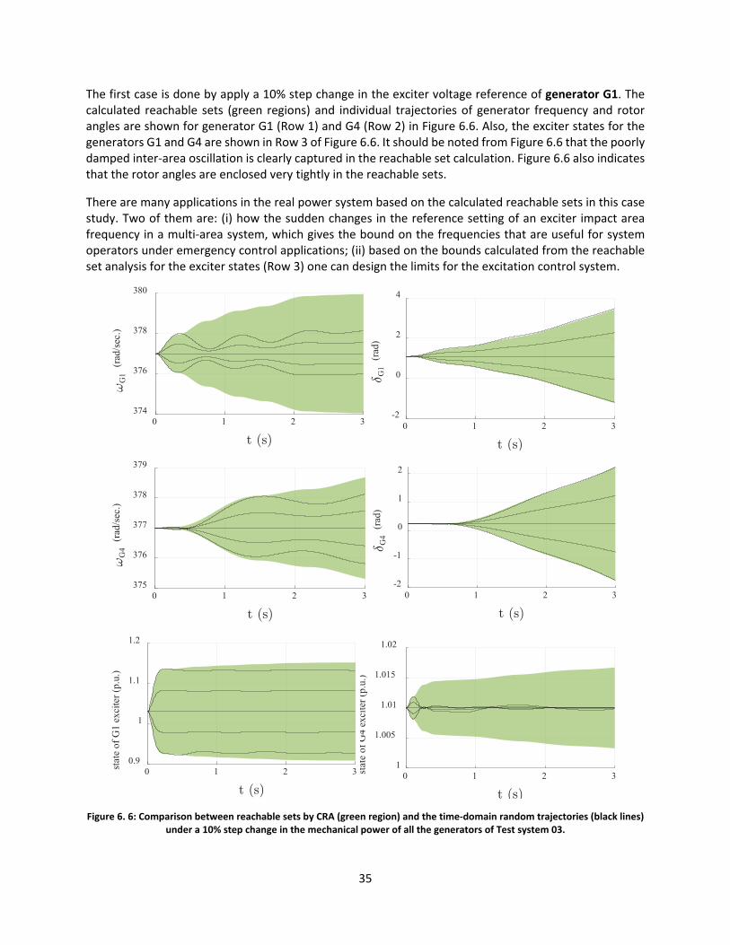
35

The first case is done by apply a 10% step change in the exciter voltage reference of generator G1. The calculated reachable sets (green regions) and individual trajectories of generator frequency and rotor angles are shown for generator G1 (Row 1) and G4 (Row 2) in Figure 6.6. Also, the exciter states for the generators G1 and G4 are shown in Row 3 of Figure 6.6. It should be noted from Figure 6.6 that the poorly damped inter-area oscillation is clearly captured in the reachable set calculation. Figure 6.6 also indicates that the rotor angles are enclosed very tightly in the reachable sets.

There are many applications in the real power system based on the calculated reachable sets in this case study. Two of them are: (i) how the sudden changes in the reference setting of an exciter impact area frequency in a multi-area system, which gives the bound on the frequencies that are useful for system operators under emergency control applications; (ii) based on the bounds calculated from the reachable set analysis for the exciter states (Row 3) one can design the limits for the excitation control system.

Figure 6. 6: Comparison between reachable sets by CRA (green region) and the time-domain random trajectories (black lines) under a 10% step change in the mechanical power of all the generators of Test system 03.

0 1 2 3374

376

378

380

G1

(rad

/sec

.)

0 1 2 3-2

0

2

4

G1

(rad

)

0 1 2 3375

376

377

378

379

G4

(rad

/sec

.)

0 1 2 3-2

-1

0

1

2

G4

(rad

)

0 1 2 30.9

1

1.1

1.2

stat

e of

G1

exci

ter (

p.u.

)

0 1 2 31

1.005

1.01

1.015

1.02

stat

e of

G4

exci

ter (

p.u.

)

36

Case 2: Under different levels of uncertainties in the mechanical power of generator G2.

Case 2 consists of a collection of scenarios that calculate the reachable sets of rotor angles, speeds, and tie-line current for different levels of uncertainties, i.e., 15%, 10%, and 5%, in the mechanical power of generator G2, respectively. The reachable sets of generator frequencies and rotor angles are shown for generators G2 (Row 1) and G3 (Row 2) in Figure 6.7. Also, reachable sets for the state variable of the current (real and imaginary) through one of the tie-lines between bus #7 and bus #8 (see Figure 6.5) are shown in Row 3 of Figure 6.7. It can be seen from Figure 6.7 that the envelopes of generator frequencies clearly capture the oscillatory behaviors of the test system under these disturbances.

The traditional contingency ranking for economic power dispatch is based on running extensive nonlinear time-domain simulations and is performed offline in planning studies. Planners consider an operating envelope and study credible uncertainties to ensure a reliable operation under worst-case scenarios. One obvious challenge comes from significant computational burden in running nonlinear time-domain simulations of realistic power system models while covering various uncertainties. However, performing reachable set analysis like the one in this case study provides operating limits (such as frequency limits as in Figure 6.7) of the grid components for a large horizon of uncertainties, which is very useful for reliable operation of a power system.

The thermal rating of the lines is one of the factors that limits the transmission capacity. Operating the transmission system with conservative margin (higher margin) will lead to inefficient utilization of scarce transmission resources. In many instances, it has restricted the transfer of renewable resources (e.g. wind and hydro) from remote locations to load centers. In today’s deregulated electricity market, operating the transmission system with lower transfer limits means increased cost for system operation, reduced social welfare, and increased congestion cost to the society. The thermal status of the tie-lines provided to the system operator as an operating guide. One of the main factors determines the thermal limits of a line is the current flow. The formal analysis can give us the maximum bound on the current for a given credible uncertainty as shown in the Row 3 of Figure 6.7.

0 0.5 1 1.5 2 2.5 3375

376

377

378

379

G2

(rad

/sec

.)

15% 10% 5%

0 0.5 1 1.5 2 2.5 3

-2

0

2

4

G2

(rad

)

15% 10% 5%

37

Figure 6. 7: Comparison between the reachable sets by CRA under different level (15%, 10%, and 5%) of undercities in the mechanical power of the generator G2 of Test System 03.

Case 3: Two types of uncertainties at the same time – (i) 10% step change in the mechanical power generator G1 and (ii) 5% step change in the exciter voltage reference of generator G4

In this case, two different type of disturbances are applied to the system in the same time. The two disturbances include a 10% step change in the mechanical power of generator G1 and a 5% step change in the exciter voltage reference of generator G4. The calculated reachable sets (green regions) and individual trajectories of generator frequency and rotor angles are shown for generator G1 (Row 1) and G3 (Row 2) in Figure 6.8. It can be observed from Figure 6.8 that the reachable sets consist of all random trajectories within its boundaries. This case study can be used to estimate the frequency bound of the test system under the occurrence of several disturbance at the same time.

0 0.5 1 1.5 2 2.5 3375

376

377

378

379

G3

(rad

/sec

.)

15% 10% 5%

0 0.5 1 1.5 2 2.5 3

-2

0

2

4

G3

(rad

)

15% 10% 5%

0 0.5 1 1.5 2 2.5 3-50

0

50

I7-

8 -

Imag

inar

y (p

.u.)

15% 10% 5%

0 0.5 1 1.5 2 2.5 3-40

-20

0

20

40

I7-

8 -

Rea

l (p.

u.)

15% 10% 5%

0 1 2 3 4 5374

376

378

380

G1

(rad

/sec.

)

0 1 2 3 4 5-5

0

5

10

G1

(rad

)

38

Figure 6. 8: Comparison between the reachable sets by CRA under different level (15%, 10%, and 5%) of undercities in the mechanical power of the generator G2 of Test System 03.

6.1.4 Test system 04: 16-machine system (relatively larger transmission system) Test system 04 is a commonly used model for a 16-machine, 68 bus example system [28], shown in Figure 6.9. This is a reduced-order equivalent of the interconnected New England test system (NETS) and New York power system (NYPS). There are five geographical regions, out of which NETS and NYPS are represented by a group of generators whereas, import from each of the three other neighboring areas, Area #3, Area #4 and Area #5 are approximated by equivalent generator models. Generators G1 to G9 are the equivalent representation of the NETS generation whilst, G10 to G13 represent the generation of the NYPS. Generators G14 to G16 are the dynamic equivalents of the three neighboring areas connected to the NYPS.

All generators are represented by their 8th order sub-transient model. The generators G1 to G8 are equipped with slow excitation systems (IEEE-DC1A) while G9 is equipped with a fast acting static excitation system (IEEE ST1A) and a speed-input power system stabilizer (PSS) to ensure adequate damping for its local modes. The rest of the generators are under manual excitation control.

0 1 2 3 4 5372

374

376

378

380

382

G3

(rad

/sec

.)

0 1 2 3 4 5

-5

0

5

10

G3

(rad

)

39

Figure 6. 9: Diagram for a modified 5-area 16-machine 68-bus system.

In the current GRA tool, the grid is modeled using ordinary differential equations (or electro-magnet transient or EMT type of models) because the reachability analysis converges better, especially for distributed FA, compared to the differential algebraic equation representation. There are 405 state variables in this test system. At presence, this EMT model does not include capacitive loads and line charging, and voltages are not state variables. On the other hand, the realistic system models all include such capacitive components. Therefore, to obtain a stable and feasible system (i.e., the power flow solves with reasonable voltage levels), some modifications had to be made to the original test system to adequate the modeling framework followed in this work.

These changes mainly include

(i) The line charging capacitors of the transmission lines and the tap changing ratio of the transformers are ignored

(ii) All the loads as well as shunts connected buses are assumed to be combined inductive and resistive

(iii) Real power from the generators are reduced to one-third its original value and the real powers of the load are also modified accordingly

(iv) Resistive values of the line impedance are assumed to larger than its original values

It needs to be pointed out that many trials were done before we have a reasonable system that can be used in this study. This is considered a limitation of the tool and will be corrected by developing full grid component models.

40

The case study is about a 50% step change in the mechanical power input at generator G16. The trajectories are shown for the 2 extreme cases (i.e. – 50% and +50% step change in the mechanical power), and the steady state. Figure 6.10 shows the speed of the generators representing each area of the test system (i.e. G1-Area #1, G13-Area #2, G14-Area #3, G15-Area #4, G16-Area #5). Again, Figure 6.10 shows that the individual trajectories are tightly enclosed in the corresponding reachable sets.

It should be noted that the oscillation modes typically observed in the original 16-machine test system is not observed in this case study. This is due to the modification made to the original test system data, which make the system overdamped.

One of the applications for this kind of exercises is to find out the bound on mechanical power of a specific generator for developing a Under frequency load shedding (UFLS) scheme. UFLS is an important means to tackle frequency drops caused by load-generation imbalance. In planning studies, system planners would be interested in finding the bound on the power generation limits of generating units, which leads to a UFLS. This type of study can be performed to develop an operating guide for system operators during decision making. Typically, this is done by the conventional Monte Carlo approach by performing a mass set of time-domain simulations using different samples. However, as shown in this case study, the reachable sets can give us very tight bounds on the frequency deviations of the area (i.e. Area #5) where the disturbances occur and other areas (e.g., Area #1, Area #2, Area #3, and Area #4) as well.

0 0.2 0.4 0.6 0.8 1

377

377.002

377.004

377.006

377.008

377.01

G1

(rad

/sec

)

0 0.2 0.4 0.6 0.8 1

377

377.002

377.004

377.006

377.008

377.01

G13

(rad

/sec

)

0 0.2 0.4 0.6 0.8 1377

377.002

377.004

377.006

377.008

377.01

G15

(rad

/sec

)

0 0.2 0.4 0.6 0.8 1377.0035

377.004

377.0045

377.005

377.0055

G14

(rad

/sec

)

0 0.2 0.4 0.6 0.8 1376.9

376.95

377

377.05

377.1

G16

(rad

/sec

)

41

Figure 6. 10: Comparison between reachable sets by CRA (green region) and the time-domain trajectories (black lines) under a 50% step change in the mechanical power G16 of Test system 04.

6.1.5 Test system 05 - 16-machine system with microgrids (Transmission and distribution system)

Figure 6.11 (a) shows the Transmission and Distribution (T&D) test system, where the transmission system is the 16-machine, 68 bus test system, like the one in test system 4 shown in Figure 6.9. To represent the distribution system, 2 identical microgrids are considered, see Figure 6.11 (b). These microgrids are connected to the transmission system at bus 68. The T&D system is interconnected through a ring network consisting of lines 1, 2, and 3, as shown Figure 6.11 (a). The same changes were made to the transmission system, as discussed in Section 6.3. There are 495 state variables in this test system in which 405 comes from the transmission network, 84 states from MG1 and MG2 (each consist of 42 states), and the rest represent the lines of the ring network.

Figure 6. 11: Transmission and distribution (T&D) system. (a) Schematic of T&D system; (b) schematic of the Microgrids MG1 and MG2.

The case study was performed by applying a 50% step change in the mechanical power of generator G16. The trajectories are shown for the 2 extreme cases (i.e. – 50% and +50% step change in the mechanical power), and the steady state. The following figures show the speed of the generators representing each area of the test system (i.e. G1-Area #1, G13-Area #2, G14-Area #3, G15-Area #4, G16-Area #5).

The trajectories are shown in Figure 6.12 for the 2 extreme cases (i.e. – 50% and +50% step change in the mechanical power), and the steady state. Row 1 shows the rotor speed of the generators G1, and G16 representing transmission system and the row 2 shows the rotor speed of the synchronous generator, real power generation of DG1 in MG1, and the real power generation of DG1 and DG2 in MG2.

42

Figure 6. 12: Comparison between reachable sets by CRA (green region) and the time-domain trajectories (black lines) for frequencies of G1, G16, MG1, and active power generation of DG1 in MG1 under a 50% step change in the mechanical power

G16 of Test system 05.

6.2 Distributed Reachability Analysis

As discussed in Section 3, a compositional scheme developed in [13] was applied to a microgrid case in [21]. While it was a viable approach, a significant amount of effort was spent on parameter tuning for convergence due to the interactions posed by the algebraic variables. The details can be found in [21] and will not be presented here. This section focuses on the DFA application to ODE representation of the power grid.

6.2.1 Test system 06 – Sequential DRA

Figure 6.13 (a) shows a networked microgrid consisting of three identical MGs. The detailed description of the MGs is shown in Figure 6.13 (b). The test system consists of three identical MGs, where each MG has two DGs, two loads and two lines, as shown Figure 6.13 (b). Three lines connect the MGs together, as indicated in Figure 6.13 (a). All these components together with the associated controls are modeled as described in Section 3.3.1. There are 108 state variables in this test system representing 34 state variables for each MGs and 6 for the lines connecting them.

The DRA scheme is applied to the system in this case study but performed sequentially. The test system is divided into three subsystems as MG1, MG2, and MG3. All these subsystems are modeled as an ODE system considering specific boundary conditions, as explained in Section 3.4.2. MG1 is considered the reference system with 𝑉𝑉𝑝𝑝𝑐𝑐𝑐𝑐 as input, and 𝐼𝐼𝑝𝑝𝑐𝑐𝑐𝑐 and 𝜔𝜔𝐴𝐴𝑒𝑒𝑓𝑓 as outputs. Whereas MG2 and MG3 are modeled as subsystems with 𝐼𝐼𝑝𝑝𝑐𝑐𝑐𝑐 and 𝜔𝜔𝐴𝐴𝑒𝑒𝑓𝑓 as inputs, and 𝑉𝑉𝑝𝑝𝑐𝑐𝑐𝑐 as output. The three lines connecting these three

0 0.2 0.4 0.6 0.8 1

377

377.002

377.004

377.006

377.008

377.01

G1

(rad

/sec

)

0 0.2 0.4 0.6 0.8 1376.9

376.95

377

377.05

377.1

G16

(rad

/sec

)

0 0.2 0.4 0.6 0.8 1377.002

377.003

377.004

377.005

377.006

377.007

SG in

MG

1(ra

d/se

c)

0 0.2 0.4 0.6 0.8 10.01298

0.013

0.01302

0.01304

0.01306

PD

G1

in M

G1(

p.u.

)

43

MGs are considered the backbone system, which interchanges the boundary variables between the reference system and the subsystems.

Figure 6. 13: (a) Schematic of the networked microgrids; (b) Schematic of detailed Microgrids.

The disturbance for this case study is the application of 5% step changes in active power reference signals at all the DGs at the same time. The reachable sets for various state variables including active power generation from the DGs is calculated. To verify the DRA analysis, the CRA is also performed on the same test system. Figure 6.14 shows the active power generation from the DGs representing each subsystem of the test system (MG1, MG2, MG3), shown in the first, second, and third row of the plots, respectively. Again, to validate that the reachable sets capture the trajectories for the disturbances within the given uncertainty range, a number of simulations were performed by randomly selecting the percentage change in active power reference, as indicated by the solid lines in Figure 6.14.

The following observations can be made from Figure 6.14

(i) all the random trajectories are within the bounds of the reachable sets for both CRA (purple line) and DRA (yellow region), which validates the effectiveness of both CRA and DRA on the test system;

(ii) the reachable sets calculated from the CRA (purple line) are a little more conservative than those for the DRA for most of the variables;

(iii) although the reachable sets by DRA are less conservative, they follow a similar pattern as those for the CRA, which validates the effectiveness of DRA;

(iv) the reachable sets calculated by DRA (yellow region) are within the region of CRA (purple line) for most of the time.

It should be noted from Figure 6.14 that the reachable boundaries calculated from the DRA are tighter that the CRA. In this case study, the possible causes for this difference are: (i) the reachable sets of the interface states from the reachable sets of other subsystems is obtained with a specified threshold to ensure convergence; (ii) the derivatives of the interface variable are ignored (i.e. the last term in Equation (3.10) is ignored). However, the DRA provides a tighter bound on the variable, which is indeed beneficial for power system applications.

44

Figure 6. 14: Comparison between reachable sets by CRA (purple lines), DRA (yellow region) and the time-domain

trajectories (black lines) under a 5% step change in Pref of all the DGs of Test system 06.

6.2.2 Parallelization of the DRA Using Multi-core

As discussed in Section 3, one of the advantages with the DRA is that it enables the parallel implementation of formal analysis of more complicated power grids. To verify this, the DRA scheme for the above test case was implemented for parallel computation in a MATLAB® platform using the Parallel Computing Toolbox [29]. As indicated by the DRA algorithm in Section 3.5, only Step 4, i.e., the reachable sets calculation for Subsystems 2 𝑡𝑡𝑐𝑐 𝑐𝑐 can be parallelized. The reference system, usually Subsystem 1, is analyzed followed by the parallel computation of reachable sets for other subsystems in every iteration, and the data are then exchanged between the reference system and the other subsystems. The parallelization of evaluating other subsystems can be implemented using the parallel for-loop computation (‘parfor’ in MATLAB®).

The simulation was carried out using both CRA and DRA on the same test system to perform a reachable sets calculation for 0.5 seconds with a time step size of 5×10-4 seconds. All the computations were performed on a windows computer with an Intel Core i7 (8th generation) processor and 64GB of RAM. The reachability analyses for Subsystems 2 and 3 were distributed to two cores of the processor. For the above case study, the total computational time for CRA was 1,650.3 seconds, 1972.5 seconds for

0 0.1 0.2 0.3 0.4 0.51.65

1.7

1.75

1.8

PD

G1

in M

G1

(p.u

.)

0 0.1 0.2 0.3 0.4 0.51.65

1.7

1.75

PD

G2

in M

G1

(p.u

.)0 0.1 0.2 0.3 0.4 0.5

1.65

1.7

1.75

1.8

PD

G1

in M

G2

(p.u

.)

0 0.1 0.2 0.3 0.4 0.51.65

1.7

1.75

PD

G2

in M

G2

(p.u

.)

0 0.1 0.2 0.3 0.4 0.5

1.65

1.7

1.75

1.8

PD

G1

in M

G3

(p.u

.)

0 0.1 0.2 0.3 0.4 0.51.65

1.7

1.75

1.8P

DG

2 in

MG

3 (p

.u.)

45

sequential DRA, and 3,334.9 seconds for the distributed DRA. The following are possible reasons for DRA not having an advantage over the CRA computational time:

• Data exchange has to be explicitly performed in sequential and parallel DRAs while the data are shared in the CRA. This is the reason that DRAs are taking more time to complete.

• The ‘parfor’ implementation in the MATLAB® toolbox utilizes multiple cores of the computer machine known as ‘workers,’ which can execute the long iterations simultaneously and the main core which executes the major code is known as the ‘client’. During the execution of a parallel for-loop there will be data exchange between the client and the workers. This data exchange can dominate the execution time of the DRA if the study system is small, that is the case in this case study. This data exchange between different cores by workers contributes to the longer computation time taken by the parallel DRA.

• The computational complexity of the CRA is 𝒪𝒪(2𝑛𝑛�𝑐𝑐5), where 𝑐𝑐� is the total number of variables in the nonlinear terms of the nonlinear system and 𝑐𝑐 is the total number of differential and algebraic variables. If the nonlinearity is not very strong, the computational complexity can be reduced to 𝒪𝒪(𝑐𝑐3). Therefore, if the study system is not very large the advantage of reduction in computational complexity may not be observed, and the overhead caused by the data exchange can be significant. This is another contributor to the longer computation time of the parallel DRA.

• Reachability analysis of only two subsystems can be computed in parallel in this test system. The reduction in dimensions is insufficient to reduce the total computation time in the DRA case.

Currently, we do not have a suitable system for this test. This issue will be further investigated in the extension of the project.

6.3 Data-Driven Reachability Analysis

The networked microgrids in Figure 4.1 are used for this study. The test system consists of 4 microgrids, 5 DERs and 1 synchronous generator, and Microgrid 4 is the external system. Two cases were studied with a slight change and a large change in the load, respectively. The DDFA results are presented in Figures 6.15 (the slight change) and 6.16 (the large change).

46

Figure 6. 15: DDFA for a slight load change.

The data-driven reachable sets and some trajectories for DG1 real and reactive power generation are shown in Row 1 of Figure 6.15. The trajectories are enclosed in the reachable sets while the generators are regulating the output to deal with the load variation. The second row in Figure 6.15 shows the plots for the data-driven (in green) and the model-based reachable sets (in red), which match very well, for the DG1 outputs.

Figure 6.16 shows the same plots for a large load variation scenario.

47

Figure 6. 16: DDFA for a large load change.

48

7. Conclusions and Future Work In this study, the reachability analysis for nonlinear dynamic systems was introduced into power grid studies. A generic MATLAB® based grid reachability analysis (GRA) tool was developed to conduct both centralized, distributed, and data-driven formal analyses for typical transmission and/or distribution networks under various disturbances. Starting from a FA toolbox, CORA, the electro-magnetic transient (EMT) type models of generic grids were built by developing and integrating dynamics for various grid components including synchronous generators, power system stabilizers (PSSs), exciters, turbine governors, distributed generators (DGs), controls etc. Numerical algorithms were developed for computing Jacobian and Hessian matrices for the FA computation of generic systems. A distributed scheme was developed to parallelize the reachable set computation, especially for ODE representation of power systems. The FA tool for the grid takes input data files for transmission and/or distribution networks, formulates the EMT model, and performs reachable set computation in a centralized or distributed manner. Case studies were performed using both transmission and distribution systems including networked microgrids.

As indicated previously, this report does not repeat work that has been published previously, which mainly included the DFA for DAE representation of the grid using a compositional scheme and its parallelization. It also includes a discussion of the quasi diagonalization-based Geršgorin theory [21] and the reachable set computation for large disturbances, i.e., faulted scenarios [30].

As a follow-up to the original project scope, additional studies are being performed to further refine the open-source FA tool. In the FA application and the tool implementation, various transmission and distribution components are modeled, including synchronous generators and their associated controls, as well as distributed generators such as solar generation with their controls. A unified data format was defined for the efficient study of integrated transmission and distribution systems. In the current tool, the grid is modeled using ordinary differential equations (or electro-magnet transient or EMT type of models) because the reachability analysis converges better, especially for distributed FA, compared to the differential algebraic equation representation. Currently, this EMT does not model capacitive loads and line charging. To make the FA tool complete, additional work is being performed to further include capacitive effects.

In the EMPT models, the states include the differential variables representing the generator inertial dynamics and controllers and transmission lines. Line currents are state variables while voltages are algebraic variables that will be absorbed. In addition to the line currents, the voltages associated with line charging or capacitive components also become the states, and the currents through the capacitive components become algebraic variables. The modeling of such components needs to be included in the FA tool by incorporating both KCL and KVL laws before performing the reachability analysis.

The additional models for capacitive components particularly impact the distributed FA since in the current DFA scheme, the input (output) is either the current (states) or voltage (algebraic variables) in different subsystems. The DFA scheme needs to be modified to accommodate the exchange of input (output) consisting of both voltage and current information at the boundary of the subsystems. The new DFA scheme will be developed and implemented in the FA toolset.

49

References: [1] H.-D. Chiang, “Direct methods for stability analysis of electric power systems: theoretical foundation, BCU methodologies, and applications,” John Wiley & Sons, March 16, 2013.

[2] E. Asarin, T. Dang, G. Frehse, A. Girard, C. Le Guernic, and O. Maler, “Recent progress in continuous and hybrid reachability analysis,” in Proc. of the 2006 IEEE Conference on Computer Aided Control Systems Design, 2006, pp. 1582–1587

[3] Goran Frehse, An Introduction to Hybrid Automata, Numerical Simulation and Reachability Analysis, Formal Modeling and Verification of Cyber-Physical Systems, DOI 10.1007/978-3-658-09994-7_3, Springer Fachmedien Wiesbaden 2015.

[4] G. Frehse, “PHAVer: Algorithmic verification of hybrid systems past HyTech.” in HSCC’05, vol. 3414 in LNCS. Springer, 2005, pp. 258–273.

[5] T. A. Henzinger, P.-H. Ho, and H. Wong-Toi, “HYTECH: A model checker for hybrid systems.” STTT, vol. 1, no. 1-2, pp. 110–122, 1997.

[6] J. Maidens and M. Arcak, “Reachability Analysis of Nonlinear Systems Using Matrix Measures,” IEEE TRANSACTIONS ON AUTOMATIC CONTROL, VOL. 60, NO. 1, JANUARY 2015

[7] E. A. Cross and I. M. Mitchell, “Level set methods for computing reachable sets of systems with differential algebraic equation dynamics,” in Proc. Amer. Control Conf., 2008, pp. 2260–2265.

[8] I. M. Mitchell and Y. Susuki, “Level set methods for computing reachable sets of hybrid systems with differential algebraic equation dynamics,” in Hybrid Systems: Computation and Control. New York, USA: Springer, 2008, vol. 4981, Lecture Notes in Computer Science, pp. 630–633.

[9] L. Jin, R. Kumar, and N. Elia, “Reachability analysis based transient stability design in power systems,” Electrical Power and Energy Systems 32 (2010) 782–787

[10] L. Jin, H. Liu, R. Kumar, J.D. McCalley, N. Elia, and V. Ajjarapu, “Power system transient stability design using reachability based stability-region computation,” Proceedings of the 37th Annual North American Power Symposium, 2005.

[11] T. Dang, A. Donze, and O. Maler, “Verification of analog and mixed signal circuits using hybrid systems techniques,” in Formal Methods for Computer Aided Design. New York, NY, USA: Springer, 2004, vol. 3312, Lecture Notes in Computer Science, pp. 21–36.

[12] M. Althoff and B. H. Krogh, “Reachability Analysis of Nonlinear Differential-Algebraic Systems,” IEEE Transactions on Automatic Control, Vol. 59, No. 2, FEBRUARY 2014.

[13] A. El-Guindy, Y. Chen, and M. Althoff, “Compositional Transient Stability Analysis of Power Systems via the Computation of Reachable Sets,” 2017 American Control Conference, May 24–26, 2017, Seattle, USA.

[14] Oded Maler, Computing Reachable Sets: An Introduction

[15] Matthias Althoff, Reachability Analysis and its Application to the Safety Assessment of Autonomous Cars, Doctor’s dissertation submitted to Technischen Universit at Munchen.

50

[16] J. K. Scott, D. M. Raimondo, G. R. Marseglia, and R. D. Braatz, Constrained zonotopes: A new tool for set-based estimation and fault detection, Automatica, Volume 69, July 2016, Pages 126-136.

[17] W. Kuhn, “Rigorously computed orbits of dynamical systems without the wrapping effect.” Computing, vol. 61, pp. 47–68, 1998.

[18] A. Girard. Reachability of uncertain linear systems using zonotopes. In Hybrid Systems: Computation and Control, LNCS 3414, pages 291–305. Springer, 2005.

[19] A. Girard, C. Le Guernic, and O. Maler. Efficient computation of reachable sets of linear time-invariant systems with inputs. In Hybrid Systems: Computation and Control, LNCS 3927, pages 257–271. Springer, 2006.

[20] M. Althoff and B. H. Krogh, "Zonotope bundles for the efficient computation of reachable sets," 2011 50th IEEE Conference on Decision and Control and European Control Conference, 2011, pp. 6814-6821

[21] Y. Li, P. Zhang, M. Althoff, and M. Yue, “Distributed Formal Analysis for Power Networks with Deep Integration of Distributed Energy Resources”, IEEE Transactions on Power Systems, Volume: 34, Issue: 6, Nov. 2019.

[22] P. Kundur, NJ Balu, MG Lauby, Power system stability and control, ser. The EPRI power system engineering series. New York; London: McGraw-Hill, 1994.

[23] N. Pogaku, M. Prodanovic and T. C. Green, "Modeling, Analysis and Testing of Autonomous Operation of an Inverter-Based Microgrid," in IEEE Transactions on Power Electronics, vol. 22, no. 2, pp. 613-625, March 2007.

[24] Y. Zhou, P. Zhang, and M. Yue, “An ODE-Enabled Distributed Transient Stability Analysis for Networked Microgrids,” IEEE PES GM 2020.

[25] Y. Zhou and P. Zhang, “Data-Driven Formal Analysis for Dynamic Power Networks,” An internal report, November 20, 2020.

[26] S. B. Liu and M. Althoff, “Reachset conformance of forward dynamic models for the formal analysis of robots,” in 2018 IEEE/RSJ International Conference on Intelligent Robots and Systems (IROS), pp. 370–376, IEEE, 2018.

[27] M. Althoff and N. Kochdumper, “Cora 2018 manual.” url: http://engineering.purdue.edu/ mark/puthesis.

[28] B. Pal and B. Chaudhuri, Robust Control in Power Systems (Power Electronics and Power Systems). New York, NY, USA: Springer, 2005., Volume: 34, Issue: 6, Nov. 2019.

[29] https://www.mathworks.com/products/parallel-computing.html#see-parallel-computing-toolbox-in-action

[30] Y. Zhou, P. Zhang, and M. Yue, “Reachable dynamics of networked microgrids with large disturbances,” IEEE Transactions on Power Systems, accepted, Oct. 2020.

51

Appendix A: Input data Format

The GRA toolbox is developed for generic power systems. For this purpose, the input data of the system follows a specified format that is similar to the one defined in power system tools (e.g. Power System Toolbox (PST)-toolbox). To facilitate the study of both transmission and distribution systems (microgrids), the DG data are defined separately from the synchronous generator data.

The following are the description of the data input format (Data_file.m) for each of the power system components considered in this toolbox.

SG data

%%%%%%%%%%%%%%%%% Machine data format 1. machine number, 2. bus number, 3. base mva, 4. leakage reactance x_l(pu), 5. resistance r_a(pu), 6. d-axis synchronous reactance x_d(pu), 7. d-axis transient reactance x'_d(pu), 8. d-axis sub-transient reactance x"_d(pu), 9. d-axis open-circuit time constant T'_do(sec), 10. d-axis open-circuit sub-transient time constant T"_do(sec), 11. q-axis synchronous reactance x_q(pu), 12. q-axis transient reactance x'_q(pu), 13. q-axis sub-transient reactance x"_q(pu), 14. q-axis open-circuit time constant T'_qo(sec), 15. q-axis open circuit sub-transient time constant T"_qo(sec), 16. inertia constant H(sec), 17. damping coefficient d_o(pu), 18. Terminal voltage Vt (pu), 19. Mechanical power Tm (pu), 20. Machine subsystem Number 21. Machine type (1- sub-transient, 0-for electromechanical model)

Exciter data

%%%%%%%%%%%%%%%%% exciter data format 1 - exciter type (0 for manual, 1 for ST1A, 2 for DC1A) 2 - machine number 3 - input filter time constant T_R 4 - voltage regulator gain K_A 5 - voltage regulator time constant T_A 6 - exciter constant K_E 7 - exciter time constant T_E 8 - saturation function Aex 9 - saturation function Bex 10- stabilizer gain K_F 11 - stabilizer time constant T_F 12 – Exciter voltage reference V_ref

52

PSS data

%%%%%%%%%%%%%%%%% Power System Stabilizer data format % 1 - PSS number % 2 - Machine number (PSS location) % 3 - Washout time constant (Tw) % 4 - lead-leg block time constant 1 (T1) % 5 - lead-leg block time constant 2 (T2) % 6 - lead-leg block time constant 3 (T3) % 7 - lead-leg block time constant 4 (T4) % 8 - Gain (K_pss) % 9 - Maximum limit on the output % 10 - Minimum limit on the output % 11 – Measurement delay (T_m)

Load data

%%%%%%%%%%%%%%%%%%% MG Load data format 1. load number, 2. BUS number, 3. r - (pu) resistive load 4. l - (pu) inductive load 5. load subsystem Number Line Data

%%%%%%%%%%%%%%%%% MG line data format 1. line number 2. from bus 3. to bus 4. r_line - (pu) resistance 5. x_line - (pu) inductive 6. Line subsystem Number

DG data

%%%%%%%%%%%%%%%%% DG data format 1. DG number 2. BUS number 3. Pref (pu)- Power reference 4. Pn (W)- P nominal 5. Qn (Var)- Q nominal 6. Vn (pu)- V nominal 7. omega_n (pu) – nominal frequency 8. omega_c (Hz)-cut-off frequency of low-pass filters 9. Cf - (pu) AC side filter capacitor 10. Lf - (pu)AC side filter inductor 11. Rf -(pu) AC side filter resistance

53

12. Lc - (pu) coupling inductor 13. rc - (pu) coupling resistance 14. fs - (Hz)Switching frequency 15. - DG subsystem Number DG control parameters

%%%%%%%%%%%%%%%%% DG control parameters format

1. DG number 2. mp - P-F droop coefficient 3. nq - Q-V droop coefficient 4. kpv - voltage controller Proportional gain 5. kiv - voltage controller Integral gain 6. kpc - Current controller Proportional gain 7. kic - Current controller Integral gain 8. F - current feed-forward gain