Foreword

Pressurized irrigation systems working on demand were the object of considerable attention inthe sixties and seventies and a considerable number of them were designed and implemented inthe Mediterranean basin mainly but also in other parts of the world. They offer a considerablepotential for efficient water use, reduce disputes among farmers and lessen the environmentalproblems that may arise from the misuse of irrigation water. With the strong competition that isarising for the water resources, modernization of irrigation systems is becoming a critical issueand one of the alternatives to modernize is the use of pressurized systems to replace part of theexisting networks. This approach is being actively pursued in many countries.

Much of the work done in the past concentrated in the design and optimization of such systemsand FAO through its Irrigation and Drainage Paper 44: "Design and optimization of irrigationdistributions networks" (1988) contributed substantially to this area of knowledge. However,practically no tool existed to analyse the hydraulic performance of such systems, which are verycomplex due to their constantly varying conditions, until few years ago where the new computergenerations permitted complex simulations.

The present work was started with the idea of developing such tool based in the great capacityof computers to generate randomly many situations which could be analysed statistically andprovide clear indications of where the network was not functioning satisfactorily. However thiswork put rapidly in evidence that the same criteria could also be used to analyse a networkdesigned according to traditional criteria and improve the design. This led to the conclusion thatthe design criteria also needed revision and this additional task was also faced and completed.

The present publication, therefore, has as its main objective the development of a computer toolthat permits the diagnosis of performance of pressurized irrigation systems functioning ondemand (also under other conditions), but also provides new and revised criteria for the designof such irrigation networks. The publication intends to be complementary to Irrigation andDrainage Paper 44 and where necessary the reader is referred to it for information ormethodologies that are still valid.

An effort has been made to reduce the development of formulae but the subject is complex andtheir use is unavoidable. Calculations examples have been included to demonstrate thecalculation procedures and facilitate the understanding and practical use of formulae. Thecomputer program (COPAM) performs these calculations in a question of seconds but it isimportant that the user has full understanding of what is being done by the program and has thecapacity to verify the results.

The computer model has been tested in several field situations in the Mediterranean basin. It hasproved its usefulness not only by quickly identifying the weak points of the network but also byidentifying the power requirements of pumping stations needed to satisfy varying demandsituations and often proving that the powerhouses were not well suited (overdesigned orunderdesigned) to meet the requirements of the network.

The present publication is intended to provide new methods for the design and analysis ofperformance of pressurized irrigation systems, and should be of particular interest to districtmanagers, consultants irrigation engineers, construction irrigation companies, universityprofessors and students of irrigation engineering and planners of irrigation systems in general.

iv

Comments from potential users are welcomed and should be addressed to:

ChiefWater Resources, Development and Management ServiceFAO, Viale delle Terme di Caracalla00100 Rome, Italy

or to

ChiefHydraulic Engineering ServiceCIHEAM – Bari InstituteVia Ceglie 9, 70010 Valenzano (Bari), Italy.

Performance analysis of on-demand pressurized irrigation systems v

Acknowledgements

The past involvement of FAO in the subject of this publication, the potential that the subjectoffers for the future modernization of irrigated agriculture and the interest and experience of theCIHEAM in this area have made it particularly suitable for the association of both organizationsin the preparation of this publication, which was of mutual interest.

The author wishes to acknowledge the Director of CIHEAM-Bari Institute and the Director ofthe Land and Water Development Division of FAO for the continuous support to theundertaking of this activity.

Special mention is due to several students who have participated over the years in theEngineering Master courses at the CIHEAM-Bari Institute and have contributed to the evolutionof the modelling approaches presented in this paper.

Special thanks are due to L.S. Pereira, Professor at the Technical University of Lisbon(Portugal) and to M. Air Kadi, Secretary General at the Ministry of Agriculture of Rabat(Morocco) who have been the source of constant inspiration and advice.

Special thanks are also due to the reviewers of the publication, Messrs J.M. Tarjuelo, Professorof the University of Castilla-La Mancha, Spain, T. Facon, Technical Officer, FAO RegionalOffice for Asia and the Pacific, and R.L. Snyder, Professor, University of California.

This work is dedicated to the memory of Yves Labye who contributed greatly to the scientificbackground of the approaches used in the present paper and whose works still remain anoutstanding intellectual reference.

vi

Performance analysis of on-demand pressurized irrigation systems vii

Contents

page

1 ON-DEMAND IRRIGATION SYSTEMS AND DATA NECESSARY FOR THEIR DESIGN 1

Main criteria to design a distribution irrigation system 2Layout of the paper 6

2 NETWORK LAYOUT 9

Structure and layout of pressure distribution networks 9Design of an on-demand irrigation network 9

Layout of hydrants 9Layout of branching networks 9

Optimization of the layout of branching networks 10Methodology 10Applicability of the layout optimization methods 13

3 COMPUTATION OF FLOWS FOR ON-DEMAND IRRIGATION SYSTEMS 15

One Flow Regime Models (OFRM) 16Statistical models: the Clément models 16The first Clément model 16The second Clément model 32

Several Flow Regimes Model (SFR Model) 39Model for generating random discharges 39

4 PIPE-SIZE CALCULATION 43

Optimization of pipe diameters with OFRM 43Review on optimization procedures 43Labye's Iterative Discontinuous Method (LIDM) for OFR 45

Optimization of pipe diameters with SFRM 54Labye's Iterative Discontinuous Method extended for SFR (ELIDM) 55Applicability 58

The influence of the pumping station on the pipe size computation 58The use of COPAM for pipe size computation 59

Sensitivity analysis of the ELIDM 63

5 ANALYSIS OF PERFORMANCE 67

Analysis of pressurized irrigation systems operating on-demand 67Introduction 67Indexed characteristic curves 67Models for the analysis at the hydrant level 79Reliability indicator 92

viii

6 MANAGEMENT ISSUES 97

Some general conditions for a satisfactory operation of on-demand systems 97Suitable size of fa mily holdings 97Medium to high levels of irrigation and farm management knowledge 97Volumetric pricing 98Correct estimation of the design parameters 98Reduced energy costs 98Qualified staff for the operation and maintenance of the system 99

The on-demand operation during scarcity periods 99Volumetric water charges 101Water meters 102Types of volumetric charges 102Recovery of investments through the volumetric charge 103The operation, maintenance and administration costs 103The maintenance of the pumping stations and related devices 104

Flow and pressure meters: 104Pumps: 104Compressors: 105Switchboards: 105Ancillary works: 105

The maintenance of the irrigation network 105Towards the use of trickle irrigation at the farm level in on-demand irrigation systems 105New trends and technologies of delivery equipment 106

BIBLIOGRAPHY 109

ANNEX 1 VALIDATION OF THE 1ST CLÉMENT MODEL 115

ANNEX 2 PIPE MATERIALS AND DESIGN CONSIDERATIONS 125

ANNEX 3 EXAMPLE OF INPUT AND OUTPUT FILES 131

Performance analysis of on-demand pressurized irrigation systems ix

List of figures

page

1. Scheme of the main steps of an irrigation project 42. The chronological development process of an irrigation system 53. Sound development process of an irrigation system 64. Synthetic flow chart of COPAM 75. Proximity layout: application of Kruskal’s algorithm 116. Proximity layout: application of Sollin’s algorithm 117. 120° layout – case of three hydrants 118. 120° layout – case of four hydrants 129. 120° layout – case of four hydrants (different configuration) 1310. Variation of the elasticity of the network, eR, versus the total number of hydrants for different

values of r and eh, for U(Pq) = 1.645 2011. COPAM icon 2412. First screen of the COPAM package 2413. Layout of the COPAM package 2514. File menu bar and its sub-menu options 2515. Edit menu bar and its sub menu items 2616. Sub menu Edit/Hydrants discharge 2717. Examples of node numbering 2818. Edit/network layout sub-menu 2919. Edit list of pipes sub-menu 3020. Edit description sub-menu 3021. Toolbar button “Check input file” 3122. Clément parameters: 1st Clément formula 3223. Diagram representing u' as a function of F(u') 3424. Clément parameters: 2nd Clément formula 3725. Comparison between discharges computed with the 1st and the 2nd Clément equations applied

to the Italian irrigation network illustrated in Annex 1 3826. Probability of saturation versus the 1st Clément model discharges 3827. Operation quality, U(Pq) versus the 2nd Clément model discharges 3928. Typical layout of a network 4029. Random generation program 4130. Random generation parameters 4231. Characteristic curve of a section 4632. Characteristic curve of a section 4733. Elementary scheme 5534. Costs (106 ITL) of the network in the example, calculated by using the ELP and the ELIDM

for different sets of flow regimes 5835. Optimization of the pumping station costs 5936. Pipe size computation program 6037. Optimization program: “Options” Tab control 6038. Optimization program: “Mixage”Tab control 61

x

page

39. Optimization program: “Data” Tab control 6240. Input file: Edit network layout 6241. Optimization program: “Options” Tab control 6342. Optimization program: “Data” Tab control 6443. Optimization program: “Options” Tab control 6444. Layout of the network 6545. Cost of the network as a function of the number of configurations. The average costs and the

confidence interval concern 50 sets of discharge configurations. 6646. Characteristic curve of a hydrant 6847. Characteristic curve of a hydrant 6948. Characteristic curves program 7049. Characteristic curves program: parameters of the analysis 7150. Input file: edit network layout 7251. Graph menu bar and sub-menu items 7252. Open file to print the characteristic curves 7353. Indexed characteristic curves of the irrigation system under study 7454. Scheme of a pumping station equipped with variable speed pumps 7655. Characteristic curves of variable speed pumping station and the 93% indexed characteristic

curve of the network 7756. Power required by the plant equipped with variable speed pumps (type A) and a classical

plant (type B), as a function of the supplied discharges 7757. Indexed characteristic curves for the Lecce irrigation network computed using 500 random

configurations 7858. Flow chart of AKLA 8159. Curves representative of the percentage of unsatisfied hydrants (PUH) versus the discharge,

for different probabilities for PUH to be exceeded 8260. Curves representative of the upstream piezometric elevation (Z0,1<Z0,2<Z0,3<Z0,4) with the

variation of the percentage of unsatisfied hydrants (PUH), for an assigned probability ofoccurrence 82

61. Curves representative of the percentage of unsatisfied hydrants (PUH) with the variation ofthe upstream piezometric elevation (Z0,1<Z0,2<Z0,3<Z0,4), for an assigned probability ofoccurrence 83

62. Relative pressure deficits for every hydrant in the network 8363. Relative pressure deficits for every hydrant in the network 8464. Hydrants analysis program: “Options” Tab control, “Several-random generation” flow

regime 8465. Hydrants analysis program: “Options” Tab control, “Several-read from file” flow regime 8566. Hydrants analysis program: “Set point” Tab control 8667. Hydrant analysis program: “Elevation-discharge” Tab control 8668. “Graph” menu bar and sub-menu items 8769. Indexed characteristic curves for the irrigation network under study, computed using 500

random hydrants configurations 8870. Curves of the probabilities that a given percentage of unsatisfied hydrants (PUH) be

exceeded, computed using 500 random configurations. Upstream elevation Z0= 81.80 ma.s.l 89

71. Curves representative of the percentage of unsatisfied hydrants (PUH), with 10% ofprobability to be exceeded, with the variation of the upstream piezometric elevation from60 up to 110 m a.s.l. 90

Performance analysis of on-demand pressurized irrigation systems xi

72. Relative pressure deficits at each hydrant when 500 discharge configurations were generated.Discharge Q0=675 l s -1 and upstream piezometric elevation Z0=81.80 m a.s.l 91

73. Variation of the relative pressure deficit at each hydrant in each discharge configuration 9174. Analysis with 200 random configurations of 50 l s -1 9475. Analysis with 200 random configurations of 60 l s -1 9576. Relative pressure deficits obtained with the model AKLA and 90% envelope curves.

Analysis of the networks with 200 random configurations of 50 l s -1 9577. Relative pressure deficits obtained with the model AKLA and 90% envelope curves.

Analysis of the networks with 200 random configurations of 60 l s -1 9678. Typical demand hydrographs at the upstream end of an irrigation sector: a) on-demand

operation; b) arranged demand operation 10079. Cross-section of a hydrant 10380. Scheme of a delivery device controlled by an electronic card 107

List of tables

page

1. Standard normal cumulative distribution function 182. Discharges flowing into each section of the network under study (output of the COPAM

package: computation with the first Clément model) 213. Discharges flowing into each section of the network under study (output of the COPAM

package: computation with the second Clément model) 374. Elementary scheme 575. Comparing the power requirements for a pumping plant equipped with variable speed pumps

(type A) and for a classical pumping plant (type B), as a function of the discharges supplied 75

xii

List of symbols

A irrigated area [ha]

C number of configurations [ ]

CRK

number of combinations of R hydrants taken K at a time [ ]

d nominal discharge of the hydrant [l s 1− ]

dH variation of the head at the upstream end of the elementary scheme of the network [m]

dj discharge for supplying the network downstream the hydrant j [l s-1]

dP minimum cost variation [ITL]

dYk variation of the friction losses in section k [m]

D diameter of the pipe [mm]

Dck commercial diameters for section k [mm]

(Dmax)k maximum commercial diameter for the section k [mm]

(Dmax)k,r maximum commercial diameter of the section, k, for the configuration r [mm]

(Dmin)k minimum commercial diameter for the section k [mm]

(Dmin)k,r minimum commercial diameter of the section, k, for the configuration r [mm]

ΕΗi minimum value of the excess head prevailing at all the nodes where thehead changes [m]

f input frequency of the network (50 Mz standard) [Mz]

F set of all unsatisfactory states (failure) [ ]

F(u') ratio between Ψ(u') and Π(u') [ ]

Fh cumulated frequency of the hourly withdrawals during the peak period [ ]

FPSE empirical function indicating the cost variation of the sectors' network, SE,for the variation of its upstream piezometric elevation (ZSE ) [ ]

g acceleration of gravity [m s-2]

Hj,r head of each hydrant j within the configuration r [m]

(H j)r head of the whole set of hydrants j within the configuration r [m]

Performance analysis of on-demand pressurized irrigation systems xiii

Hj,min minimum head required at the hydrant j [m]

Hj head at the hydrant j [m]

Hmin minimum required head [m]

Ho hydrostatic head [m]

HPS head at the pumping station [m]

ITL Italian lire [ ]

J generic slope of the piezometric line [m m-1]

Jk,s head losses for unit length of the section k, with the diameter Ds [m m-1]

Jk,s,r head losses for unit length of the section k, for the discharge of the configuration r, with the diameter Ds [m m-1]

k section identification index [ ]

L generic length of the section [m]

Lk length of the section k [m]

Ls,k length of the sth diameter of the section k [m]

N number of hydrants simultaneously operating [ ]

NADk number of allowable commercial diameters for the section k [ ]

NADk number of allowable diameters for the section k [ ]

Np total population of withdrawn discharges [ ]

NQi number of discharges included in the class i [ ]

NSE number of sectors within the district to be optimized [ ]

NTR total number of sections [ ]

p elementary probability of operation of each hydrant [ ]

PC average cost of the network for the configurations C [ITL]

PGλ conditional probability to change from the state j into the state j+1 during the interval dt [ ]

PGµ conditional probability to change from the state j into the state j-1during the interval dt [ ]

Pi,C cost of the network for the configurations i of C [ITL]

Pk cost of the section k [ITL]

Pλ conditional probability for having an arrival during the time interval (t, t+dt) [ ]

xiv

Pµ conditional probability for having a departure during the time interval (t, t +dt) [ ]

PNET cost of the network [ITL]

Pq cumulative probability [ ]

Ps cost per unit length of diameter Ds [ITL m-1]

PSAT conditional probability to have saturation when an opening occurs [ ]

qp peak continuous flow rate 24/24 hours on the total area [l s-1ha-1]

qpi peak continuous flow rate 24/24 hours on the irrigable area [l s-1ha-1]

qs specific continuous discharge [l s-1ha-1]

Q average discharge withdrawn during the peak period [l s-1]

Q generic discharge [l s-1]

QCl Clément discharge at the upstream end of the network [l s-1]

Qh,d hourly discharges recorded during the peak period [l s-1]

Qk discharge in the section k [l s-1]

Qk,r discharge flowing in the section k for the configuration r [l s-1]

Qt discharge withdrawn at a generic instant t at the upstream end of the network [l s-1]

Qt+t1 discharge withdrawn at an instant t+t1at the upstream end of the network [l s-1]

r coefficient of utilization of the network [ ]

R total number of hydrants [ ]

Re number of Reynolds [ ]

RN random number having uniform distribution function [ ]

s j numerical indicator of the severity of the state xj of a system [ ]

S set of all satisfactory states [ ]

Sk series of commercial diameters for each section, k, between (Dmin)k and (Dmax)k [ ]

t' average operation time of each hydrant during the peak period [h]

tirr duration of the opening of the hydrant j [h]

T f average sojourn time in the failure states during the period under observation [h]

T duration of the peak period [h]

T' operating time of the network during the period T [h]

Performance analysis of on-demand pressurized irrigation systems xv

Tf time period in which the system is in unsatisfactory state [h]

u dimensional coefficient of resistance [m-1 s2 ]

u standard normal variable in the 1st Clément's formula [ ]

u' standard normal variable in the 2nd Clément's formula [ ]

U(Pq) standard normal variable for P = Pq [ ]

vmax maximum flow velocity [m s-1]

vmin minimum flow velocity [m s-1]

Vd average daily volume [m3]

Vh average hourly volume [m3]

VT total average volume withdrawn in the average day of the peak period [m3]

xi,s partial length of section k having diameter Dk,s [m]

X t generic random variable denoting the state of a system at time t

Y head losses [m]

Y* value of the head losses in the section k for the largest diameter over its entirelength, if the section has two diameters, or the next greater diameter if thesection has only one diameter [m]

Yk head losses in the section k [m]

Yk,r head losses in the section k for the configuration r [m]

YPS head losses in the pumping station [m]

(Z0)in initial upstream piezometric elevation [m a.s.l.]

(Z0)in,r initial upstream piezometric elevation for the configuration r [m a.s.l.]

Z0 available piezometric elevation at the upstream end of the network [m a.s.l.]

Zj piezometric elevation at the hydrant j [m a.s.l.]

ZSE upstream piezometric elevation at the upstream end of a sector [m a.s.l.]

Zserb upstream piezometric elevation [m a.s.l.]

ZTj land elevation at the node j [m a.s.l.]

ZTPS land elevation at the pumping station [m a.s.l.]

α reliability of a system [ ]

∆Hj,r relative pressure deficit at the hydrant j in the configuration r [ ]

xvi

∆Yi minimum value of (Yk,i-Y* ) [m]

∆Zi difference between the piezometric elevation at iteration i, (Z0)i, and thepiezometric elevation effectively available at the upstream of the network (Z0) [m]

ε equivalent homogeneous roughness [mm]

εt discharge tolerance [l s-1]

γ roughness parameter of Bazin [m0.5]

λ constant proportional coefficient [ ]

λ N constant proportional coefficient for the state N [ ]

λj birth coefficient (hydrants opening coefficient) [ ]

µexp experimental mean value [l s-1]

µh average hourly discharges [l s-1]

µj death coefficient (hydrants closing coefficient) [ ]

µth theoretical mean value [l s-1]

Π(u') cumulative Gaussian probability function [ ]

σ2 variance

Ψ(u') Gaussian probability distribution function [ ]

head losses from the upstream end of the network and the hydrant j along the path M j [m]

Y k0 M j→∑

Performance analysis of on-demand pressurized irrigation systems 1

Chapter 1

On-demand irrigation systems and datanecessary for their design

Large distribution irrigation systems have played an important role in the distribution of scarcewater resources that otherwise would be accessible to few. Also they allow for a sound waterresource management by avoiding the uncontrolled withdrawals from the source (groundwater,rivers, etc). Traditional distribution systems have the common shortcoming that water must bedistributed by some rotation criteria that guarantees equal rights to all beneficiaries. Theinevitable consequence is that crops cannot receive the water when needed and reduced yieldsare unavoidable. However, this compromise was necessary to spread the benefits of a scarceresource.

Among the distribution systems, the pressurized systems have been developed during the lastdecades with considerable advantages with respect to open canals. In fact, they guarantee betterservices to the users and higher distribution efficiency. Therefore, a greater surface may beirrigated with a fixed quantity of water. They overcome the topographic constraints and make iteasier to establish water fees based on volume of water consumed because it is easy to measurethe water volume delivered. Consequently, a large quantity of water may be saved since farmerstend to maximize the net income by making an economical balance between costs and profits.Thus, because the volume of water represents an important cost, farmers tend to be efficientwith their irrigation. Operation, maintenance and management activities are more technical buteasier to control to maintain a good service.

Since farmers are the ones who take risks in their business, they should have water with asmuch flexibility as possible, i.e., they should have water on-demand.

By definition, in irrigation systems operating on-demand, farmers decide when and howmuch water to take from the distribution network without informing the system manager.Usually, on-demand delivery scheduling is more common in pressurized irrigation systems, inwhich the control devices are more reliable than in open canal systems.

The on-demand delivery schedule offers a greater potential profit than other types ofirrigation schedules and gives a great flexibility to farmers that can manage water in the bestway and according to their needs. Of course, a number of preliminary conditions have to beguarantee for on-demand irrigation. The first one is an adequate water tariff based on thevolume effectively withdrawn by farmers, preferably with increasing rates for increasing watervolumes. The delivery devices (hydrants) have to be equipped with flow meter, flow limiter,pressure control and gate valve. The design has to be adequate for conveying the demanddischarge during the peak period by guaranteeing the minimum pressure at the hydrants forconducting the on-farm irrigation in an appropriate way.

In fact, one of the most important uncertainties the designer has to face for designing an on-demand irrigation system is the calculation of the discharges flowing into the network. Becausefarmers control their irrigation, it is not possible to know, a-priori, the number and the positionof the hydrants in simultaneous operation. Therefore, a hydrant may be satisfactory, in terms of

On demand irrigation systems and data necessary for their design2

minimum required pressure and/or discharge, when it operates within a configuration1 but notwhen it operates in another one, depending on its position and on the position of the otherhydrants of the configuration. These aspects will be treated in detail in the next chapters of thispaper.

For on-demand irrigation, the discharge attributed to each hydrant is much greater than theduty2. It means that the duration of irrigation is much shorter than 24 hours. As a result, theprobability to have all the hydrants of the network simultaneously operating is very low. Thus, itwould not be reasonable to dimension the network for conveying a discharge equal to the sumof the hydrant capacities. These considerations have justified the use of probabilistic approachesfor computing the discharges in on-demand irrigation systems.

Important spatial and temporal variability of hydrants operating at the same time occur insuch systems in relation to farmers’ decision over time depending on the cropping pattern, cropsgrown, meteorological conditions, on-farm irrigation efficiency and farmers' behaviour. Thisvariability may produce failures related to the design options when conventional optimizationtechniques are used. Moreover, during the life of the irrigation systems, changes in markettrends may lead farmers to large changes in cropping patterns relatively to those envisagedduring the design, resulting in water demand changes. Furthermore, continuous technologicalprogress produces notable innovations in irrigation equipment that, together with on-farmmethods that can be easily automated, induce farmers to behave in a different way with respectto the design assumptions. In view of the changes in socio-economic conditions of farmers, achange in their working habits over time should not be neglected. Therefore, both designers andmanagers should have adequate knowledge on the hydraulic behaviour of the system when theconditions of functioning change respect to what has been assumed.

Improving the design and the performance of irrigation systems operating on-demandrequires the consideration of the flow regimes during the design process. It requires new criteriato design those systems which are usually designed for only one single peak flow regime.Complementary models for the analysis and the performance criteria need to be formulated tosupport both the design of new irrigation systems and the analysis of existing ones. In fact thefirst performance criterion should be to operate satisfactorily within a wide range of possibledemand scenarios. For existing irrigation systems, the models for the analysis may helpmanagers in understanding why and where failures occur. In this way, rehabilitation and/ormodernization of the system are achieved in an appropriate way.

MAIN CRITERIA TO DESIGN A DISTRIBUTION IRRIGATION SYSTEM

An irrigation system should meet the objectives of productivity which will be attained throughthe optimization of investment and running costs (Leonce, 1970). A number of parameters haveto be set to design the system (Figure 1). These parameters may be classified into environmentalparameters and decision parameters. The environmental parameters cannot be modified andhave to be taken into account as data for the design area. The latter depend on the designerdecisions.

1 In this paper, each group of hydrants operating at a given instant is called “hydrants configuration”.

Each hydrant configuration produces a discharge configuration into the network. The term flowregime is also used as synonymous of discharge configuration.

2 In this paper the term duty is used to designate the continuos flow required to satisfy the crop demandand losses of the plot (expressed in l s -1 )

Performance analysis of on-demand pressurized irrigation systems 3

The most important environmental parameters are:

• climate conditions• pedologic conditions• agricultural structure and land tenure• socio- economic conditions of farmers• type and position of the water resource

Information on the climate conditions is required for the computation of the referenceevapotranspiration. Rainfall is important for the evaluation of the water volume that may beutilized by the crops without irrigation.

Information on the pedologic conditions of the area under study is important to identify theboundary of the irrigation scheme, the percentage of uncultivated land, the hydrodynamiccharacteristics of the soil and the related irrigation parameters (infiltration rate, field capacity,wilting point, management allowable deficit, etc.).

The water resources usually represent the limiting factor for an irrigation system. In fact, theavailable water volume, especially during the peak period, is often lower than the water demandand storage reservoirs are needed in order to satisfy, fully or partially, the demand. Also thelocation of the water resource respect to the irrigation scheme has to be taken into accountbecause it may lead to expensive conveyance pipes with high head losses.

Finally, the socio-economic conditions of farmers have to be taken into account. They areimportant both for selecting the most appropriate delivery schedule and the most appropriate on-farm irrigation method.

All the above parameters have great influence on the choice of the possible cropping pattern.

The most important decision parameters are:

• cropping pattern• satisfaction of crop water requirements (partially or fully)• on-farm irrigation method• density of hydrants• discharge of hydrants• delivery schedule

The cropping pattern is based on climate data, soil water characteristics, water quality,market conditions and technical level of farmers. The theoretical crop water requirements isderived from the cropping pattern and the climatic conditions.

It is important to establish, through statistical analysis, the frequency that the crop waterrequirement will be met according to the design climatic conditions. Usually, the requirementshould be satisfied in four out of five years. The requirements have to be corrected by the globalefficiency of the irrigation system. The computed water volume has to be compared with theavailable water volume to decide the irrigation area and/or the total or partial satisfaction of thecrops in order to obtain the best possible yield.

On demand irrigation systems and data necessary for their design4

FIGURE 1Scheme of the main steps of an irrigation project

Performance analysis of on-demand pressurized irrigation systems 5

The water requirements should account for the peak discharge. This aspect concerns the pipesize computation and will be treated in detail in this paper.

The designer needs updated maps at an appropriate scale (1:25 000, 1:5 000, 1:2 000) withcontour lines, cadastral arrangement of plots and holdings (i.e. the designer should know thearea of each plot and the name of the holder). In fact, it may happen that a holder has two ormore plots and might be served by only one hydrant located in the most appropriate point. Themaps should allow for drawing of the system scheme.

The number of hydrants in an irrigation system is a compromise. A large number improvesoperation conditions of farmers but it makes for higher installation costs. Usually, for anappropriate density of hydrants it is better to plan no less than one hydrant of 5 l s-1 for 2.5 haand, in irrigation schemes where very small holdings are predominant, no more than three orfour farmers per hydrant. These limits will allow a good working conditions of farmers. Alsothe access to the hydrants should be facilitated. For this reason, in the case of small holdings it isappropriate to locate hydrants along the boundary of the plots. In case of large holdings it maybe more appropriate to put hydrants in the middle of the plot in order to reduce the distancebetween the hydrant and the border of the plot.

The successive steps for designing an irrigation system include defining the network layoutand the location of the additional works, like pumping station, upstream reservoir, andequipment for protection and/or regulation, if required. It is important to stress that the abovephases are drawn on the maps. Because they are often not updated, field verification is neededin order to avoid passing over new structures that have not been reported on maps.

If everything is done well (usually it never occurs), it is possible to move on the next steps,otherwise adjustments have to be done for one or more of the previous steps (Figure 1).

After the previous analysis, computations of the discharges to be conveyed, the pipediameters of the network, the additional works, like pumping station, upstream reservoir, andequipment for protection and/or regulation, are performed.

The development process of an irrigation system follows a systematic chronologicalsequence represented in Figure 2.

FIGURE 2 The chronological development process of an irrigation system

When this process is a “one-way” process, obviously management comes last. However,experience with many existing irrigation schemes has proven that management problems arerelated to design (Ait Kadi, 1990; Lamaddalena, 1997). This is because the designer does notnecessarily have the same concerns as the manager and the user of a system. It appearsbeneficial to consider the process in Figure 2 as a “whole”, where the three phases areintimately interrelated (Figure 3).

DESIGN CONSTRUCTION MANAGEMENT

On demand irrigation systems and data necessary for their design6

FIGURE 3 Sound development process of an irrigation system

For these reasons, before moving on the construction of the system, models have to be usedto simulate different scenarios and possible operation conditions of the system during its life.The simulation models will allow analysis of the system and will identify failures that mayoccur. In case of failures, the design has to be improved with adequate techniques that will bedescribed in this paper. Then the construction may start.

After the construction, the designer should monitor the system and collect data on operation,maintenance and management phases. It will allow performing the analysis under actualconditions and will allow calibrating, validating and updating existing models, besidesformulating new models, too.

Furthermore, management and all the experience gained on the actual irrigation systemsshould serve as a logical basis for any improvement of future designs.

LAYOUT OF THE PAPER

In chapter 1, the definition of on-demand irrigation systems was formulated as well as the maincriteria for their design. In chapter 2, criteria for designing the network layout will be analysed.In chapter 3, two probabilistic approaches for computing the discharges in on-demand irrigationsystems are presented as well as a model to generate several random flow regimes. In chapter 4,criteria for computing the optimal pipe size diameters, both in the case of one flow regime andseveral flow regimes occurring in the network, will be formulated. In chapter 5, models for theanalysis and performance criteria are identified in order to support design of irrigation systemswhich should be able to operate satisfactorily within a wide range of possible demand scenarios.Reliability criteria are also presented in this chapter. Finally, the most important managementissues are illustrated in chapter 6.

Throughout the paper, a computer software package, called COPAM (CombinedOptimization and Performance Analysis Model), is presented and illustrated. COPAM providesa computer assisted design mode. One or several flow regimes may be generated. Theoptimization modules give the optimal pipe sizes in the whole network. The performance of theresulting design is then analysed according to performance criteria. Based on this analysis, thedesigner decides whether or not to proceed with further improvements either by a newoptimization of the whole system or through implementation of local solutions (such as usingbooster pumps or setting time constraints for unsatisfied hydrants).

The synthetic flow chart of COPAM is presented in Figure 4.

DESIGN CONSTRUCTION MANAGEMENT

Performance analysis of on-demand pressurized irrigation systems 7

FIGURE 4Synthetic flow chart of COPAM

IMPLEMENTATIONTHROUGH LOCAL

SOLUTIONS

SATISFACTION

COPAM

COMPUTATION ORGENERATION OF

DISCHARGES

OPTIMIZATION

ANALYSIS OFPERFORMANCE

NO

YES

IMPLEMENT THE SOLUTION

On demand irrigation systems and data necessary for their design8

Design and performance analysis of on-demand pressurized irrigation systems 9

Chapter 2

Network layout1

STRUCTURE AND LAYOUT OF PRESSURE DISTRIBUTION NETWORKS

Pressure systems consist mainly of buried pipes where water moves under pressure and aretherefore relatively free from topographic constraints. The aim of the pipe network is to connectall the hydrants to the source by the most economic network. The source can be a pumpingstation on a river, a reservoir, a canal or a well delivering water through an elevated reservoir ora pressure vessel. In this publication, only branching networks will be considered since it can beshown that their cost is less than that of looped networks. Loops are only introduced where itbecomes necessary to reinforce existing networks or to guarantee the security of supply.

DESIGN OF AN ON-DEMAND IRRIGATION NETWORK

Layout of hydrants

Before commencing the design of the network the location of the hydrants on the irrigated plotshas to be defined. The location of the hydrants is a compromise between the wishes of thefarmers, each of whom would like a hydrant located in the best possible place with respect to hisor her plot, and the desire of the water management authority to keep the number of hydrants toa strict minimum so as to keep down the cost of the collective distribution network.

In order to avoid excessive head losses in the on-farm equipment, the operating range of anindividual hydrant does not normally exceed 200 metres in the case of small farms of a fewhectares and 500 metres on farms of about ten hectares. The location of hydrants is influencedby the location of the plots. In the case of scattered smallholdings, the hydrants are widelyspaced (e.g. at plot boundaries) so as to service up to four (sometime six) users from the samehydrant. When the holdings are large the hydrant is located preferably at the center of the area.

Layout of branching networks

Principles

On-demand distribution imposes no specific constraints on the network layout. Where the land-ownership structure is heterogeneous, the plan of the hydrants represents an irregular pattern ofpoints, each of which is to be connected to the source of water. For ease of access and to avoidpurchase of rights of way, lay the pipes along plot boundaries, roads or tracks. However, since apipe network is laid in trenches at a depth of about one metre, it is often found advantageous tocut diagonally across properties and thus reduce the length of the pipes and their cost. A method

1 This chapter has been summarized from FAO Irrigation and Drainage Paper 44. It has been included

in this publication for completeness of the treated subject.

Network layout10

of arriving at the optimal network layout is described in the following section. It involves thefollowing three steps in an iterative process:

• "proximity layout" or shortest connection of the hydrants to the source;

• "120° layout" where the proximity layout is shortened by introducing junctions (nodes) otherthan the hydrants;

• "least cost layout" where the cost is again reduced, this time by shortening the largerdiameter pipes which convey the higher flows and lengthening the smaller ones.

The last step implies a knowledge of the pipe diameters. A method of optimizing thesediameters is described in Chapter 4.

Fields of application of pipe network optimization

Case of dispersed land tenure pattern

A search for the optimal network layout can lead to substantial returns. An in-depth study(ICID, 1971) of a network serving 1 000 ha showed that a cost reduction of nine percent couldbe achieved with respect to the initial layout. This cost reduction was obtained essentially in therange of pipes having diameters of 400 mm or more.

In general it may be said that the field of application of network layout optimization mainlyconcerns the principal elements of the network (pipe diameters of 400 mm and upwards).Elsewhere land tenure and ease of maintenance (accessibility of junctions, etc.) generallyoutweigh considerations of reduction of pipe costs.

In support of this assertion it is of interest to note that in the case of a 32 000 ha sector,which forms a part of the Bas-Rhône Languedoc (France) irrigation scheme, pipes of 400 mmdiameter and above account for less than twenty percent of the total network length. In terms ofinvestment, however, these larger pipes represent nearly sixty percent of the total cost (ICID1971).

Case of a rectangular pattern of plots

In the case of schemes where the land tenure has been totally redistributed to form a regularcheckwork pattern of plots, the pipe network can follow the same general layout with theaverage plot representing the basic module or unit. The layout of the pipe network is designedso as to be integrated with the other utilities, such as the roads and the drainage system.

OPTIMIZATION OF THE LAYOUT OF BRANCHING NETWORKS

Methodology

The method commonly used (Clément and Galand, 1979) involves three distinct stages:

1 - proximity layout2 - 120° layout3 - least-cost layout

Design and performance analysis of on-demand pressurized irrigation systems 11

Stage 1: Proximity layout

The aim is to connect all hydrants to the source by theshortest path without introducing intermediate junctionshere denominated nodes. This may be done by using asuitable adaptation of Kruskal's classic algorithm from thetheory of graphs.

If a straight line drawn between hydrants is called asection and any closed circuit a loop, then the algorithmproposed here is the following:

Proceeding in successive steps a section is drawn ateach step by selecting a new section of minimum lengthwhich does not form a loop with the sections alreadydrawn. The procedure is illustrated in Figure 5 for a smallnetwork consisting of six hydrants only.

In the case of an extensive network, the application ofthis algorithm becomes impractical since the number ofsections which have to be determined and comparedincreases as the square of the number of hydrants: (n2 -n)/2 for n hydrants. For this reason it is usual to use thefollowing adaptation of Sollin's algorithm.

Selecting any hydrant as starting point, a section isdrawn to the nearest hydrant thus creating a 2-hydrant sub-network. This sub-network is transformed into a 3-hydrant sub-network by again drawing asection to the nearest hydrant. This in fact is an application of a simple law of proximity, bywhich a sub-network of n-1 hydrants becomes a network of n hydrants by addition to the initialnetwork. This procedure, which considerably reduces the number of sections which have to becompared at each step, is illustrated in Figure 6.

Stage 2: 120° layout

By introducing nodes other than the hydrants themselves, the proximity network defined abovecan be shortened:

Case of three hydrants

Consider a sub-network of three hydrants A, B, C linked in that order by the proximity layout(Figure 7).

A node M is introduced whose position issuch that the sum of the lengths(MA+MB+MC) is minimal.

Let i, j, k be the unit vectors of MA, MBand MC and let dM be the incrementaldisplacement of node M.

When the position of the node is optimalthen

d(MA + MB + MC) = ( i + j + k )dM = 0

This relation will be satisfied for alldisplacements dM when

FIGURE 6Proximity layout: application ofSollin’s algorithm

FIGURE 7120° layout – case of three hydrants

120°

M

A

B

C

FIGURE 5Proximity layout: application ofKruskal’s algorithm

Network layout12

i + j + k = 0

It follows therefore that the angle between vectors i , j , k is equal to 120°.

The optimal position of the node M can readily be determined by construction with the helpof a piece of tracing paper on which are drawn three converging lines subtending angles of120°. By displacing the tracing paper over the drawing on which the hydrants A, B, C have beendisposed, the position of the three convergent lines is adjusted without difficulty and theposition of the node determined.

It should be noted that a new node can only exist if the angle ABC is less than 120°. Whenthe angle is greater than 120°, the initial layout ABC cannot be improved by introducing a nodeand it represents the shortest path. Conversely, it can be seen that the smaller is the angle ABC,the greater will be the benefit obtained by optimizing.

Case of four hydrants

The 120° rule is applied to the case of a four-hydrant network ABCD (Figures 8 and 9).

The layout ABC can be shortened by the introduction of a node M1 such that sections M1A,M1B and M1C are at 120° to each other.

Similarly the layout M1CD is shortened by the introduction of a node M1' such that M1' M1,M1' C and M1' D subtend angles of 120°. The angle AM1M1' is smaller than 120° and the nodeM1 is moved to M2 by the 120° rule, involving a consequent adjustment of M1' to M2'.

The procedure is repeated with the result that M and M' converge until all adjacent sectionssubtend angles of 120°.

In practice, the positions of M and M' can readily be determined manually with theassistance of two pieces of tracing paper on which lines converging at 120° have been drawn.

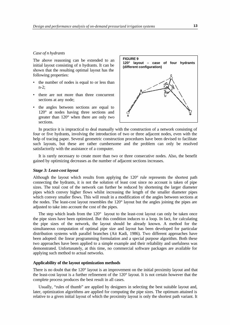
A different configuration of the four hydrants such as the one shown in Figure 9, can lead toa layout involving the creation of only one node since the angle ABM is greater than 120°.

FIGURE 8120° layout – case of four hydrants

Design and performance analysis of on-demand pressurized irrigation systems 13

Case of n hydrants

The above reasoning can be extended to aninitial layout consisting of n hydrants. It can beshown that the resulting optimal layout has thefollowing properties:

• the number of nodes is equal to or less thann-2;

• there are not more than three concurrentsections at any node;

• the angles between sections are equal to120° at nodes having three sections andgreater than 120° when there are only twosections.

In practice it is impractical to deal manually with the construction of a network consisting offour or five hydrants, involving the introduction of two or three adjacent nodes, even with thehelp of tracing paper. Several geometric construction procedures have been devised to facilitatesuch layouts, but these are rather cumbersome and the problem can only be resolvedsatisfactorily with the assistance of a computer.

It is rarely necessary to create more than two or three consecutive nodes. Also, the benefitgained by optimizing decreases as the number of adjacent sections increases.

Stage 3: Least-cost layout

Although the layout which results from applying the 120° rule represents the shortest pathconnecting the hydrants, it is not the solution of least cost since no account is taken of pipesizes. The total cost of the network can further be reduced by shortening the larger diameterpipes which convey higher flows whilst increasing the length of the smaller diameter pipeswhich convey smaller flows. This will result in a modification of the angles between sections atthe nodes. The least-cost layout resembles the 120° layout but the angles joining the pipes areadjusted to take into account the cost of the pipes.

The step which leads from the 120° layout to the least-cost layout can only be taken oncethe pipe sizes have been optimized. But this condition induces to a loop. In fact, for calculatingthe pipe sizes of the network, the layout should be already known. A method for thesimultaneous computation of optimal pipe size and layout has been developed for particulardistribution systems with parallel branches (Ait Kadi, 1986). Two different approaches havebeen adopted: the linear programming formulation and a special purpose algorithm. Both thesetwo approaches have been applied to a simple example and their reliability and usefulness wasdemonstrated. Unfortunately, at this time, no commercial software packages are available forapplying such method to actual networks.

Applicability of the layout optimization methods

There is no doubt that the 120° layout is an improvement on the initial proximity layout and thatthe least-cost layout is a further refinement of the 120° layout. It is not certain however that thecomplete process produces the best result in all cases.

Usually, “rules of thumb” are applied by designers in selecting the best suitable layout and,later, optimization algorithms are applied for computing the pipe sizes. The optimum attained isrelative to a given initial layout of which the proximity layout is only the shortest path variant. It

FIGURE 9120° layout – case of four hydrants(different configuration)

M

Network layout14

could be that a more economic solution is possible by starting with a different initial layout,differing from that which results from proximity considerations, but which takes into accounthydraulic constraints.

In practice, by programming the methods described above for computer treatment, severalinitial layouts of the network can be tested. The first of these should be the proximity layout.The others can be defined empirically by the designer, on the basis of the information available(elevation of the hydrants and distance from the source) which enables potentially problematichydrants to be identified. By a series of iterations it is possible to define a "good" solution, if notthe theoretical optimum. Furthermore, it should be noted that the above estimates are based onthe cost of engineering works only. They do not include the purchase of land, right-of-wayand/or compensation for damage to crops which might occur during construction, all of whichwould affect and increase the cost of the network and might induce to modify the optimallayout.