Forecasting triads:the negative feedback problem

Problem presented by

Stephen Custance-Baker

British Energy

Problem statement

A “Triad” is one of the three half-hour periods in the winter that havethe highest national electricity demand. The charges levied on commercialusers of electricity, for the whole of the winter, depend strongly on theirconsumption during Triad periods. In order to help its customers reducethese costs, British Energy (in common with other large electricity suppliers)attempts to forecast when Triads will occur and warn customers, who canthen reduce their consumption during these periods. However, the very actof warning customers reduces the overall consumption and this may preventa putative Triad from actually occurring. The Study Group was asked toconsider whether this “negative feedback” problem could be prevented.

Study Group contributors

Joyce Aitchison (JMA Numerics)John Billingham (University of Nottingham)John Byatt-Smith (University of Edinburgh)Liam Clarke (London School of Economics)

Jeff Dewynne (University of Oxford)Kim Evans (University of Nottingham)

Vera Hazelwood (Smith Institute)Sam Howison (University of Oxford)

Robert Hunt (University of Cambridge)

Report prepared by

Robert Hunt (University of Cambridge)Liam Clarke (London School of Economics)John Byatt-Smith (University of Edinburgh)John Billingham (University of Nottingham)

D-1

1 Introduction

At the end of the winter season (November 1st to February 28th), National Grid identifiesthe three half-hour periods of highest consumption of electricity, subject to a separationof at least 10 calendar days. These three periods are called Triads. Thus, the half-hourin which national demand was highest is the first Triad; the second highest half-hour,excluding a period of 21 days centred on the first Triad, is the second Triad; and thethird highest half-hour, excluding two periods of 21 days centred on the first and secondTriads, is the third Triad. Historically, Triads always occur on Mondays to Thursdaysbetween 16:30 and 18:00 hours, and not close to Christmas (which is a period of relativelylow consumption). Figure 1 shows the typical pattern over a winter.

Figure 1: National electricity consumption figures from the winter of 03/04. Diamondsindicate daily levels; squares indicate dates on which British Energy issued Triad warnings;and circles indicate those dates on which a Triad was, at the end of the winter, declared tohave occurred.

British Energy supplies electricity to large industrial and commercial customers. Chargesare based on the Transmission Network Use of System (TNUoS) Charges which are leviedby National Grid and passed through to British Energy’s customers. TNUoS includesa substantial surcharge based on each customer’s usage during the Triad periods: thehigher a customer’s usage during Triads, the higher their overall electricity supply costs.

British Energy, in common with other large commercial electricity suppliers, aims toreduce National Grid charges for some of its customers by issuing a “Triad warning” ondays when it seems possible that a Triad might later be found to have occurred. Industrialcustomers are often encouraged by their contract with British Energy to reduce theirconsumption on those warning days. British Energy are restricted by the contract toissuing a limited number of calls over the entire winter period, anything up to 23.

D-2

A customer who receives a Triad warning may, or may not, take action (e.g. shuttingdown their factory early that day). Some – but not all – customers are contractuallyrequired to inform British Energy whether or not they are reducing their consumption.Therefore British Energy cannot be sure by how much overall consumption will drop ifa warning is issued. Furthermore, the national consumption is also affected by suppliersother than British Energy who may also have issued a Triad warning.

It is thought that this system may suffer from “negative feedback”. That is, on aday that is likely to include a Triad period because it has high predicted consumption,many suppliers will issue warnings, resulting in many customers reducing their actualconsumption, ensuring that the total national demand is actually much lower thanpredicted: sufficiently low, in fact, that no Triad occurs, and no warning was actuallynecessary. It is expensive for customers to take action when it is not actually required.

British Energy currently uses the deterministic half-hourly consumption forecast issuedby National Grid and the recent and forecast temperatures at hourly intervals at 7locations around the country to decide on a daily basis whether to issue a Triad warning.The decision-making tool, called TriFoS, does not currently take into account the possibleproblem of negative feedback.

The Study Group was asked to consider ways of compensating for negative feedback. Thenext section confirms that feedback is a statistically significant phenomenon. Sections 3and 4 then use the so-called ‘Full-Information Secretary Problem’ to motivate thederivation of possible triad-calling strategies. Section 5 examines the possibilities forissuing triad warnings from analysing historical data.

2 Detecting feedback

It is understood that a Triad warning issued by British Energy will reduce consumptionby around 200 MW, whilst a warning issued by all suppliers (including British Energy)will reduce consumption on the order of 1200 MW.

An important step was to try to quantify the impact of negative feedback in Triadforecasting. We expect that the issuing of high-consumption warnings affects thebehaviour of British Energy’s commercial customers, encouraging them to reduce theirconsumption. In addition, we expect other supply companies to issue their ownindependent warnings or to react to British Energy’s. To investigate this phenomenonwe look at the forecast errors in National Grid’s consumption forecast on those dayswhen British Energy issued Triad warnings, and compare them to days when warningswere not issued. It is assumed that National Grid’s own consumption forecasts do nottake into account the effects of Triad warnings, in which case, we expect the forecasterror to be larger on those days when warnings are issued.

We divide the days into 4 categories (which are not mutually exclusive), as follows.

• No Warning: days where no Triad warning was made by TriFoS;

D-3

• Low: days where Triad warnings were made and were deemed low probability byTriFoS;

• High: days where Triad warnings were made and were deemed high probability byTriFoS;

• All: days where Triad warnings were made regardless of probability.

Table 1 shows the mean and standard deviation of the consumption forecast error forthese 4 categories. We see that in each case shown here, the mean forecast errors fordays when warnings were issued (All) are larger than on those days when No Warningwas issued. In addition, the mean forecast error for warning days with Low probabilityis, in general, larger than for those warning days with High probability. Whilst theseobservations are encouraging regarding the detection of feedback a more rigorous test isrequired in order to confirm our suspicions.

No Warning Low High AllPeriod N n μ σ n μ σ n μ σ n μ σ01–02 109 90 702 661 12 1084 801 7 989 478 19 1049 68502–03 101 78 759 1162 10 1152 563 13 753 454 23 926 53203–04 94 76 562 503 10 1250 582 8 1091 378 18 1179 49504–05 106 88 471 522 15 875 665 3 778 584 18 858 63705–06 85 62 914 711 15 1055 449 8 1391 839 23 1172 61501–06 495 394 668 757 62 1064 613 39 997 578 101 1038 598

Table 1: Summary of consumption forecast errors showing the period 2001–2006 (in years)and the number of data points. The data is subdivided into No Warning days, Low Triad-probability days, High Triad-probability days, and All Triad days (combining low and highprobability days). The total number of points N , the number of data points of each type n,the mean μ and standard deviation σ of the forecast errors are presented.

Table 2 shows the P -values from a Student t-test on the difference of the means betweenNo Warning and each of Low, High and All. The null hypothesis is that there is nodifference in mean forecast error. This is tested against the alternative hypothesis thatthe mean error is larger for Low, High and All than for No Warning. The test is doneassuming unequal variances in the samples. The values given are the probabilities ofobserving the given result, or one more extreme, by chance if the null hypothesis is true.Small values of P cast doubt on the validity of the null hypothesis.

The test shows clearly that, taking the data over all years, we can reject the nullhypothesis that the mean forecast errors are the same. Therefore, there is clear evidencethat Triad warnings do affect the measured consumption, and negative feedback is a realeffect.

The TriFoS system used by British Energy performs very well, capturing almost all Triadsin the given number of warnings. Indeed, the current maximum number of warnings(23) seems a little generous: in all the years for which TriFoS has been in operation, aconsiderably smaller number would have been sufficient.

D-4

P -valuePeriod Low High All01–02 0.069 0.089 0.02702–03 0.046 0.514 0.16703–04 0.002 0.002 0.00004–05 0.020 0.230 0.01205–06 0.171 0.080 0.05301–06 0.000 0.001 0.000

Table 2: P -values from one-sided t-test on consumption forecast error. The values providedare the probabilities of the corresponding t-statistic.

3 Approaches based on the Secretary Problem

In the Full-Information Secretary Problem (or FISP), one imagines being presented witha sequence of n values, which are drawn independently from some known probabilitydistribution.1 One selects (or ‘calls’) r of the n values, in an attempt to include amongthe selection the M largest values (assuming always that r ≥ M). However, each valuemay be selected only when it is presented, i.e. without knowledge of the values yet tocome, and without going back to any values that have been previously passed over. Theobjective is to devise a strategy that maximises the probability of including the M largestvalues among the r selections. The problem is known for short as the ‘(r, M) FISP’.

The similarity with the calling of Triads should be clear, with the data values beingestimates of daily peak power consumption. However, the Triad-calling problem has twoimportant additional features, namely that energy consumption data is:

(1) Correlated. The best way of predicting the weather today is to guess that it willbe the same as yesterday. Similarly, electricity consumption on a given day is notindependent of energy consumption on the previous day.

(2) Subject to negative feedback. If British Energy call a Triad, many of their customerswill reduce their consumption, as will commercial customers of other electricitysuppliers who provide the same service, thereby reducing the consumption belowthat predicted.

In order to investigate the effects of these two complications, we will study the FISPwith correlation and feedback. We will not, in this report, attempt to include the effectof the ten-day window or to add any uncertainty into the prediction, but these pointsare discussed further in section 6.

Appendix A reviews the optimal strategy for the (1, 1) FISP, as discussed by Gilbertand Mosteller [2], which takes the following form. Suppose that the n data values

1The term ‘full information’ refers to the fact that the underlying distribution of data values isknown.

D-5

0 10 20 30 400.5

0.6

0.7

0.8

0.9

1

i

deci

sion

num

ber,

bi

computedasymptotic for i >> 1

Figure 2: The decision numbers for the Full-Information Secretary Problem with draws froma uniform distribution, and their asymptotic approximation for i � 1.

are y1, y2, . . . , yn. Then the best strategy involves an increasing sequence of decisionnumbers {bi}, which does not depend on n. The ith data point should be called if

yi > bn+1−i and yi = max(yj, j ≤ i) . (1)

In other words, a value is called if it is both the largest value seen so far and largerthan the decision number bj, where j is the number of values yet to come (including thecurrent value). Note that b1 = 0, since we always call the final data point if it the largestin the whole set.

The FISP is most easily studied if the data points are drawn from the uniform distributionon [0 1], U(0, 1), and for the (1, 1) FISP we then have (see the appendix)

bk+1 =1

1 + z, where 1 =

k∑j=1

1

j

(kj

)zj. (2)

Note that b2 = 0.5. It is straightforward to compute the higher decision numbersnumerically and asymptotically they increase to 1 according to

bi+1 ∼ 1 − 0.80435

ias i → ∞. (3)

The decision numbers, along with this asymptotic result, are shown in figure 2. Thedecision numbers bi are monotonically increasing with i. In practice, the optimal strategyfor n large is to wait, unless a data point very close to unity appears, but, as the endof the data set approaches and the decision numbers get smaller, the next data point tocome along that is the largest so far should be called. As discussed in [2], the probabilityof calling the maximum correctly using this strategy, P (win), is about 0.61 when n = 10,and 0.58 when n is large.

D-6

10 20 30 40 50 60 70 80 90 100

−2

0

2

i

10 20 30 40 50 60 70 80 90 100

−2

0

2

10 20 30 40 50 60 70 80 90 100

−2

0

2

data pointsmaximumcallb

n+1−i

Figure 3: Examples of the three possibilities in the (1, 1) FISP with n = 100: the maximum iscalled correctly (top figure), the wrong data point is called (middle figure), or the final pointis reached without a call being made (bottom figure).

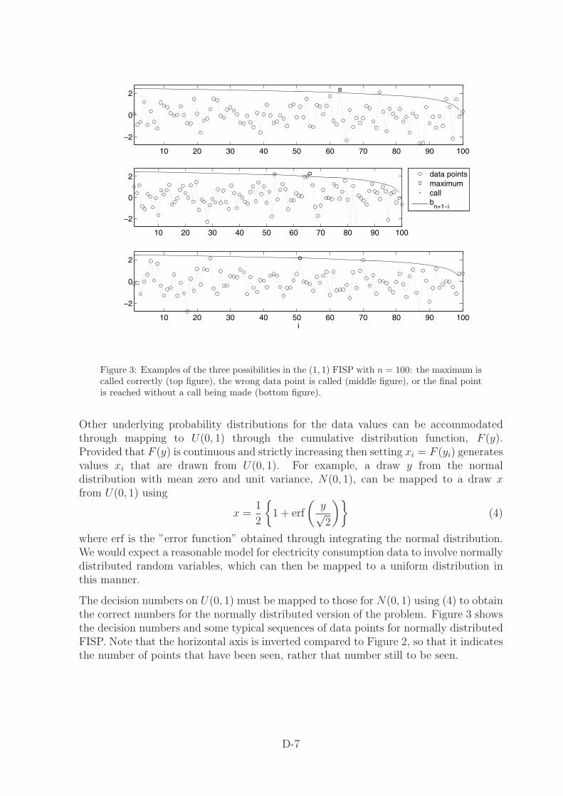
Other underlying probability distributions for the data values can be accommodatedthrough mapping to U(0, 1) through the cumulative distribution function, F (y).Provided that F (y) is continuous and strictly increasing then setting xi = F (yi) generatesvalues xi that are drawn from U(0, 1). For example, a draw y from the normaldistribution with mean zero and unit variance, N(0, 1), can be mapped to a draw xfrom U(0, 1) using

x =1

2

{1 + erf

(y√2

)}(4)

where erf is the ”error function” obtained through integrating the normal distribution.We would expect a reasonable model for electricity consumption data to involve normallydistributed random variables, which can then be mapped to a uniform distribution inthis manner.

The decision numbers on U(0, 1) must be mapped to those for N(0, 1) using (4) to obtainthe correct numbers for the normally distributed version of the problem. Figure 3 showsthe decision numbers and some typical sequences of data points for normally distributedFISP. Note that the horizontal axis is inverted compared to Figure 2, so that it indicatesthe number of points that have been seen, rather that number still to be seen.

D-7

3.1 Framework for incorporating correlation and feedback

In order to model electricity consumption data, we wish to extend the FISP, withnormally distributed data, to take account of correlation and negative feedback. Themodel we use assumes a sequence of n data points of the form

yi+1 = (1 − α) yi + N(0, 1), i = 1, 2, . . . , n − 1, (5)

with y1 = N(0, 1). This means that the series is correlated for O(1/α) data points.With α = 1, this is just the previous case of an uncorrelated draw from N(0, 1), andwith α = 0 it is a random walk. We will study the correlated, (r, M) FISP based on(5). The Triad prediction problem is closely related to this problem with M = 3 (andr = 23). In addition, we will assume that, when a call is made, negative feedback reducesyi to yi − f , with f ≥ 0. We seek the optimal strategy as a function of α, f , r and M .

The random walk without feedback, corresponding to α = 0 and f = 0, was studiedin [3], and we discuss this case in section 3.2. We then extend the analysis to findanalytically the optimal strategy for the (1, 1) uncorrelated FISP with feedback, andan almost optimal strategy for the (r, 1) uncorrelated FISP with no feedback. For thegeneral problem, we determine strategies using Monte Carlo simulation, in Section 4.

3.2 Optimal strategy for the (1, 1) FISP with a random walk

The secretary problem for a random walk, (corresponding to (r, M, α, f) = (1, 1, 0, 0) inthe general framework) was studied in [3], where it was shown that the optimal strategy isto observe the first k data points, and then pick the next data point that is larger than allthe previous points. This is similar to the standard, zero information secretary problem,see [2], where the optimal strategy is the same, and k ∼ n/e as n → ∞. However, forthe random walk, this strategy is optimal for all k. The proof involves rearrangements ofthe sequence of data points, and is not given here. In particular, choosing the first datapoint, and choosing the final data point are both optimal strategies. It is also shown in[3] that the probability of winning using any of these strategies is asymptotic to 1/

√πn

for n large. Finally, we note that, as long as2 b1 = −∞, so that the final data point ischosen if it is a maximum, any sequence of decision numbers bi, possibly including ±∞,gives an optimal strategy.

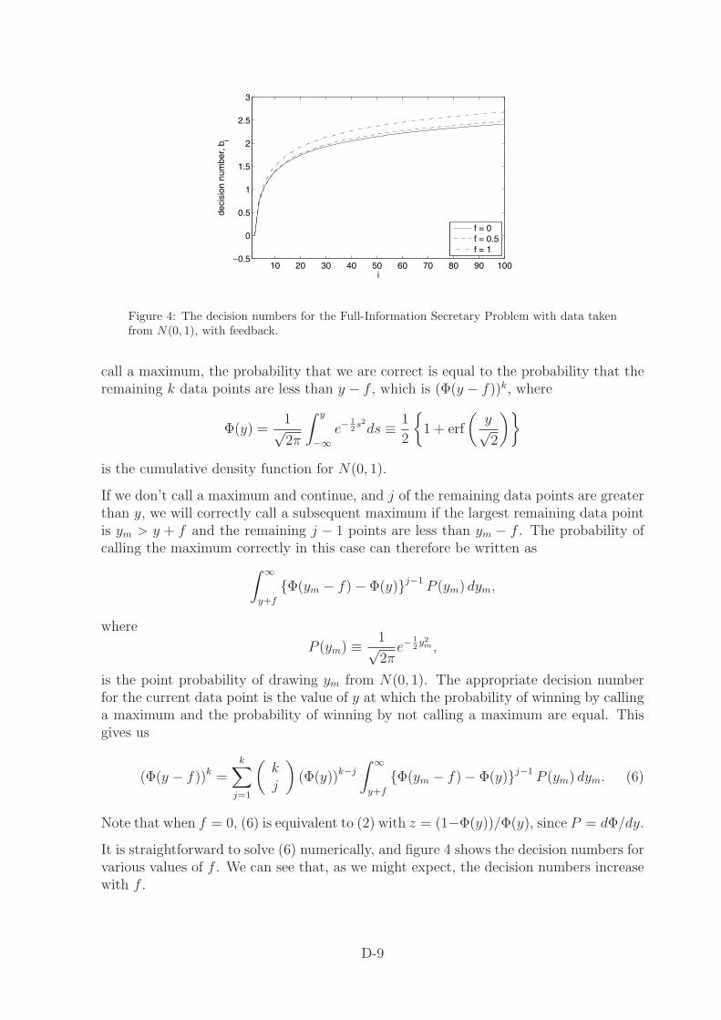
3.3 Optimal strategy for the (1, 1) FISP with feedback

This case has α = 1 and f > 0. We can adapt the method used by Gilbert and Mosteller,[2], described in appendix A, to incorporate feedback. Consider the position when thecurrent data point, chosen from N(0, 1), is y, we have yet to call a maximum, thereare k data points still to come, and y − f is the largest value to appear so far. If we

2Recall that zero in U(0, 1) maps to −∞ in N(0, 1).

D-8

10 20 30 40 50 60 70 80 90 100−0.5

0

0.5

1

1.5

2

2.5

3

i

deci

sion

num

ber,

bi

f = 0f = 0.5f = 1

Figure 4: The decision numbers for the Full-Information Secretary Problem with data takenfrom N(0, 1), with feedback.

call a maximum, the probability that we are correct is equal to the probability that theremaining k data points are less than y − f , which is (Φ(y − f))k, where

Φ(y) =1√2π

∫ y

−∞e−

12s2

ds ≡ 1

2

{1 + erf

(y√2

)}

is the cumulative density function for N(0, 1).

If we don’t call a maximum and continue, and j of the remaining data points are greaterthan y, we will correctly call a subsequent maximum if the largest remaining data pointis ym > y + f and the remaining j − 1 points are less than ym − f . The probability ofcalling the maximum correctly in this case can therefore be written as∫ ∞

y+f

{Φ(ym − f) − Φ(y)}j−1 P (ym) dym,

where

P (ym) ≡ 1√2π

e−12y2

m ,

is the point probability of drawing ym from N(0, 1). The appropriate decision numberfor the current data point is the value of y at which the probability of winning by callinga maximum and the probability of winning by not calling a maximum are equal. Thisgives us

(Φ(y − f))k =k∑

j=1

(kj

)(Φ(y))k−j

∫ ∞

y+f

{Φ(ym − f) − Φ(y)}j−1 P (ym) dym. (6)

Note that when f = 0, (6) is equivalent to (2) with z = (1−Φ(y))/Φ(y), since P = dΦ/dy.

It is straightforward to solve (6) numerically, and figure 4 shows the decision numbers forvarious values of f . We can see that, as we might expect, the decision numbers increasewith f .

D-9

0 0.5 1 1.5 20

0.1

0.2

0.3

0.4

0.5

0.6

0.7

f

P(w

in)

n = 50n = 100n = 250

Figure 5: The probability of winning in the Full-Information Secretary Problem with feedbackf , for various n.

We have not attempted to calculate the probability of winning analytically, but haveestimated it using Monte Carlo simulation with 105 trials. Figure 5 shows the probabilityof winning as a function of f . Clearly, feedback has a significant effect on the probabilityof calling the maximum, which decreases monotonically with f . In addition, althoughP (win) asymptotes to a constant value as n → ∞ when f = 0, this does not appear tobe the case for f > 0, and we conjecture that P (win) → 0 as n → ∞.

3.4 An almost-optimal strategy for the (r, 1) FISP

We return now to the case with no correlation and no feedback, but allow several callsto be made. We can extend the method used by Gilbert and Mosteller, [2], describedin appendix A, which works when r = 1, to find a strategy for uncorrelated FISP withr > 1. Once we have a strategy for the cases r < S, then we have a strategy for the caser = S once a single call has been made. In particular, we look for a strategy involvingdecision numbers bR

i , for i = 1, 2, . . . , n and R = 1, 2, . . . , r, such that a call should bemade if, with R calls remaining in hand, yi > bR

n+1−i and yi = max(yj, j ≤ i). It is easiesthere to work with data points taken from the uniform distribution, U(0, 1), transformingthe results as required to other distributions.

Consider the position when the current data point, x, is the largest so far, we have Rcalls available, and there are k data points still to come. If we call a maximum, theprobability that either x is the maximum or we will still be able to call the maximumwith one of our R − 1 remaining calls, is composed of two parts, say P1 + P2. Theseare, firstly, the probability that no more than R − 1 of the remaining k data points aregreater than x,

P1 =R−1∑j=0

(kj

)xk−j (1 − x)j ,

and secondly, the probability P2 that, if there are j ≥ R data points remaining that arebigger than x, then they are ordered so that the R − 1 remaining calls suffice to find

D-10

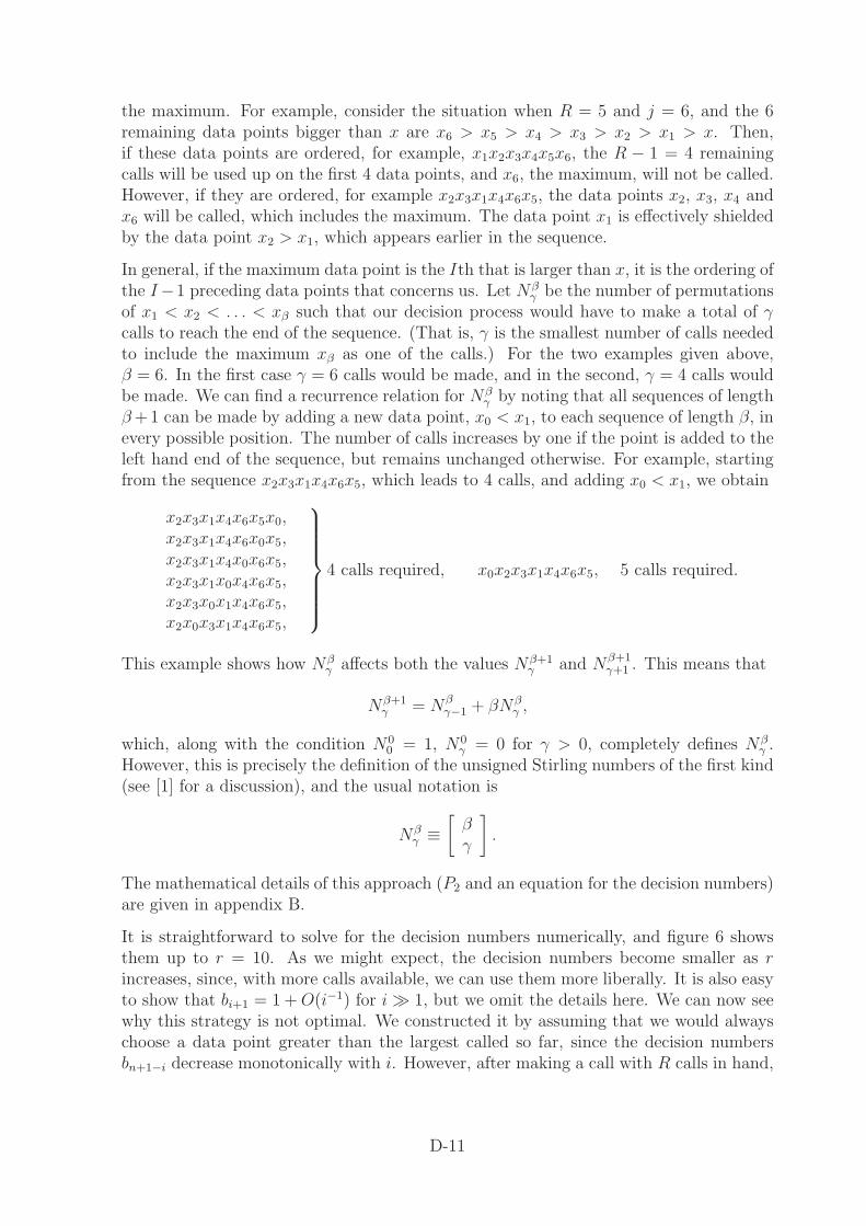
the maximum. For example, consider the situation when R = 5 and j = 6, and the 6remaining data points bigger than x are x6 > x5 > x4 > x3 > x2 > x1 > x. Then,if these data points are ordered, for example, x1x2x3x4x5x6, the R − 1 = 4 remainingcalls will be used up on the first 4 data points, and x6, the maximum, will not be called.However, if they are ordered, for example x2x3x1x4x6x5, the data points x2, x3, x4 andx6 will be called, which includes the maximum. The data point x1 is effectively shieldedby the data point x2 > x1, which appears earlier in the sequence.

In general, if the maximum data point is the Ith that is larger than x, it is the ordering ofthe I−1 preceding data points that concerns us. Let Nβ

γ be the number of permutationsof x1 < x2 < . . . < xβ such that our decision process would have to make a total of γcalls to reach the end of the sequence. (That is, γ is the smallest number of calls neededto include the maximum xβ as one of the calls.) For the two examples given above,β = 6. In the first case γ = 6 calls would be made, and in the second, γ = 4 calls wouldbe made. We can find a recurrence relation for Nβ

γ by noting that all sequences of lengthβ +1 can be made by adding a new data point, x0 < x1, to each sequence of length β, inevery possible position. The number of calls increases by one if the point is added to theleft hand end of the sequence, but remains unchanged otherwise. For example, startingfrom the sequence x2x3x1x4x6x5, which leads to 4 calls, and adding x0 < x1, we obtain

x2x3x1x4x6x5x0,x2x3x1x4x6x0x5,x2x3x1x4x0x6x5,x2x3x1x0x4x6x5,x2x3x0x1x4x6x5,x2x0x3x1x4x6x5,

⎫⎪⎪⎪⎪⎪⎪⎬⎪⎪⎪⎪⎪⎪⎭

4 calls required, x0x2x3x1x4x6x5, 5 calls required.

This example shows how Nβγ affects both the values Nβ+1

γ and Nβ+1γ+1 . This means that

Nβ+1γ = Nβ

γ−1 + βNβγ ,

which, along with the condition N00 = 1, N0

γ = 0 for γ > 0, completely defines Nβγ .

However, this is precisely the definition of the unsigned Stirling numbers of the first kind(see [1] for a discussion), and the usual notation is

Nβγ ≡

[βγ

].

The mathematical details of this approach (P2 and an equation for the decision numbers)are given in appendix B.

It is straightforward to solve for the decision numbers numerically, and figure 6 showsthem up to r = 10. As we might expect, the decision numbers become smaller as rincreases, since, with more calls available, we can use them more liberally. It is also easyto show that bi+1 = 1 + O(i−1) for i � 1, but we omit the details here. We can now seewhy this strategy is not optimal. We constructed it by assuming that we would alwayschoose a data point greater than the largest called so far, since the decision numbersbn+1−i decrease monotonically with i. However, after making a call with R calls in hand,

D-11

20 40 60 80 1000

0.2

0.4

0.6

0.8

1

i

deci

sion

num

ber,

br i

increasing R

Figure 6: The decision numbers for the Full-Information Secretary Problem with draws froma uniform distribution and r calls, for r up to 10.

we switch to the decision numbers appropriate for R − 1 calls in hand, which meansthat the decision number increases discontinuously after each call. There is thereforethe possibility of a data point arriving that is bigger than the largest point called so far,but smaller than the appropriate decision number, contradicting the assumptions thatunderlie the construction. We shall however see in the next section that our strategy isclose to optimal.

Finally, figure 7 shows the probability of calling the maximum as a function of r whenn = 100. The probability of calling the maximum increases with r, and is greater than0.99 when r = 5. Also shown is the probability of winning using the simpler strategysuggested by Gilbert and Mosteller, [2], which uses a sequence of decision numbers thatdepends upon r, but is independent the number of calls made. As we would expect, thestrategy derived here gives a slightly higher probability of calling the maximum.

4 Optimal strategies by Monte Carlo simulation

In order to investigate the cases for which we cannot derive an optimal strategyanalytically, we will use Monte Carlo simulation. Before outlining the procedure, weneed to take note of two features of the problem.

Optimal strategy with feedback and more than one call (f > 0, r > 1)

With just one call available, r = 1, we showed in section 3.3 that we can derive theoptimal strategy. In particular, it is clear that we should not make our call until thecurrent data point exceeds by more than f the largest data point to appear so far, sincefeedback will otherwise reduce it too far for it to remain a maximum. When r > 1, the

D-12

1 2 3 4 5 60.4

0.6

0.8

1

r

P(w

in)

new strategyGilbert and Mosteller strategy

1 2 3 4 5 610

−3

10−2

10−1

100

1−P

(win

)

r

Figure 7: Probability of calling the maximum with r calls, from Monte Carlo simulation with105 trials and n = 100. Also shown is the strategy due to Gilbert and Mosteller [2].

situation is not so clear. If we use this approach at every data point, we may discard asequence of increasing data points, and push ever higher the threshold above which wewill actually call. An alternative strategy is, if we have more than one call still available,to make a call whenever the current data point exceeds the greatest value not called.Although we know that we will not necessarily call a maximum, we will reduce the valueof the called point by f , so that the threshold does not increase. We can then, with oneof our remaining calls, hope to call a data point that is large enough that, even withthe effect of feedback, it is actually a maximum. This is the strategy that we adoptbelow. However, we might envisage cases where the current data point only exceedsthe previous maximum by a small amount, in which case we would not want to wastea call on it. This suggests that an optimal strategy involves an additional sequence ofnumbers, {δR

i (f)}, such that with i data points and R possible calls remaining, we callif the current data point exceeds the previous maximum by more than δR

i . We mightexpect that δR

i 1 when R � 1 and that δ1i = f . We have yet to investigate this more

sophisticated strategy further. In effect, we assume that δ1i = f and δR

i = 0 for R > 1.

Optimal strategy for calling more than one maximum (M > 1)

When the M > 1 largest data points are to be called, the optimal strategy is verydifficult to calculate, since the decision number depends not only on how many datapoints remain, but also the relative sizes of the previous data points and, once a callhas been made, the size of the data points called. As an example, we can study the

D-13

(2, 2) FISP. Consider the situation when we have yet to make a call. If we try to usethe method described earlier, we must calculate the probability of calling the two largestdata points, firstly if we call the current data point, and secondly if we do not call thecurrent data point. If we make a call, the probability of winning is the probability that,of the remaining k data points, just one is bigger than the second highest data pointseen so far, which is not the current data point, but the previous highest data point. Inother words, the optimal strategy must depend upon not only the current data point,but also the previous highest data point. The decision numbers are therefore functionsnot just of i and R, but also of, in this example, the previous highest data point, and ingeneral, the previous M − 1 highest data points. It may be possible to sort this out inprinciple, and even in practice, but we have not attempted to do so here. Instead, welook for decision numbers b

(R,M)i that are dependent only upon i, R and M , as described

below.

4.1 Monte Carlo simulations with M = 1

4.1.1 Numerical method

In principle, when successive data points are correlated, we could use the methodsdescribed in section 3 to calculate the decision numbers. However, in practice, it is notpossible to determine analytically the probabilities of winning by calling or not callinga given data point, because of the complicated conditional probabilities that need to becalculated. Instead, we calculate the decision numbers numerically using Monte Carlosimulation. Specifically, if we know the decision numbers br

i for 1 ≤ i < j and bRi for

1 ≤ i ≤ n and 1 ≤ R < r, we can calculate brj numerically. Using n = j, we can calculate

the probabilities of winning by calling the first data point, Pc, and by not calling it, Pnc,using Monte Carlo simulation, evolving yi using (5), including the effect of feedback ifnecessary, since we know the decision numbers for the subsequent j − 1 data points. Inthis manner we can compute G(y1) ≡ Pc − Pnc. By construction, bj is the solution ofG(y1) = 0. Since we compute G by Monte Carlo simulation, we cannot rely on it beingsmooth, so we use a bisection method to find the root. This works well in practice untilthe probabilities Pc and Pnc both become either small or close to unity. In these cases,the function G eventually becomes too noisy to work with. In the results that follow,we have used Monte Carlo simulation with 105 trials to estimate G. Finally, note that,since we know that bR

i = −∞ for 1 ≤ i ≤ R (the final R data points should be calledif they are maxima), we have a place to start our calculation, and therefore a practicalalgorithm for calculating the decision numbers.

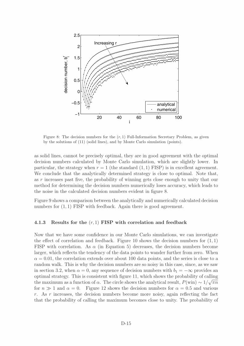
4.1.2 Validation for the (r, 1) FISP and (1, 1) FISP with feedback

We begin by validating our numerical method against the analytical results that weobtained earlier. Figure 8 shows the decision numbers for the (r, 1) FISP calculatedboth numerically, by Monte Carlo simulation, and analytically using the results ofsection 3.4. Although, as we discussed above, the analytical decision numbers, shown

D-14

20 40 60 80 100−1

−0.5

0

0.5

1

1.5

2

2.5

i

deci

sion

num

ber,

br i

analyticalnumerical

Increasing r

Figure 8: The decision numbers for the (r, 1) Full-Information Secretary Problem, as givenby the solutions of (11) (solid lines), and by Monte Carlo simulation (points).

as solid lines, cannot be precisely optimal, they are in good agreement with the optimaldecision numbers calculated by Monte Carlo simulation, which are slightly lower. Inparticular, the strategy when r = 1 (the standard (1, 1) FISP) is in excellent agreement.We conclude that the analytically determined strategy is close to optimal. Note that,as r increases past five, the probability of winning gets close enough to unity that ourmethod for determining the decision numbers numerically loses accuracy, which leads tothe noise in the calculated decision numbers evident in figure 8.

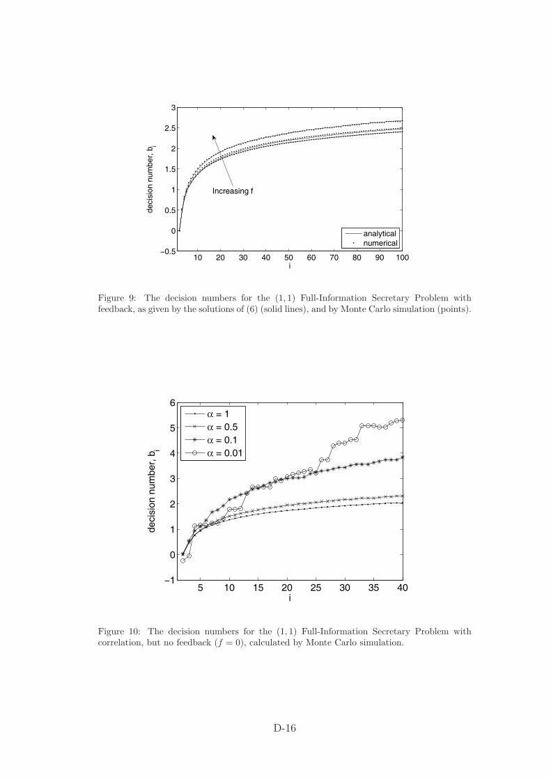
Figure 9 shows a comparison between the analytically and numerically calculated decisionnumbers for (1, 1) FISP with feedback. Again there is good agreement.

4.1.3 Results for the (r, 1) FISP with correlation and feedback

Now that we have some confidence in our Monte Carlo simulations, we can investigatethe effect of correlation and feedback. Figure 10 shows the decision numbers for (1, 1)FISP with correlation. As α (in Equation 5) decreases, the decision numbers becomelarger, which reflects the tendency of the data points to wander further from zero. Whenα = 0.01, the correlation extends over about 100 data points, and the series is close to arandom walk. This is why the decision numbers are so noisy in this case, since, as we sawin section 3.2, when α = 0, any sequence of decision numbers with b1 = −∞ provides anoptimal strategy. This is consistent with figure 11, which shows the probability of callingthe maximum as a function of α. The circle shows the analytical result, P (win) ∼ 1/

√πn

for n � 1 and α = 0. Figure 12 shows the decision numbers for α = 0.5 and variousr. As r increases, the decision numbers become more noisy, again reflecting the factthat the probability of calling the maximum becomes close to unity. The probability of

D-15

10 20 30 40 50 60 70 80 90 100−0.5

0

0.5

1

1.5

2

2.5

3

i

deci

sion

num

ber,

bi

analyticalnumerical

Increasing f

Figure 9: The decision numbers for the (1, 1) Full-Information Secretary Problem withfeedback, as given by the solutions of (6) (solid lines), and by Monte Carlo simulation (points).

5 10 15 20 25 30 35 40−1

0

1

2

3

4

5

6

i

deci

sion

num

ber,

bi

α = 1α = 0.5α = 0.1α = 0.01

Figure 10: The decision numbers for the (1, 1) Full-Information Secretary Problem withcorrelation, but no feedback (f = 0), calculated by Monte Carlo simulation.

D-16

0 0.2 0.4 0.6 0.8 10

0.1

0.2

0.3

0.4

0.5

0.6

0.7

α

P(w

in)

numericalanalytical for α = 0, a random walk

Figure 11: The probability of calling the maximum for the (1, 1) Full-Information SecretaryProblem with correlation, but no feedback (f = 0), and n = 100 data points, calculated byMonte Carlo simulation.

calling the maximum is shown in figure 13 for various values of r as a function of α. Itis clear that, even with correlation, the probability of winning rapidly approaches unityas r increases, unless α is close to 1/n, which is equal to 0.01 in this case.

Finally, we present some results with f = 0.5. Figure 14 shows the decision numberswhen f = 0.5 and the data points are uncorrelated (α = 1). One striking feature of thisplot is the gap between the decision numbers for r = 1 and those for r = 2, which issignificantly larger than the gaps between the remaining sets of decision numbers. Thisis probably because the optimal strategy involves the additional sequence {δr

i }, describedearlier. In our simulations, we call a maximum whenever a new largest point arrives,even if we know that feedback will reduce it below the threshold, until we have just onecall remaining, when we have to exercise more caution. The probability of calling themaximum using these decision numbers is shown in figure 15, and is significantly smallerfor a given r than when there is no feedback (see figure 13). Figures 16 and 17 showthe results when f = 0.5 and α = 0.2. Although the decision numbers are somewhatlarger than those shown in figure 14, the probabilities of calling the maximum shownin figure 17 are not very different from those when there is no correlation, shown infigure 15, which suggests that feedback is the dominant mechanism that determines theprobability of success.

D-17

5 10 15 20 25 30 35 40−1.5

−1

−0.5

0

0.5

1

1.5

2

2.5

i

deci

sion

num

ber,

br i

Increasing r

Figure 12: The decision numbers for the (r, 1) Full-Information Secretary Problem withcorrelation α = 0.5, but no feedback (f = 0), calculated by Monte Carlo simulation.

0 0.2 0.4 0.6 0.8 10

0.2

0.4

0.6

0.8

1

α

P(w

in)

Increasing r

Figure 13: The probability of calling the maximum for the (r, 1) Full-Information SecretaryProblem with correlation, but no feedback (f = 0), and n = 100 data points, calculated byMonte Carlo simulation.

D-18

5 10 15 20 25 30 35 40−1

−0.5

0

0.5

1

1.5

2

2.5

i

deci

sion

num

ber,

br i

Increasing r

Figure 14: The decision numbers for the (r, 1) Full-Information Secretary Problem with nocorrelation (α = 1), and feedback f = 0.5, calculated by Monte Carlo simulation.

2 4 6 8 10 12 140.1

0.2

0.3

0.4

0.5

0.6

0.7

0.8

0.9

r

P(w

in)

Figure 15: The probability of calling the maximum for the (r, 1) Full-Information SecretaryProblem no correlation (α = 1), and feedback f = 0.5, and n = 100 data points, calculatedby Monte Carlo simulation.

D-19

5 10 15 20 25 30 35 40−3

−2

−1

0

1

2

3

4

i

deci

sion

num

ber,

br i

Increasing r

Figure 16: The decision numbers for the (r, 1) full information secretary problem withcorrelation α = 0.2, and feedback f = 0.5, calculated by Monte Carlo simulation.

2 4 6 8 10 12 140.1

0.2

0.3

0.4

0.5

0.6

0.7

0.8

0.9

r

P(w

in)

Figure 17: The probability of calling the maximum for the (r, 1) full information secretaryproblem correlation α = 0.2, and feedback f = 0.5, and n = 100 data points, calculated byMonte Carlo simulation.

D-20

4.2 Monte Carlo simulations with M > 1

As discussed earlier, the optimal strategy in this case depends explicitly on the previousdata points. We will not attempt to unravel this here, but instead propose a simplerstrategy. We will assume that there are sequences of decision numbers, {b(r,m)

i }, with1 ≤ m ≤ M , which govern the selection of the first M calls when m calls remain tobe made. However, once we have called at least M data points, we make another callonly if the current data point is larger than the Mth largest of those already seen. Itseems likely that this strategy is close to optimal since, as we saw above, our analyticallydetermined strategy for the (r, 1) FISP is close to optimal, even though it was constructedon precisely this basis (with at least one call made, call if the current point is the largestso far). We can calculate the decision numbers numerically in the same way as we didfor the case M = 1. However, for these calculations, we used just 104 trials, since thealgorithm required to sort out the position of the current data point relative to thosecalled so far is rather time consuming, so that the accuracy of the following results issomewhat lower than those described above.

4.2.1 Results for the (r, M) FISP

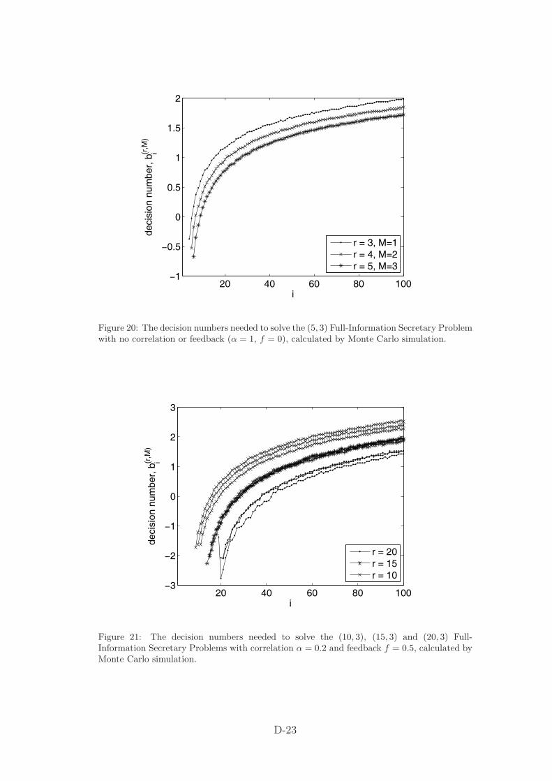
Figure 18 shows the decision numbers when r = M , with neither correlation nor feedback.Note that, for example, the decision numbers for the (3, 3) FISP are given by the thirdlargest set in figure 18, but, once a call has been made, switches to the next largestcurve, which is also appropriate for the (2, 2) FISP, and so on. As we might expect, thedecision numbers decrease with M , since we need to select more points. Figure 19 showsthe associated probabilities of calling all M maxima, which obviously decrease with M ,but perhaps not by as much as one might expect. The decision numbers needed for the(5, 3) FISP are shown in figure 20. We find that the probability of calling all three of thelargest data points is 0.32, 0.60 and 0.79 for r = 3, 4 and 5 respectively, and n = 100.

Results for the (r, M) FISP with correlation and feedback

Since we now have a large parameter space to explore, we will restrict our attention to acase that seems relevant to the triads problem, namely α = 0.2 (correlation over aboutfive data points), f = 0.5 and M = 3, for various values of r. Figure 21 shows the threesets of decision numbers for r = 10, 15 and 20. We can see that, as r gets larger, thesets become closer to each other. This is in line with British Energy’s current practice,where a single threshhold (decision number) is used to decide whether or not to call.Although one of the r = 20 sets is a little different from the other two, this is probablydue to numerical error, since it contains the decision numbers for the (18, 1) FISP, forwhich the probability of calling the maximum is greater than 0.99. Figure 22 shows theprobability of calling the three largest data points as a function of r. This is greater than0.9 when r ≥ 18. Also shown for comparison are the same probabilities when there isno feedback and/or no correlation. Just as we found when M = 1, the effect of feedbackon these probabilities is significantly greater than the effect of correlation. This is anaspect of the problem that could be investigated further.

D-21

20 40 60 80 100−1.5

−1

−0.5

0

0.5

1

1.5

2

2.5

i

deci

sion

num

ber,

b(r

,M)

i

increasing r = M

Figure 18: The decision numbers for the (M,M) Full-Information Secretary Problem with nocorrelation or feedback (α = 1, f = 0), calculated by Monte Carlo simulation.

1 2 3 4 5 6

0.2

0.25

0.3

0.35

0.4

0.45

0.5

0.55

0.6

r=M

P(w

in)

Figure 19: The probability of calling the M largest values for the (M,M) Full-InformationSecretary Problem with no correlation or feedback (α = 1, f = 0), calculated by Monte Carlosimulation for n = 100.

D-22

20 40 60 80 100−1

−0.5

0

0.5

1

1.5

2

i

deci

sion

num

ber,

b(r

,M)

i

r = 3, M=1r = 4, M=2r = 5, M=3

Figure 20: The decision numbers needed to solve the (5, 3) Full-Information Secretary Problemwith no correlation or feedback (α = 1, f = 0), calculated by Monte Carlo simulation.

20 40 60 80 100−3

−2

−1

0

1

2

3

i

deci

sion

num

ber,

b(r

,M)

i

r = 20r = 15r = 10

Figure 21: The decision numbers needed to solve the (10, 3), (15, 3) and (20, 3) Full-Information Secretary Problems with correlation α = 0.2 and feedback f = 0.5, calculated byMonte Carlo simulation.

D-23

0 5 10 15 20 250

0.1

0.2

0.3

0.4

0.5

0.6

0.7

0.8

0.9

1

r

P(w

in)

α = 0.2, f=0α = 0.2, f=0.5α = 1, f=0.5α = 1, f=0

Figure 22: The probability of calling the 3 largest values for the (r,M) Full-InformationSecretary Problem with correlation α = 0.2 and feedback f = 0.5, calculated by Monte Carlosimulation for n = 100. In order to compare the effects of correlation and feedback, the resultsfor α = 1 and/or f = 0 are also shown.

5 Criteria based on analysis of historical data

As previously described, the current algorithm used by British Energy, implementedby TriFoS, is extremely effective. However, in this section we consider alternative oradditional criteria that might be used for deciding whether to issue a Triad warning.Such criteria would involve rewriting the TriFoS algorithm and are therefore unlikely tobe implemented; however, they are interesting in their own right.

Notation:

(1) We define the actual Peak Power consumption on a given day in year n as Ca(i, n)with 1 ≤ i ≤ 120 representing the date and n the year. Here we take n in the range1 ≤ n ≤ 5 corresponding to years 2001/02 to 2005/06 and dates from 1/11/n to28/2/(n + 1). Forecast Peak Power consumption Cf (i, n) is defined similarly.

(2) From Ca(i, n) and Cf (i, n) we define C̃a(i, n) and C̃f (i, n) which are the orderedPeak Power consumptions, with C̃a(1, n) > C̃a(2, n) > · · · > C̃a(120, n).

Notes:

(1) For technical reasons, historical figures are not available on every single day. Thenumber of total Actuals and Forecasts are given in Table 3.

D-24

Year Number of Actuals Number of Forecasts2001/02 60 582002/03 55 522003/04 60 572004/05 64 632005/06 64 64

Table 3: Number of Actual and Forecast Peak Power levels recorded.

(2) In 2005/06 Scotland was included for the first time. In order to compare C̃a(i, 5)with C̃a(i, n), n < 5, we subtract an estimated consumption for Scotland using theestimate Ca(i, 5) − 1

4

∑4n=1 Ca(i, n).

(3) It is important when comparing consumption from year to year to attempt to makesure that we are looking at data collected in the same way. Hence we have onlyused C̃a(i, n) and C̃f (i, n) for i in the range 1 ≤ i ≤ 50.

(4) We assume that TriFoS is able, or can be adapted, to produce a good forecast ofthe actual consumption Ca(i, n) on a given day i, either with or without takinginto account the effects of negative feedback. We also presume that this forecastis better than that given by National Grid. Although actual consumption andthe National Grid forecast are clearly well correlated (with a correlation coefficientof 0.95; see Figure 23), we find that the National Grid forecast minus the actualconsumption, for the year 05/06, has a mean of 881 with a standard deviation of556. Least-squares fit of a straight line gives a slight slope, but is not very differentto the line with height equal to the mean (see again the figure). The higher NationalGrid estimate is partially but not entirely due to negative feedback.

It is clear from this graph that a year-by-year comparison on a given day will havequite a large random element in it.

Aims:

(1) We want to attempt to remove as much as possible of the random element in thefigures, and to do that we compare the ordered forecasts, C̃a(i, n).

(2) We then want to see if we can make a good estimate of when we should issue a Triadwarning, assuming that a good estimate of the actual consumption is available.

(3) The days close to an actual Triad are excluded because of the ten-day rule. Ifwe filter these out then the top three in the amended list are the Triads. The iassociated with the C̃a(i, n) of the Triads form a subsequence relating where theTriads appear in the ordered list. We note here that for the available data all Triaddays have i < 20, as is given in Table 4.

D-25

52000

54000

56000

58000

60000

0 10 20 30 40 50 60

xx

Figure 23: National Grid forecast and actual consumption for 2005/06. The top two curvesare respectively the forecast and the actuals. The lower curve is the difference, with the lowerline representing the axis and the upper line the mean of 881.

Year Triad 1 Triad 2 Triad 32001/02 1 2 172002/03 1 2 142003/04 1 4 112004/05 1 4 142005/06 1 9 12

Table 4: The ordinal i associated with each Triad.

D-26

48000

49000

50000

51000

52000

53000

54000

1 2 3 4 5

Figure 24: Graph joining the points C̃a(i, n) for fixed i and 1 ≤ n ≤ 5, with the Scottishaverage subtracted in the year 2005/06.

Figure 24 is a piecewise continuous graph joining the points C̃a(i, n) for fixed i with1 ≤ n ≤ 5, where the estimated Scottish average of 6991 is subtracted to make datauniform from year to year. The top 40 of these graphs are shown and the circles representthe average of the top 40 for a given year. Suppose we define the signature of each graph,for example (+,−, +,−), as the sign of the piecewise derivative, that is the sign of theslope of the graph between year n and n+1 for a fixed value of i. It is clear that C̃a(1, n)dominates, in that its signature is shared by most of the other graphs as we vary i. Theaverage also has this same signature and thus is a good indicator of the shape of eachgraph for fixed i.

From these observations, the average is not the only feature that determines the topstructure in the ordered list: the signature is also an important feature. In order topredict this structure accurately it is therefore good to use at least two parameters. Forissuing Triad warnings, the objective is to predict the level of consumption C̃a(20, n)from the previous years’ data and any data so far available for the current year to date.The average of C̃a(20, n) still shows a sizable random element from year to year as isseen from the circles in Figure 24 and in Table 5. While the difference shows that theaverage is well approximated by the average of the top 40, as we would expect, there isa larger random yearly element.

We now turn our attention to the best parameters to determine the values of C̃a(i, n)in the ordered list. As we indicated earlier we require two parameters and this suggeststhat we should be looking at a straight line fit.

Figure 25 plots C̃a(i, n), for n fixed and i in the range 1 ≤ i ≤ 40, and the best straightline fit. All 5 years are superimposed: it is not really important to know which year iswhich, it is the distribution of errors that is important. Figure 26 shows the error of the

D-27

Year C̃a(20, n) Average Difference2001/02 49791 49859 −682002/03 50872 51376 −5042003/04 51001 51168 −1672004/05 51572 51616 −442005/06 57868 57995 −127

Table 5: Comparison between C̃a(20, n) and the average of the top 40.

50000

52000

54000

56000

58000

01/2

02/3

03/404/5

05/6

0 10 20 30 40

Figure 25: Graphs joining the points C̃a(i, n) for a fixed n, with the best straight line fit.

D-28

–400

–200

0

200

400

600

800

1000

10 20 30 40

Figure 26: Errors in the straight-line fit of the top 40.

Year C̃a(15, n) Linear C̃a(20, n) Linear C̃a(25, n) Linearfit fit fit

2001/02 50033 50059 49791 49742 49440 494242002/03 51595 51493 50872 50980 50576 504662003/04 51326 51261 51001 51020 50810 507782004/05 51766 51761 51572 51593 51431 514252005/06 58349 58244 57868 57938 57712 57631

Table 6: Comparison between C̃a(i, n) and the linear fit for i = 15, 20 and 25.

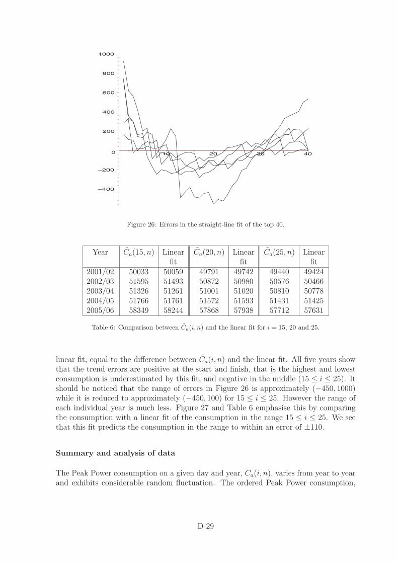
linear fit, equal to the difference between C̃a(i, n) and the linear fit. All five years showthat the trend errors are positive at the start and finish, that is the highest and lowestconsumption is underestimated by this fit, and negative in the middle (15 ≤ i ≤ 25). Itshould be noticed that the range of errors in Figure 26 is approximately (−450, 1000)while it is reduced to approximately (−450, 100) for 15 ≤ i ≤ 25. However the range ofeach individual year is much less. Figure 27 and Table 6 emphasise this by comparingthe consumption with a linear fit of the consumption in the range 15 ≤ i ≤ 25. We seethat this fit predicts the consumption in the range to within an error of ±110.

Summary and analysis of data

The Peak Power consumption on a given day and year, Ca(i, n), varies from year to yearand exhibits considerable random fluctuation. The ordered Peak Power consumption,

D-29

–100

–50

0

50

100

16 18 20 22 24

Figure 27: Errors in a straight-line fit restricted to 15 ≤ i ≤ 25.

C̃a(i, n), shown in Figure 24 displays much less fluctuation from year to year. We alsoshow in Figure 25 that for a fixed year the ordered Peak Power consumption can be wellapproximated by a straight line. However we should remember that Figure 25 also showsthat there is considerable variation of this fit from year to year. The error in the straightline fit of the top forty is shown in Figure 26, while the goodness of fit of the top 15 to 25is shown in Figure 27, which shows that the absolute error is less than 110. We should,of course, point out that while it is easy to fit this straight line “after” the event, that isat the end of the year, it is more difficult to predict this fit at the beginning of the year.However tables 4 and 5 show that if we are able to predict the value of C̃a(20, n) weshould be able to predict, and thereby issue a warning for, all the likely Triad events. Ifwe do issue warnings for all of the top 20 then the problem of negative feedback shouldalmost disappear, because we expect to have caught all the Triads.

Predicting the value of C̃a(20, n)

While predicting the value of C̃a(20, n) is the main aim, we suggest that the best strategyis to predict the linear fit. This requires two parameters, either the mean and the slope,or perhaps better using two points. We suggest that we take C̃a(15, n) and C̃a(25, n).However we should remember that we are not actually trying to predict C̃a(15, n) andC̃a(25, n) but merely the straight line, which will then give not only give an estimate ofC̃a(20, n) but also an estimate of the error in the predicted value. We also note that aquadratic fit requires three points and a cubic four points which would be very difficultto forecast accurately.

We can get some prior estimate from Table 6, taking into account that Scotland is

D-30

included in the consumption figures now. What is then required is to update theseestimates in the light of the consumption figures of early November, before the likelyperiod of the first Triad date, and throughout the year as more data comes in. We havenot attempted to do this. However we should remember that an estimated linear fit willnot have as good error bounds as the actual fit and this should be taken into accountwhen deciding whether to issue a warning. The best suggestion is for this alternativemethod to be used in a trial period running simultaneously with the present TriFoSmethod and comparing the results at the end of the year to see which gives the betterresults.

6 Conclusions and further work

We began the study by conducting an analysis of the errors in National Grid’sconsumption forecasts, which revealed a statistically significant dependence on whetheror not Triads calls had been issued by British Energy. This result confirms that negativefeedback is present in practice. We then went on to consider two broad ways ofapproaching the question of identifying Triads as they occur, based on extensions ofthe Full-Information Secretary Problem, and a direct analysis of historical data.

Methods based on the Full-Information Secretary Problem

We have shown that by studying (r, 3) Full-Information Secretary Problem with feedbackand correlation we can gain some insight into the Triads problem, and that our results,which suggest that about 18 calls are needed to be able to find the three largest datapoints 90% of the time, are in line with the experience of British Energy. Our resultsalso indicate that negative feedback may be a more important issue than the correlatednature of the data. We were also able to derive some new analytical results for the (r, 1)FISP and (1, 1) FISP with feedback.

In order to make these simulations more realistic, we would need to include the effect ofthe ten-day window, and add some uncertainty into the prediction. For example, thisuncertainty could take the form of a value chosen from a normal distribution and addedto each data point after the decision to call or not has been taken. The optimal, or atleast a good, strategy then needs to be more complicated. We would wish to call datapoints whose predicted value is not one of the three largest so far, but is sufficiently largethat uncertainty may make them so.

In addition, we note that the Triad problem has two more subtle aspects in practice.Firstly, the aim should be to maximise the expected number of triads called, not tomaximise the probability of calling all three triads. However, when the probability ofthe latter is close to unity, the expected number of triads called is sure to be close tothree. Secondly, British Energy would like to minimise the number of calls made. Thishas not been addressed here, as we have assumed that a fixed number of calls, r, isavailable. It would be worth looking at the results again to assess the expected number

D-31

of calls, which is likely to be less than r when r is large, but we have not attempted thishere.

Methods based on analysis of historical data

If peak daily consumptions through the winter are placed in decreasing order, then theTriad days always seem to fall within the top 20. Since British Energy has at least 20calls available, calling the top 20 will catch the actual Triads (as above, this line ofthinking does not attempt to minimise the number of calls made). We therefore lookedat ways of predicting the twentieth highest daily consumption and found that, withineach year, a simple linear fit to the ordered daily peak consumptions may be sufficient.Although there is significant variation from year to year, it may be possible to use actualdata from early November in each year to parameterise the linear fit for that year beforeany of the Triads occur.

A Optimal strategy for the (1, 1) FISP

Following Gilbert and Mosteller [2] for the case of data points drawn from U(0, 1),consider the position when the current data point, x, is the largest so far, and we haveyet to call a maximum, with k data points still to come. If we call a maximum, theprobability that we are correct is equal to the probability that the remaining k datapoints are less than x, which is xk. If we don’t call a maximum, but choose the nextvalue higher than x, the probability that we win when there are j data points remainingthat are higher than x is equal to the probability that the highest of these j data pointscomes first in the sequence,

1

j

(kj

)xk−j (1 − x)j ,

where (kj

)≡ k!

j!(k − j)!.

The appropriate decision number for the current data point is the value of x at whichthe probability of winning by calling a maximum and the probability of winning by notcalling a maximum are equal. This gives us

xk =k∑

j=1

1

j

(kj

)xk−j (1 − x)j ,

or, defining z = (1 − x)/x,

1 =k∑

j=1

1

j

(kj

)zj. (7)

This equation is straightforward to solve numerically, and gives x = 1/(1 + z) = bk+1.For example, when k = 1, (2) reduces to z = 1, and hence b2 = 0.5, as we would expect

D-32

when there is just one data point remaining. We also note that the right hand side canbe written as an integral, so that (2) becomes

1 =

∫ z

0

(1 + s)k − 1

sds. (8)

Although this formulation has no advantage over (2) for numerical evaluation, we cansee that, when k � 1, z = O(1/k), so that, if we define z = z̄/k, s = s̄/k, (8) becomes,at leading order as k → ∞,

1 =

∫ z̄

0

es̄ − 1

s̄ds̄, (9)

which has the unique solution z̄ = z̄0 ≈ 0.80435. This shows that

bi+1 ∼ 1 − z̄0

ias i → ∞. (10)

B An almost-optimal strategy for the r, 1 FISP

In the notation of section 3.4 Using these ideas, we can write

P2 =k∑

j=R

(kj

)xk−j (1 − x)j

(1 −

k∑I=R

I−1∑J=R−1

PjIJR

),

where PjIJR is the probability that the largest of the remaining j data points larger thanx is the Ith, with J calls required for the preceding I − 1 data points.

Since, of the j! permutations of the remaining j data points larger than x, there are(j − 1)! with the maximum being the Ith, we have

PjIJR =1

j!(j − 1)!

1

(I − 1)!

[I − 1

J

]=

1

j

1

(I − 1)!

[I − 1

J

],

and hence the probability of winning by choosing the ith data point is

P1 + P2 =R−1∑j=0

(kj

)xk−j (1 − x)j

+k∑

j=R

(kj

)xk−j (1 − x)j

(1 − 1

j

k∑I=R

I−1∑J=R−1

1

(I − 1)!

[I − 1

J

]).

Similar arguments can be used to determine the probability of winning by continuing,which is

R∑j=1

(kj

)xk−j (1 − x)j+

k∑j=R+1

(kj

)xk−j (1 − x)j

(1 − 1

j

k∑I=R+1

I−1∑J=R

1

(I − 1)!

[I − 1

J

]).

D-33

After equating these probabilities, and noting that there is considerable cancellationbetween the two, we find that the decision number is the solution of the equation

1 =k∑

j=R

1

j

(kj

)zj

j∑I=R

1

(I − 1)!

[I − 1R − 1

], (11)

where, as usual, z = (1 − x)/x. This reduces to (2) when R = 1.

References

[1] Benjamin, A.T. and Quinn, J.J., 2003, Proofs that Really Count: The Art ofCombinatorial Proof, Dolciani Mathematical Expositions.

[2] Gilbert, J.P. and Mosteller, F., 1966, Recognizing the maximum of a sequence, J.Am. Stat. Ass., 61, 35-73.

[3] Hlynka, M. and Sheahan, J.N., 1988, The secretary problem for a random walk,Stoch. Proc. App., 28, 317-325.

D-34