footings under seismic loading: analysis and design...
TRANSCRIPT

ARTICLE IN PRESS
0267-7261/$ - se
doi:10.1016/j.so
�CorrespondE-mail addr
Soil Dynamics and Earthquake Engineering 26 (2006) 824–853
www.elsevier.com/locate/soildyn
Footings under seismic loading: Analysis and design issues withemphasis on bridge foundations
George Mylonakisa,�, Sissy Nikolaoub, George Gazetasc
aUniversity of Patras, Rio GR-26500, GreecebMueser Rutledge Consulting Engineers, USAcNational Technical University, Athens, Greece
Accepted 9 December 2005
Abstract
The paper provides state-of-the-art information on the following aspects of seismic analysis and design of spread footings supporting
bridge piers: (1) obtaining the dynamic stiffness (‘‘springs’’ and ‘‘dashpots’’) of the foundation; (2) computing the kinematic response; (3)
determining the conditions under which foundation–soil compliance must be incorporated in dynamic structural analysis; (4) assessing
the importance of properly modeling the effect of embedment; (5) elucidating the conditions under which the effect of radiation damping
is significant; (6) comparing the relative importance between kinematic and inertial response. The paper compiles an extensive set of
graphs and tables for stiffness and damping in all modes of vibration (swaying, rocking, torsion), for a variety of soil conditions and
foundation geometries. Simplified expressions for computing kinematic response (both in translation and rotation) are provided. Special
issues such as presence of rock at shallow depths, the contribution of foundation sidewalls, soil inhomogeneity and inelasticity, are also
discussed. The paper concludes with parametric studies on the seismic response of bridge bents on embedded footings in layered soil.
Results are presented (in frequency and time domains) for accelerations and displacements of bridge and footing, while potential errors
from some frequently employed simplifications are illustrated.
r 2006 Elsevier Ltd. All rights reserved.
Keywords: Dynamics; Footings; Impedance; Kinematic response; Soil–structure interaction; Numerical methods
1. Introduction
During earthquake shaking, soil deforms under theinfluence of the incident seismic waves and ‘‘carries’’dynamically with it the foundation and the supportedstructure. In turn, the induced motion of the superstructuregenerates inertial forces which result in dynamic stresses atthe foundation that are transmitted into the supportingsoil. Thus, superstructure-induced deformations develop inthe soil while additional waves emanate from the soil–foundation interface. In response, foundation and super-structure undergo further dynamic displacements, whichgenerate further inertial forces and so on.
The above phenomena occur simultaneously. However,it is convenient (both conceptually and computationally) to
e front matter r 2006 Elsevier Ltd. All rights reserved.
ildyn.2005.12.005
ing author.
ess: [email protected] (G. Mylonakis).
separate them into two successive phenomena referredto as ‘‘kinematic interaction’’ and ‘‘inertial interaction’’[1–4], and obtain the response of the soil–foundation–structure system as a superposition of these two interactioneffects:(a) ‘‘Kinematic interaction’’ (KI) refers to the effects of
the incident seismic waves to the system shown in Fig. 1b,which consists essentially of the foundation and thesupporting soil, with the mass of the superstructure setequal to zero (in contrast to the complete system ofFig. 1a). The main consequence of KI is that it leads to a‘‘foundation input motion’’ (FIM) which is different(usually smaller) than the motion of the free-field soiland, in addition, contains a rotational component. As willbe shown later on, this difference could be significant forembedded foundations.(b) ‘‘Inertial interaction’’ (II) refers to the response of
the complete soil–foundation–structure system to the

ARTICLE IN PRESS
Nomenclature
ak(t) kinematic accelerationA soil surface-to-rock motion amplification
functionAb foundation basemat–soil contact areaAw total area of actual sidewall–soil contact
surfaceAwce sum of projections of total sidewall area in
direction perpendicular to loadingAws sum of projections of total sidewall area in
direction parallel to loadingb soil inhomogeneity parameterB foundation halfwidth or ‘‘equivalent’’ radius
in the direction examined, or of circum-scribed rectangle
C, Cz, Cy, Cij dashpot coefficientCrad radiation damping coefficientd total height of actual sidewall–soil contact
surfacedc diameter of bridge pierD depth of embedmentEs soil modulus of elasticityEc concrete modulus of elasticityf frequencyfc fundamental natural frequency of soil de-
posit in compression–extensionfD natural frequency in shear mode of a
hypothetical soil stratum of thickness D
fs fundamental natural frequency of soil de-posit in shear mode
F(UA) Fourier amplitude spectrum of design mo-tion at free-field soil surface
FS factor of safetyg acceleration of gravityG, G0 soil shear modulus, maximum (low-strain)
soil shear modulusG0, GN soil shear modulus at zero and infinite depth,
respectivelyh distance of (effective) sidewall centroid from
ground surfaceH soil thicknessHc height of bridge pierHe horizontal force amplitude due to inertia on
the masses of the superstructurei O�1I1 mass moment of inertia of bridge super-
structureIb polar moment of inertia about z of soil
foundation contact surfaceIbx moment of inertia about x of soil foundation
contact surfaceIby moment of inertia about y of soil foundation
contact surfaceIF rotational kinematic interaction factorsI0 mass moment of inertia of bridge foundation
IR impedance contrast between soil and rockIU translational kinematic interaction factorsk wavenumberK static stiffnessK , Kz dynamic stiffness (‘‘spring’’)k, k(o) dynamic stiffness coefficientK sur, Csur dynamic stiffness and dashpot coefficients of
surface foundationKemb, Cemb dynamic stiffnesses and dashpot coefficients
of embedded foundationKx swaying foundation impedanceKy swaying impedance in long directionKrx rocking impedance about long axis of
foundation basematKry rocking impedance about short axis of
foundation basematKt torsional impedance about vertical axisKx�ry, Ky�rx cross-coupling horizontal-rocking impe-
dancesKstr dynamic structural impedance of superstruc-
tureL semi-length of footing (or of circumscribed
rectangle)m1, ms superstructure massMe overturning moment amplitude due to in-
ertia on the masses of the superstructurem0, mb foundation massn soil inhomogeneity parameterP axial gravity load carried by bridge systemPGA peak ground accelerationPz, Pz(t) vertical forceq, qu applied foundation pressureR radius of bridge footingSA spectral accelerationSu soil undrained shear strengtht timeT, ~T period, effective perioduz(t), u1, u2 vertical foundation displacementUA, UG motions at depths A and G, respectivelyVa apparent wave propagation velocity along
ground surface or soil–foundation interfaceVLa, VLao ‘‘Lysmer’s analog’’ wave velocity, ‘‘Lysmer’s
analog’’ wave velocity at surfaceVr shear wave velocity of rockVR Rayleigh wave velocityVs, Vso soil shear wave velocity, soil shear wave
velocity at surfacez depthzr depth of influencezv, zh, zr, zt depths of influence in vertical, horizontal,
rocking, and torsional vibrations
Greek letters
a, f phase angle (a also Ramber-Osgood para-meter)
G. Mylonakis et al. / Soil Dynamics and Earthquake Engineering 26 (2006) 824–853 825

ARTICLE IN PRESS
b, bij linear hysteretic damping factorsg soil unit weightgc cyclic shear strain amplitude in percentgy characteristic shear strainlR Rayleigh wave lengthn Poisson’s ratiox, ~x damping, effective damping of soil-structure
systemX0 inhomogeneity parameterrr elastic rock mass density
rs soil mass densitysz vertical normal stresst, tc soil shear stressF free-field rotationF0 foundation rotationFG rotation about out-of-plane horizontal axis
through foundation centerc angle of incidence of S wave along the
horizontal axiso cyclic frequency
Fig. 1. (a) The geometry of soil–structure interaction problem; (b) decomposition into kinematic and inertial response; (c) two-step analysis of inertial
interaction (modified after Kausel et al. [5]).
G. Mylonakis et al. / Soil Dynamics and Earthquake Engineering 26 (2006) 824–853826
excitation by D’Alembert forces associated with theacceleration of the superstructure due to the KI (Fig. 1b).
Furthermore, for a surface or embedded foundation, IIanalysis is also conveniently performed in two steps, asshown in Fig. 1c: first compute the foundation dynamicimpedance (‘‘springs’’ and ‘‘dashpots’’) associated witheach mode of vibration, and then determine the seismicresponse of the structure and foundation supported on
these springs and dashpots, and subjected to the kinematicaccelerations ak(t) of the base. The following sectionpresents methods and results for each of these steps.
2. Assessing the effects of kinematic interaction
The first step of the KI analysis is to determine the free-field response of the site, that is, the spatial and temporal

ARTICLE IN PRESS
Fig. 2. Selection of ‘‘control’’ point where seismic excitation is specified.
Fig. 3. Definition of points A and G in the free field with reference to
kinematic response of a massless foundation (from [8]).
G. Mylonakis et al. / Soil Dynamics and Earthquake Engineering 26 (2006) 824–853 827
variation of the ground motion before building thestructure. This task requires that:
(a) The design motion be known at a specific (‘‘control’’)point, which is usually taken at the ground surface or at therock-outcrop surface, as shown in Fig. 2. Most frequentlythe design motion is given in the form of a design response
spectrum in the horizontal direction and sometimes also inthe vertical direction.
(b) The type of seismic waves that produce the abovemotion at the ‘‘control’’ point may be either estimatedfrom a site-specific seismological study based on availabledata, or simply assumed in an engineering manner. In mostcases the assumption is that the horizontal component ofmotion is due solely to either vertically propagating shear(S) waves or vertical dilatational (P) waves. In criticalprojects other wave patterns (e.g., oblique body waves,surface waves) may have to be considered.
Having established (a) and (b), wave-propagationanalyses are performed to estimate the free-field motionalong the soil–foundation interface. The equivalent linearcomputer code SHAKE [6] is a well established tool forperforming such analyses, and can be used for any possiblelocation of the control point (at the ground surface, at therock outcrop surface, or the base of the soil deposit). Othercodes, performing truly nonlinear response analyses(DESRA, DYNAFLOW, CHARSOIL, STEALTH, AN-DRES, WAVES, etc.) require that the base motion be firstestimated and used as input. In these techniques, the‘‘control’’ point should be at the base of the profile.
2.1. Simplified site response analysis
For the case of SH or SV harmonic waves propagatingvertically through the soil with frequency o, the variationof motion with depth in the free field of a horizontallystratified deposit will be given by one-dimensional ampli-
fication theory. For a homogeneous soil layer, theamplitude of the motion at any depth z, UG, relates tothe motion at the ground surface, UA, as follows [1,7]:
A �UG
UA¼ cosðkzÞ, (1)
where k ¼ a complex ‘‘wavenumber’’ in view of thepresence of material damping in the soil given by
k ¼o
V s
ffiffiffiffiffiffiffiffiffiffiffiffiffiffiffi1þ 2ib
p , (2)
where o is the excitation frequency, Vs the propagationvelocity of shear waves in the soil, i ¼ O�1, b the linearhysteretic damping coefficent of soil material.If material damping is ignored, function A simplifies to
A ¼ cosðoz=V sÞ. (3)
For any bearing specific depth z ¼ D (see also Fig. 3),this transfer function becomes zero whenever o ¼ð2nþ 1Þðp=2ÞðV s=DÞ, which are the natural frequencies in

ARTICLE IN PRESS
Fig. 4. Inclined SH wave, apparent wave length ðla ¼ ls= sincÞ, free-field surface motion (UA), and foundation effective input motion (UG,FG).
G. Mylonakis et al. / Soil Dynamics and Earthquake Engineering 26 (2006) 824–853828
shear vibrations of a stratum of thickness D. This impliesthat these frequencies would be entirely filtered out fromthe seismic motion at the foundation depth D.
Since the transfer function in Eq. (1) is equal to orless than 1 over the whole frequency range, the motionwill always be de-amplified with depth. This is nolonger true if internal damping exists in the soil, but formoderate values of damping the transfer function willstill show some important variations with frequency andthe motion at the depth D will still be less than at thesurface.
It is also possible in the free field to define a rotationfunction (Fig. 3):
F ¼UA �UG
D, (4)
which pertains to a perfectly flexible embedded foundationsubjected to a vertically propagating seismic wavefield. Inmore ridid foundations, the rotation would tend to be lessthan the above estimate. Accordingly, F can be treated asan upper-bound of the actual foundation rotation. Also,for a surface foundation subjected to a traveling seismicwave, points A and G should be taken at the sameelevation. The rocking and torsional response of thefoundation induced by such an excitation will be influencedby the destructive interference of the incoming waves—theso-called ‘‘tau effect’’ of Newmark [9]. Only the former caseis discussed in this work.
For a homogeneous stratum with zero internal damping,the rotation in Eq. (4) becomes
F ¼UA
D1� cos
oD
V s
� �� �¼ 2
UA
Dsin2
oD
V s
� �. (5)
2.2. Simplified kinematic interaction analysis: foundation
input motion
The displacement and rocking rotation in Eqs. (1) and(5) refer to depth D in the free field and constitute thedriving motion for the kinematic response of the founda-tion. The presence of a more-or-less rigid embeddedfoundation diffracts the 1-D seismic waves, since its rigidbody motion is generally incompatible with the free-fieldmotion. The wave field now becomes much more compli-cated and the resulting motion of the foundation differsfrom the free-field motion, and includes a translational anda rotational component. Since, according to Fig. 1, thisfoundation motion is used as excitation in the II step of thewhole seismic response analysis, it is termed FIM.The following simple expressions (based on results by
Luco [10], Elsabee et al. [11], Tassoulas [12], Harada et al.[13], Wolf [14]) can be used for estimating the translationaland rocking components of FIM in some characteristiccases. Specifically:(a) For a surface foundation subjected to vertically
propagating S waves:
UG � UA, (6)
FG � 0, (7)
where FG is the rocking component of the motion. Eqs. (6)and (7) imply that there is no kinematic effect, and that theFIM includes only a translation equal to the free-fieldground surface motion.(b) For a surface foundation subjected to oblique S or
surface (Rayleigh or Love) waves, one must first deter-mine the apparent propagation velocity Va along thehorizontal x axis (Fig. 4). Calling c the angle of incidence

ARTICLE IN PRESSG. Mylonakis et al. / Soil Dynamics and Earthquake Engineering 26 (2006) 824–853 829
of an S wave:
V a ¼V s
sinc. (8)
Different choices for the value of c can be made and theone leading to the largest structural response should beselected.
For surface waves, Va will be determined from thedispersion relation of the soil deposit for each particularfrequency o. For Rayleigh waves in a practically homo-geneous and deep soil deposit, Va turns out to be onlyslightly less than Vs [15]. In this case, of course, Eq. (8) isinapplicable. For a deposit consisting of multiple layersof total thickness H having an average S-wave velocityV s ð¼ H=SHi=ViÞ and underlain by a halfspace (‘‘rock’’)of shear wave velocity Vr, Va varies between Vs (lower limitat high frequencies) and 0:9� V r (upper limit at lowfrequencies) as follows [16,17,63]:
V a ¼
0:90V r; fpf H ;
V s; fX2f H ;
0:90V r � ð0:90V r � V sÞ
�ðf =f H � 1Þ; f Hofp2f H ;
8>>>><>>>>:
(9a2c)
where f H ¼ V s=4H is the fundamental natural frequencyof the deposit.
Finally, for a deposit with stiffness increasing continu-ously with depth, Va is only slightly less than the S-wavevelocity Vs (zc) at a depth [16,18]
zc �13lR, (10a)
where lR ¼ VR=f is the wave length of the Rayleigh wave.Apart from the above theoretical considerations, numer-
ous indirect measurements of the apparent phase wavevelocity of body waves along the ground surface have beenreported in the literature (e.g., [17]). A key conclusion fromthese measurements is that the apparent velocity, even insoft soils (characterized by S-wave velocity of the order of150m/s), attains values in excess of
V a ¼ 1500 m=s: (10b)
This is an indirect evidence of the dominance of near-vertical S waves. Seismic codes for bridges (e.g. EC8/Part2-Bridges) have began to recognize these high values of phasevelocity.
Note that the above equations have been derived forfree-field conditions; their applicability to footings has notbeen rigorously tested. Gazetas [16] first studied theproblem of equivalent depth for some profiles. Vrettos[18] derived the exact solution for exponential variation ofsoil modulus with depth, for a wide range of frequenciesand soil profile parameters. Another interesting work onequivalent depth for SH-surface waves is given in Ref. [19].For this type of wave, the equivalent depth is approxi-mately 0.2 l.
Once the apparent velocity Va along the horizontalx-axis is estimated, the components of FIM can be
determined from the following relations (based on theworks of Luco and Westman [20], Elsabee et al. [8],Tassoulas [21], and Harada et al. [22]):
�
Horizontal translation:UG ¼ UA � IU ðoÞ (11a)
IU ðoÞ ¼sinðoB=V aÞ
oB=V a;
oB
Vap
p2, (11b)
¼2
p;
oB
V a4
p2. (11c)
�
Rocking rotation:FG ¼UA
B� IFðoÞ, (12a)
where
IF ¼ 0:30 1� cosoB
Va
� �� �;
oB
Vap
p2, (12b)
¼ 0:30;oB
V a4
p2, (12c)
in which B is the foundation halfwidth or ‘‘equivalent’’radius in the direction examined; o the cyclic frequencyof harmonic seismic waves; FG denotes the rockingrotation about the out-of-plane horizontal axis throughthe foundation center.
(c) For a foundation embedded at depth D and subjectedto vertical and oblique SH waves, the horizontal androtational component of FIM are approximately [8,20–22]:
UG ¼ UA � IU ðoÞ, (13a)
IU ðoÞ ¼ cosp2
f
f D
� �; fp
2
3f D, (13b)
¼ 0:50; fX2
3f D, (13c)
FG ¼UA
B� IFðoÞ, (14a)
IFðoÞ ¼ 0:20 1� cosp2
f
f D
� �� �; fpf D, (14b)
¼ 0:20; fXf D, (14c)
in which f ¼ o=2p is the frequency in Hz of the harmonicseismic wave; f D ¼ V s=4D the frequency in shearingoscillations of a hypothetical soil stratum of thickness D.As a first approximation, Eqs. (13)–(17) apply to allfoundation geometries.Note that the rotation is an integral and important part
of the base motion of the massless foundation. Ignoring it,while de-amplifying the translational component throughthe transfer function IU(o), may lead to errors on the
ARTICLE IN PRESS
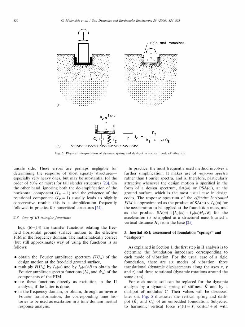
Fig. 5. Physical interpretation of dynamic spring and dashpot in vertical mode of vibration.
G. Mylonakis et al. / Soil Dynamics and Earthquake Engineering 26 (2006) 824–853830
unsafe side. These errors are perhaps negligible fordetermining the response of short squatty structures—especially very heavy ones, but may be substantial (of theorder of 50% or more) for tall slender structures [23]. Onthe other hand, ignoring both the de-amplification of thehorizontal component ðIU ¼ 1Þ and the existence of therotational component ðIF ¼ 1Þ usually leads to slightlyconservative results; this is a simplification frequentlyfollowed in practice for noncritical structures [24].
2.3. Use of KI transfer functions
Eqs. (6)–(14) are transfer functions relating the free-field horizontal ground surface motion to the effectiveFIM in the frequency domain. The mathematically correct(but still approximate) way of using the functions is asfollows:
�
obtain the Fourier amplitude spectrum F(UA) of thedesign motion at the free-field ground surface, � multiply F(UA) by IU(o) and by IF(o)/B to obtain theFourier amplitude spectra functions (UG and FG) of thecomponents of the FIM,
� use these functions directly as excitation in the IIanalysis, if the latter is done,
� in the frequency domain, or obtain, through an inverseFourier transformation, the corresponding time his-tories to be used as excitation in a time domain inertialresponse analysis.
In practice, the most frequently used method involves afurther simplification. It makes use of response spectra
rather than Fourier spectra, and is, therefore, particularlyattractive whenever the design motion is specified in theform of a design spectrum, SA(o) or PSA(o), at theground surface, which is the most usual case in designcodes. The response spectrum of the effective horizontal
FIM is approximated as the product of SAðoÞ � IU ðoÞ forthe acceleration to be applied at the foundation mass, andas the product SAðoÞ � ½IU ðoÞ þ IFðoÞHc=B� for theacceleration to be applied at a structural mass located avertical distance Hc from the base [25].
3. Inertial SSI: assessment of foundation ‘‘springs’’ and
‘‘dashpots’’
As explained in Section 1, the first step in II analysis is todetermine the foundation impedance corresponding toeach mode of vibration. For the usual case of a rigidfoundation, there are six modes of vibration: threetranslational (dynamic displacements along the axes x, y
and z) and three rotational (dynamic rotations around thesame axes).For each mode, soil can be replaced for the dynamic
analysis by a dynamic spring of stiffness K and by adashpot of modulus C. Their values will be discussedlater on. Fig. 5 illustrates the vertical spring and dash-pot (Kz and Cz) of an embedded foundation. Subjectedto harmonic vertical force PzðtÞ ¼ Pz cosðotþ aÞ with
ARTICLE IN PRESSG. Mylonakis et al. / Soil Dynamics and Earthquake Engineering 26 (2006) 824–853 831
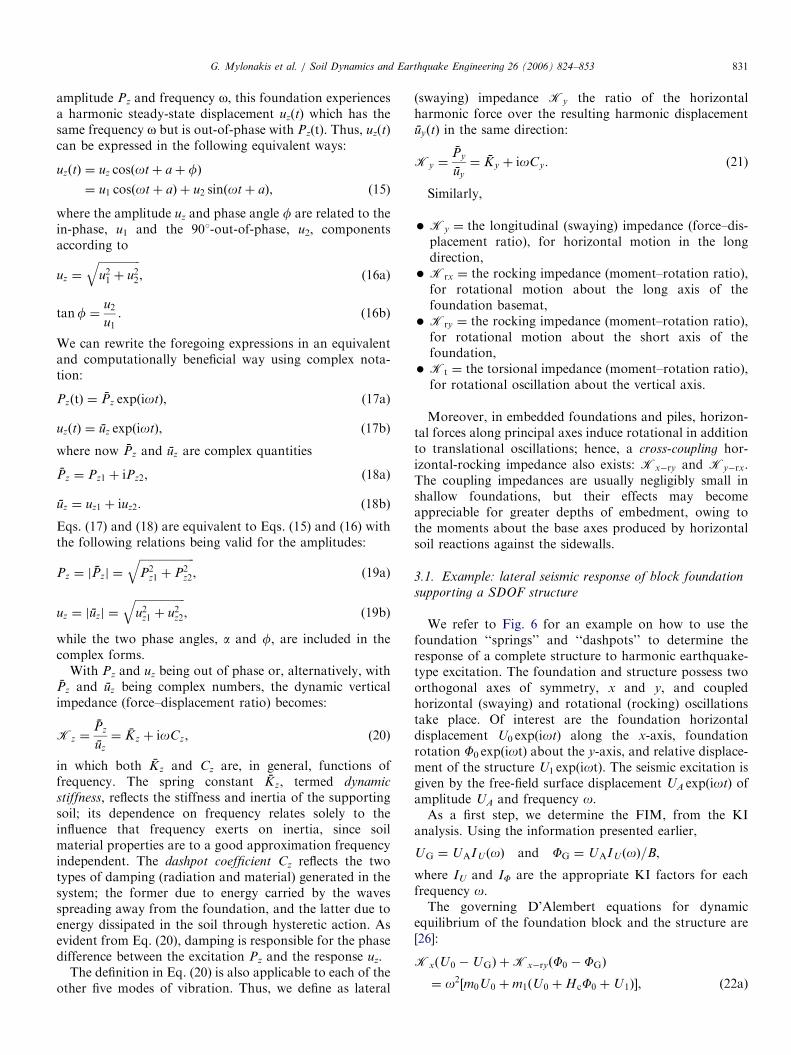
amplitude Pz and frequency o, this foundation experiencesa harmonic steady-state displacement uz(t) which has thesame frequency o but is out-of-phase with Pz(t). Thus, uz(t)can be expressed in the following equivalent ways:
uzðtÞ ¼ uz cosðotþ aþ fÞ
¼ u1 cosðotþ aÞ þ u2 sinðotþ aÞ, ð15Þ
where the amplitude uz and phase angle f are related to thein-phase, u1 and the 901-out-of-phase, u2, componentsaccording to
uz ¼
ffiffiffiffiffiffiffiffiffiffiffiffiffiffiffiu21 þ u2
2
q, (16a)
tanf ¼u2
u1. (16b)
We can rewrite the foregoing expressions in an equivalentand computationally beneficial way using complex nota-tion:
PzðtÞ ¼ Pz expðiotÞ, (17a)
uzðtÞ ¼ uz expðiotÞ, (17b)
where now Pz and uz are complex quantities
Pz ¼ Pz1 þ iPz2, (18a)
uz ¼ uz1 þ iuz2. (18b)
Eqs. (17) and (18) are equivalent to Eqs. (15) and (16) withthe following relations being valid for the amplitudes:
Pz ¼ jPzj ¼
ffiffiffiffiffiffiffiffiffiffiffiffiffiffiffiffiffiffiffiffiP2
z1 þ P2z2
q, (19a)
uz ¼ juzj ¼
ffiffiffiffiffiffiffiffiffiffiffiffiffiffiffiffiffiffiu2
z1 þ u2z2
q, (19b)
while the two phase angles, a and f, are included in thecomplex forms.
With Pz and uz being out of phase or, alternatively, withPz and uz being complex numbers, the dynamic verticalimpedance (force–displacement ratio) becomes:
Kz ¼Pz
uz
¼ Kz þ ioCz, (20)
in which both Kz and Cz are, in general, functions offrequency. The spring constant Kz, termed dynamic
stiffness, reflects the stiffness and inertia of the supportingsoil; its dependence on frequency relates solely to theinfluence that frequency exerts on inertia, since soilmaterial properties are to a good approximation frequencyindependent. The dashpot coefficient Cz reflects the twotypes of damping (radiation and material) generated in thesystem; the former due to energy carried by the wavesspreading away from the foundation, and the latter due toenergy dissipated in the soil through hysteretic action. Asevident from Eq. (20), damping is responsible for the phasedifference between the excitation Pz and the response uz.
The definition in Eq. (20) is also applicable to each of theother five modes of vibration. Thus, we define as lateral
(swaying) impedance Ky the ratio of the horizontalharmonic force over the resulting harmonic displacementuyðtÞ in the same direction:
Ky ¼Py
uy
¼ Ky þ ioCy. (21)
Similarly,
�
Ky ¼ the longitudinal (swaying) impedance (force–dis-placement ratio), for horizontal motion in the longdirection, � Krx ¼ the rocking impedance (moment–rotation ratio),for rotational motion about the long axis of thefoundation basemat,
� Kry ¼ the rocking impedance (moment–rotation ratio),for rotational motion about the short axis of thefoundation,
� Kt ¼ the torsional impedance (moment–rotation ratio),for rotational oscillation about the vertical axis.
Moreover, in embedded foundations and piles, horizon-tal forces along principal axes induce rotational in additionto translational oscillations; hence, a cross-coupling hor-izontal-rocking impedance also exists: Kx�ry and Ky�rx.The coupling impedances are usually negligibly small inshallow foundations, but their effects may becomeappreciable for greater depths of embedment, owing tothe moments about the base axes produced by horizontalsoil reactions against the sidewalls.
3.1. Example: lateral seismic response of block foundation
supporting a SDOF structure
We refer to Fig. 6 for an example on how to use thefoundation ‘‘springs’’ and ‘‘dashpots’’ to determine theresponse of a complete structure to harmonic earthquake-type excitation. The foundation and structure possess twoorthogonal axes of symmetry, x and y, and coupledhorizontal (swaying) and rotational (rocking) oscillationstake place. Of interest are the foundation horizontaldisplacement U0 exp(iot) along the x-axis, foundationrotation F0 exp(iot) about the y-axis, and relative displace-ment of the structure U1 exp(iot). The seismic excitation isgiven by the free-field surface displacement UA exp(iot) ofamplitude UA and frequency o.As a first step, we determine the FIM, from the KI
analysis. Using the information presented earlier,
UG ¼ UAIU ðoÞ and FG ¼ UAIU ðoÞ=B,
where IU and IF are the appropriate KI factors for eachfrequency o.The governing D’Alembert equations for dynamic
equilibrium of the foundation block and the structure are[26]:
KxðU0 �UGÞ þKx�ryðF0 � FGÞ
¼ o2½m0U0 þm1ðU0 þHcF0 þU1Þ�, ð22aÞ

ARTICLE IN PRESS
Fig. 6. Seismic displacements and rotation of a foundation block
supporting a SDOF super-structure. The seismic excitation is described
through the free-field ground-surface displacement UA, assumed to be
produced by a certain type of body or surface waves.
G. Mylonakis et al. / Soil Dynamics and Earthquake Engineering 26 (2006) 824–853832
Kx�ryðU0 �UGÞ þKryðF0 � FGÞ
¼ o2½I0F0 þ I1F0 þm1HcðU0 þHF0 þU1Þ�, ð22bÞ
�m1o2ðU0 þHcF0 þU1Þ þKstrU1 ¼ 0, (22c)
in which m0 and I0 are the mass and mass moment ofinertia of the foundation, m1 and I1 are the mass and massmoment of inertia of the superstructure and Kstr ¼ K str þ
ioCstr the structural impedance (stiffness and damping) ofthe superstructure. Note thatKx�ry is of minor importancein surface foundations, and is usually ommitted.1 Inembedded foundations, however, the term should beincluded, as it may have a profound influence in theresponse [27].
1This holds when the reference system is placed atop the footing ðz ¼ 0Þ,
as is usually the case.
The above equations define a simple algebraic system ofthree equations in three unknowns, despite the fact that thequantities involved are complex numbers. The solution, inmatrix form, for the foundation motion is
U0
F0
( )¼
K
K � o2ðM0 �MbÞ
UG
FG
( ), (23a)
where
K ¼KxKx�ry
Kry�xKry
" #, (23b)
½M0� ¼m0 0
0 I0
" #, (23c)
½Mb� ¼ ½M� þm1
1 Hc
Hc H2c
" #, (23d)
½M� ¼m1 m1Hc
m1Hc m1H2c þ I1
" #(23e)
for the superstructure:
U1 ¼m1o2
K str þ ioCstr �m1o2ðU0 þHcF0Þ. (24)
Eqs. (23) and (24) provide the solution in closed form. Thecomputations, however, may be somewhat tedious ifperformed by hand, since K matrix involves complexnumbers. On the other hand, it is noted that if a real-number notation (with amplitudes and phase angles) hadbeen adopted (as in Eq. (15)), Eqs. (23) would become sixequations with six unknowns—a less desirable procedure.A simple computer code could readily perform theoperations in Eqs. (23) and (24).
3.2. Computing dynamic impedances: tables and charts for
dynamic ‘‘springs’’ and ‘‘dashpots’’
The most important geometric and material factorsaffecting the dynamic impedance of a foundation are:
(1)
the foundation shape (circular, strip, rectangular,arbitrary),(2)
the type of soil profile (deep uniform or multi-layerdeposit, shallow stratum on rock),(3)
the embedment (surface foundation, embedded foun-dation, pile foundation).For a project of critical significance a case-specificanalysis must be performed, using the most suitablenumerical computer program. In most practical cases,however, foundation impedances can be estimated fromapproximate expressions and charts. For the usual case of apractically rigid foundation, a number of analyticalformulae and charts for such stiffnesses have been

ARTICLE IN PRESS
Fig. 7. The four foundation–soil systems whose impedances are given in tabular/graphical form. Numbers I–IV refer to corresponding tables and the
associated graphs.
G. Mylonakis et al. / Soil Dynamics and Earthquake Engineering 26 (2006) 824–853 833
published (e.g., [24,28–35]) and are presented in thissection.
3.3. Surface foundation on homogeneous halfspace
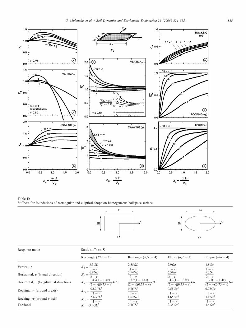
For an arbitrarily-shaped foundation mat, the engineermust first determine an ‘‘equivalent’’ circumscribed rectangle2B by 2L (L4B) using common sense, as sketched in Fig. 7.Then, to compute the impedances in the six modes ofvibration from Table 1a, all that is needed is:
�
Ab, Ibx, Iby, Ib are area, moments of inertia about x, y,and polar moment of inertia about z, of the actual soilfoundation contact surface; if loss of contact under partof the foundation (e.g. along the edges of a rockingfoundation) is likely, engineering judgment may be usedto discount the contribution of this part. � B and L are semi-width and semi length of thecircumscribed rectangle.
� G, n, Vs and VLa, the shear modulus, Poisson’s ratio,shear wave velocity, and ‘‘Lysmer’s analog’’ wavevelocity; the latter is the apparent propagation velocityof compression–extension waves under a foundation
and is related to Vs according to
VLa ¼3:4
pð1� nÞV s. (25)
Additional discussion on the Lysmer analog velocity canbe found in Ref. [33].
� o ¼ cyclic frequency (in rad/s) of interest.This table as well as all other tables in this paper gives:
� the dynamic stiffness (‘‘springs’’), K ¼ KðoÞ as aproduct of the static stiffness, K, times the dynamicstiffness coefficient k ¼ kðoÞ:
KðoÞ ¼ K � kðoÞ, (26)
�
the radiation damping (‘‘dashpot’’) coefficientC ¼ CðoÞ. These coefficients do not include the soilhysteretic damping, b. To incorporate such damping,one should simply add to the foregoing C value thecorresponding material dashpot coefficient 2Kb=o:total C ¼ radiation C þ2Kbo
. (27)
The special cases of footings of rectangular and ellipticshape are addressed in Table 1b.

ARTICLE IN PRESS
Table
1a
Dynamic
stiffnessanddashpotcoefficients
forarbitrary
shaped
foundationsonhomogenoushalfspace
surface
Vibrationmode
Dynamic
stiffnessK¼
KkðoÞ
Radiationdashpotcoefficient
C
Staticstiffness
KDynamic
stiffnesscoefficient
k(G
eneralshapes)
Generalshape
Square
(Generalshape;
0p
a0p2)b
(foundation–soilcontact
surface
area¼
Abwithequivalentrectangle
2L�
2B;
L4
B)a
L¼
B
Vertical,
zK
z¼
2G
L1�nð0:73þ
1:54w0:75Þ
Kz¼
4:54G
B1�n
kz¼
kz
L B;n;a
0
��
Cz¼ðr
VLaA
bÞc
z
withw¼
Ab
4L2
plotted
inGrapha
c z¼
c zL B;a
0
��
plotted
inGraphc
Horizontal,
yK
y¼
2G
L2�nð2þ
2:5w0:85Þ
Ky¼
9G
B2�n
ky¼
ky
L B;a
0
��
Cy¼ðr
VsA
bÞc
y
(lateraldirection)
plotted
inGraphb
c y¼
c yL B;a
0
��
plotted
inGraphd
Horizontal,
xK
x¼
Ky�
0:2
0:75�nG
L1�
B L
��
Kx¼
Ky
kx’
1C
x’
rVsA
b
(longitudinaldirection)
Rocking,rx
(around
xaxis)
Krx¼
G1�n=0:75
bx
L B�� 0:252:4þ0:5
B L
��
Krx¼
0:45G
B3
1�n
krx¼
1�
0:20a0
Crx¼ðr
VLaI
bxÞc
rx
with
I bx¼
areamomentofinertiaoffoundation–soilcontact
surface
around
xaxis
c rx¼
c rx
L B;a
0
��
plotted
inGraphe
Rocking,ry
(around
yaxis)
Kry¼
G1�n=0:75
by
3L B�� 0
:15
hi
Kry¼
Krx
no0:45;
kry’
1�
0:30a0
v’
0:5:
kry’
1�
0:25a0
L B�� 0:30
8 > > > > < > > > > :
Cry¼ðr
VLaI
byÞc
ry
with
I by¼
areamomentofinertiaoffoundation–soilcontact
surface
around
yaxis
c ry¼
c ry
L B;a
0
��
plotted
inGraphf
Torsional
Kt¼
GJ0:75
t4þ
111�
B L
�� 10
hi
Kt¼
8:3
GB3
kt’
1�
0:14a0
Ct¼ðr
VsJ
tÞc t
with
Jt¼
Ib
xþ
Ib
ypolarmomentofinertiaoffoundation–soilcontact
surface
c t¼
c tL B;a
0
��
plotted
inGraphg
aNote
thatas
L=B!1
(strip
footing)thetheoreticalvalues
of
Kzand
Ky!
0;values
computedfrom
thetw
ogiven
form
ulascorrespondto
footingof
L=B�
20.
ba0¼
oB=V
s.
G. Mylonakis et al. / Soil Dynamics and Earthquake Engineering 26 (2006) 824–853834
ARTICLE IN PRESS
Table 1b
Stiffness for foundations of rectangular and elliptical shape on homogeneous halfspace surface
y
x
2L
2B
2a
2bx
y
Response mode Static stiffness K
Rectangle (B=L ¼ 2) Rectangle (B=L ¼ 4) Ellipse (a=b ¼ 2) Ellipse (a=b ¼ 4)
Vertical, z Kz ¼3:3GL
1� n2:55GL
1� n2:9Ga
1� n1:8Ga
1� n
Horizontal, y (lateral direction) Ky ¼6:8GL
2� n5:54GL
2� n6:5Ga
2� n5:3Ga
2� n
Horizontal, x (longitudinal direction) Kx ¼4:9ð1� 1:4nÞð2� nÞð0:75� nÞ
GL3:9ð1� 1:4nÞð2� nÞð0:75� nÞ
GL4:7ð1� 1:37nÞð2� nÞð0:75� nÞ
Ga3:7ð1� 1:4nÞð2� nÞð0:75� nÞ
Ga
Rocking, rx (around x axis) Krx ¼0:82GL3
1� n0:2GL3
1� n0:55Ga3
1� n0:78Ga3
1� n
Rocking, ry (around y axis) Kry ¼2:46GL3
1� n1:62GL3
1� n1:65Ga3
1� n1:1Ga3
1� nTorsional K t ¼ 3:5GL3 2.1GL3 2.35Ga3 1.4Ga3
G. Mylonakis et al. / Soil Dynamics and Earthquake Engineering 26 (2006) 824–853 835

ARTICLE IN PRESSG. Mylonakis et al. / Soil Dynamics and Earthquake Engineering 26 (2006) 824–853836
3.4. Partially and fully embedded foundations
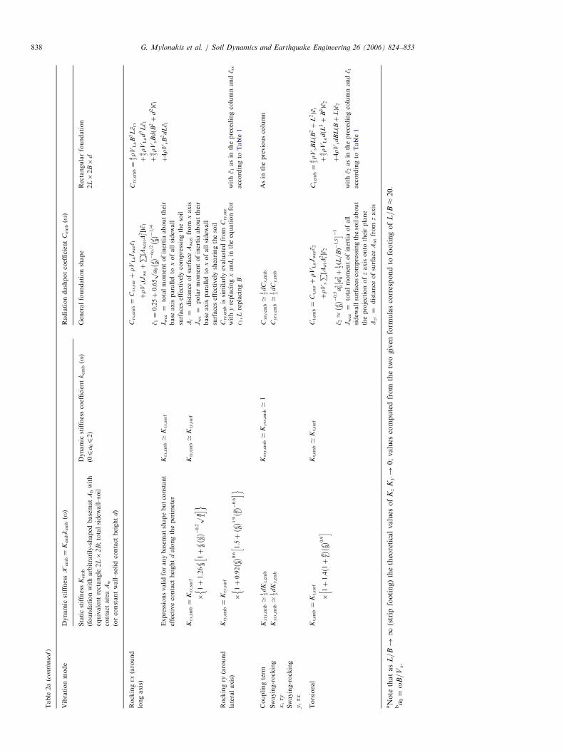
For a foundation embedded in a deep and relativelyhomogeneous soil deposit that can be modeled as ahomogeneous halfspace, springs and dashpots are obtainedfrom the formulae and charts of Table 2a (modified fromGazetas [36]). The foundation basemat can again be ofarbitrary (solid) shape (Fig. 7). The engineer mustdetermine the following additional parameters usingthe table:
�
D is the depth below the ground surface of thefoundation basemat. � Aw or d is the total area of the actual sidewall–soilcontact surface, or the (average) height of the sidewallthat is in good contact with the surrounding soil. Aw
should, in general, be smaller that the nominal area ofcontact to account for such phenomena as slippage andseparation that may occur near the ground surface. Theengineer should refer to published results of large andsmall-scale experiments for a guidance in selecting asuitable value for Aw or d (e.g., [37–40]). Note that Aw ord will not necessarily attain a single value for all modesof vibration.
� Aws and Awce which refer to horizontal oscillations andrepresent the sum of the projections of all the sidewallarea in directions parallel (Aws) and perpendicular (Awce)to loading. Again Aws and Awce should be smaller thanthe nominal areas in shearing and compression, toaccount for slippage and/or separation. h is the distanceof the (effective) sidewall centroid from the groundsurface.
� Note that most of the formulae of Table 2a are valid forsymmetric and nonsymmetric contact along the peri-meter of the vertical sidewalls and the surrounding soil.Note also that Table 2a compares the dynamicstiffnesses and dashpot coefficients of an embeddedfoundation Kemb ¼ Kemb � kemb and Cemb with those ofthe corresponding surface foundation, K sur ¼ K sur �
ksur and Csur.
Approximate solutions for the special cases of footingsof rectangular and elliptic shapes are given in Table 2b.
3.5. Presence of bedrock at shallow depth
Natural soil deposits are frequently underlain by verystiff material or bedrock at a shallow depth, rather thanextending to practically infinite depth as the homogenoushalfspace implies. The proximity of such stiff formation tothe oscillating surface modifies the static stiffness, K, anddashpot coefficients C(o). Specifically, with reference toTable 3 and its charts:
(a) The static stiffnesses in all modes decrease with therelative depth to bedrock H/B. This is evident from allformulae of Table 3, which reduce to the correspondinghalfspace stiffnesses when H/R approaches infinity.
Particularly sensitive to variations in the depth to rockare the vertical stiffnesses—the effect being far morepronounced with strip footings (factor 3.5 versus 1.3).Horizontal stiffnesses are also appreciably affected. On theother hand, for H/R41.5 the response to torsional loads isessentially independent of the layer thickness.As indication of the causes of this different behavior
(between circular and strip footings and, in any footing,between the different types of loading) can be obtained bycomparing the depths of the ‘‘zone of influence’’ in eachcase. Circular and square foundations on a homogeneoushalfspace induce vertical normal stresses sz along thecenterline of the footing that become practically negligibleat depths exceeding 5 footing radii ðzv ¼ 5RÞ; with stripfoundations vertical stresses practically vanish only below15 footing widths ðzv ¼ 15BÞ. The depth of influence, zh, forthe horizontal stresses tzx, due to lateral loading is about2R and 6B for circle and strip, respectively. On the otherhand, for all foundation shapes (strip, rectangle, circle),moment loading is ‘‘felt’’ down to a depth, zr, of about 2B
or 2R. For torsion, finally zt ¼ 0:75R or 0.75B.Apparently when a rigid formation extends into the
‘‘zone of influence’’ of a particular loading mode, iteliminates the corresponding deformations and therebyincreases the stiffness.(b) The variation of the dynamic stiffness coefficients with
frequency reveals an equally strong dependence on the depthto bedrock H/B. On a stratum, k(o) is not a smoothfunction but exhibits undulations (peaks and valleys)associated with the natural frequencies (in shearing andcompression–extension) of the stratum. In other words, theobserved fluctuations are the outcome of resonancephenomena: waves emanating from the oscillating founda-tion reflect at the soil–bedrock interface and return back totheir source at the surface. As a result, the amplitude of thefoundation motion may significantly increase at frequenciesnear the natural frequencies of the deposit. Thus, thedynamic stiffness (being the inverse of displacements)exhibits troughs, which can be very steep when the hystereticdamping of the soil is small (in fact, in certain cases, k(o)would be exactly zero if the soil was ideally elastic).For the ‘‘shearing’’ modes of vibration (swaying and
torsion) the natural fundamental frequency of the stratumwhich controls the behavior of k(o) is
f s ¼V s
4H, (28)
where H denotes the thickness of the layer, while for the‘‘compressing’’ modes (vertical, rocking) the correspondingfrequency is
f c ¼V La
4H¼
3:4
pð1� nÞf s. (29)
(c) The variation of the dashpot coefficient, C, withfrequency reveals a twofold effect on the presence of a rigidbase at relatively shallow depth. First, C(o) also exhibitsundulations (crests and troughs) due to the wave reflections

ARTICLE IN PRESS
Table
2a
Dynamic
stiffnessesanddashpotcoefficients
forarbitrary
shaped
foundationspartiallyorfullyem
bedded
inahomogeneoushalfspace
Vibrationmode
Dynamic
stiffnessK
emb¼
Kem
bkem
b(o
)Radiationdashpotcoefficient
Cemb(o
)
Staticstiffness
Kemb
Dynamic
stiffnesscoefficient
kemb(o
)Generalfoundationshape
Rectangularfoundation
(foundationwitharbitrarily-shaped
basemat
Abwith
equivalentrectangle
2L�
2B;totalsidew
all–soil
contact
area
Aw
ð0p
a0p2Þ
2L�2B�
d
(orconstantwall–solidcontact
height
d)
Vertical
zK
z;em
b¼
Kz;surf
1þ
1 21
D Bð1þ
1:3wÞ
�
np0:4
Cz;em
b¼
Cz;surfþ
rVsA
wC
z;em
b¼
4rV
LaB
Lc z
�1þ
0:2
Aw
Ab� 2=3
��
Fullyem
bedded:
Kz;em
b¼
Kz;surf
1�
0:09
D B�� 3=4
a2 0
hi
Inatrench
Kz;tre¼
Kz;surf
1þ0:09
D B�� 3=4
a2 0
hi
Partiallyem
bedded:
interpolate
betweenthetw
o
8 > > > > > > > > > > < > > > > > > > > > > :
þ4rV
sðBþ
LÞd
Kz,surfobtained
from
Table
1C
z,surf:seeTable
1c z
accordingto
Table
1
Aw¼
actualsidew
all–soildcontact
area;
n¼
0:5
forconstanteffectivecontact
high
dalongthe
perim
eter
Fullyem
bedded;
L=B’
1�
2
Kz;em
b’
1�
0:09
D B�� 3=4
a2 0
Fullyem
bedded;
L=B
43
Kz;em
b’
1�
0:35
D B�� 1=2
a0:35
0
8 > > > > > < > > > > > :A
w¼
d�Perim
eter
w¼
Ab=4
L2
Horizontal
yor
xK
y;emb¼
Ky;surf
1þ
0:15ffiffiffi D Bq
�
Ky;emband
Kx;embcanbeestimatedin
term
of
L/D
,D/B,and
d/B
foreach
a0from
the
grantaccompanyingthistable
Cy;emb¼
Cy;surf
Cy;emb¼
4rV
sB
Lc y
�1þ
0:52
h BAw
L2
� 0:4
��
þrV
sA
wsþrV
LaA
wce
þ4rV
sB
dþ4rV
LsL
d
Ky,surfobtained
from
Table
1A
ws¼P ðA
wisinW iÞ
c yaccordingto
Table
1
Kx;emband
Cx;embare
computedsimilarlyfrom
Kx;surf
and
Cy;surf
¼totaleffectivesidew
allarea
shearingthesoil
Awce¼P ðA
wicosW iÞ
¼totaleffectivesideallarea
compressingthesoil
y¼
inclinationangle
ofsurface
Awifrom
loadingdirection
Cy;surfaccordingto
Table
1
G. Mylonakis et al. / Soil Dynamics and Earthquake Engineering 26 (2006) 824–853 837
ARTICLE IN PRESSTable
2a(c
onti
nued
)
Vibrationmode
Dynamic
stiffnessK
emb¼
Kem
bkem
b(o
)Radiationdashpotcoefficient
Cemb(o
)
Staticstiffness
Kemb
Dynamic
stiffnesscoefficient
kemb(o
)Generalfoundationshape
Rectangularfoundation
(foundationwitharbitrarily-shaped
basemat
Abwith
equivalentrectangle
2L�
2B;totalsidew
all–soil
contact
area
Aw
ð0p
a0p2Þ
2L�2
B�
d
(orconstantwall–solidcontact
height
d)
Rockingrx
(around
longaxis)
Crx;emb¼
Crx;surþ
rVLaIwce
c 1C
rx;emb¼
4 3rV
LaB3L
c rx
þrV
sðJ
wsþP ½A
wceiD
2 i�Þ
c 1þ
4 3rV
Lad3L
c 1
c 1¼
0:25þ
0:65p
a0
d B�� �a0=2
d B�� �1=4
þ4 3rV
sB
dðB
2þ
d2Þc
1
Expressionsvalidforanybasematshapebutconstant
effectivecontact
height
dalongtheperim
eter
Krx;emb’
Krx;surf
I wce¼
totalmomentofinertiaabouttheir
base
axisparallel
toxofallsidew
all
surfaceseffectivelycompressingthesoil
þ4rV
sB2d
Lc 1
Krx;emb¼
Krx;surf
Kry;emb’
Kry;surf
Di¼
distance
ofsurface
Awceifrom
xaxis
�1þ1:26
d B1þ
d Bd D�� �
0:2p
B L
hi
no
Jws¼
polarmomentofinertiaabouttheir
base
axisparallel
toxofallsidew
all
surfaceseffectivelyshearingthesoil
Rockingry
(around
lateralaxis)
Kry;emb¼
Kry;surf
Cry;embissimilarlyevaluatedfrom
Cry;sur
�1þ0:92
d B�� 0:6
1:5þ
d D�� 1:9
B L�� �0:6
hi
no
with
yreplacing
xand,in
theequationfor
c 1;L
replacing
B
with
c 1asin
theprecedingcolumnand
c rx
accordingto
Table
1
Couplingterm
Kxry;emb’
1 3dK
x;emb
Krx
y;emb’
Kyrx;emb’
1C
xry;emb’
1 3dC
x;emb
Asin
thepreviouscolumn
Swaying-rocking
Kyrx;emb’
1 3dK
y;emb
Cyrx;emb’
1 3dC
y;emb
x,ry
Swaying-rocking
y,rx
Torsional
Kt;em
b¼
Kt;surf
Kt;em
b’
Kt;surf
Ct;em
b¼
Ct;surþrV
LaJwce
c 2C
t;em
b¼
4 3rV
sB
LðB
2þ
L2Þc
t
�1þ1:4
1þ
B L
�� d B�� 0
:9h
iþrV
s
P ½AwiD
2 i�c
2þ
4 3rV
LadðL
3þ
B3Þc
2
c 2�
d D�� �0:5
a2 0
a2 0þ
1 2ðL=BÞ�
1:5
� �1
þ4rV
sd
BLðBþ
LÞc
2
Jwce¼
totalmomentofinertiaofall
sidew
allsurfacescompressingthesoilabout
theprojectionof
zaxisonto
theirplane
Dzi¼
distance
ofsurface
Awifrom
zaxis
with
c 2asin
theprecedingcolumnand
c taccordingto
Table
1
aNote
thatas
L=B!1
(strip
footing)thetheoreticalvalues
of
Kz
Ky!
0;values
computedfrom
thetw
ogiven
form
ulascorrespondto
footingof
L=B�
20.
ba0¼
oB=V
s.
G. Mylonakis et al. / Soil Dynamics and Earthquake Engineering 26 (2006) 824–853838

ARTICLE IN PRESSG. Mylonakis et al. / Soil Dynamics and Earthquake Engineering 26 (2006) 824–853 839
at the rigid boundary. These fluctuations are morepronounced with strip than with circular foundations,but are not as significant as for the corresponding stiffnessk(o). Second, and far more important from a practicalviewpoint, is that at low frequencies below the firstresonant (‘‘cutoff’’) frequency of each mode of vibration,radiation damping is zero or negligible for all shapes offootings and all modes of vibration. This is due to thefact that no surface waves can exist in a soil stratumover bedrock at such low frequencies; and, since thebedrock also prevents waves from propagating downward,
the overall radiation of wave energy from the footing isnegligible or nonexistent.Such an elimination of radiation damping may have
severe consequences for heavy foundations oscillatingvertically or horizontally, which would have experiencedsubstantial amounts of damping in a very deep deposit(halfspace)—recall illustrative examples for Tables 1a and2a. On the other hand, since the low-frequency values of C
in rocking and torsion are small even in a halfspace,operating below the cutoff frequencies may not changeappreciably from the presence of bedrock.
ARTICLE IN PRESS
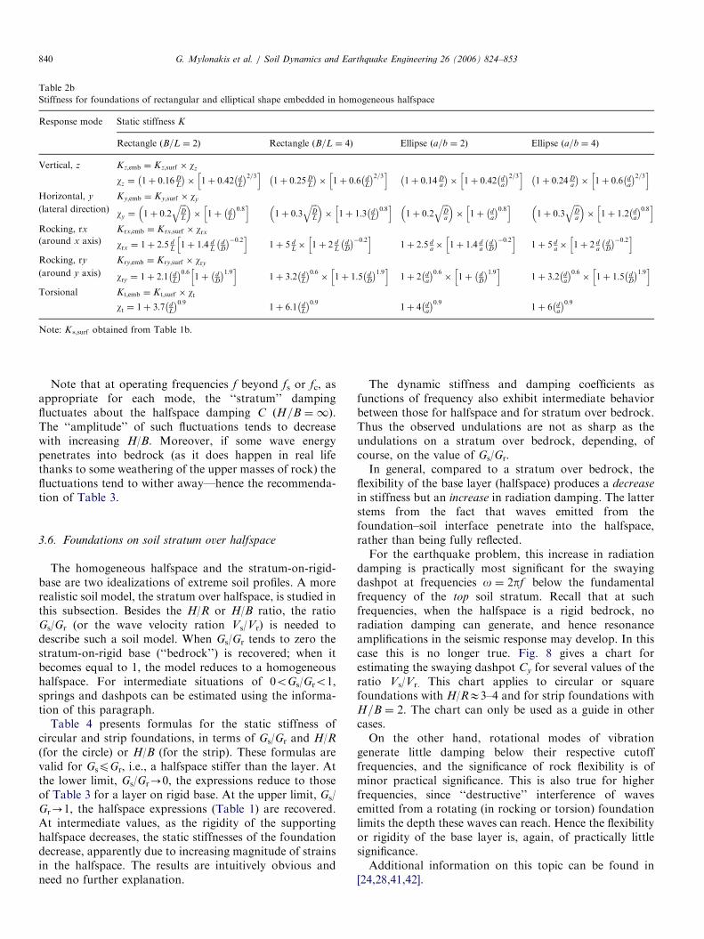
Table 2b
Stiffness for foundations of rectangular and elliptical shape embedded in homogeneous halfspace
Response mode Static stiffness K
Rectangle ðB=L ¼ 2Þ Rectangle ðB=L ¼ 4Þ Ellipse ða=b ¼ 2Þ Ellipse ða=b ¼ 4Þ
Vertical, z Kz;emb ¼ Kz;surf � wz
wz ¼ 1þ 0:16 DL
� �� 1þ 0:42 d
L
� �2=3h i1þ 0:25D
L
� �� 1þ 0:6 d
L
� �2=3h i1þ 0:14 D
a
� �� 1þ 0:42 d
a
� �2=3h i1þ 0:24 D
a
� �� 1þ 0:6 d
a
� �2=3h iHorizontal, y Ky;emb ¼ Ky;surf � wy
(lateral direction) wy ¼ 1þ 0:2ffiffiffiDL
q �� 1þ d
L
� �0:8h i1þ 0:3
ffiffiffiDL
q �� 1þ 1:3 d
L
� �0:8h i1þ 0:2
ffiffiffiDa
q �� 1þ d
a
� �0:8h i1þ 0:3
ffiffiffiDa
q �� 1þ 1:2 d
a
� �0:8h iRocking, rx Krx;emb ¼ Krx;surf � wrx(around x axis) wrx ¼ 1þ 2:5 d
L1þ 1:4 d
LdD
� ��0:2h i1þ 5 d
L� 1þ 2 d
LdD
� ��0:2h i1þ 2:5 d
a� 1þ 1:4 d
adD
� ��0:2h i1þ 5 d
a� 1þ 2 d
adD
� ��0:2h iRocking, ry Kry;emb ¼ Kry;surf � wry(around y axis) wry ¼ 1þ 2:1 d
L
� �0:61þ d
D
� �1:9h i1þ 3:2 d
L
� �0:6� 1þ 1:5 d
D
� �1:9h i1þ 2 d
a
� �0:6� 1þ d
D
� �1:9h i1þ 3:2 d
a
� �0:6� 1þ 1:5 d
D
� �1:9h iTorsional K t;emb ¼ K t;surf � wt
wt ¼ 1þ 3:7 dL
� �0:91þ 6:1 d
L
� �0:91þ 4 d
a
� �0:91þ 6 d
a
� �0:9Note: K�;surf obtained from Table 1b.
G. Mylonakis et al. / Soil Dynamics and Earthquake Engineering 26 (2006) 824–853840
Note that at operating frequencies f beyond fs or fc, asappropriate for each mode, the ‘‘stratum’’ dampingfluctuates about the halfspace damping C ðH=B ¼ 1Þ.The ‘‘amplitude’’ of such fluctuations tends to decreasewith increasing H/B. Moreover, if some wave energypenetrates into bedrock (as it does happen in real lifethanks to some weathering of the upper masses of rock) thefluctuations tend to wither away—hence the recommenda-tion of Table 3.
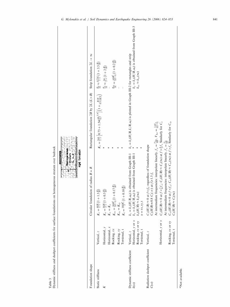
3.6. Foundations on soil stratum over halfspace
The homogeneous halfspace and the stratum-on-rigid-base are two idealizations of extreme soil profiles. A morerealistic soil model, the stratum over halfspace, is studied inthis subsection. Besides the H/R or H/B ratio, the ratioGs/Gr (or the wave velocity ration Vs/Vr) is needed todescribe such a soil model. When Gs/Gr tends to zero thestratum-on-rigid base (‘‘bedrock’’) is recovered; when itbecomes equal to 1, the model reduces to a homogeneoushalfspace. For intermediate situations of 0oGs/Gro1,springs and dashpots can be estimated using the informa-tion of this paragraph.
Table 4 presents formulas for the static stiffness ofcircular and strip foundations, in terms of Gs/Gr and H/R(for the circle) or H/B (for the strip). These formulas arevalid for GspGr, i.e., a halfspace stiffer than the layer. Atthe lower limit, Gs/Gr-0, the expressions reduce to thoseof Table 3 for a layer on rigid base. At the upper limit, Gs/Gr-1, the halfspace expressions (Table 1) are recovered.At intermediate values, as the rigidity of the supportinghalfspace decreases, the static stiffnesses of the foundationdecrease, apparently due to increasing magnitude of strainsin the halfspace. The results are intuitively obvious andneed no further explanation.
The dynamic stiffness and damping coefficients asfunctions of frequency also exhibit intermediate behaviorbetween those for halfspace and for stratum over bedrock.Thus the observed undulations are not as sharp as theundulations on a stratum over bedrock, depending, ofcourse, on the value of Gs/Gr.In general, compared to a stratum over bedrock, the
flexibility of the base layer (halfspace) produces a decrease
in stiffness but an increase in radiation damping. The latterstems from the fact that waves emitted from thefoundation–soil interface penetrate into the halfspace,rather than being fully reflected.For the earthquake problem, this increase in radiation
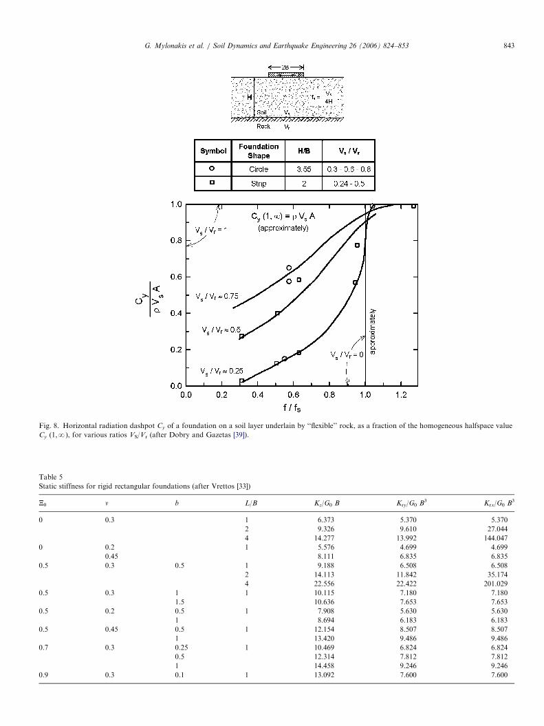
damping is practically most significant for the swayingdashpot at frequencies o ¼ 2pf below the fundamentalfrequency of the top soil stratum. Recall that at suchfrequencies, when the halfspace is a rigid bedrock, noradiation damping can generate, and hence resonanceamplifications in the seismic response may develop. In thiscase this is no longer true. Fig. 8 gives a chart forestimating the swaying dashpot Cy for several values of theratio Vs/Vr. This chart applies to circular or squarefoundations with H/RE3–4 and for strip foundations withH=B ¼ 2. The chart can only be used as a guide in othercases.On the other hand, rotational modes of vibration
generate little damping below their respective cutofffrequencies, and the significance of rock flexibility is ofminor practical significance. This is also true for higherfrequencies, since ‘‘destructive’’ interference of wavesemitted from a rotating (in rocking or torsion) foundationlimits the depth these waves can reach. Hence the flexibilityor rigidity of the base layer is, again, of practically littlesignificance.Additional information on this topic can be found in
[24,28,41,42].
ARTICLE IN PRESS
Table
3
Dynamic
stiffnessanddashpotcoefficients
forsurface
foundationsonhomogeneousstratum
over
bedrock
Foundationshape
Circularfoundationofradius
B¼
RRectangularfoundation2Bby2L(L4
B)
Strip
foundation2L!1
Staticstiffness
Vertical,
zK
z¼
4G
R1�n1þ1:3
R H
��
Kz¼
2G
L1�n
0:73þ
1:54
B L�� 3=4
hi 1þ
B=H
0:5þ
B=L
�
Kz
2L�
0:73
G1�n
1þ3:5
B H
��
KHorizontal,
yK
y¼
8G
R2�n1þ
0:5
R H
��
*K
y
2L�
2G
2�n1þ
2B H
��
Horizontal,
xK
x¼
Ky
*–
Rocking,rx
Krx¼
8G
R3
3ð1�nÞ
1þ0:17
R H
��
*Krx
2L¼
pGB2
2ð1�nÞ
1þ0:2
B H
��
Rocking,ry
Krx¼
Kry
*–
Torsional,t
Kt¼
16G
R3
31þ
0:10
R H
��
*–
Dynamic
stiffnesscoefficient
Vertical,
zk
z¼
kzðH=R;a
0Þisobtained
from
GraphIII-1
kz¼
kzðH=B;L=B;a
0Þisplotted
inGraphIII-2forrectanglesandstrip
k(o
)Horizontal,
yor
xk
y¼
kyðH=R;a
0Þisobtained
from
GraphIII-1
*k
y¼
kyðH=B;a
0Þisobtained
from
GraphIII-3
Rocking,rx
orry
kað
H=R�
kað1Þ
*krx�
krxð1Þ
Torsional,t
a¼
rx;r
y;t
*
Radiationdashpotcoefficient
Vertical,
zC
zðH=BÞ�
0at
fof c;regardless
offoundationshape
C(o
)C
z(H
/B)E
0.8
Cz(N
)at
fX1.5
f c
Atinterm
ediate
frequencies:interpolate
linearly.
fc¼
VLa
4H,
VLa¼
3:4
Vs
pð1�nÞ
Horizontal,
yor
xC
yðH=BÞ�
0at
fo
3 4fs;
CyðH=BÞ�
Cyð1Þat
f4
4 3fsSim
ilarlyfor
Cx
Atinterm
ediate
frequencies:interpolate
linearly.
fs¼
Vs
4H
Rocking,rx
orry
CrxðH=BÞ�
0at
fo
fc;
CrxðH=BÞ�
Crxð1Þat
f4
fcSim
ilarlyfor
Cry
Torsional,t
Ctð
H=B�
Ctð1Þ
*Notavailable.
G. Mylonakis et al. / Soil Dynamics and Earthquake Engineering 26 (2006) 824–853 841

ARTICLE IN PRESS
Table 4
Static stiffness of circular and strip foundations on soil stratum over
halfspace
Vibration mode General expression
K ¼ KðGs=Gr;H=BÞ ¼ Kð1;1Þ � 1þmðB=HÞ1þmðB=HÞðGs=GrÞ
K(1,N) m
Circle Strip
Vertical K 1.3 3.5
Horizontal of homogenous halfspace 0.5 2.0
Torsional 0.17 0.2
G. Mylonakis et al. / Soil Dynamics and Earthquake Engineering 26 (2006) 824–853842
3.7. Effect of soil heterogeneity
The assumption of homogeneous or layered halfspacemay not be realistic in practice, as the soil gets progressivelystiffer with depth, even in uniform deposits. The prime causeis the increase in confining pressure with depth and theassociated increase in low-strain shear modulus. Soilinhomogeneity can be easily treated in dynamic finite-element formulations by dividing the soil into a number ofhomogeneous layers. Yet, such formulations have not beenadequately exploited to study parametrically the dynamicbehavior of foundations [43]. On the other hand, there is aninherent difficulty in applying analytical and semi-analyticalmethods to dynamics of inhomogeneous media, because ofthe difficulties associated with decoupling of the governingequations and solving of the related differential equations
with variable coefficients. As a result, the number ofsolutions available today is limited [32,33,44–47].In this paper information is provided on three specific
cases for which solutions are available:
�
A rectangular footing with side lengths 2L and 2B(L4B) resting on an elastic deposit with shear modulusincreasing with depth as
G ¼ G0 þ ðG1 � G0Þð1� e�bðz=BÞÞ, (30)
where G0 and GN denote the shear moduli at the surfaceand at infinite depth, respectively, and b is a dimension-less inhomogeneity constant. The problem has beenanalysed by Vrettos [33] for the case of vertical androcking oscillations.
� A circular footing of radius R oscillating vertically onelastic soil with shear modulus increasing proportionallyto the square of depth, and Poisson’s ratio n equal to0.25 [32]
G ¼ G0 1þ bz
R
�2. (31)
b is a dimensionless inhomogeneity parameter which canbe determined by fitting pertinent experimental resultsor field data. The corresponding problem of a stripfooting has been solved by Gazetas [46] and is notdiscussed here. This model can simulate deposits with afast increase in elastic modulus. Usually, however, thequadratic G-variation in Eq. (31) is of minor importancefor practical applications.
ARTICLE IN PRESS
Fig. 8. Horizontal radiation dashpot Cy of a foundation on a soil layer underlain by ‘‘flexible’’ rock, as a fraction of the homogeneous halfspace value
Cy (1,N), for various ratios VS/Vr (after Dobry and Gazetas [39]).
Table 5
Static stiffness for rigid rectangular foundations (after Vrettos [33])
X0 n b L/B Kz/G0 B Kry/G0 B3 Krx/G0 B3
0 0.3 1 6.373 5.370 5.370
2 9.326 9.610 27.044
4 14.277 13.992 144.047
0 0.2 1 5.576 4.699 4.699
0.45 8.111 6.835 6.835
0.5 0.3 0.5 1 9.188 6.508 6.508
2 14.113 11.842 35.174
4 22.556 22.422 201.029
0.5 0.3 1 1 10.115 7.180 7.180
1.5 10.636 7.653 7.653
0.5 0.2 0.5 1 7.908 5.630 5.630
1 8.694 6.183 6.183
0.5 0.45 0.5 1 12.154 8.507 8.507
1 13.420 9.486 9.486
0.7 0.3 0.25 1 10.469 6.824 6.824
0.5 12.314 7.812 7.812
1 14.458 9.246 9.246
0.9 0.3 0.1 1 13.092 7.600 7.600
G. Mylonakis et al. / Soil Dynamics and Earthquake Engineering 26 (2006) 824–853 843

ARTICLE IN PRESSG. Mylonakis et al. / Soil Dynamics and Earthquake Engineering 26 (2006) 824–853844
�
Table 6
Values of G/Gmax for soil beneath foundations (from NEHRP-2003 and
EC8)
Spectral response acceleration, SA
p0.10 p0.15 0.20 X0.30
G/Gmax 0.81 0.64 0.49 0.42
The fact that soil stiffness does not appear as variable in this table [e.g., at
least through a soil category] reduces dramatically its usefulness.
A circular footing or radius R oscillating vertically onelastic soil with shear modulus increasing according tothe function [24]
G ¼ G0 1þ bz
R
�n
, (32)
where n and b are dimensionless parameters.
With reference to the profile in Eq. (30), Table 5 presentsresults for static stiffnesses in the vertical and rockingmodes for different values of the soil Poisson’s ratio. In thetable, X0 denotes the dimensionless parameter
X0 ¼ 1�G0
G1, (33)
which is bounded by zero and one. Selected results fordynamic stiffness and dashpots coefficients are presented inFig. 9. The dimensionless frequency factor indicated in thegraph is expressed in terms of the shear wave velocity at thesurface (Vso) (Table 6).
For the footing on the profile described by Eq. (31),dynamic stiffness and dashpot coefficients are depicted inFig. 10. Corresponding static stiffnesses are provided in thepaper by Guzina and Pak [32] and in [48]. It is noted thatmaterial damping in the soil has been ignored in all theabove studies and, thereby, the derived dashpot coefficientspertain only to wave radiation.
The following noteworthy trends can be identified inthese figures:
1. The variation with frequency of dynamic stiffness issmaller in a heterogeneous soil than in a homogeneous soil.
k zz
0.0
0.5
1.0
a0 = ω B / Vso
0.0 0.5 1.0 1.5 2.0
k ry,
krx
0.0
0.5
1.0
Ξo = 0.9, b = 0.1
Ξo = 0.7, b = 0.5
Ξo = 0.7, b = 0.1
Ξo = 0.7, b = 1
Fig. 9. Normalized dynamic stiffness and dashpot coefficients for vertical an
different values of b and X0 (modified from [33]).
In addition, the dynamic stiffness coefficient k generallydecreases with increasing levels of inhomogeneity. Thedifferences, however, are of secondary importance from apractical point of view.2. Radiation damping decreases substantially with
increasing inhomogeneity in the soil. The effect is morepronounced at low frequencies. This decrease is understoodgiven the limited ability of an inhomogeneous medium toradiate waves away from the source [24,45]. At highfrequencies the discrepancies in damping between aninhomogeneous and a homogeneous medium becomesmaller. This can be explained considering that highfrequency (small wavelength) waves emitted from thefoundation ‘‘see’’ the medium as a homogeneous halfspacehaving wave velocity equal to the surface velocity Vso (inshearing) or VLao (in compression–extension). This prop-erty has been utilized in the development of ‘‘cone’’ modelsfor related problems [14,49].
c zz
0.0
0.5
1.0
a0 = ω B / Vso
0.0 0.5 1.0 1.5 2.0
c ry,
crx
0.0
0.5
1.0
d rocking motion of a square foundation on a nonhomogeneous soil for

ARTICLE IN PRESS
Fig. 11. Effect of inhomogeneity on normalized damping for vertical (upper left
vertical motion of circular footing based on Guzina and Pak [32] and Gazeta
Fig. 10. Dynamic spring and dashpot coefficient for a rigid circular
footing on a linear wave-velocity halfspace (modified from [32]).
G. Mylonakis et al. / Soil Dynamics and Earthquake Engineering 26 (2006) 824–853 845
3. A cutoff frequency is apparent in the results for thecircular footing in Fig. 10. As pointed out by Guzina andPak [32], this may not be totally surprising, since the profilecan be regarded as a limiting case of a multi-layeredmedium in which wave reflections can occur at the‘‘interfaces’’ in the vertical direction. An interestingdiscussion on the issue of cutoff frequency is given in [50].To develop further insight on the effect of inhomogene-
ity in radiation damping, Fig. 11 depicts radiation dampingexpressed in terms of the ratio
bijðoÞ ¼oCijðoÞ2K ijðoÞ
. (34)
The above ratio is referred to as ‘‘damping performanceindex’’ and is analogous to the critical damping ratio in thetheory of the single-degree-of-freedom oscillator. In Fig.11, the dramatic decrease in radiation damping resultingfrom soil inhomogeneity becomes clearly evident.
3.8. Effect of soil nonlinearity
In current soil–structure interaction (SSI) practice,nonlinear plastic soil behavior is usually approximatedthrough a series of iterative linear analyses, using soilproperties (moduli and damping ratios) that are consistentwith the level of shearing strains resulting from theprevious analysis [5,52]. These analyses may utilize awealth of available experimental soil data relating thedecrease in (secant) shear modulus and the increase in
) and rocking motion (lower left) of a square footing based on Vrettos [33];
s [51].

ARTICLE IN PRESS
H = 9.5m
H = 30, 83.5m
V = 80, 1 160 m/s60 m/sρβ
ρβ
ρβ
= = 1.8 Mg/m = 10 %
V = 330 m/s = 2.0 Mg/m = 7 %
m = 350 Mg
R
d D
EIc = 3.5 x 10 KN m26
= 5%β
d = 1.3 m
H = 6m
s1
1
1
3
s2
2
2
3
1
2
c
c
elastic rock
V = 1200 m/s = 2.2 Mg/m = 2 %
r
r
r3
Fig. 12. Bridge system studied.
G. Mylonakis et al. / Soil Dynamics and Earthquake Engineering 26 (2006) 824–853846
(effective) damping ratio with increasing amplitude ofshear strain.
Nonlinearities in the free-field soil are treated routinelywith programs such as SHAKE [6,53]. Much less work hasbeen reported on nonlinearities on the dynamic impedancefunctions of footings. In one of the few available studies(e.g., [54–56]), Borja [54] reports that soil nonlinearityresulting from an external harmonic load tends to increasethe foundation motion and generate low-frequency reso-nances even in a homogeneous halfspace. Another inter-esting study has been conducted by Jakub and Roesset [57].In this, the soil is modeled as homogeneous or inhomoge-neous stratum over rigid base with H=B ¼ 1, 2, and 4. ARamber-Osgood model was used to simulate the nonlinearconstitutive relations of soil and iterative linear analyseswere performed. One of the two parameters of the Ramber-Osgood model, r, was kept constant equal to 2, while thesecond one, a, was varied so as to cover a wide range oftypical soil stress–strain relations. In this model, thevariation of secant modulus and effective damping ratiowith stress amplitude is given by
G
G0¼
1
1þ aðt=G0gyÞ, (35a)
b ¼2
3pG
G0
tG0gy
, (35b)
in which G0 is the initial shear modulus for low levels ofstrain; gy a characteristic shear strain, typically rangingfrom 0.0001% to 0.01%; and t the amplitude of theinduced shear stress.
It was concluded that a reasonable approximation to theswaying and rocking impedances of a rigid strip may beobtained from the available linear viscoelastic solutions,provided that the ‘‘effective’’ values of G and b areestimated from Eqs. (35) with
t ¼ tc, (36)
where tc is the statically induced shear stress at a depthequal to 0.50 B, immediately below the foundation edge.Note that the above depth coincides with the depth ofmaximum shear strain under a vertically loaded stripfooting [58].
For design purposes and as a first approximation, wemention here that the average shear modulus for thesoil beneath a footing can be determined accordingthe NEHRP-2003 recommendations, as a function of thedesign seismic coefficient of the structure (Table 4).Alternatively, one may use approximate cone models toderive strain-compatible moduli [14].
4. Parametric study of the seismic response of bridge pier
To answer some of the questions raised earlier, asystematic parametric study was conducted on an idealizedbridge model. One of features of the study relates to theunavoidable soil nonlinearities during strong seismic
excitation. Such nonlinearities are of two types: ‘‘primary’’,arising from the shear-wave induced deformations in thefree-field soil; and ‘‘secondary’’ arising from the stressesinduced by the oscillating foundation. Whereas establishedmethods of analysis are available for handling the formertype of nonlinearities (through equivalent linear or trulynonlinear algorithms), no simple realistic solution is knownfor the latter. The approach described above is adoptedhere and different soil moduli are used for the analysis ofwave-propagation and for the computation of the dynamicstiffnesses, consistent with the overall level of strains atcharacteristic points under the footing. A discussion ofthe aforementioned decoupling of nonlinearity is given inRef. [5].The bridge pier sketched in Fig. 12 is a slightly idealized
version of an actual bridge. It involves a single column bentof height Hc ¼ 6 m and diameter dc ¼ 1:3 m, founded witha 5-m-diameter ðR ¼ 2:5 mÞ footing placed at a depth D ¼
3 m below the ground surface. The axial load carried by thesystem, P ¼ 3500 kN, is typical of a two-lane highwaybridge with a span of about 35m. Considering a shear wave

ARTICLE IN PRESSG. Mylonakis et al. / Soil Dynamics and Earthquake Engineering 26 (2006) 824–853 847
velocity and a mass density for the top layer of 80m/s and2Mg/m3, respectively, and using the approximate relationG/SuE500, the undrained shear strength of the top layer isestimated at about 50 kPa. Accordingly, the static factor ofsafety of the footing is about:
FS �qu
q¼
1:3� 5:14� 50þ 3� 20
3500=ðp� 2:52Þ� 2, (37)
which is a sufficient, although marginal, value for a bridgefooting.
The contact area between sidewalls and surrounding soilwas considered to be either zero (no sidewall–soil contact)or partial sidewall-soil contact over a height d ¼ 0:5D fromthe base.
Results were obtained for excitation by vertical S waves,described through a horizontal ‘‘rock’’outcrop motion.Both harmonic steady-state and time-history analyses wereperformed, in the frequency and time domains, respec-tively. The former were applied to investigate the salientfeatures (SSI period, effective damping) of the dynamicbehavior of the system; the latter were performed to obtain
Fig. 13. Artificial 0.4g motion and corresponding response spectra for 5%
and 10% damping.
predictions of the response to actual motions. In the time-domain analyses, two different excitation time historieswere used, both having a peak horizontal acceleration(PGA) of about 0.40g:
(a)
Fig.
5%
an artificial accelerogram approximately fitted to theNEHRP-94 PGA ¼ 0:4g,
(b)
the Pacoima downstream motion, recorded (on ‘‘softrock’’ outcrop) during the Northridge 1994 earthquake(since the PGA is 0.42g, scaling of this motion was notconsidered necessary).The two motions and their five and ten percent dampedspectra are shown in Figs. 13 and 14. Use of these motions,as ‘‘rock’’ outcrop excitations, is deemed necessary forchecking the limitations (or showing the generality) of ourconclusions. The same set of motions has been used by theauthors in an earlier study of pile-supported bridge piers[27,59].The results presented in this section refer to a bridge with
a top (deck) free to rotate, subjected to the Pacoima 1994
14. Pacoima (1994) motion and corresponding response spectra for
and 10% damping.

ARTICLE IN PRESSG. Mylonakis et al. / Soil Dynamics and Earthquake Engineering 26 (2006) 824–853848
motion, and rigid rock conditions. A second set ofparametric results, which incorporate more general bound-ary conditions, are presented later on.
The harmonic steady state and transient seismic responseof this pier, obtained in a complete analysis, is displayedin Figs. 15 and 16. These results should be comparedwith those in Figs. 17–20, which examine the followingcases:
(a)
no SSI, i.e. the footing is considered as rigidlysupported (Fig. 18)(b)
embedment having partial sidewall contact ðd ¼ 1:5 mÞwith the surrounding soil (Figs. 17 and 19)(c)
no radiation damping, i.e. setting for all modes ofvibration Crad ¼ 0 (Fig. 20)The following conclusions can be drawn:1. Ignoring SSI reduces the fundamental natural period
of the system (from 0.83 to 0.53 s), bringing it closer toresonance with the second-mode natural period of the soildeposit (0.48 s). In addition, the effect of the soil radiationand hysteretic damping on the bridge response disappear.
Fig. 15. Complete solution: harmoni
Naturally, therefore, the resulting no-SSI bridge transferfunctions exhibit a (spurious) sharp and high peak atT ¼ 0:53 s.Moreover, the rock outcrop excitations are richer in the
period region of 0.50 s than of 0.80 s, which accentuates thepeak at T ¼ 0:53 s.As a result, the no-SSI time histories of bridge-deck and
footing accelerations are (Fig. 18), both, nearly two times
larger than those of the complete solution (with SSI).Also of interest is to notice the change in the nature ofthe bridge-deck response time histories: the (largest)peak in the complete solution, at tE4 s, is in unison withthe long-period ground (free field) oscillations occurringafter about 3 s—apparently produced by resonance atthe fundamental period of the soil deposit. The early
part of the free-field ground motion, with much shorterperiods, is a product of ‘‘secondary’’ resonance betweenthe strong short-period early part of the Pacoima–Northridge excitation and the second natural modeof the soil deposit. However, the effect of this part of theground motion on the bridge is obviously completelyinsignificant.
c steady-state transfer functions.
ARTICLE IN PRESS
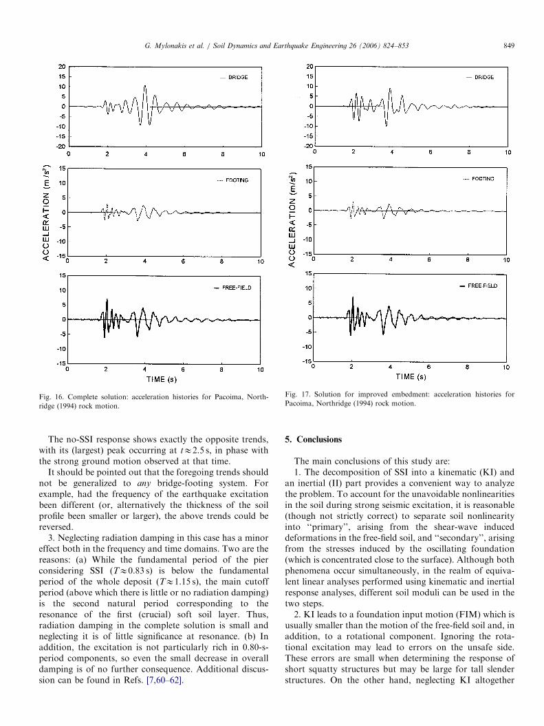
Fig. 16. Complete solution: acceleration histories for Pacoima, North-
ridge (1994) rock motion.
Fig. 17. Solution for improved embedment: acceleration histories for
Pacoima, Northridge (1994) rock motion.
G. Mylonakis et al. / Soil Dynamics and Earthquake Engineering 26 (2006) 824–853 849
The no-SSI response shows exactly the opposite trends,with its (largest) peak occurring at tE2.5 s, in phase withthe strong ground motion observed at that time.
It should be pointed out that the foregoing trends shouldnot be generalized to any bridge-footing system. Forexample, had the frequency of the earthquake excitationbeen different (or, alternatively the thickness of the soilprofile been smaller or larger), the above trends could bereversed.
3. Neglecting radiation damping in this case has a minoreffect both in the frequency and time domains. Two are thereasons: (a) While the fundamental period of the pierconsidering SSI (TE0.83 s) is below the fundamentalperiod of the whole deposit (TE1.15 s), the main cutoffperiod (above which there is little or no radiation damping)is the second natural period corresponding to theresonance of the first (crucial) soft soil layer. Thus,radiation damping in the complete solution is small andneglecting it is of little significance at resonance. (b) Inaddition, the excitation is not particularly rich in 0.80-s-period components, so even the small decrease in overalldamping is of no further consequence. Additional discus-sion can be found in Refs. [7,60–62].
5. Conclusions
The main conclusions of this study are:1. The decomposition of SSI into a kinematic (KI) and
an inertial (II) part provides a convenient way to analyzethe problem. To account for the unavoidable nonlinearitiesin the soil during strong seismic excitation, it is reasonable(though not strictly correct) to separate soil nonlinearityinto ‘‘primary’’, arising from the shear-wave induceddeformations in the free-field soil, and ‘‘secondary’’, arisingfrom the stresses induced by the oscillating foundation(which is concentrated close to the surface). Although bothphenomena occur simultaneously, in the realm of equiva-lent linear analyses performed using kinematic and inertialresponse analyses, different soil moduli can be used in thetwo steps.2. KI leads to a foundation input motion (FIM) which is
usually smaller than the motion of the free-field soil and, inaddition, to a rotational component. Ignoring the rota-tional excitation may lead to errors on the unsafe side.These errors are small when determining the response ofshort squatty structures but may be large for tall slenderstructures. On the other hand, neglecting KI altogether

ARTICLE IN PRESS
Fig. 18. Solution ignoring SSI: acceleration histories for Pacoima,
Northridge (1994) rock motion.
Fig. 19. Solution for improved embedment: harmonic steady-state
transfer function.
G. Mylonakis et al. / Soil Dynamics and Earthquake Engineering 26 (2006) 824–853850
usually leads to slight conservative results. It is thereforerecommended for design of noncritical bridges.
3. In embedded foundations and piles, horizontal forcesinduce rotational, in addition to translational, oscillations,hence a ‘‘cross-coupling’’ horizontal-rocking impedanceexists. Ignoring the coupling stiffness may lead to under-estimation of the fundamental period of a flexibly-supported pier. On the other hand, coupling impedancesare usually small in shallow foundations and can beignored.
4. The contact between the sidewalls of an embeddedfooting and the surrounding soil tends to increase both thestiffness (spring constant) and damping (dashpot constant)of the footing. The actual sidewall area that is in ‘‘good’’contact with the surrounding soil is usually smaller thanthe nominal contact area. The actual contact area does notnecessarily attain a single value for all modes of vibration.
5. If bedrock is present at a shallow depth beneath afooting, the static stiffness in all modes of vibrationincreases. Particularly sensitive to the presence of bedrockis the vertical mode. Horizontal stiffnesses may also beappreciably affected. The torsional and rocking stiffnessesremain essentially unaffected.
6. The variation of dynamic stiffness coefficients is alsosensitive to the presence of bedrock. The amplitude of thefoundation motion may increase significantly at frequen-cies near the natural frequency of the deposit. Radiationdamping is insignificant at frequencies below the ‘‘cutoff’’frequency of the layer. As with their static counterparts,torsional and rocking damping impedances are notparticularly sensitive to the presence of bedrock.7. The dynamic impedances of footings on a soil stratum
overlying a stiffer halfspace exhibit intermediate behaviorbetween those for homogeneous halfspace and for astratum over bedrock. The flexibility of the halfspace leadsto a decrease in stiffness but an increase in radiationdamping. The latter stems from the fact that waves emittedfrom the foundation–soil interface penetrate into thehalfspace rather than being fully reflected. For the earth-quake problem, the increase in radiation damping is mostsignificant in the swaying dashpot, at frequencies below the‘‘cutoff’’ frequency of the stratum.8. It appears difficult to determine a priori whether SSI
will increase or decrease the response of a bridge. In therealm of equivalent linear analyses this seems to becontrolled by the following main parameters: (a) Thesystem damping: if the fundamental period of the flexibly-supported bridge is significantly smaller than the ‘‘cutoff’’frequency of the soil (e.g., a rigid pier on a deep and softdeposit), radiation damping will be significant and theresponse of the system will decrease. In particular, if thecutoff period of the soil is very large (e.g., a thick deposit),

ARTICLE IN PRESS
Fig. 20. Solution neglecting radiation damping: harmonic steady-state transfer functions.
G. Mylonakis et al. / Soil Dynamics and Earthquake Engineering 26 (2006) 824–853 851
radiation damping may be substantial regardless of naturalperiod of the system. This implies that modeling the soil asa halfspace, as done in existing seismic regulations (ATC-3,NEHRP-2003), may lead to unconservative estimates of theresponse. (b) Resonance between structure and soil. If theincrease in fundamental natural period due to SSI bringsthe period of the bridge close to an ‘‘effective’’ naturalperiod (especially the first or second) of the soil, resonancewill develop which will tend to increase the response.However, if the frequency content of the excitation is notrich in that particular period, the increase may beinsignificant. (c) Double resonance. If the fundamentalnatural period of the system coincides with both the naturalperiod of the soil and the predominant period of theearthquake motion (at rock level), double resonance willdevelop (i.e., between structure, soil, and excitation). Inthis case the response may increase dramatically. Whetheror not this will result to damage is related to severaladditional parameters that are not discussed in this study.(d) Nonlinear effects. The development of plastic deforma-tions in the structure and soil, including development ofpore water pressure and uplift, may increase the effectivenatural period of the structure and the soil. This shiftin period may lead to either de-resonance or resonance
(e.g., bringing the structure closer to the predominantperiod of the excitation), which, in turn, may lead to‘‘progressive collapse’’. To date, such strong nonlinearitiesare beyond the state of the art of seismic SSI.The conclusions drawn from the parameter studies
should not be generalized to bridge piers, soil depositsand seismic excitations with characteristics very differentfrom those of the studied cases. However, the observedphenomena and the discussed interplay between variousnatural periods of the system and dominant periods of theground excitation, can be of help in predicting qualitativelythe response in other cases, or in interpreting the results ofnumerical studies.
Acknowledgments
Financial support for this project was provided by theNational Center for Earthquake Engineering Research,FHWA Contract DTFH61-92-C-00112, Task 112-D-3.7.The first author received partial funding from a Car-atheodory grant from University of Patras (D.388). Thanksare also due to Mr. Peter Edinger, Partner, Mueser-Rutledge Consulting Engineers and Professor ChristosVrettos for reviewing the manuscript and offering valuable

ARTICLE IN PRESSG. Mylonakis et al. / Soil Dynamics and Earthquake Engineering 26 (2006) 824–853852
comments, and to the staff of MRCE for preparing someof the drawings. The authors would also like to acknowl-edge the help of Ms. Evangelia Garini in preparing Tables1b and 2b.
References
[1] Kramer S. Geotechnical earthquake engineering. Englewood Cliffs,
NJ: Prentice-Hall; 1996.
[2] Finn WDL. State-of-the-art of geotechnical earthquake engineering
practice. Soil Dyn Earthq Eng 2000;20(1–4):1–15.
[3] Stewart JP, Seed RB, Fenves GL. Seismic soil–structure interaction in
buildings. II: empirical findings. J Geotech Eng ASCE 1999;
125(1):38–48.
[4] Kim S, Stewart JP. Kinematic soil–structure interaction from strong
motion recordings. J Geotech Geoenv Eng ASCE 2003;129(4):
323–35.
[5] Kausel E, Roesset JM, Christian JT. Nonlinear behavior in
soil–structure interaction. J Geotech Eng Div ASCE 1976;102(GT12):
1159–78.
[6] Schnabel PB, Lysmer J, Seed HB. SHAKE: a computer program for
earthquake response analysis of horizontally layered sites. Report
EERC 72-12, University of California, Berkeley, 1972.
[7] Roesset JM. Soil amplification of earthquakes. In: Desai CS,
Christian JT, editors. Numerical methods in geotechnical engineer-
ing. New York: McGraw-Hill; 1977. p. 639–82 [chapter 19].
[8] Elsabee F, Morray JP, Roesset JM. Dynamic behavior of embedded
foundations. Research Report R77-33, MIT, 1977.
[9] Newmark NM, Rosenblueth E. Fundamental of earthquake en-
gineering. Englewood Cliffs, NJ: Prentice-Hall; 640pp.
[10] Luco JE, Westman RA. Dynamic response of circular footings. J Eng
Mech Div ASCE 1971;97(EM5):1381.
[11] Elsabee F, Morray JP, Roesset JM. Dynamic behavior of embedded
foundations. Research Report R77-33, MIT, 1977.
[12] Tassoulas JL. An investigation of the effect of rigid sidewalls on the
response of embedded circular foundations to obliquely-incident SV
and P waves. Dynamic soil–Structure Interaction. Kotterdam: A.A.
Balkemal; 1984. p. 55–63.
[13] Harada T, Kubo K, Katayama T. Dynamic soil–structure interaction
by continuum formulation method. Report No. 190, Institute of
Industrial Science, University of Tokyo, 1981.
[14] Wolf JP. Simple physical models for foundation vibrations. Engle-
wood Cliffs, NJ: Prentice-Hall; 1994.
[15] Gazetas G, Yegian M. Shear and Rayleigh waves in soil dynamics.
ASCE 1979;105(GT12):1455–70.
[16] Gazetas G. Vibrational characteristics of soil depostis with variable
wave velocity. Int J Numer Anal Meth Geomech 1982;6:1–20.
[17] O’Rourke MJ, Bloom M, Dobry R. Apparent propagation velocity
of body waves. Earthq Eng Struct Dyn 1982(10):283–94.
[18] Vrettos C. In-plane vibrations of soil depostis with variable shear
modulus: I. surface waves. Int J Numer Anal Meth Geomech
1990;14:209–22.
[19] Vrettos C. Dispersive SH-surface waves in soil deposits of variable
shear modulus. Soil Dyn Earthq Eng 1990;9:255–64.
[20] Luco JE, Westman RA. Dynamic response of circular footings. J Eng
Mech Div ASCE 1971;97(EM5):1381.
[21] Tassoulas JL. An investigation of the effect of rigid sidewalls on the
response of embedded circular foundations to obliquely-incident SV
and P Waves. Dynamic soil–structure interaction. Rotherdam: A.A.
Balkema; 1984. p. 55–63.
[22] Harada T, Kubo K, Katayama T. Dynamic soil–structure interaction
by continuoum formulation method. Report No 190, Institute of
Industrial Science, University of Tokyo, 1981.
[23] Veletsos AS, Nair VV. Seismic interaction of structures on hysteretic
foundations. J Struct Eng ASCE 1975;101(1):109–29.
[24] Gazetas G. Analysis of machine foundation vibrations: state of the
art. Int J Soil Dyn Earthq Eng 1983;2:2–42.
[25] Gazetas G, Mylonakis G. Seismic soil–structure interaction: new
evidence and emerging issues, emerging issues paper. Geotech Spec
Publ ASCE 1998(75):1119–74.
[26] Richart FE, Hall JR, Woods RD. Vibrations of soils and founda-
tions. Englewood Cliffs, NJ: Prentice-Hall; 1970.
[27] Mylonakis G, Nikolaou A, Gazetas G. Soil–pile–bridge seismic
interaction: kinematic and inertial effects. Part I: soft soil. J Earthq
Eng Struct Dyn 1997;26:337–59.
[28] Luco JE. Impedance functions of a rigid foundation on a layered
medium. Nucl Eng Des 1974;31:204–17.
[29] Kausel E, Roesset JM. Dynamic stiffness of circular foundations.
J Eng Mech Div ASCE 1975;101:771–85.
[30] Wong HL, Luco JE. Tables of impedance functions for square
foundations on layered media. Soil Dyn Earthq Eng 1985;4:64–81.
[31] Dobry R, Gazetas G, Stokoe KH. II Dynamic response of arbitrarily
shaped foundations: experimental verification. J Geotech Eng Div
ASCE 1986;112(2):136–49.
[32] Guzina BB, Pak RYS. Vertical vibration of a circular footing on a
linear-wave-velocity half-space. Geotechnique 1998;48(2):159–68.
[33] Vrettos C. Vertical and rocking impedances for rigid rectangular
foundations on soils with bounded non-homogeneity. Earthq Eng
Struct Dyn 1999;28:1525–40.
[34] Karabalis DL, Beskos DE. Dynamic response of 3-D rigid surface
foundations by time domain boundary element method. Earthq Eng
Struct Dyn 1984;12:73–93.
[35] Qian, Beskos DE. Dynamic interaction between three-dimensional
rigid surface foundations and comparison with the ATC-3 provisions.
Earthq Eng Struct Dyn 1995;24(3):419–37.
[36] Gazetas G. Formulas and charts for impedances of surface and
embedded foundations. J Geotech Eng ASCE 1991;117(9):1363–81.
[37] Stokoe KH, Richart FE. Dynamic response of embedded machine
foundations. J Geotech Eng Div ASCE 1974;100(GT-4):427–47.
[38] Novak M. Experiments with shallow and deep foundations. In:
Gazetas G, Selig ET, editors. Vibration problems in geotechnical
engineering. New York: ASCE; 1985. p. 1–26.
[39] Dobry R, Gazetas G. Dynamic response of arbitrary shaped
foundations. J Geotech Eng Div ASCE 1986;112(2):109–35.
[40] Gazetas G, Stokoe KH. Free vibration of embedded foundations:
theory versus experiment. J Geotech Eng ASCE 1991;117(9):
1382–401.
[41] Hadjian AH, Luco JE. On the importance of layering on impedance
functions. In: Proceedings of the sixth world conference on earth-
quake engineering, New Delhi, 1977.
[42] Gazetas G, Roesset JM. Forced vibrations of strip footing in layered
soils. Method Struct Anal ASCE 1976;1:115–31.
[43] Guzina BB, Pak RYS. Multi-layer representation of continuous
insitu profiles in soil dynamics. Geotechnical special publication, vol.
64. New York: ASCE; 1997. p. 1–10
[44] Awojobi AO. Vertical vibration of a rigid circular foundation on
Gibson soil. Geotechnique 1972;22:333–43.
[45] Awojobi AO. Torsional vibration of a rigid circular body on a non-
homogeneous elastic stratum. Quart J Mech Appl Math 1973;
26:235–47.
[46] Gazetas G. Static and dynamic displacements of foundations on
heterogeneous multilayered soils. Geotechnique 1980;2:159–77.
[47] Muravskii GB. Mechanics of non-homogeneous and anisotropic
foundations. New York: Springer; 2001.
[48] Kassir MK, Chuaprasert MF. A rigid punch in contact with a non-
homogeneous elastic solid. J Appl Mech ASME 1974;41:1019–24.
[49] Meek JW, Veletsos AS. Simple models for foundations in lateral and
rocking motion, Preprints, Fifth world conference on earthquake
engineering. International Association for Earthquake Engineering,
Rome, 1973. 4pp.
[50] Wolf JP. To radiate or not to radiate. Earthq Eng Struct Dyn
1996;25(12):1421–32.
[51] Gazetas G. Foundation vibrations. In: Fang HY, editor. Foundation
engineering handbook. 2nd ed. New York: Van Nostrand Reinholds;
1991. p. 553–93 [chapter 15].

ARTICLE IN PRESSG. Mylonakis et al. / Soil Dynamics and Earthquake Engineering 26 (2006) 824–853 853
[52] Lysmer et al. FLUSH-a computer program of approximate 3-D
analysis of soil–structure interaction problems. Report No. EERC
75-30, University of California, Berkeley; 1975.
[53] Gerolymos N, Gazetas G. Constitutive model for 1–D cyclic soil
behavior applied to seismic analysis of layered deposits. Soils Found
2005;45(3):147–60.
[54] Borja RI, Wu WH. Vibration of foundations on incompressible
soils with no elastic region. J Geotech Eng ASCE 1994;120(9):
1570–92.
[55] Gerolymos N, Escoffier S, Gazetas G, Garnier J. Numerical modeling
of cyclic lateral pile load experiments. J Geotech Geoenv Eng,
submitted for publication.
[56] Gerolymos N, Gazetas G. Phenomenological model applied to
inelastic response of soil–pile interaction systems. Soils Found
2005;45(4):119–32.
[57] Jakub M, Roesset JM. Nonlinear stiffness of foundations. Research
Report R77-35, MIT; 1977.
[58] Tschebotarioff GP. Foundations, retaining and earth structures. 2nd
ed. New York: McGraw-Hill; 1973.
[59] Mylonakis G, Nikolaou A, Gazetas G. Parametric results for seismic
response of pile supported bridge bents. NCEER-95-0021, National
Center for Earthquake Engineering Research, State University of
New York, Buffalo, 1995.
[60] Mylonakis G, Gazetas G. Seismic soil-structure interaction: beneficial
or detrimental? J Earthq Eng 2000;4(3):377–401.
[61] Mylonakis G, Gazetas G, Nikolaou S, Chancey A. Development of
analysis and design procedures for spread footings. Research Report
MCEER-02-0003, Multidisciplinary Center for Earthquake Engineer-
ing Research, State University of New York, Buffalo, 2002. p. 245.
[62] Gerolymos N, Gazetas G, Mylonakis G. Natural period and
damping of bridge-piers on piles. In: Second international conference
in geotechnical earthquake engineering, Lisbon, 1999. p. 299–96.
[63] O’Rourke MJ, Castro G, Hossain I. Horizontal soil strain due to
seismic waves. J Geotech Eng ASCE 1984;110(9):1173–87.