focus of attention and gaze control for robot vision - diva
TRANSCRIPT

Link�oping Studies in Science and Technology. DissertationsNo. 379
Focus of Attention and
Gaze Control for
Robot Vision
Carl-Johan Westelius
Department of Electrical EngineeringLink�oping University, S{581 83 LINK�OPING, Sweden.
Link�oping 1995

ii

Abstract
This thesis deals with focus of attention control in active vision systems.A framework for hierarchical gaze control in a robot vision system is pre-sented, and an implementation for a simulated robot is described. Therobot is equipped with a heterogeneously sampled imaging system, a fovea,resembling the spatially varying resolution of a human retina. The relationbetween foveas and multiresolution image processing as well as implica-tions for image operations are discussed.
A stereo algorithm based on local phase di�erences is presented both asa stand alone algorithm and as a part of a robot vergence control system.The algorithm is fast and can handle large disparities and maintainingsubpixel accuracy. The method produces robust and accurate estimates ofdisplacement on synthetic as well as real life stereo images. Disparity �lterdesign is discussed and a number of �lters are tested, e.g. Gabor �lters andlognorm quadrature �lters. A design method for disparity �lters havingprecisely one phase cycle is also presented.
A theory for sequentially de�ned data modi�ed focus of attention is pre-sented. The theory is applied to a preattentive gaze control system con-sisting of three cooperating control strategies. The �rst is an object �nderthat uses circular symmetries as indications for possible object and directsthe �xation point accordingly. The second is an edge tracker that makesthe �xation point follow structures in the scene. The third is a cameravergence control system which assures that both eyes are �xating on thesame point. The coordination between the strategies is handled usingpotential �elds in the robot parameter space.
Finally, a new focus of attention method for disregarding �lter responsesfrom already modelled structures is presented. The method is based ona �ltering method, normalized convolution, originally developed for �lter-ing incomplete and uncertain data. By setting the certainty of the inputdata to zero in areas of known or predicted signals, a purposive removal ofoperator responses can be obtained. On succeeding levels, image featuresfrom these areas become 'invisible' and consequently do not attract theattention of the system. This technique also allows the system to e�ec-tively explore new events. By cancelling known, or modeled, signals theattention of the system is shifted to new events not yet described.

iv

PREFACE
This thesis is based on the following material:
C-J Westelius, H. Knutsson, and G. H. Granlund. Focus of attentioncontrol. In Proceedings of the 7th Scandinavian Conference on Image
Analysis, pages 667{674, Aalborg, Denmark, August 1991. PatternRecognition Society of Denmark.
C-J Westelius, H. Knutsson, and G. H. Granlund. Preattentive gazecontrol for robot vision. In Proceedings of Third International Con-
ference on Visual Search. Taylor and Francis, 1992.
J. Wiklund, C-J Westelius, and H. Knutsson. Hierarchical phasebased disparity estimation. In Proceedings of 2nd Singapore Inter-
national Conference on Image Processing. IEEE Singapore Section,September 1992.
H. Knutsson, C-F Westin, and C-J Westelius. Filtering of uncer-tain irregularity sampled multidimensional data. In Twenty-seventh
Asilomar Conf. on Signals, Systems & Computers, Paci�c Grove,California, USA, November 1993. IEEE.
G. H. Granlund, H. Knutsson, C-J Westelius, and J Wiklund. Issuesin robot vision. Image and Vision Computing, 12(3):131{148, April1994.
C-J. Westelius and H. Knutsson. Hierarchical disparity estimationusing quadrature �lter phase. International Journal on Computer
Vision, 1995. Special issue on stereo, (submitted).
C-J. Westelius, C-F. Westin, and H. Knutsson. Focus of attentionmechanisms using normalized convolution. IEEE Trans on Robotics
and Automation, 1996. Special section on robot vision. (submitted).
v
vi
Material related to this work but not explicitly reviewed in this
thesis:
C-J Westelius and C-F Westin. Representation of colour in imageprocessing. In Proceedings of the SSAB Conference on Image Anal-
ysis, Gothenburg, Sweden, March 1989. SSAB.
C-J Westelius and C-F Westin. A colour representation for scale-spaces. In The 6th Scandinavian Conference on Image Analysis,pages 890{893, Oulu, Finland, June 1989.
C-J Westelius, G. H. Granlund, and H. Knutsson. Model projec-tion in a feature hierarchy. In Proceedings of the SSAB Sympo-
sium on Image Analysis, pages 244{247, Link�oping, Sweden, March1990. SSAB. Report LiTH{ISY{I{1090, Link�oping University, Swe-den, 1990.
M. G�okstorp and C-J. Westelius. Multiresolution disparity estima-tion. In Proceedings of the 9th Scandinavian conference on Image
Analysis, Uppsala, Sweden, June 1995. SCIA.
J. Karlholm, C-J. Westelius, C-F. Westin, and H. Knutsson. Objecttracking based on the orientation tensor concept. In Proceedings of
the 9th Scandinavian conference on Image Analysis, Uppsala, Swe-den, June 1995. SCIA.
Contributions in books and collections:
C-J Westelius, H. Knutsson J. Wiklund, and C-F Westin. Phase-based disparity estimation. In J.L. Crowley and H. I. Christensen,editors, Vision as Process, pages 179{192, Springer-Verlag, 1994.ISBN 3-540-58143-X.
C-J Westelius, H. Knutsson, and G. Granlund. Low level focus ofattention. In J.L. Crowley and H. I. Christensen, editors, Vision as
Process, pages 157{178, Springer-Verlag, 1994. ISBN 3-540-58143-X.

vii
C-J Westelius, J. Wiklund, and C-F Westin. Prototyping, visual-ization and simulation using the application visualization system.In H. I. Christensen and J.L. Crowley, editors, Experimental En-vironments for Computer Vision and Image Processing, volume 11of Series on Machine Perception and Arti�cial Intelligence, pages33{62. World Scienti�c Publisher, 1994. ISBN 981-02-1510-X.
C-J Westelius. Local Phase Estimation. In G. H. Granlund andH. Knutsson, principal authors, Signal Processing for Computer Vi-sion,pages 259{278. Kluwer Academic Publishers, 1995. ISBN 0-7923-9530-1.

viii

Acknowledgements
Although my name alone is printed on the cover of this thesis, there are anumber of people who, in one way or another, have a part in its realization.
First of all, I would like to thank all the members of the Computer VisionLaboratory for being jolly good fellows. I will miss the weekly chats inthe sauna (and the beer too).
I thank my supervisor, Dr. Hans Knutsson, for his enthusiastic help with-out which this thesis would have been ready much sooner, but with muchpoorer quality. His intuition never cease astonishing me.
I thank Prof. G�osta Granlund for giving me the opportunity to work inhis group and for sharing ideas and visions about vision.
I would like to give Catharina Holmgren a distinguished services medalfor proof-reading this thesis over and over again. It must be extremelyboring to read something you are not interested in and correct the samekind of mistakes all the time.
I thank Dr. Klas Nordberg for taking the time reading and commentingon this thesis. What Catharina did with the language Klas did with thetechnical content.
I would also like to express my gratitude to Dr. Carl-Fredrik Westin, myfriend and colleague, for all his support, both scienti�cally and morally.
My special thanks to everybody in the \Vision as Process" consortium.It has been very stimulating to work with VAP. Many of the activitiesrelated to VAP have made the PhD-studies worthwhile (including theyearly pre-demo-panics).
Finally, there is someone who eventually accepted that \soon" meanssomewhere between now and eternity. Thank you, Brita, for being, forcaring, for loving. I promise: No more PhD-theses for me!

x

Contents
1 INTRODUCTION AND OVERVIEW 1
1.1 Background : : : : : : : : : : : : : : : : : : : : : : : : : : : 1
1.2 Overview : : : : : : : : : : : : : : : : : : : : : : : : : : : : 3
2 LOCAL PHASE ESTIMATION 5
2.1 What is local phase? : : : : : : : : : : : : : : : : : : : : : : 5
2.2 Singular points in phase scale-space : : : : : : : : : : : : : : 11
2.3 Choice of �lters : : : : : : : : : : : : : : : : : : : : : : : : : 13
2.3.1 Creating a phase scale-space : : : : : : : : : : : : : 16
2.3.2 Gabor �lters : : : : : : : : : : : : : : : : : : : : : : 16
2.3.3 Quadrature �lters : : : : : : : : : : : : : : : : : : : 23
2.3.4 Other even-odd pairs : : : : : : : : : : : : : : : : : : 27
2.3.5 Discussion on �lter choice : : : : : : : : : : : : : : : 35
3 PHASE-BASED DISPARITY ESTIMATION 37
3.1 Introduction : : : : : : : : : : : : : : : : : : : : : : : : : : : 37
3.2 Disparity estimation : : : : : : : : : : : : : : : : : : : : : : 38
3.2.1 Computation structure : : : : : : : : : : : : : : : : : 39
3.2.2 Edge extraction : : : : : : : : : : : : : : : : : : : : : 40
3.2.3 Local image shifts : : : : : : : : : : : : : : : : : : : 41
3.2.4 Disparity estimation : : : : : : : : : : : : : : : : : : 41
3.2.5 Edge and grey level image consistency : : : : : : : : 45
3.2.6 Disparity accumulation : : : : : : : : : : : : : : : : 45
3.2.7 Spatial consistency : : : : : : : : : : : : : : : : : : : 46
3.3 Experimental results : : : : : : : : : : : : : : : : : : : : : : 47
3.3.1 Generating stereo image pairs : : : : : : : : : : : : : 48
3.3.2 Statistics : : : : : : : : : : : : : : : : : : : : : : : : 51
3.3.3 Increasing number of resolution levels : : : : : : : : 52
3.3.4 Increasing maximum disparity : : : : : : : : : : : : 58
3.3.5 Combining line and grey level results : : : : : : : : : 63
xi

xii
3.3.6 Results on natural images : : : : : : : : : : : : : : : 753.4 Conclusion : : : : : : : : : : : : : : : : : : : : : : : : : : : 783.5 Further research : : : : : : : : : : : : : : : : : : : : : : : : 79
4 HIERARCHICAL DATA-DRIVEN FOCUS OF ATTEN-
TION 81
4.1 Introduction : : : : : : : : : : : : : : : : : : : : : : : : : : : 814.1.1 Human focus of attention : : : : : : : : : : : : : : : 814.1.2 Machine focus of attention : : : : : : : : : : : : : : 83
4.2 Space-variant sampled image sensors: Foveas : : : : : : : : 844.2.1 What is a fovea? : : : : : : : : : : : : : : : : : : : : 844.2.2 Creating a log-Cartesian fovea : : : : : : : : : : : : 854.2.3 Image operations in a fovea : : : : : : : : : : : : : : 89
4.3 Sequentially de�ned, data modi�ed focus of attention : : : : 894.3.1 Control mechanism components : : : : : : : : : : : : 894.3.2 The concept of nested regions of interest : : : : : : : 91
4.4 Gaze control : : : : : : : : : : : : : : : : : : : : : : : : : : 944.4.1 System description : : : : : : : : : : : : : : : : : : : 944.4.2 Control hierarchy : : : : : : : : : : : : : : : : : : : : 954.4.3 Disparity estimation and camera vergence : : : : : : 964.4.4 The edge tracker : : : : : : : : : : : : : : : : : : : : 974.4.5 The object �nder : : : : : : : : : : : : : : : : : : : : 1054.4.6 Model acquisition and memory : : : : : : : : : : : : 1124.4.7 System states and state transitions : : : : : : : : : : 1134.4.8 Calculating camera orientation parameters : : : : : 119
4.5 Experimental results : : : : : : : : : : : : : : : : : : : : : : 125
5 ATTENTION CONTROL USING NORMALIZED CON-
VOLUTION 129
5.1 Introduction : : : : : : : : : : : : : : : : : : : : : : : : : : : 1295.2 Normalized convolution : : : : : : : : : : : : : : : : : : : : 1305.3 Quadrature �lters for normalized convolution : : : : : : : : 134
5.3.1 Quadrature �lters for NC using real basis functions : 1345.3.2 Quadrature �lters for NC using complex basis func-
tions : : : : : : : : : : : : : : : : : : : : : : : : : : : 1375.3.3 Real or complex basis functions? : : : : : : : : : : : 138
5.4 Model-based habituation/inhibition : : : : : : : : : : : : : : 1455.4.1 Saccade compensation : : : : : : : : : : : : : : : : : 146

xiii
5.4.2 Inhibition of the robot arm in uence on low levelimage processing : : : : : : : : : : : : : : : : : : : : 146
5.4.3 Inhibition of modeled objects : : : : : : : : : : : : : 1495.4.4 Combining certainty masks : : : : : : : : : : : : : : 151
5.5 Discussion : : : : : : : : : : : : : : : : : : : : : : : : : : : : 153
6 ROBOT AND ENVIRONMENT SIMULATOR 155
6.1 General description of the AVS software : : : : : : : : : : : 1556.1.1 Module Libraries : : : : : : : : : : : : : : : : : : : : 158
6.2 Robot vision simulator modules : : : : : : : : : : : : : : : : 1586.3 Example of an experiment : : : : : : : : : : : : : : : : : : : 164
6.3.1 Macro modules : : : : : : : : : : : : : : : : : : : : : 1656.4 Simulation versus reality : : : : : : : : : : : : : : : : : : : : 1696.5 Summary : : : : : : : : : : : : : : : : : : : : : : : : : : : : 170
A AVS PROBLEMS AND PITFALLS 173
A.1 Module scheduling problems : : : : : : : : : : : : : : : : : : 173A.2 Texture mapping problems : : : : : : : : : : : : : : : : : : 175

xiv

1INTRODUCTION AND OVERVIEW
1.1 Background
A traditional view of a computer vision system has been that it is an ana-lyzing system in one end and a responding one in the other as illustrated inFigure 1.1. The analyzing part supplies a model of the three-dimensionalworld derived from two-dimensional images. The world-model is then usedby the responding part for action planning. Vision is considered to be apre-action stage. The vision algorithms have to furnish a world model in�ne detail. Every feature that the action planning system might need hasto be calculated. The close relationship between analysis and response isnot utilized.
Image
Analysis
Response
Generation
Figure 1.1: The classical pipelined structure of a robot vision system.
1
2 INTRODUCTION AND OVERVIEW
As an answer to this, the active vision paradigm has been developed oversome ten years [6, 5, 50, 3, 4]. In short, active vision is based on theability for the perceiving system to purposively change both external andinternal image formation parameters, e.g. �xation point, focal length, etc.Instead of squeezing every bit of information out of every image, the activevision system picks the bits that are easy to estimate in the continuous ow of images. The system adapts its behavior in order to get the bits ofinformation that are important at the moment. This possibility to solveotherwise ill-posed problems, in combination with an appealing similar-ity to biological systems has thrilled the imagination of many researchers(including the author). The problem that arises is how to control the per-ception. How are the purposive actions generated? Clearly, the structurein Figure 1.1 is not appropriate for an active vision system.
The work at the Computer Vision Laboratory at Link�oping University isaimed at an integrated analysis-response system where general responsesare modi�ed by data, and data is actively sought using proper responses[33]. One important property is that su�ciently complex and data-drivenresponses are built up by letting a general response command, invokedfrom higher levels, be modi�ed by processed data entering from lowerlevels, to produce a speci�c command for the speci�c situation in whichthe system currently operates. Action commands also have an impacton input feature extraction and interpretation, e.g. the interpretation ofoptical ow is di�erent when the head is moving from when it is still.
The computing structure can be thought of as a pyramid with sensor in-puts and actuator outputs at the base (Figure 1.2 on the facing page). Theinput information enters the system, and features of increasing abstractionare estimated as the information ows upwards. The particular advantageof this structure is that the output produced from the system leaves thepyramid at the same lowest level as the input enters. This arrangementenables the interaction between input data analysis and output responsesynthesis.
This thesis discusses focus of attention and gaze control for active visionsystems in this context. It should be emphasized that the algorithmsdescribed here are biologically inspired but not an attempt to model bio-logical systems.

1.2 OVERVIEW 3
Levels of informationabstraction
Levels of responsespecification
Sensor inputs Actuator outputs
RealWorld
Figure 1.2: An integrated analysis-response structure. To the left thesignals from the sensor inputs are processed into descriptions of increas-ing abstraction. To the right general response commands are graduallyre�ned into situation speci�c actions.
1.2 Overview
Chapters 2 and 3 deal with estimation of disparity using local phase andare based on [85, 35, 73]. The local phase is explained, its invariancesand equivariances are described, and its behavior in a scale-space is elab-orated on in Section 2.1. A number of di�erent types of phase estimating�lters are described and tested with respect to scale-space behavior in Sec-tion 2.3. In Chapter 3, a hierarchical algorithm for phase-based disparityestimation, that can handle large disparities and still give subpixel accu-racy is described. In Section 3.3, the �lter dependence of the disparityalgorithm behavior is tested and evaluated.
In Chapter 4 a framework for a hierarchical approach to gaze control of arobot vision system is presented, and an implementation on a simulatedrobot is also described. The robot has a three-layer hierarchical gaze con-trol system based on rotation symmetries, linear structures and disparity.It is equipped with heterogeneously sampled imaging systems, foveas, re-sembling the space varying resolution of a human retina. The relation

4 INTRODUCTION AND OVERVIEW
between the fovea and multiresolution image processing is discussed to-gether with implications for image operations. The chapter is based on[75, 76, 35].
Chapter 5 deals with how to implement a habituation function in order toreduce the impact of known or modeled image structures on data drivenfocus of attention. Using a technique termed 'normalized convolution'when extracting the image features allows for marking areas of the inputimage as unimportant. The image features from these areas then become'invisible' and consequently do not attract the attention of the system,which is the desired behavior of a habituation function. Chapter 5 ispublished in [80, 49].
Finally, Chapter 6 describes the robot simulator that is used in the exper-iments throughout this thesis.

2LOCAL PHASE ESTIMATION
2.1 What is local phase?
Most people are familiar with the global Fourier phase. The shift theo-rem, describing how the Fourier phase is a�ected by moving the signal,is common knowledge. But the phase in signal representations based onlocal operations, e.g. lognormal �lters [44], is not so well-known.
The local phase has a number of interesting invariance and equivarianceproperties that makes it an important feature in image processing.
Local phase estimates are invariant to signal energy. The phasevaries in the same manner regardless if there are small or large signalvariations. This feature makes phase estimates suitable for matching,since it reduces the need for camera exposure calibration and illuminationcontrol.
Local phase estimates and spatial position are equivariant. Thelocal phase generally varies smoothly and monotonically with the posi-tion of the signal except for the modulo 2� wrap-around. Section 2.2discusses cases where the local phase behaves di�erently. Furthermore,it is a continuous variable that can measure changes much smaller thanthe spatial quantization, enabling subpixel accuracy without a subpixelrepresentation of image features.
5
6 LOCAL PHASE ESTIMATION
Phase is stable against scaling. It has been shown that phase is stableagainst scaling up to 20 percent [27].
The spatial derivative of local phase estimates is equivariant with
spatial frequency. In high frequency areas the phase changes faster thanin low frequency areas. The slope of the phase curve is therefore steepfor high frequencies. The phase derivative is called local or instantaneousfrequency [10].
There are many ways to approach the concept of local phase. One wayis to start from the analytic function of a signal and design �lters thatlocally estimate the instantaneous phase of the analytical function [10].An alternative approach, used in this chapter, is to relate local phase tothe detection of lines and edges in images. This chapter discusses one-dimensional signals. The extension of the concept of phase into two ormore dimensions is discussed in Section 4.4.
Figure 2.1 on the next page shows the intensity pro�le over a number oflines and edges. The lines and edges are called events in the rest of thischapter. For illustration purposes the ideal step and Dirac functions havebeen blurred more than what corresponds to the normal fuzziness of anaturalistic image. The low pass �lter used is a Gaussian with � = 1:8pixels.
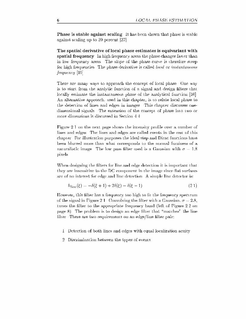
When designing the �lters for line and edge detection it is important thatthey are insensitive to the DC component in the image since at surfacesare of no interest for edge and line detection. A simple line detector is:
hline(�) = ��(� + 1) + 2�(�) � �(� � 1) (2.1)
However, this �lter has a frequency too high to �t the frequency spectrumof the signal in Figure 2.1. Convolving the �lter with a Gaussian, � = 2:8,tunes the �lter to the appropriate frequency band (left of Figure 2.2 onpage 8). The problem is to design an edge �lter that \matches" the line�lter. There are two requirements on an edge/line �lter pair:
1. Detection of both lines and edges with equal localization acuity.
2. Discrimination between the types of events.

2.1 WHAT IS LOCAL PHASE? 7
20 40 60 80 100 120 1400
0.2
0.4
0.6
0.8
1
Inte
nsity
20 40 60 80 100 120 140
Figure 2.1: Intensity pro�les for a bright line on dark background atposition � = 20, an edge from dark to bright at position � = 60, a darkline on bright background at position � = 100, and an edge from bright todark at position � = 140. All lines and edges are ideal functions blurredwith a Gaussian, (� = 1:8).
Is there a formal way to de�ne a line/edge �lter pair such that theserequirements are met?
The answer is yes. In order to see how to generate such a �lter pair,study the properties of lines and edges centered in a window. Setting theorigin to the center of the window reveals that lines are even functions, i.e.f(��) = f(�). Thus, lines have an even real Fourier transform. Edges areodd functions plus a DC term. The DC term can be neglected without lossof generality since neither the line nor the edge �lters should be sensitiveto it. Thus, consider edges simply as odd functions, i.e. f(��) = �f(�),having an odd and imaginary transform.
Now, take a line, fline(�), and an edge, fedge(�), with exactly the samemagnitude function in the Fourier domain,
kFedge(u)k = kFline(u)k: (2.2)
For such signals the line and edge �lter should give identical outputs whenapplied to their respective target events,
Hedge(u)Fedge(u) = Hline(u)Fline(u): (2.3)

8 LOCAL PHASE ESTIMATION
Combining Equations (2.2) and (2.3) gives:
kHedge(u)k = kHline(u)k: (2.4)
Equation (2.4), in combination with the fact that the line �lter is an evenfunction with an even real Fourier transform, while the edge �lter is an oddfunction having an odd and imaginary Fourier transform, shows that anedge �lter can be generated from a line �lter using the Hilbert transformwhich is:
Hedge(u) =
(�iHline(u); if u < 0iHline(u); if u � 0
(2.5)
−10 −5 0 5 10
−0.2
0
0.2
0.4
−10 −5 0 5 10
−0.2
0
0.2
0.4
Figure 2.2: The line detector (left) and its Hilbert transform as edgedetector (right).
The line and edge detectors in Equation (2.5) are both real-valued whichmakes it possible to combine them into a complex �lter with the line �lteras the real part and the edge �lter as the imaginary part:
h(�) = hline(�)� ihedge(�): (2.6)
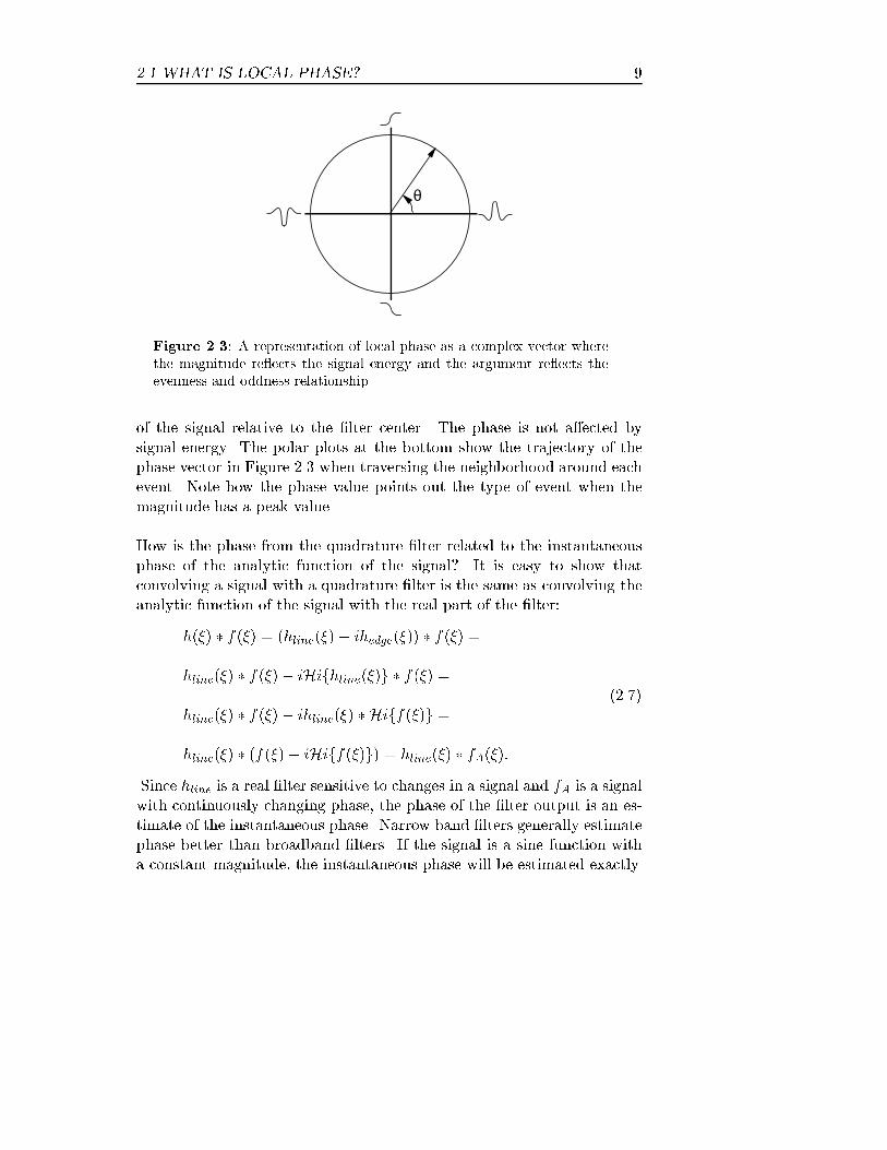
The phase is then represented as a complex value where the magnitude re- ects the signal energy and the argument re ects the relationship betweenthe evenness and oddness of the signal (Figure 2.3).
A �lter ful�lling Equations (2.5) and (2.6) is called a quadrature �lter
and is, in fact, the analytic signal of the line �lter. Figure 2.4 shows thatthe output magnitude from a quadrature �lter depends only on the signalenergy and on how well the signal matches the �lter pass band, and not
on whether the signal is even, odd or a mixture thereof. The �lter phase,on the other hand, depends on the relation between evenness and oddness
2.1 WHAT IS LOCAL PHASE? 9
θ
Figure 2.3: A representation of local phase as a complex vector wherethe magnitude re ects the signal energy and the argument re ects theevenness and oddness relationship.
of the signal relative to the �lter center. The phase is not a�ected bysignal energy. The polar plots at the bottom show the trajectory of thephase vector in Figure 2.3 when traversing the neighborhood around eachevent. Note how the phase value points out the type of event when themagnitude has a peak value.
How is the phase from the quadrature �lter related to the instantaneousphase of the analytic function of the signal? It is easy to show thatconvolving a signal with a quadrature �lter is the same as convolving theanalytic function of the signal with the real part of the �lter:
h(�) � f(�) = (hline(�)� ihedge(�)) � f(�) =
hline(�) � f(�)� iHifhline(�)g � f(�) =
hline(�) � f(�)� ihline(�) � Hiff(�)g =
hline(�) � (f(�)� iHiff(�)g) = hline(�) � fA(�):
(2.7)
Since hline is a real �lter sensitive to changes in a signal and fA is a signalwith continuously changing phase, the phase of the �lter output is an es-timate of the instantaneous phase. Narrow band �lters generally estimatephase better than broadband �lters. If the signal is a sine function witha constant magnitude, the instantaneous phase will be estimated exactly.

10 LOCAL PHASE ESTIMATION
20 40 60 80 100 120 140
20 40 60 80 100 120 1400
0.5
1
20 40 60 80 100 120 140
−3.14
−1.57
0
1.57
3.14
Figure 2.4: Line and edge detection using the quadrature �lter in Fig-ure 2.2 on page 8. Top: The input image. Second: The magnitude of thequadrature �lter output has one peak for each event, and the peak valuedepends only on the signal energy and how well the signal �ts the �lterpass band. Third: The phase of the quadrature �lter output indicatesthe kind of event. Bright lines have � = 0, dark lines have � = �, darkto bright edges have � = �=2, and bright to dark edges have � = ��=2.Bottom: Polar plots showing the phase vector in a neighborhood aroundthe lines and edges.
2.2 SINGULAR POINTS IN PHASE SCALE-SPACE 11
2.2 Singular points in phase scale-space
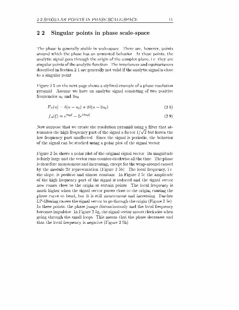
The phase is generally stable in scale-space. There are, however, pointsaround which the phase has an unwanted behavior. At these points, theanalytic signal goes through the origin of the complex plane, i.e. they aresingular points of the analytic function. The invariances and equivariancesdescribed in Section 2.1 are generally not valid if the analytic signal is closeto a singular point.
Figure 2.5 on the next page shows a stylized example of a phase resolutionpyramid. Assume we have an analytic signal consisting of two positivefrequencies u0 and 3u0
FA(u) = �(u � u0) + 2�(u � 3u0) (2.8)
fA(�) = eiu0� + 2ei3u0� (2.9)
Now suppose that we create the resolution pyramid using a �lter that at-tenuates the high frequency part of the signal a factor 1=
p2 but leaves the
low frequency part una�ected. Since the signal is periodic, the behaviorof the signal can be studied using a polar plot of the signal vector.
Figure 2.5a shows a polar plot of the original signal vector. Its magnitudeis fairly large and the vector runs counter-clockwise all the time. The phaseis therefore monotonous and increasing, except for the wrap-around causedby the modulo 2� representation (Figure 2.5b). The local frequency, i.e.the slope, is positive and almost constant. In Figure 2.5c the amplitudeof the high frequency part of the signal is reduced and the signal vectornow comes close to the origin at certain points. The local frequency ismuch higher when the signal vector passes close to the origin, causing thephase curve to bend, but it is still monotonous and increasing. FurtherLP-�ltering causes the signal vector to go through the origin (Figure 2.5e).In these points, the phase jumps discontinuously and the local frequencybecomes impulsive. In Figure 2.5g, the signal vector moves clockwise whengoing through the small loops. This means that the phase decreases andthat the local frequency is negative (Figure 2.5h).

12 LOCAL PHASE ESTIMATION
−2 0 2
−2
0
2
a
0 50 100−3.14
−1.57
0
1.57
3.14 b
−2 0 2
−2
0
2
c
0 50 100−3.14
−1.57
0
1.57
3.14 d
−2 0 2
−2
0
2
e
0 50 100−3.14
−1.57
0
1.57
3.14 f
−2 0 2
−2
0
2
g
0 50 100−3.14
−1.57
0
1.57
3.14 h
Figure 2.5: The periodic signal in Equation (2.9) is LP �ltered in foursteps, attenuating the high frequency part of the signal. The left col-umn shows polar plots of the signal vector and the right column showsthe phase for the same signal. a) The signal vector circles the originat a distance. b) The slope of the phase plot, i.e. the local frequency,is positive and almost constant. c) The signal vector round the originclosely. d) The phase curve bends, which means that the frequency islocally very high. e) The signal vector goes through the origin, i.e. singu-lar points. f) The local frequency is impulsive. g)The the signal vectorgoes trough small loops without rounding the origin. h) The phase curvebends downward which means that the frequency is locally negative.

2.3 CHOICE OF FILTERS 13
This behavior of the phase in scale-space is due to the fact that the high-frequency part of the signal disappears at lower resolution. In Figure 2.5bthe phase has three cycles for each period of the signal since the high-frequency part of the signal dominates. In Figure 2.5h, on the other hand,there is only one phase cycle per signal period since the high-frequencypart is attenuated.
To avoid singular points we can avoid considering points with very lowmagnitude, since the magnitude is zero at the singular points. Unfortu-nately, it is not that simple. The impact of a singular point is spread inscale; negative frequencies on coarser resolution and very high frequencieson �ner resolution. At these points, the magnitude can not be neglectedand a high enough threshold also cuts out many useful phase estimates.Fleet describes how singular points can be detected and how their in uencecan be reduced [26]. A method that uses line images in combination withthe original images to reduce the in uence of singular points is describedin Chapter 3.
2.3 Choice of �lters
When designing �lters to be used as disparity estimators, there are anumber of requirements, some of which are mutually exclusive, to be con-sidered. Di�erent �lter types have di�erent characteristics and which oneto use depends on the application.
There are a number of di�erent �lters that can be used when measuringphase disparities. Gabor �lters are, by far, the most commonly used inphase-based disparity measurement. They have linear phase, i.e. constantlocal frequency, and are therefore intuitively appealing to use. Quadra-ture �lters do not have any negative frequency components nor any DCcomponent. Di�erence of Gaussians approximating the �rst and secondderivative of a Gaussian can also be used to estimate phase.

14 LOCAL PHASE ESTIMATION
0 50 100 150 200 2500
50
100
150
Inte
nsity
Position
Figure 2.6: The signal that is used to test the scale-space behavior ofthe �lters.
Below a number of �lters are evaluated with regard to the following re-quirements:
No DC component. The �lters must not have a DC component. Fig-ure 2.7 on the facing page shows how a DC component makes thesignal vector wag back and forth instead of going round.
No wrap-around. It is desirable, though not necessary, that the phaseof the impulse response runs from �� to � without any wrap around.This maximizes the maximal measurable disparity for a given sizeof the �lter.
Monotonous phase. The phase has to be monotonous, otherwise thephase di�erence between left and right images is not a one-to-onefunction of the disparity. Below, the phase is called monotonouseven though it might wrap around, since the wrap around is causedby the modulo 2� representation.
Only one half-plane of the frequency domain. It is also a requisitethat the �lter only picks up frequencies in one half-plane of the fre-quency domain. This is a quadrature requirement which means thatthe phase must rotate in the same direction for all frequencies. If thisdoes not apply the phase di�erences might change sign dependingon the frequency content of the signal.

2.3 CHOICE OF FILTERS 15
0 50 100 150 200 250
−3
−2
−1
0
1
2
3
U0=0.76 BW=0.5 DC=1.32469e−08
Gab
or fi
lter
phas
e
spatial position
0 50 100 150 200 250
−3
−2
−1
0
1
2
3
U0=0.76 BW=1.2 DC=0.0317708
Gab
or fi
lter
phas
e
spatial position
Figure 2.7: Above, the phase from a Gabor �lter with no DC-component. Below, the phase from a Gabor �lter with broader band-width and thus a DC component on the signal in Figure 2.6. Note thatthe phase is going back and forth instead of wrapping around when thesignal uctuation is small compared the DC level.
In-sensitive to singular points. The area a�ected by the singular pointshas to be as small as possible, both spatially and in scale. As a ruleof thumb the sensitivity to singular points decreases with decreasingbandwidth. This requirement is contradictory to the requirement ofsmall spatial support.
Small spatial support. The computational cost of the convolution isproportional to the spatial support of the �lter function, i.e. the sizeof the �lter, which therefore should be small.

16 LOCAL PHASE ESTIMATION
2.3.1 Creating a phase scale-space
The behavior of the phase in scale-space has been tested using the signalshown in Figure 2.6 on page 14 as input. All �ltering has been done inthe Fourier domain. For each �lter type the DFTs of the �lter with thehighest center frequency have been generated using their de�nitions. Thefrequency function has then been multiplied by a LP Gaussian function:
LP (u) = e� u2
2�2u (2.10)
where �u = �=�2p2�. This emulates the LP-�ltering in a subsampled
resolution pyramid. It can be argued that the LP �ltering should not beused at the highest resolution level, but it can be motivated by taking thesmoothing e�ects of the imaging system into account. The �lter functionfor each level is calculated by scaling the frequency functions appropri-ately:
Fu1(u) = Fu0
�uu0
u1
�(2.11)
Using linear interpolation between nearest neighbors enables non-integerscaling. Again, the method is chosen to resemble a subsampled resolutionpyramid. Generating new �lters for each scale will give better, but larger,�lters, and it will not correspond to a subsampled resolution pyramid.
2.3.2 Gabor �lters
In literature, Gabor �lters are chosen for the minimum space-frequencyuncertainty and for the separability of center frequency and bandwidth.A Gabor �lter tuned to a frequency, u0, is created, spatially, by multiply-ing an envelope function by a complex exponential function with angularfrequency u0 Equation (2.12). Gabor showed that a Gaussian envelopeminimizes the space-frequency uncertainty product [29], a review is foundin [53]. This means that the Gabor �lters are well localized in both do-mains simultaneously.

2.3 CHOICE OF FILTERS 17
−π −3π/4 −π/2 −π/4 0 π/4 π/2 3π/4 π 0
0.2
0.4
0.6
0.8
1
Mag
nitu
de
Frequency
Figure 2.8: The magnitude of three Gabor �lters in the frequency do-main. u0 = f�=8; �=4; �=2g and � = 0:8
When designing a Gabor �lter, the parameters are the standard deviation,�, and the center frequency, u0. These also e�ect the size and the band-width of the �lter. The de�nition of a Gabor �lter in the spatial domainis:
g�u0(�) = ei�u01
�p2�e� �2
2�2 (2.12)
and the de�nition in the frequency domain is:
G�uu0(u) = e� (u�u0)
2
2(�u)2 (2.13)
where �u = 1=�.
The Gabor �lters have linear, and thus monotonous, phase by de�nition.Since the Gaussian has in�nite support in both domains, it is impossibleto keep the �lter in the right half-plane. It is therefore theoretically im-possible to avoid negative frequencies and a DC component. For practicalpurposes the Gaussian can be considered to be zero below some su�cientlylow threshold. The center frequency u0 is connected to the number of pix-els per cycle of the phase and the frequency standard deviation �u isconnected to the spatial and frequency support. By adjusting them, itis possible to get any number of phase cycles over the size of the spatialsupport. But all combinations of u0 and �u do not yield a useful �lter.To see this, suppose that a certain center frequency, u0, is wanted. The
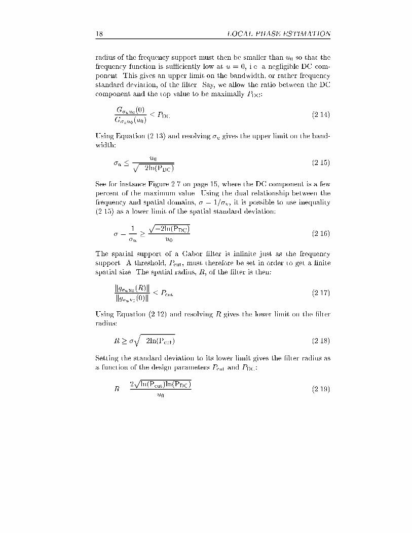
18 LOCAL PHASE ESTIMATION
radius of the frequency support must then be smaller than u0 so that thefrequency function is su�ciently low at u = 0, i.e. a negligible DC com-ponent. This gives an upper limit on the bandwidth, or rather frequencystandard deviation, of the �lter. Say, we allow the ratio between the DCcomponent and the top value to be maximally PDC:
G�uu0(0)
G�uu0(u0)� PDC (2.14)
Using Equation (2.13) and resolving �u gives the upper limit on the band-width:
�u �u0p
�2ln(PDC)(2.15)
See for instance Figure 2.7 on page 15, where the DC component is a fewpercent of the maximum value. Using the dual relationship between thefrequency and spatial domains, � = 1=�u, it is possible to use inequality(2.15) as a lower limit of the spatial standard deviation:
� =1
�u�p�2ln(PDC)
u0(2.16)
The spatial support of a Gabor �lter is in�nite just as the frequencysupport. A threshold, Pcut, must therefore be set in order to get a �nitespatial size. The spatial radius, R, of the �lter is then:
kg�uu0(R)kkg�uu0(0)k
� Pcut (2.17)
Using Equation (2.12) and resolving R gives the lower limit on the �lterradius:
R � �q�2ln(Pcut) (2.18)
Setting the standard deviation to its lower limit gives the �lter radius asa function of the design parameters Pcut and PDC:
R =2pln(Pcut)ln(PDC)
u0(2.19)

2.3 CHOICE OF FILTERS 19
The phase di�erence between the end points of the �lter can now becalculated:
�� = u0R� u0(�R) = 2u0R = 4qln(Pcut)ln(PDC) (2.20)
It should be pointed out that the truncation threshold, Pcut, a�ects the DCcomponent of the �lter. The DC component should therefore be checkedafter truncation of the �lter to see if it is still less than PDC. This was notdone in Table 2.1.
Table 2.1 shows some values on the phase di�erence between the endpoints of the �lter. If the phase di�erence is less than 2� the phase doesnot wrap around.
�� PcutPDC 0.05 0.1 0.2 0.25
0.05 11.982 10.505 8.783 8.151
0.1 10.505 9.210 7.700 7.146
0.2 8.783 7.700 6.437 5.974
0.25 8.151 7.146 5.974 5.545
Table 2.1: Phase di�erence between �lter end points for di�erent valueson the DC component and the truncation threshold. Both PDC and Pcutshould be small. The DC value is not adjusted after truncation of the�lter.
Both PDC and Pcut should be small in order to minimize the DC compo-nent and keep the Gaussian envelope. The conclusion is that having allthe support, or most of it, in the right half-plane of the frequency domain,i.e. a small PDC, requires a center frequency that generates wrap aroundof the phase. Similarly, it can be shown that beginning with a phase thatdoes not wrap around yields a center frequency that is much smaller thanthe frequency support of the �lter. The resulting �lter will then have asubstantial DC component. The upper limit of the relative bandwidth,�, of the Gabor �lters used has heuristically been set to approximately0.8 octaves (Figure 2.8 on page 17). This is also the bandwidth used byFleet et al [27, 39]. Langley suggests that the mean DC level should be

20 LOCAL PHASE ESTIMATION
subtracted from the input images in order to enhance the results [51].The reason is that the DC component of the �lter then is less critical.The best would be to calculate the weighted average in every image pointusing the Gaussian envelope of the Gabor �lter and subtract it from theoriginal image, which is the same as constructing a new �lter without DCcomponent.
The behavior of the Gabor �lters around the singular points has beenthoroughly investigated by Fleet et al [27]. They used a Gabor scale-space function de�ned as
g(�; �) = g�(�)u0(�)(�) (2.21)
where � is the scale parameter. The center frequency decreases when thescale parameter increases, i.e.
u0(�) =2�
�(2.22)
In theory it would be possible to keep the absolute bandwidth constant,i.e. to �xate �u at the standard deviation used at the lowest u0 and thenvary u0. But by doing so, the number of phase cycles over the �lter varieswith the scale. If the relative bandwidth is kept constant, increasing �can be seen as stretching out the same �lter to cover larger areas [32].
Approximating the upper and lower half-height cuto� frequencies as onestandard deviation over and one under the center frequency, i.e.
� = log2u0(�) + �u
u0(�)� �u(2.23)
gives the expression for the spatial standard deviation of the �lter.
�(�) =1
u0(�)
2� + 1
2� � 1
!(2.24)
The isophase curves in Figure 2.9 on page 22 show the phase on a numberof scales. The dark broad lines are due to phase wrap around. A featurethat is stable in scale-space keeps its spatial position in all scales. If the

2.3 CHOICE OF FILTERS 21
phase was completely stable in scale, then the isophase pattern would onlyconsist of vertical lines. The existence of singular points is easily observedin the phase diagram. The positions where the isophase curves convergeare singular points. Just above them, the isophase curves turn downwardsindicating areas with decreasing phase, i.e. negative local frequency, com-pare with Figure 2.5g. The high density of isophase curves just below thesingular points shows that the local frequency is very high (Figure 2.5d).

22 LOCAL PHASE ESTIMATION
50 100 150 200 2500
0.5
1
1.5
2
2.5
3
3.5
4
4.5
Sca
le
Phase of Gabor filter output
50 100 150 200 2500
1
2
3
4
a
Sca
le
Magnitude Gabor filter output
50 100 150 200 2500
1
2
3
4
b
Sca
le
Magnitude less 20% of maximum
50 100 150 200 2500
1
2
3
4
c
Sca
le
Magnitude less 10% of maximum
50 100 150 200 2500
1
2
3
4
d
Sca
le
Magnitude less 5% of maximum
Figure 2.9: Above: Isophase plot of Gabor phase scale-space. Thepositions where the isophase curves converge are singular points. Below:Isomagnitude plot of Gabor phase scale-space. In the dark areas themagnitude is below the threshold. u0 = (�
4)�� and � = 0:8

2.3 CHOICE OF FILTERS 23
2.3.3 Quadrature �lters
Quadrature �lters can be de�ned as having no support in the left half-plane of the frequency domain, and no DC component. This de�nitionmakes them very easy to generate (Equations (2.5) and (2.6)). Thereare number of di�erent types of quadrature �lters of which two will beinvestigated here.
Lognorm �lter
−π −3π/4 −π/2 −π/4 0 π/4 π/2 3π/4 π 0
0.2
0.4
0.6
0.8
1
Mag
nitu
de
Frequency
Figure 2.10: Three lognorm �lters in the frequency domain. u0 =f�=8; �=4; �=2g and � = 0:8
Lognorm �lters are a class of quadrature �lters used for orientation, phaseand frequency estimation [44]. The design parameters are the center fre-quency u0 and the relative bandwidth in octaves, �. The de�nition of thelognorm �lters is in the frequency domain:
F (u) =
(e� 4
log(2)�log2( u
u0)
if u > 00 otherwise
(2.25)
There is, by de�nition, no DC component or any support in the left half-plane of the frequency domain. Although an analytic expression of thespatial de�nition of a lognorm �lter is unavailable, it possible to use someof the results from the Gabor �lter case.
For a certain relative bandwidth the phase goes through a certain numberof cycles independent of the size of the �lter support. Recalling, from the
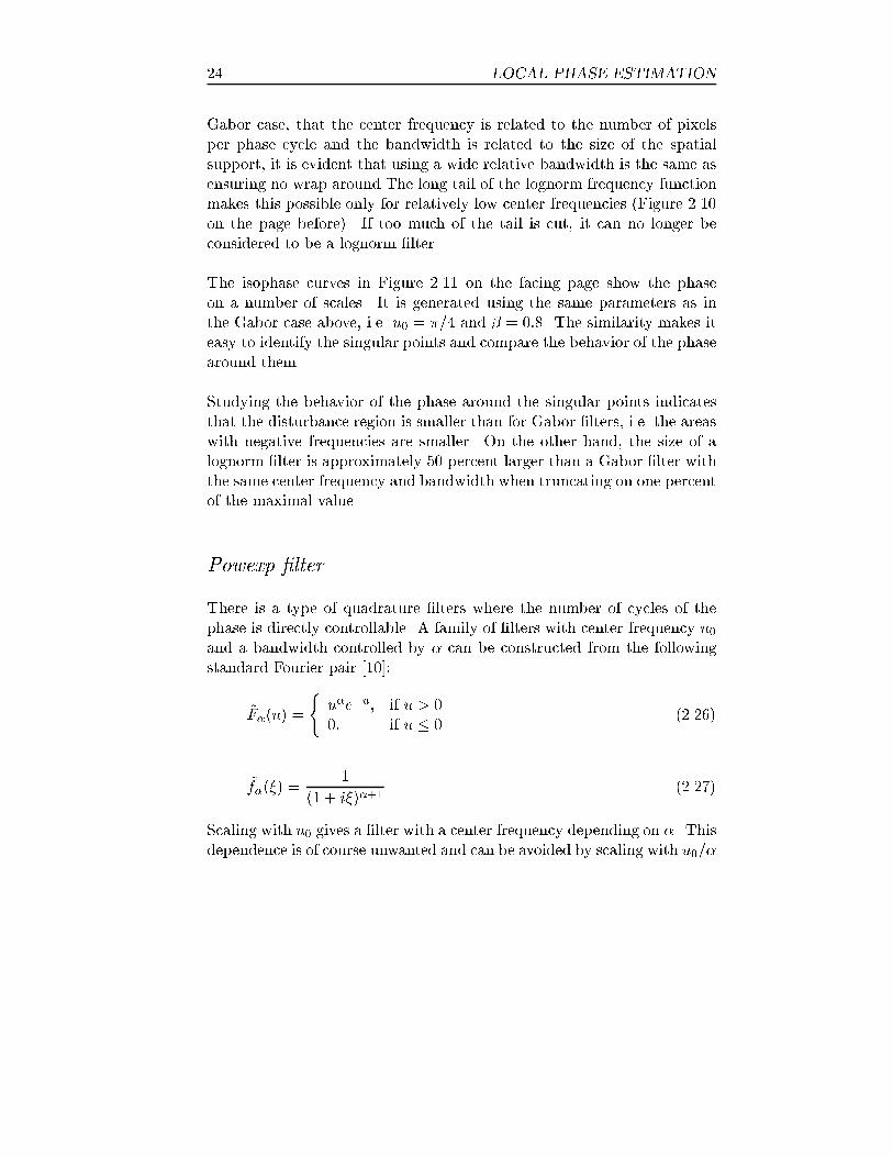
24 LOCAL PHASE ESTIMATION
Gabor case, that the center frequency is related to the number of pixelsper phase cycle and the bandwidth is related to the size of the spatialsupport, it is evident that using a wide relative bandwidth is the same asensuring no wrap around.The long tail of the lognorm frequency functionmakes this possible only for relatively low center frequencies (Figure 2.10on the page before). If too much of the tail is cut, it can no longer beconsidered to be a lognorm �lter.
The isophase curves in Figure 2.11 on the facing page show the phaseon a number of scales. It is generated using the same parameters as inthe Gabor case above, i.e. u0 = �=4 and � = 0:8. The similarity makes iteasy to identify the singular points and compare the behavior of the phasearound them.
Studying the behavior of the phase around the singular points indicatesthat the disturbance region is smaller than for Gabor �lters, i.e. the areaswith negative frequencies are smaller. On the other hand, the size of alognorm �lter is approximately 50 percent larger than a Gabor �lter withthe same center frequency and bandwidth when truncating on one percentof the maximal value.
Powexp �lter
There is a type of quadrature �lters where the number of cycles of thephase is directly controllable. A family of �lters with center frequency u0and a bandwidth controlled by � can be constructed from the followingstandard Fourier pair [10]:
~F�(u) =
(u�e�u; if u > 00; if u � 0
(2.26)
~f�(�) =1
(1 + i�)�+1(2.27)
Scaling with u0 gives a �lter with a center frequency depending on �. Thisdependence is of course unwanted and can be avoided by scaling with u0=�

2.3 CHOICE OF FILTERS 25
50 100 150 200 2500
0.5
1
1.5
2
2.5
3
3.5
4
4.5
Sca
le
Phase of Lognormal filter output
50 100 150 200 2500
1
2
3
4
a
Sca
le
Magnitude of Lognormal filters
50 100 150 200 2500
1
2
3
4
b
Sca
le
Magnitude less 20% of maximum
50 100 150 200 2500
1
2
3
4
c
Sca
le
Magnitude less 10% of maximum
50 100 150 200 2500
1
2
3
4
d
Sca
le
Magnitude less 5% of maximum
Figure 2.11: Above: Isophase plot of Lognorm phase scale-space. Thepositions where the isophase curves converge are singular points. Below:Isomagnitude plot of lognorm phase scale-space. In the dark areas themagnitude is below the threshold. u0 = (�
4)�� and � = 0:8

26 LOCAL PHASE ESTIMATION
instead:
F�u0(u) =
�u0 ��u
u0
��e��uu0 (2.28)
f�u0(�) =1�
1 + iu0��
��+1(2.29)
Finally, normalizing the frequency function gives the wanted Fourier pair:
F�u0(u) =F�u0(u)
F�u0(u0)=
�u
u0
��e��( u
u0�1)
(2.30)
f�u0(�) =1�
1 + iu0��
��+1
1 �u0
��e�� (2.31)
Noting that F�u0(u) = (F1u0(u))�, it is easy to see that the center fre-
quency of the �lter is independent of � and that the bandwidth will de-crease with increasing �. It is equally easy to see that the number of phasecycles of these �lters is a function of �.
For � = 1, the relative bandwidth is approximately two octaves and thephase cycles once. However, both the frequency and spatial support ofthe �lter are very large, which reduces the usefulness of the �lter type. Asan example the spatial support is approximately 60 percent larger thana lognorm �lter with the same center frequency and bandwidth whentruncating at one percent of the maximum value.
2.3 CHOICE OF FILTERS 27
2.3.4 Other even-odd pairs
The �lters described above all consist of an even real part and an oddimaginary part and the phase is calculated from the ratio between theseparts. There are a few other types of �lters that are neither Gabor norquadrature �lters, but which can be interpreted as odd-even pairs.
Non-ringing �lters
−π −3π/4 −π/2 −π/4 0 π/4 π/2 3π/4 π 0
0.2
0.4
0.6
0.8
1
Mag
nitu
de
Frequency
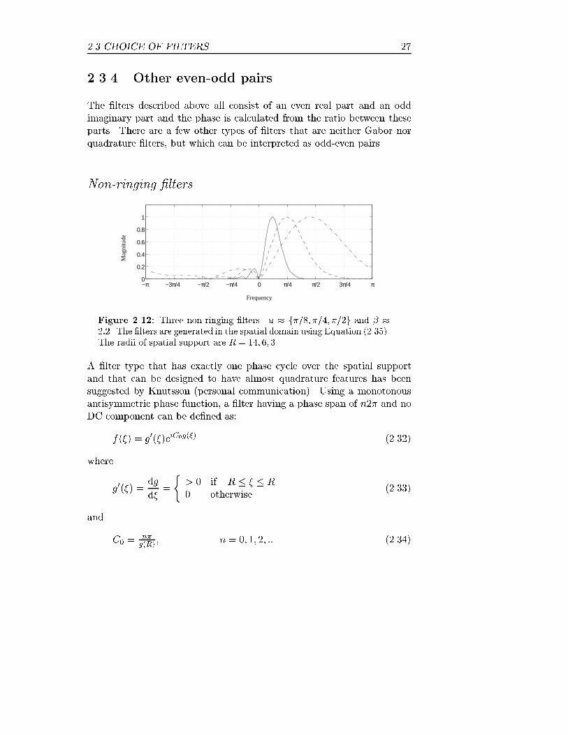
Figure 2.12: Three non-ringing �lters. u � f�=8; �=4; �=2g and � �2:2. The �lters are generated in the spatial domain using Equation (2.35).The radii of spatial support are R = 14; 6; 3.
A �lter type that has exactly one phase cycle over the spatial supportand that can be designed to have almost quadrature features has beensuggested by Knutsson (personal communication). Using a monotonousantisymmetric phase function, a �lter having a phase span of n2� and noDC component can be de�ned as:
f(�) = g0(�)eiC0g(�) (2.32)
where
g0(�) =dg
d�=
(> 0 if �R � � � R
0 otherwise(2.33)
and
C0 =n�g(R)
, n = 0; 1; 2; :: (2.34)
28 LOCAL PHASE ESTIMATION
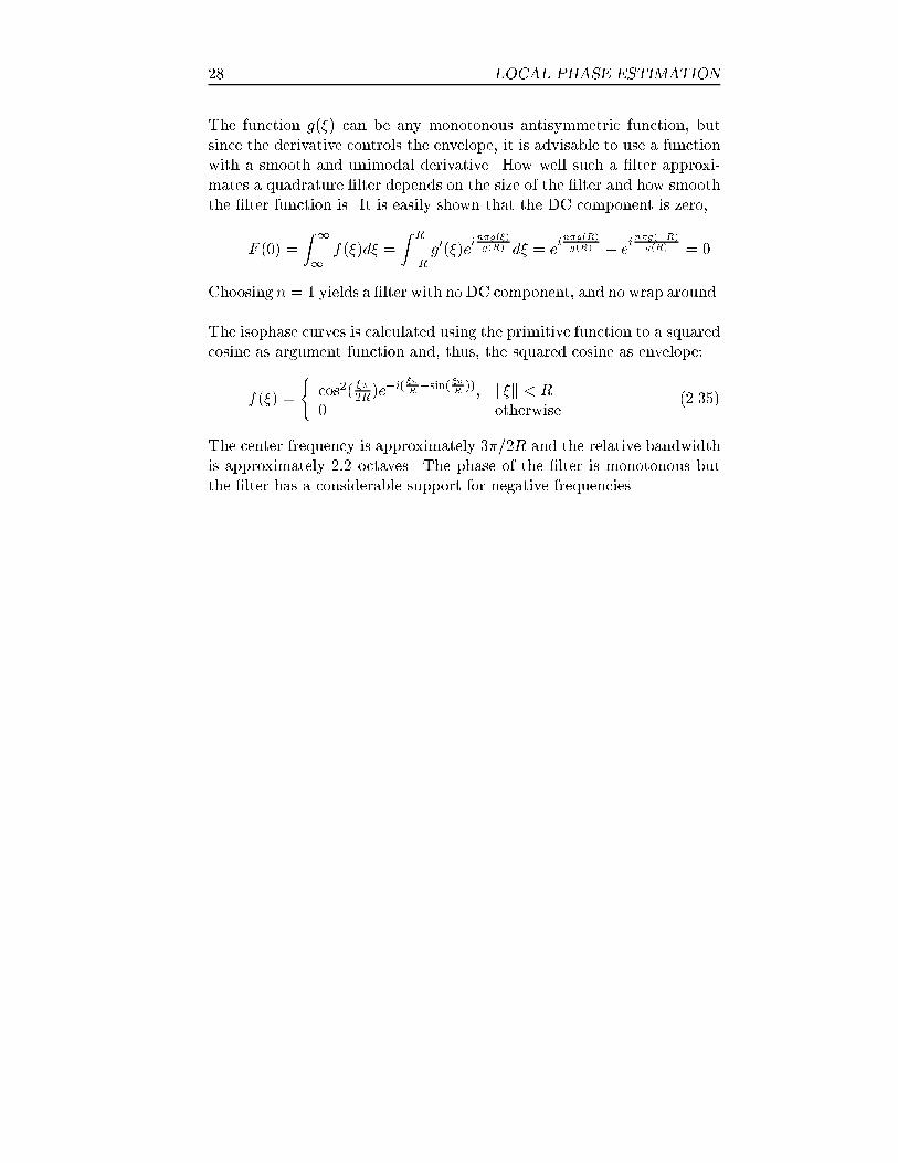
The function g(�) can be any monotonous antisymmetric function, butsince the derivative controls the envelope, it is advisable to use a functionwith a smooth and unimodal derivative. How well such a �lter approxi-mates a quadrature �lter depends on the size of the �lter and how smooththe �lter function is. It is easily shown that the DC component is zero,
F (0) =
Z 1
1f(�)d� =
Z R
�Rg0(�)ei
n�g(�)
g(R) d� = ein�g(R)
g(R) � ein�g(�R)
g(R) = 0
Choosing n = 1 yields a �lter with no DC component, and no wrap around.
The isophase curves is calculated using the primitive function to a squaredcosine as argument function and, thus, the squared cosine as envelope:
f(�) =
(cos2( ��
2R )e�i( ��
R+sin(
��
R)); k�k < R
0 otherwise(2.35)
The center frequency is approximately 3�=2R and the relative bandwidthis approximately 2:2 octaves. The phase of the �lter is monotonous butthe �lter has a considerable support for negative frequencies.

2.3 CHOICE OF FILTERS 29
50 100 150 200 2500
0.5
1
1.5
2
2.5
3
3.5
4
4.5
Sca
le
Phase of Non-ringing filter output
50 100 150 200 2500
1
2
3
4
a
Sca
le
Magnitude of Non-ringing filters
50 100 150 200 2500
1
2
3
4
b
Sca
le
Magnitude less 20% of maximum
50 100 150 200 2500
1
2
3
4
c
Sca
le
Magnitude less 10% of maximum
50 100 150 200 2500
1
2
3
4
d
Sca
le
Magnitude less 5% of maximum
Figure 2.13: Above: Isophaseplot of non-ringing phase scale-space. Thepositions where the isophase curves converge are singular points. Below:Isomagnitude plot of non-ringing phase scale-space. In the dark areasthe magnitude is below the threshold. u0 = (�
4)��

30 LOCAL PHASE ESTIMATION
Windowed Fourier Transform
−π −3π/4 −π/2 −π/4 0 π/4 π/2 3π/4 π 0
0.2
0.4
0.6
0.8
1
Mag
nitu
de
Frequency
Figure 2.14: Three windowed Fourier transform �lters. u =f2�=15; 2�=7; 2�=4g and � = 2:0. The �lters where generated in thespatial domain using Equation (2.36). The radii of spatial support whereR = 7; 3; 2.
The windowed Fourier transform can used for estimating local phase. Thewindow can be chosen arbitrarily, e.g. a rectangular function. Weng ad-vocates the rectangular window [71], which is actually a special case ofthe non-ringing �lters. The spatial magnitude function is a rectangularfunction and the argument is a ramp:
f(�) =
(e�i�
�
R ; k�k < R
0 otherwise(2.36)
Although the term windowed Fourier transform is not tied to any par-ticular window function, �lters de�ned according to Equation (2.36) arecalled WFT �lters in this thesis. Figure 2.14 shows three WFT �lters inthe Fourier domain. The long tails of ripples make the �lter sensitive tohigh-frequency noise. Weng suggests a pre�ltering of the signal with aGaussian, which is the same as a smoothing of the �lter. The resulting�lter is then very similar to the non-ringing �lter above.
The signal is pre�ltered with a smoothing function as described in Sub-section 2.3.1. Any further smoothing is therefore not necessary in thistest.

2.3 CHOICE OF FILTERS 31
50 100 150 200 2500
0.5
1
1.5
2
2.5
3
3.5
4
4.5
Sca
le
Phase of WFT filter output
50 100 150 200 2500
1
2
3
4
a
Sca
le
Magnitude of WFT filters
50 100 150 200 2500
1
2
3
4
b
Sca
le
Magnitude less 20% of maximum
50 100 150 200 2500
1
2
3
4
c
Sca
le
Magnitude less 10% of maximum
50 100 150 200 2500
1
2
3
4
d
Sca
le
Magnitude less 5% of maximum
Figure 2.15: Above: Isophaseplot of WFT phase scale-space. Thepositions where the isophase curves converge are singular points. Below:Isomagnitude plot of WFT phase scale-space. In the dark areas themagnitude is below the threshold. u0 = (�
4)��

32 LOCAL PHASE ESTIMATION
Gaussian di�erences
Gaussian �lters and their derivatives, or rather di�erences, can be e�-ciently implemented using binomial �lter kernels [18]. The basic kernelsare a LP kernel and a di�erence kernel (Figure 2.16). These can be im-plemented using shifts and summations. The �rst and second di�erenceof the binomial Gaussians can be used as a phase estimator (Figure 2.16).The spatial support is only 5 pixels.
Figure 2.16: Left, the LP kernel. Middle, the �rst di�erence kernel, f�.Right, the second di�erence kernel, f��.
−π −3π/4 −π/2 −π/4 0 π/4 π/2 3π/4 π 0
0.2
0.4
0.6
0.8
1
Mag
nitu
de
Frequency
Figure 2.17: The DFT magnitude of the binomial phase �lter for � =0:5 (dot-dashed), � = 0:3333 (dashed) and � = 0:3660 (solid).
From the design, it is evident that there is no DC component and thatthe phase does not wrap around. The �rst di�erence �lter, f�, is the oddkernel, and changing sign on the second di�erence, f��, gives the evenkernel. Instead of just using the kernels as they are, it is possible give

2.3 CHOICE OF FILTERS 33
them di�erent relative weights, producing a range of �lters:
f(�) = ��f�� + i(1� �)f�; where 0 � � � 1 (2.37)
The energy in the left half-plane of the frequency domain is minimizedby setting � = 0:3660 (Figure 2.17 on the preceding page). This designmethod is a special case of a method for producing quadrature �lters calledprolate spheroidals. In the general case, there are an arbitrary number ofbasis �lters that are weighted together, using a multi-variable optimizingtechnique. The method produces the best possible quadrature �lter of agiven size in the sense that it has minimum energy in the left half plane.
If it is essential to the implementation to use only summations and shifts,the weights can be chosen to 1 for f�� and 2 for f�, corresponding to� = 0:3333. The relative bandwidth is approximately two octaves andonly slightly dependent on �.

34 LOCAL PHASE ESTIMATION
50 100 150 200 2500
0.5
1
1.5
2
2.5
3
3.5
4
4.5
Sca
le
Phase of Gaussian differences filter output
50 100 150 200 2500
1
2
3
4
a
Sca
le
Magnitude of Gaussian differences
50 100 150 200 2500
1
2
3
4
b
Sca
le
Magnitude less 20% of maximum
50 100 150 200 2500
1
2
3
4
c
Sca
le
Magnitude less 10% of maximum
50 100 150 200 2500
1
2
3
4
d
Sca
le
Magnitude less 5% of maximum
Figure 2.18: Above: Isophase plot of Gaussian di�erences phase scale-space. The positions where the isophase curves converge are singularpoints. Below: Isomagnitude plot of Gaussian derivatives phase scale-space. In the dark areas the magnitude is below the threshold. u0 =(�2)��
2.3 CHOICE OF FILTERS 35
2.3.5 Discussion on �lter choice
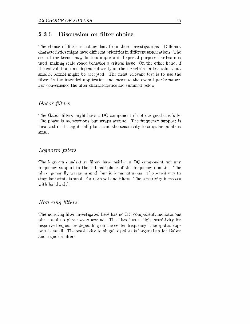
The choice of �lter is not evident from these investigations. Di�erentcharacteristics might have di�erent priorities in di�erent applications. Thesize of the kernel may be less important if special purpose hardware isused, making scale space behavior a critical issue. On the other hand, ifthe convolution time depends directly on the kernel size, a less robust butsmaller kernel might be accepted. The most relevant test is to use the�lters in the intended application and measure the overall performance.For convenience the �lter characteristics are summed below.
Gabor �lters
The Gabor �lters might have a DC component if not designed carefully.The phase is monotonous but wraps around. The frequency support islocalized in the right half-plane, and the sensitivity to singular points issmall.
Lognorm �lters
The lognorm quadrature �lters have neither a DC component nor anyfrequency support in the left half-plane of the frequency domain. Thephase generally wraps around, but it is monotonous. The sensitivity tosingular points is small, for narrow band �lters. The sensitivity increaseswith bandwidth.
Non-ring �lters
The non-ring �lter investigated here has no DC component, monotonousphase and no phase wrap around. The �lter has a slight sensitivity fornegative frequencies depending on the center frequency. The spatial sup-port is small. The sensitivity to singular points is larger than for Gaborand lognorm �lters.

36 LOCAL PHASE ESTIMATION
(Rectangular) Window Fourier Transform
Being a special case of the non-ring �lters, the WFT �lters share theproperties described above. The sensitivity to singular points is the largestof the tested �lters. The smoothing of the �lter that is necessary to reducethe noise in uence makes the �lter very similar to the non-ring �lter basedon the squared cosine magnitude.
Di�erence of Gaussians
Gaussian derivatives �lters implemented with binomial coe�cients do nothave any DC component. The phase is monotonous and there is no phasewrap around. The sensitivity for negative frequencies can be adjusted byweighing the even and odd kernels appropriately. It can, however, not bereduced to zero. The sensitivity to singular points is slightly larger thanfor non-ring �lters. The spatial support is small.

3PHASE-BASED DISPARITY
ESTIMATION
3.1 Introduction
The problem of estimating depth information from two or more images ofa scene is one which has received considerable attention over the years anda wide variety of methods have been proposed to solve it [8, 24]. Methodsbased on correlation and methods using some form of feature matchingbetween the images have found most widespread use. Of these, the latterhave attracted increasing attention since the work of Marr [54], in whichthe features are zero-crossings on varying scales. These methods share anunderlying basis of spatial domain operations.
In recent years, however, increasing interest has been shown in computa-tional models of vision based primarily on a localized frequency domainrepresentation - the Gabor representation [29, 2], �rst suggested in thecontext of computer vision by Granlund [32].
In [63, 87, 40, 27, 51] it is shown that such a representation also can beadapted to the solution of the stereopsis problem. The basis for the successof these methods is the robustness of the local Gabor-phase di�erences.The algorithm presented here is an extension of the work presented in [87].
37

38 PHASE-BASED DISPARITY ESTIMATION
Position1ξ
2
Intensity
ξ
0
π
π/2
−π
−π/2
Phase
Positionξ1
ξ2
∆θ
∆ξ
Figure 3.1: Left: A superimposed stereo image pair of a line. In the leftimage the line is located at �1 (solid) and in the right image it is locatedat �2. Right: The phase curves corresponding to the line in the twoimages. The displacement �� can be estimated by calculating the phasedi�erence, ��, and the slope of the phase curve, i.e. the local frequencyd�=d�.
3.2 Disparity estimation
The fact that phase is locally equivariant with position can be used toestimate local displacement between two images [63, 87, 25, 72]. In astereo image pair the local displacement is a measure of depth and in animage sequence the local displacement is an estimate of velocity.
One of the advantages of using phase for displacement estimation is thatsubpixel accuracy can be obtained without having to change the samplingdensity. Figure 3.1 shows an example where the displacement of a line ina stereo image pair is estimated using phase di�erences. Traditional dis-placement estimation would calculate the position of a signi�cant feature,e.g. the local maximum of the intensity, and then calculate the di�er-ence. If subpixel accuracy is needed the feature locations would have tobe stored using some sort of subpixel representation.
The local phase, on the other hand, is a continuous variable sensitive tochanges much smaller than the spatial quantization. Sampling the phasefunction with a certain density does not restrict the phase di�erences

3.2 DISPARITY ESTIMATION 39
SpatialCons.
ShiftDisparity
esti
mation
Shift
Shift
Shift
Accu-mulator
SpatialCons.
Edgedetect.
Leftimage
Rightimage
Edgedetect.
Figure 3.2: Computation structure for the hierarchical stereo algorithm.
to the same accuracy. Thus, a subpixel displacement generates a phaseshift giving phase di�erences with subpixel accuracy without a subpixelrepresentation of image features. In Figure 3.1 the displacement estimateis:
�� =��
�0(3.1)
3.2.1 Computation structure
A hierarchical stereo algorithm that uses a phase based disparity estimatorhas been developed [84]. To optimize the computational performance, amultiresolution representation of the left and right image is used. An edgedetector, tuned to vertical structures, is used to produce a pair of imagescontaining edge information. The edge images reduces the in uence ofsingular points since the singular points in the original images and theedge images generally do not coincide. The impact of a DC componentin the disparity �lter is also reduced be means of the edge images. The

40 PHASE-BASED DISPARITY ESTIMATION
edge images together with the corresponding original image pair are usedto build the resolution pyramids. It is one octave between the levels. Thenumber of levels needed depends on the maximum disparity in the stereoimage pair.
The algorithm starts at the coarsest resolution. The disparity accumu-lator holds and updates disparity estimates and con�dence measures foreach pixel. The four input images are shifted locally according to thecurrent disparity estimates. After the shift, a new disparity estimate iscalculated using the phase di�erences, the local frequency and their con-�dence values. The disparity estimate from the edge image pair has highcon�dence close to edges, while the con�dence is low in between them.The estimates from the original image pair resolve possible problems ofmatching incompatible edges, that is, only edges with the same sign of thegradient should be matched. Both these disparity estimates are weightedtogether by a consistency function to form the disparity measure betweenthe shifted images. The new disparity measure updates the current esti-mate in the disparity accumulator. For each resolution level a re�nementof the disparity estimate can be done by iterating these steps. It shouldget closer and closer to zero during the iterations.
Between each level the disparity image is resampled to the new resolution,and a local spatial consistency check is performed. The steps above arerepeated until the �nest resolution is reached. The accumulator imagethen contains the �nal disparity estimates and certainties.
3.2.2 Edge extraction
Creating edge images can be done using any edge extraction algorithm.Here the edge extraction is performed using the same �lter as for thedisparity estimation. The magnitude of the �lter response is stored inthe edge image, creating a sort of line drawing. The disparity �lters aresensitive only to more or less vertically oriented structures, but this is nolimitation since horizontal lines does not contain any disparity informa-tion. The produced edge image is used as input to create a resolutionpyramid in the same way as described above. There are a total of fourpyramids that are generated before starting the disparity estimation.

3.2 DISPARITY ESTIMATION 41
3.2.3 Local image shifts
The images from the current level in the resolution pyramid are shiftedaccording to the disparity accumulator, which is initialized to zero. Theleft and right images are shifted half the distance each. The shift proceduredecreases the disparity since the left and right images are shifted towardseach other. It reduces di�erences due to foreshortening as well [61]. Thismeans that if a disparity is estimated fairly well at a coarse resolution,the reduction of the disparity will enable the next level to further re�nethe result.
The shift is implemented as a \picking at a distance" procedure:
xsL(�1; �2) = xL(�1 + 0:5��; �2) (3.2)
xsR(�1; �2) = xR(�1 � 0:5��; �2) (3.3)
which means that a value is picked from a the old image to the new imageat a distance determined by the disparity, ��. This ensures that there willbe no points without a value. Linear interpolation between neighboringpixels allow non-integer shifts.
3.2.4 Disparity estimation
The disparity is measured on both the grey level images and the edgeimages. The phase can be estimated using any of the �lters described inSection 2.3. The result will of course vary with the the �lter character-istics, but a number of consistency checks reduces the variation between�lter types.
The disparity is estimated in the grey level images and the edge imagesseparately and the results are weighted together. The �lter responses in apoint can be represented by a complex number. The real and imaginaryparts of the complex number represents the even and odd �lter responsesrespectively. The magnitude is a measure of how strong the signal is andhow well it �ts the �lter. The magnitude will therefore be used as acon�dence measure of the �lter response. The argument of the complexnumber is the phase in the signal.

42 PHASE-BASED DISPARITY ESTIMATION
Let the responses from the phase estimating �lter be represented with thecomplex numbers zL and zR for the left and right image respectively. The�lters are normalized so that 0 � kzL;Rk � 1. Calculating
d = zLzR�; (3.4)
where � denotes the complex conjugate, yields a phase di�erence measureand a con�dence value,
kdk = kzLkkzRk; 0 � kdk � 1 (3.5)
arg(d) = arg(zL)� arg(zR); �� � arg(d) � � (3.6)
The magnitude, kdk, is large only if both �lter magnitudes are large.It consequently indicates how reliable the phase di�erence is. If a �ltersees a completely homogeneous neighborhood, its magnitude is zero andits argument is unde�ned. Calculating the phase di�erence without anycon�dence values then produces an arbitrary result.
If the images are captured under similar conditions and they are coveringapproximately the same area, it is reasonable that the magnitudes of the�lter responses are approximately the same for both images. This canbe used to check the validity of the disparity estimate. A substantialdi�erence in magnitude can be due to noise or too large disparity, i.e. theimage neighborhoods do not depict the same part of reality. It can also bedue to a singular point in one of the signals, since the magnitude is reducedconsiderably in such neighborhoods. In any of these cases the con�dencevalue of the estimate should be reduced, so the consistency checks lateron can weigh the estimate accordingly. Sanger used the ratio between thesmaller and the larger of the magnitudes as a con�dence value [63]. Sucha con�dence value does not di�erentiate between strong and weak signals.The con�dence function below depends both on the relation between the�lter magnitudes and the absolute value. The con�dence value thereforere ects both the similarity and the signal strength:
C1 =qkzLzRk
�2kzLzRk
kzLk2 + kzRk2�
(3.7)
The square root of kzLzRk is geometrical average between the �lter mag-nitudes i.e. a measure on the combined signal strength. The exponent

3.2 DISPARITY ESTIMATION 43
0
0.2
0.4
0.6
0.8
1
0 0.1 0.2 0.3 0.4 0.5 0.6 0.7 0.8 0.9 1
Figure 3.3: The magnitude di�erence penalty function. The plots showthe function for 0 � � 10 from left to right. The abscissa is the ratiobetween the smaller and the larger magnitude.
controls how much a magnitude di�erence should be punished. The ex-pression within the parenthesis is equal to one if kzLk = kzRk and decayswith increasing magnitude di�erence. Setting
M2 = kzLzRk (3.8)
� = kzRk=kzLk (3.9)
transforms Equation (3.7) into a more intuitively understandable form:
C1 =M
�2�
1 + �2
� (3.10)
If kzLk = kzRk = M , i.e. � = 1, then C1 = M . This means that if themagnitudes are almost the same, the con�dence value is also the same.If the magnitudes di�er, the con�dence goes down with a rate which iscontrolled by . Figure 3.3 shows how the con�dence depends on the �ltermagnitude ratio, �, and the exponent . Throughout the testing of thealgorithm the exponent has heuristically been set to 4.
If the phase di�erence is very large it might wrap around and indicate adisparity with the wrong sign. Very large phase di�erences should there-fore be given a lower con�dence value [87].
C2 = C1 cos2
�arg(d)
2
�(3.11)

44 PHASE-BASED DISPARITY ESTIMATION
In Chapter 2 it was shown that the phase derivative varies with the fre-quency content of the signal. In order to correctly interpret the phasedi�erence, �� = arg(d), as disparity it is necessary to estimate the phasederivative, i.e. the local frequency [51, 27].
Let z(�) be a phase estimate at position �. The phase di�erences betweenposition � and its two neighbors is a measure of how fast the phase variesin the neighborhood, i.e. the local frequency. The local frequency can beapproximated using the the phase di�erence to the left and right of thecurrent position:
fL� = zL(� � 1)z�L(�) (3.12)
fL+ = zL(�)z�L(� + 1) (3.13)
fR� = zR(� � 1)z�R(�) (3.14)
fR+ = zR(�)z�R(� + 1) (3.15)
The arguments of fi; i 2 fL�; L+; R�; R+g are estimates of the localfrequency, that are combined using
�0 = arg (fL� + fL+ + fR� + fR+) (3.16)
Knowing the local frequency, i.e. the slope of the phase curve, calculatingthe disparity in pixels is straight forward:
�� =arg(d)
�0(3.17)
Note that �� does not have to be an integer. Using phase di�erencesallows subpixel accuracy.
The con�dence value is updated by a factor depending only on the simi-larity between the local frequency estimates and not on their magnitudes.If the local frequency is zero or negative the con�dence value is set to zerosince the phase di�erence then is completely unreliable.
C3 =
8<:C2
14 P fikfik
4 if �0 > 0
0 if �0 � 0where i 2 fL�;L+;R�;R+g
(3.18)

3.2 DISPARITY ESTIMATION 45
3.2.5 Edge and grey level image consistency
Let subscript g and e denote grey level and edge image values respectively.The disparity and con�dence values are calculated for the grey level imageand the edge image separately using Equations (3.17) and (3.18). Theseestimates are then combined to give the total disparity estimate and itscon�dence value.
�� =Cg3��g + Ce3��e
Cg3 + Ce3(3.19)
The con�dence value for the disparity estimate depends on Cg3, Ce3 andthe similarity between the phase di�erences arg(dg) and arg(de). This isaccomplished by adding the con�dence values as vectors with the phasedi�erences as arguments.
Ctot =
Cg3ei arg(dg)2 + Ce3eiarg(de)
2
(3.20)
The phase di�erences, arg(de;g) are divided by two in order to ensure thatCtot is large only for arg(dg) � arg(de) and not for arg(dg) � arg(de)�2�as well.
3.2.6 Disparity accumulation
The disparity accumulator is updated using the disparity estimate and itscon�dence value. The accumulator holds the cumulative sum of disparityestimates. Since the images are shifted according to the current accumu-lator value, the value to be added is just a correction towards the truedisparity. Thus, the disparity value is simply added to the accumulator.
��new = ��old +�� (3.21)
When updating the con�dence value of the accumulator, high con�dencevalues are emphasized and low values are attenuated.
Cnew =
pCold +
pCtotal
2
!2
(3.22)

46 PHASE-BASED DISPARITY ESTIMATION
3.2.7 Spatial consistency
In most images there are areas where the phase estimates are weak orcontradictory. In these areas the disparity estimates are not reliable. Thisresults in tearing the image apart when making the shift before disparityre�nement, creating unnecessary distortion of the image. It is then de-sirable to spread the estimates from nearby areas with higher con�dencevalues. On the other hand, it is not desirable to average between areaswith di�erent disparity and high con�dence. A �lter function ful�llingthese requirements has a spatial function with a large peak in the middleand then decays rapidly towards the periphery, such as a Gaussian witha small �:
h(�) = 1
�p2�e� �2
2�2 �R � � � R (3.23)
A kernel withR = 7 and � = 1:0 has been used when testing the algorithm.The �lter is used in the vertical and horizontal direction separately.
The �lter is convolved with both the con�dence values alone and thedisparity estimates weighted with the con�dence values.
m = h � C (3.24)
v = h � C�� (3.25)
If the �lter is positioned on a point with a high con�dence value, thedisparity estimate will be left virtually untouched, but if the con�dencevalue is weak it changes towards the average of the neighborhood. Thenew disparity estimate and its con�dence value are
Cnew = m (3.26)
��new =v
m(3.27)
After the spatial consistency operation, the accumulator is used to shiftthe input images either on the same level once more or on the next �nerlevel, depending on how many iterations are used on each level.

3.3 EXPERIMENTAL RESULTS 47
Filter Peak Band- Filter
Name Freq. width Size
Non-ringing 7 �=2 2.2 7Non-ringing 11 3�=10 2.2 11Non-ringing 15 3�=14 2.2 15
Gabor 1 �=2 0.8 15
Gabor 2 �=(2p2) 0.8 17
Gabor 3 �=4 0.8 19
Lognorm 1 �=2 1.0 13
Lognorm 2a �=(2p2) 1.0 15
Lognorm 2b �=(2p2) 2.0 15
Lognorm 3a �=4 1.0 19Lognorm 3b �=4 2.0 19Lognorm 3c �=4 4.0 19
WFT 5 2�=5 2.0 5WFT 7 2�=7 2.0 7WFT 11 2�=11 2.0 11
Gaussian di�. �=2 2.0 5
Table 3.1: The �lters used testing the phase based stereo algorithm.
3.3 Experimental results
The algorithm has been tested both on synthetic test images and on realimages, using a wide variety of �lters (Table 3.1). All types of �lters dis-cussed in Section 2.3 are represented. Also a number of design parametercombinations have been tested. The �lter based on di�erences of binomialGaussians was designed with � = 1=3, (Equation (2.37)). The non-ringing�lters were designed using Equation (2.32). The spatial size of these twotypes of �lters are given by their de�nitions. Strictly speaking, the Gaborand lognorm �lters have in�nite support and must be truncated to geta �nite size. The size could be set large enough to make the truncationnegligible, but this often gives very large �lters. The criteria for settingthe size of the Gabor and lognorm �lters have been that the DC levelmust not be more than one percent of the value at the center frequency,and the envelope must have decreased to less than ten percent of the peakvalue.

48 PHASE-BASED DISPARITY ESTIMATION
Local shift
Stereo
Originalimage
Shiftimage
Statistics
Disparityestimates
LP Filter
Figure 3.4: The synthetic stereo pairs are generated using a shift imagedescribing the local shifts. The image to be shifted is LP �ltered in orderto avoid aliasing. The shift image is also used as ground truth for thestereo estimates.
3.3.1 Generating stereo image pairs
The quantitative results have been obtained by using synthetically gener-ated images and comparing the estimated disparities with ground truth.The often used method of taking an image and simply shift it a few pix-els in order to create a known disparity does not show the advantage ofthe local phase estimation. For such image pairs the di�erence in global
Fourier phase would do just as well. A method for evaluation of a dispar-ity estimator must be based on locally varying shifts in order to resemblereal life situations. A scheme for generation of locally varying disparity ina controlled fashion is found in Figure 3.4. The test image is shifted lo-cally according to the values in a synthetically generated disparity image,which is also used as ground truth for evaluating the results.
A global shift creates an image with the same properties as the origi-nal image at a certain distance. Local shifts deform the original image,stretching it in some areas and compressing it in other areas. The stretch-ing does not create any problems but the compressing might do so. The

3.3 EXPERIMENTAL RESULTS 49
Figure 3.5: A noise image with an energy function inversely propor-tional to the radius in the frequency domain.
spatial frequency increases when the image is compressed and it mightexceed the Nyquist frequency. The image to be shifted is therefore LP�ltered using a Gaussian (� = 1:273).
In real life images, the structures in the image belong to real objects andso do the disparities. In synthetic test images, generated as shown inFigure 3.4 on the facing page, the disparities are not necessarily related tothe image structure. A random image, e.g. white noise, random dots etc,is therefore best suited for testing purposes, since all parts of the imagethen exhibit a similar structure. The tests below use a noise image with

50 PHASE-BASED DISPARITY ESTIMATION
Figure 3.6: Left: \Twin Peaks", one positive peak, one negative peakand zero around the edges. The magnitude changes linearly between thepeaks and the boarder, both horizontally and vertically. Right: \FlipFlop", alternating positive and negative peaks, zero around the edges.The magnitude changes linearly from the edges towards the peaks, buthas discontinuities between stripes with positive and negative values.
a spatial frequency spectrum that is inversely proportional to the radiusof the frequency domain (Figure 3.5 on the page before):
kF (u)k � 1
kuk (3.28)
This is justi�ed by the fact that it resembles a natural image more thanfor instance a white noise image [44].
The two di�erent shift images that have been used in the tests are shownin Figure 3.6. \Twin Peaks" consists of one positive and one negativepeak. The disparity is zero along the image edges and the magnitudechanges linearly between the peaks and the border both vertically andhorizontally. There are no discontinuities in the image. The other shiftimage, \Flip Flop", consists of alternating positive and negative peakswith exponentially increasing frequency upwards. It is also zero along theimage edges. Horizontally, the magnitude changes linearly from the edgestowards the peaks, but it has discontinuities vertically between stripeswith positive and negative values. The shift values in the shift images

3.3 EXPERIMENTAL RESULTS 51
are normalized to the interval [�1; 1], and the maximum disparity is thencontrolled by a parameter to the shift module (Figure 3.4).
3.3.2 Statistics
The result of the stereo algorithm is evaluated by measuring the meanand the standard deviation of the error between the shift image used tocreate the stereo pair and the disparity image. Since the algorithm alsoprovides a con�dence value, the mean and standard deviation weightedwith the con�dence values are also calculated. Let ��i denote the truedisparity and let �~�i denote the estimated disparity. The statistics arethen calculated as:
m =1
n
nXi=1
(��i ��~�i) (3.29)
s2 =1
n� 1
nXi=1
(��i ��~�i �m)2 (3.30)
mw =
nXi=1
Ci(��i ��~�i)
nXi=1
Ci
(3.31)
s2w =
nXi=1
Ci(��i ��~�i �mw)2
nXi=1
Ci
(3.32)
The unweighted values furnish a measure of the how well the algorithmperforms over the whole image. The weighted values, on the other hand,indicates how well the con�dence value re ects the reliability of the mea-surements. If the con�dence value always is low when the disparity es-timate is wrong, the weighted statistics show better values than the un-weighted.

52 PHASE-BASED DISPARITY ESTIMATION
If the disparity is captured at the coarsest level, the �ner levels will re-�ne the estimate to very high precision, while if the algorithm fails on acoarse resolution there is no way to recover. In the areas with too largedisparity, the estimates are arbitrary. The algorithm is then likely to mis-match structures that accidently coincides due to insu�cient shifting ofthe images. As a consequence, it is hard to compare the statistics whenusing di�erent shift images since the statistics are dependent on the ra-tio between the image area with measurable disparity and the area withtoo large disparity. The statistics diagrams should therefore be comparedquantitatively only if they belong to the same shift image. The qualitativebehavior is comparable for di�erent shift images, though.
The zero estimator is used for comparison. It always estimates zero dispar-ity with full con�dence, i.e. the statistics for the zero estimator measurethe mean and standard deviation of the shift image.
3.3.3 Increasing number of resolution levels
A test where the maximum disparity is 10 pixels and the number of it-erations on each level is one per level has been carried out. The numberof resolution levels varies from one through six. An example of typicalestimates and con�dence values is found in Figure 3.7. Note how thecon�dence values decrease when the disparity estimation fails. Figures3.8, 3.9 and 3.10 show the plots of the error standard deviation versusthe number of resolution levels. Plots from tests using \Twin Peaks" and\Flip Flop" as disparity images are presented in the left and right columnsrespectively.
Starting with the results from \Twin Peaks", one can see that most ofthe �lters estimate the disparity accurately for the whole image if thenumber of levels is more than three. Some of the wide �lters managewith only two levels, while a few other �lters need four levels to reachthe minimum error level. The plots for Gabor2, Gabor3 and WFT11take o� towards high values when the number of levels increases. This isdue to large errors in a few regions of the image, and not to any generaldegradation of the estimates. The errors in these regions are probably

3.3 EXPERIMENTAL RESULTS 53
Figure 3.7: Disparity estimates, left, and their con�dence values, right,for one resolution level, above, and three resolution levels, below. Themaximum disparity is 10 pixels, the number of iterations is one per level,and the �lter is lognorm2b. Note how the con�dence decreases in neigh-borhoods were the disparity estimation fails.
caused by singular points on the top level. An interesting observation isthat the short �lters, non-ring7 and binomial Gaussian di�erences, haveless error than the wider �lters when the number of levels is high enough.Unfortunately, this is not true for all types of images, which is shownbelow.
In the right columns of Figures 3.8, 3.9 and 3.10, none of the �lters hassuccessfully estimated the disparity in the whole image. This is due to the

54 PHASE-BASED DISPARITY ESTIMATION
coarse-to-�ne approach. In \Twin Peaks" there are two well separated ar-eas, which do not interfere signi�cantly with each other as the image is LP�ltered and subsampled. In \Flip Flop" the areas with di�erent disparityare smaller and closer to each other. An LP �ltering over su�ciently largeregions will always collect information from areas with opposite dispar-ities averaging to zero. Consequently, the interference within the �ltercancels out the advantage of reaching over a greater distance. It is there-fore natural that the wide �lters generally perform better than the shortones.
The generally poor performance of the windowed Fourier transform �ltersis separately discussed in Section 3.4.

3.3 EXPERIMENTAL RESULTS 55
1 2 3 4 5 60.01
0.10 1.00 10.0
Err
or s
td. d
ev.
Non−ring 7
1 2 3 4 5 6 1.0
10.0
Err
or s
td. d
ev.
Non−ring 7
1 2 3 4 5 60.01
0.10 1.00 10.0
Err
or s
td. d
ev.
Non−ring 11
1 2 3 4 5 6 1.0
10.0
Err
or s
td. d
ev.
Non−ring 11
1 2 3 4 5 60.01
0.10 1.00 10.0
Err
or s
td. d
ev.
Non−ring 15
1 2 3 4 5 6 1.0
10.0
Err
or s
td. d
ev.
Non−ring 15
1 2 3 4 5 60.01
0.10 1.00 10.0
Err
or s
td. d
ev.
Gabor 1
1 2 3 4 5 6 1.0
10.0
Err
or s
td. d
ev.
Gabor 1
1 2 3 4 5 60.01
0.10 1.00 10.0
Err
or s
td. d
ev.
Gabor 2
1 2 3 4 5 6 1.0
10.0
Err
or s
td. d
ev.
Gabor 2
1 2 3 4 5 60.01
0.10 1.00 10.0
Err
or s
td. d
ev.
Gabor 3
1 2 3 4 5 6 1.0
10.0
Err
or s
td. d
ev.
Gabor 3
Figure 3.8: Log of error standard deviation versus number of resolutionlevels. \Twin Peaks"(left) and \Flip Flop" (right) are used as shift im-ages with 10 pixels maximum disparity. The zero estimator performanceis indicated with dash-dotted lines. The solid curves correspond to theunweighted values, while the dashed curves correspond to the weightedvalues.

56 PHASE-BASED DISPARITY ESTIMATION
1 2 3 4 5 60.01
0.10 1.00 10.0
Err
or s
td. d
ev.
Lognorm 1
1 2 3 4 5 6 1.0
10.0
Err
or s
td. d
ev.
Lognorm 1
1 2 3 4 5 60.01
0.10 1.00 10.0
Err
or s
td. d
ev.
Lognorm 2a
1 2 3 4 5 6 1.0
10.0
Err
or s
td. d
ev.
Lognorm 2a
1 2 3 4 5 60.01
0.10 1.00 10.0
Err
or s
td. d
ev.
Lognorm 2b
1 2 3 4 5 6 1.0
10.0
Err
or s
td. d
ev.
Lognorm 2b
1 2 3 4 5 60.01
0.10 1.00 10.0
Err
or s
td. d
ev.
Lognorm 3a
1 2 3 4 5 6 1.0
10.0
Err
or s
td. d
ev.
Lognorm 3a
1 2 3 4 5 60.01
0.10 1.00 10.0
Err
or s
td. d
ev.
Lognorm 3b
1 2 3 4 5 6 1.0
10.0
Err
or s
td. d
ev.
Lognorm 3b
1 2 3 4 5 60.01
0.10 1.00 10.0
Err
or s
td. d
ev.
Lognorm 3c
1 2 3 4 5 6 1.0
10.0
Err
or s
td. d
ev.
Lognorm 3c
Figure 3.9: Log of error standard deviation versus number of resolutionlevels. \Twin Peaks"(left) and \Flip Flop" (right) are used as shift im-ages with 10 pixels maximum disparity. The zero estimator performanceis indicated with dash-dotted lines. The solid curves correspond to theunweighted values, while the dashed curves correspond to the weightedvalues.

3.3 EXPERIMENTAL RESULTS 57
1 2 3 4 5 60.01
0.10 1.00 10.0
Err
or s
td. d
ev.
Windowed Fourier Transform 5
1 2 3 4 5 6 1.0
10.0
Err
or s
td. d
ev.
Windowed Fourier Transform 5
1 2 3 4 5 60.01
0.10 1.00 10.0
Err
or s
td. d
ev.
Windowed Fourier Transform 7
1 2 3 4 5 6 1.0
10.0
Err
or s
td. d
ev.
Windowed Fourier Transform 7
1 2 3 4 5 60.01
0.10 1.00 10.0
Err
or s
td. d
ev.
Windowed Fourier Transform 11
1 2 3 4 5 6 1.0
10.0
Err
or s
td. d
ev.
Windowed Fourier Transform 11
1 2 3 4 5 60.01
0.10 1.00 10.0
Err
or s
td. d
ev.
Binomial Gaussian differences
1 2 3 4 5 6 1.0
10.0
Err
or s
td. d
ev.
Binomial Gaussian differences
Figure 3.10: Log of error standard deviation versus number of resolu-tion levels. \Twin Peaks"(left) and \Flip Flop" (right) are used as shiftimages with 10 pixels maximum disparity. The zero estimator perfor-mance is indicated with dash-dotted lines. The solid curves correspondto the unweighted values, while the dashed curves correspond to theweighted values.

58 PHASE-BASED DISPARITY ESTIMATION
Figure 3.11: Disparity estimates, left, and their con�dence values, right,for �ve pixel maximum disparity, above, and 20 pixel maximum disparity,below. The number of resolution levels and iterations were �xed to threeand one respectively, and the �lter used was lognorm2b. Note how thecon�dence decreases in neighborhoods where the disparity estimationfails.
3.3.4 Increasing maximum disparity
A test where the number of resolution levels and iterations on each level is�xed while the maximum disparity increases, has been carried out usingboth \Flip Flop" and \Twin Peaks". The maximum disparity increasesfrom 1 to 85 pixels and the number of levels and iterations is �ve andone respectively. An example of typical estimates and con�dence values is

3.3 EXPERIMENTAL RESULTS 59
found in Figure 3.11. Note how the con�dence values decrease when thedisparity estimation fails.
Figures 3.12, 3.13 and 3.14 show the plots of the Log of error standarddeviation versus maximum disparity. Again, the results corresponding to\Twin Peaks" are presented in the left columns while the right columnsare results corresponding to \Flip Flop". The \Flip Flop" results are ofmarginal value since they approach the zero estimator rapidly, but theyare printed for completeness.
Most of the curves have a \knee" where the error standard deviationrapidly increases with a factor of ten. The disparity where this occurs isthe maximum reachable disparity for each �lter. When the disparity islarger than this the highest level fails and no recovery is possible. Natu-rally, the wide �lters with low peak frequency reach longer and thereforeshow the best results in this test.
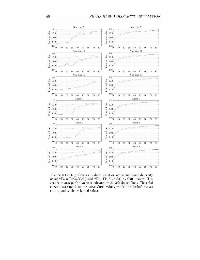
60 PHASE-BASED DISPARITY ESTIMATION
0 10 20 30 40 50 60 70 800.01
0.10 1.00 10.0 100
Err
or s
td. d
ev.
Non−ring 7
0 10 20 30 40 50 60 70 800.01
0.10 1.00 10.0 100
Err
or s
td. d
ev.
Non−ring 7
0 10 20 30 40 50 60 70 800.01
0.10 1.00 10.0 100
Err
or s
td. d
ev.
Non−ring 11
0 10 20 30 40 50 60 70 800.01
0.10 1.00 10.0 100
Err
or s
td. d
ev.
Non−ring 11
0 10 20 30 40 50 60 70 800.01
0.10 1.00 10.0 100
Err
or s
td. d
ev.
Non−ring 15
0 10 20 30 40 50 60 70 800.01
0.10 1.00 10.0 100
Err
or s
td. d
ev.
Non−ring 15
0 10 20 30 40 50 60 70 800.01
0.10 1.00 10.0 100
Err
or s
td. d
ev.
Gabor 1
0 10 20 30 40 50 60 70 800.01
0.10 1.00 10.0 100
Err
or s
td. d
ev.
Gabor 1
0 10 20 30 40 50 60 70 800.01
0.10 1.00 10.0 100
Err
or s
td. d
ev.
Gabor 2
0 10 20 30 40 50 60 70 800.01
0.10 1.00 10.0 100
Err
or s
td. d
ev.
Gabor 2
0 10 20 30 40 50 60 70 800.01
0.10 1.00 10.0 100
Err
or s
td. d
ev.
Gabor 3
0 10 20 30 40 50 60 70 800.01
0.10 1.00 10.0 100
Err
or s
td. d
ev.
Gabor 3
Figure 3.12: Log of error standard deviation versus maximum disparityusing \Twin Peaks"(left) and \Flip Flop" (right) as shift images. Thezero estimator performance is indicated with dash-dotted lines. The solidcurves correspond to the unweighted values, while the dashed curvescorrespond to the weighted values.

3.3 EXPERIMENTAL RESULTS 61
0 10 20 30 40 50 60 70 800.01
0.10 1.00 10.0 100
Err
or s
td. d
ev.
Lognorm 1
0 10 20 30 40 50 60 70 800.01
0.10 1.00 10.0 100
Err
or s
td. d
ev.
Lognorm 1
0 10 20 30 40 50 60 70 800.01
0.10 1.00 10.0 100
Err
or s
td. d
ev.
Lognorm 2a
0 10 20 30 40 50 60 70 800.01
0.10 1.00 10.0 100
Err
or s
td. d
ev.
Lognorm 2a
0 10 20 30 40 50 60 70 800.01
0.10 1.00 10.0 100
Err
or s
td. d
ev.
Lognorm 2b
0 10 20 30 40 50 60 70 800.01
0.10 1.00 10.0 100
Err
or s
td. d
ev.
Lognorm 2b
0 10 20 30 40 50 60 70 800.01
0.10 1.00 10.0 100
Err
or s
td. d
ev.
Lognorm 3a
0 10 20 30 40 50 60 70 800.01
0.10 1.00 10.0 100
Err
or s
td. d
ev.
Lognorm 3a
0 10 20 30 40 50 60 70 800.01
0.10 1.00 10.0 100
Err
or s
td. d
ev.
Lognorm 3b
0 10 20 30 40 50 60 70 800.01
0.10 1.00 10.0 100
Err
or s
td. d
ev.
Lognorm 3b
0 10 20 30 40 50 60 70 800.01
0.10 1.00 10.0 100
Err
or s
td. d
ev.
Lognorm 3c
0 10 20 30 40 50 60 70 800.01
0.10 1.00 10.0 100
Err
or s
td. d
ev.
Lognorm 3c
Figure 3.13: Log of error standard deviation versus maximum disparityusing \Twin Peaks"(left) and \Flip Flop" (right) as shift images. Thezero estimator performance is indicated with dash-dotted lines. The solidcurves correspond to the unweighted values, while the dashed curvescorrespond to the weighted values.

62 PHASE-BASED DISPARITY ESTIMATION
0 10 20 30 40 50 60 70 800.01
0.10 1.00 10.0 100
Err
or s
td. d
ev.
Windowed Fourier Transform 5
0 10 20 30 40 50 60 70 800.01
0.10 1.00 10.0 100
Err
or s
td. d
ev.
Windowed Fourier Transform 5
0 10 20 30 40 50 60 70 800.01
0.10 1.00 10.0 100
Err
or s
td. d
ev.
Windowed Fourier Transform 7
0 10 20 30 40 50 60 70 800.01
0.10 1.00 10.0 100
Err
or s
td. d
ev.
Windowed Fourier Transform 7
0 10 20 30 40 50 60 70 800.01
0.10 1.00 10.0 100
Err
or s
td. d
ev.
Windowed Fourier Transform 11
0 10 20 30 40 50 60 70 800.01
0.10 1.00 10.0 100
Err
or s
td. d
ev.
Windowed Fourier Transform 11
0 10 20 30 40 50 60 70 800.01
0.10 1.00 10.0 100
Err
or s
td. d
ev.
Binomial Gaussian differences
0 10 20 30 40 50 60 70 800.01
0.10 1.00 10.0 100
Err
or s
td. d
ev.
Binomial Gaussian differences
Figure 3.14: Log of error standard deviation versus maximum disparityusing \Twin Peaks"(left) and \Flip Flop" (right) as shift images. Thezero estimator performance is indicated with dash-dotted lines. The solidcurves correspond to the unweighted values, while the dashed curvescorrespond to the weighted values.

3.3 EXPERIMENTAL RESULTS 63
Figure 3.15: A natural image used for testing the bene�ts of combin-ing results from line and grey level images. (courtesy to CVAP, RoyalInstitute of Technology, Stockholm.)
3.3.5 Combining line and grey level results
In order to see the bene�ts of using both grey level images and line imagesthe experiments in Subsection 3.3.3 where repeated using grey level imagesonly and line images only. However, the structure of the noise imageis not ideal for showing how the line images contribute to the overallperformance, since there are no extended lines or edges. Instead, a naturalimage, shown in Figure 3.15, is used as original image in the scheme inFigure 3.4 on page 48. Figure 3.16 shows the results from the lognorm3c�lter when a natural image is used. Each row shows output certainty, thedisparity estimate and the error image. The �rst row corresponds to usingboth grey and line images, the second to grey level images only, and thethird to line images only. Note how the combined results bene�ts fromboth the other results. Where the line images fails the grey level imagesucceeds and vice versa.
Figures 3.17, 3.18 and 3.19 show the curves corresponding to the test inSubsection 3.3.3 with the image in Figure 3.15 instead of the noise imagein Figure 3.5 on page 49. A general observation is that the minimum

64 PHASE-BASED DISPARITY ESTIMATION
Figure 3.16: Top: The output certainty, the disparity estimate and theerror image from using both grey level images and line images. Middle:The same using grey level image only. Bottom: The same using lineimage only. Note how the combined results bene�ts from both the otherresults. Where the line images fail the grey level images succeed and viceversa.

3.3 EXPERIMENTAL RESULTS 65
error levels are slightly higher using the natural image than when usingthe noise image. This is due to the spatial consistency operation thatspreads the estimates from edges with high certainty into areas with weakimage structure.
Figures 3.20, 3.21 and 3.22 show the error plots corresponding to usinggrey level images only. The results from using line images only are shownin Figures 3.23, 3.24 and 3.25. The di�erences might at a �rst glance lookminimal but it should be kept in mind that the curves depict statistics forthe full image and that the error can be large locally, cf. Figure 3.16.
To point out a few interesting results, compare the nonring7 curves in theleft columns of Figures 3.17, 3.20 and 3.23. When using three levels ofresolution, the error from the combined result is lower than for any of theother two. On the other hand, when the number of resolution levels ishigh enough the di�erence is very small. This might seem disappointing,but is due to the fact that \Twin Peaks" is an nice �eld without disconti-nuities. The results corresponding to the \Flip Flop" image show that formost of the �lters, combining grey level image and line image estimatesis preferable. In particular, the �lters with a low center frequency, e.g.nonring15 and lognorm3c, bene�t from combining the estimates.

66 PHASE-BASED DISPARITY ESTIMATION
1 2 3 4 5 60.01
0.10 1.00 10.0
Err
or s
td. d
ev.
Non−ring 7
1 2 3 4 5 6 1.0
10.0
Err
or s
td. d
ev.
Non−ring 7
1 2 3 4 5 60.01
0.10 1.00 10.0
Err
or s
td. d
ev.
Non−ring 11
1 2 3 4 5 6 1.0
10.0
Err
or s
td. d
ev.
Non−ring 11
1 2 3 4 5 60.01
0.10 1.00 10.0
Err
or s
td. d
ev.
Non−ring 15
1 2 3 4 5 6 1.0
10.0
Err
or s
td. d
ev.
Non−ring 15
1 2 3 4 5 60.01
0.10 1.00 10.0
Err
or s
td. d
ev.
Gabor 1
1 2 3 4 5 6 1.0
10.0
Err
or s
td. d
ev.
Gabor 1
1 2 3 4 5 60.01
0.10 1.00 10.0
Err
or s
td. d
ev.
Gabor 2
1 2 3 4 5 6 1.0
10.0
Err
or s
td. d
ev.
Gabor 2
1 2 3 4 5 60.01
0.10 1.00 10.0
Err
or s
td. d
ev.
Gabor 3
1 2 3 4 5 6 1.0
10.0
Err
or s
td. d
ev.
Gabor 3
Figure 3.17: Log of error standard deviation versus number of resolu-tion levels using both grey level and line images. \Twin Peaks"(left)and \Flip Flop" (right) are used as shift images with 10 pixels maximumdisparity. The zero estimator performance is indicated with dash-dottedlines. The solid curves correspond to the unweighted values, while thedashed curves correspond to the weighted values.
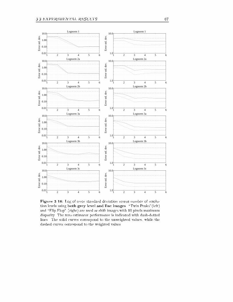
3.3 EXPERIMENTAL RESULTS 67
1 2 3 4 5 60.01
0.10 1.00 10.0
Err
or s
td. d
ev.
Lognorm 1
1 2 3 4 5 6 1.0
10.0
Err
or s
td. d
ev.
Lognorm 1
1 2 3 4 5 60.01
0.10 1.00 10.0
Err
or s
td. d
ev.
Lognorm 2a
1 2 3 4 5 6 1.0
10.0
Err
or s
td. d
ev.
Lognorm 2a
1 2 3 4 5 60.01
0.10 1.00 10.0
Err
or s
td. d
ev.
Lognorm 2b
1 2 3 4 5 6 1.0
10.0
Err
or s
td. d
ev.
Lognorm 2b
1 2 3 4 5 60.01
0.10 1.00 10.0
Err
or s
td. d
ev.
Lognorm 3a
1 2 3 4 5 6 1.0
10.0
Err
or s
td. d
ev.
Lognorm 3a
1 2 3 4 5 60.01
0.10 1.00 10.0
Err
or s
td. d
ev.
Lognorm 3b
1 2 3 4 5 6 1.0
10.0
Err
or s
td. d
ev.
Lognorm 3b
1 2 3 4 5 60.01
0.10 1.00 10.0
Err
or s
td. d
ev.
Lognorm 3c
1 2 3 4 5 6 1.0
10.0
Err
or s
td. d
ev.
Lognorm 3c
Figure 3.18: Log of error standard deviation versus number of resolu-tion levels using both grey level and line images. \Twin Peaks"(left)and \Flip Flop" (right) are used as shift images with 10 pixels maximumdisparity. The zero estimator performance is indicated with dash-dottedlines. The solid curves correspond to the unweighted values, while thedashed curves correspond to the weighted values.

68 PHASE-BASED DISPARITY ESTIMATION
1 2 3 4 5 60.01
0.10 1.00 10.0
Err
or s
td. d
ev.
Windowed Fourier Transform 5
1 2 3 4 5 6 1.0
10.0
Err
or s
td. d
ev.
Windowed Fourier Transform 5
1 2 3 4 5 60.01
0.10 1.00 10.0
Err
or s
td. d
ev.
Windowed Fourier Transform 7
1 2 3 4 5 6 1.0
10.0
Err
or s
td. d
ev.
Windowed Fourier Transform 7
1 2 3 4 5 60.01
0.10 1.00 10.0
Err
or s
td. d
ev.
Windowed Fourier Transform 11
1 2 3 4 5 6 1.0
10.0
Err
or s
td. d
ev.
Windowed Fourier Transform 11
1 2 3 4 5 60.01
0.10 1.00 10.0
Err
or s
td. d
ev.
Binomial Gaussian differences
1 2 3 4 5 6 1.0
10.0
Err
or s
td. d
ev.
Binomial Gaussian differences
Figure 3.19: Log of error standard deviation versus number of resolu-tion levels using both grey level and line images. \Twin Peaks"(left)and \Flip Flop" (right) are used as shift images with 10 pixels maximumdisparity. The zero estimator performance is indicated with dash-dottedlines. The solid curves correspond to the unweighted values, while thedashed curves correspond to the weighted values.

3.3 EXPERIMENTAL RESULTS 69
1 2 3 4 5 60.01
0.10 1.00 10.0
Err
or s
td. d
ev.
Non−ring 7
1 2 3 4 5 6 1.0
10.0
Err
or s
td. d
ev.
Non−ring 7
1 2 3 4 5 60.01
0.10 1.00 10.0
Err
or s
td. d
ev.
Non−ring 11
1 2 3 4 5 6 1.0
10.0
Err
or s
td. d
ev.
Non−ring 11
1 2 3 4 5 60.01
0.10 1.00 10.0
Err
or s
td. d
ev.
Non−ring 15
1 2 3 4 5 6 1.0
10.0
Err
or s
td. d
ev.
Non−ring 15
1 2 3 4 5 60.01
0.10 1.00 10.0
Err
or s
td. d
ev.
Gabor 1
1 2 3 4 5 6 1.0
10.0
Err
or s
td. d
ev.
Gabor 1
1 2 3 4 5 60.01
0.10 1.00 10.0
Err
or s
td. d
ev.
Gabor 2
1 2 3 4 5 6 1.0
10.0
Err
or s
td. d
ev.
Gabor 2
1 2 3 4 5 60.01
0.10 1.00 10.0
Err
or s
td. d
ev.
Gabor 3
1 2 3 4 5 6 1.0
10.0
Err
or s
td. d
ev.
Gabor 3
Figure 3.20: Log of error standard deviation versus number of resolu-tion levels using only grey level images. \Twin Peaks"(left) and \FlipFlop" (right) are used as shift images with 10 pixels maximum dispar-ity. The zero estimator performance is indicated with dash-dotted lines.The solid curves correspond to the unweighted values, while the dashedcurves correspond to the weighted values.

70 PHASE-BASED DISPARITY ESTIMATION
1 2 3 4 5 60.01
0.10 1.00 10.0
Err
or s
td. d
ev.
Lognorm 1
1 2 3 4 5 6 1.0
10.0
Err
or s
td. d
ev.
Lognorm 1
1 2 3 4 5 60.01
0.10 1.00 10.0
Err
or s
td. d
ev.
Lognorm 2a
1 2 3 4 5 6 1.0
10.0
Err
or s
td. d
ev.
Lognorm 2a
1 2 3 4 5 60.01
0.10 1.00 10.0
Err
or s
td. d
ev.
Lognorm 2b
1 2 3 4 5 6 1.0
10.0
Err
or s
td. d
ev.
Lognorm 2b
1 2 3 4 5 60.01
0.10 1.00 10.0
Err
or s
td. d
ev.
Lognorm 3a
1 2 3 4 5 6 1.0
10.0
Err
or s
td. d
ev.
Lognorm 3a
1 2 3 4 5 60.01
0.10 1.00 10.0
Err
or s
td. d
ev.
Lognorm 3b
1 2 3 4 5 6 1.0
10.0
Err
or s
td. d
ev.
Lognorm 3b
1 2 3 4 5 60.01
0.10 1.00 10.0
Err
or s
td. d
ev.
Lognorm 3c
1 2 3 4 5 6 1.0
10.0
Err
or s
td. d
ev.
Lognorm 3c
Figure 3.21: Log of error standard deviation versus number of resolu-tion levels using only grey level images. \Twin Peaks"(left) and \FlipFlop" (right) are used as shift images with 10 pixels maximum dispar-ity. The zero estimator performance is indicated with dash-dotted lines.The solid curves correspond to the unweighted values, while the dashedcurves correspond to the weighted values.

3.3 EXPERIMENTAL RESULTS 71
1 2 3 4 5 60.01
0.10 1.00 10.0
Err
or s
td. d
ev.
Windowed Fourier Transform 5
1 2 3 4 5 6 1.0
10.0
Err
or s
td. d
ev.
Windowed Fourier Transform 5
1 2 3 4 5 60.01
0.10 1.00 10.0
Err
or s
td. d
ev.
Windowed Fourier Transform 7
1 2 3 4 5 6 1.0
10.0
Err
or s
td. d
ev.
Windowed Fourier Transform 7
1 2 3 4 5 60.01
0.10 1.00 10.0
Err
or s
td. d
ev.
Windowed Fourier Transform 11
1 2 3 4 5 6 1.0
10.0
Err
or s
td. d
ev.
Windowed Fourier Transform 11
1 2 3 4 5 60.01
0.10 1.00 10.0
Err
or s
td. d
ev.
Binomial Gaussian differences
1 2 3 4 5 6 1.0
10.0
Err
or s
td. d
ev.
Binomial Gaussian differences
Figure 3.22: Log of error standard deviation versus number of resolu-tion levels using only grey level images. \Twin Peaks"(left) and \FlipFlop" (right) are used as shift images with 10 pixels maximum dispar-ity. The zero estimator performance is indicated with dash-dotted lines.The solid curves correspond to the unweighted values, while the dashedcurves correspond to the weighted values.

72 PHASE-BASED DISPARITY ESTIMATION
1 2 3 4 5 60.01
0.10 1.00 10.0
Err
or s
td. d
ev.
Non−ring 7
1 2 3 4 5 6 1.0
10.0
Err
or s
td. d
ev.
Non−ring 7
1 2 3 4 5 60.01
0.10 1.00 10.0
Err
or s
td. d
ev.
Non−ring 11
1 2 3 4 5 6 1.0
10.0
Err
or s
td. d
ev.
Non−ring 11
1 2 3 4 5 60.01
0.10 1.00 10.0
Err
or s
td. d
ev.
Non−ring 15
1 2 3 4 5 6 1.0
10.0
Err
or s
td. d
ev.
Non−ring 15
1 2 3 4 5 60.01
0.10 1.00 10.0
Err
or s
td. d
ev.
Gabor 1
1 2 3 4 5 6 1.0
10.0
Err
or s
td. d
ev.
Gabor 1
1 2 3 4 5 60.01
0.10 1.00 10.0
Err
or s
td. d
ev.
Gabor 2
1 2 3 4 5 6 1.0
10.0
Err
or s
td. d
ev.
Gabor 2
1 2 3 4 5 60.01
0.10 1.00 10.0
Err
or s
td. d
ev.
Gabor 3
1 2 3 4 5 6 1.0
10.0
Err
or s
td. d
ev.
Gabor 3
Figure 3.23: Log of error standard deviation versus number of reso-lution levels using only line images. \Twin Peaks"(left) and \FlipFlop" (right) are used as shift images with 10 pixels maximum dispar-ity. The zero estimator performance is indicated with dash-dotted lines.The solid curves correspond to the unweighted values, while the dashedcurves correspond to the weighted values.

3.3 EXPERIMENTAL RESULTS 73
1 2 3 4 5 60.01
0.10 1.00 10.0
Err
or s
td. d
ev.
Lognorm 1
1 2 3 4 5 6 1.0
10.0
Err
or s
td. d
ev.
Lognorm 1
1 2 3 4 5 60.01
0.10 1.00 10.0
Err
or s
td. d
ev.
Lognorm 2a
1 2 3 4 5 6 1.0
10.0
Err
or s
td. d
ev.
Lognorm 2a
1 2 3 4 5 60.01
0.10 1.00 10.0
Err
or s
td. d
ev.
Lognorm 2b
1 2 3 4 5 6 1.0
10.0
Err
or s
td. d
ev.
Lognorm 2b
1 2 3 4 5 60.01
0.10 1.00 10.0
Err
or s
td. d
ev.
Lognorm 3a
1 2 3 4 5 6 1.0
10.0
Err
or s
td. d
ev.
Lognorm 3a
1 2 3 4 5 60.01
0.10 1.00 10.0
Err
or s
td. d
ev.
Lognorm 3b
1 2 3 4 5 6 1.0
10.0
Err
or s
td. d
ev.
Lognorm 3b
1 2 3 4 5 60.01
0.10 1.00 10.0
Err
or s
td. d
ev.
Lognorm 3c
1 2 3 4 5 6 1.0
10.0
Err
or s
td. d
ev.
Lognorm 3c
Figure 3.24: Log of error standard deviation versus number of reso-lution levels using only line images. \Twin Peaks"(left) and \FlipFlop" (right) are used as shift images with 10 pixels maximum dispar-ity. The zero estimator performance is indicated with dash-dotted lines.The solid curves correspond to the unweighted values, while the dashedcurves correspond to the weighted values.

74 PHASE-BASED DISPARITY ESTIMATION
1 2 3 4 5 60.01
0.10 1.00 10.0
Err
or s
td. d
ev.
Windowed Fourier Transform 5
1 2 3 4 5 6 1.0
10.0
Err
or s
td. d
ev.
Windowed Fourier Transform 5
1 2 3 4 5 60.01
0.10 1.00 10.0
Err
or s
td. d
ev.
Windowed Fourier Transform 7
1 2 3 4 5 6 1.0
10.0
Err
or s
td. d
ev.
Windowed Fourier Transform 7
1 2 3 4 5 60.01
0.10 1.00 10.0
Err
or s
td. d
ev.
Windowed Fourier Transform 11
1 2 3 4 5 6 1.0
10.0
Err
or s
td. d
ev.
Windowed Fourier Transform 11
1 2 3 4 5 60.01
0.10 1.00 10.0
Err
or s
td. d
ev.
Binomial Gaussian differences
1 2 3 4 5 6 1.0
10.0
Err
or s
td. d
ev.
Binomial Gaussian differences
Figure 3.25: Log of error standard deviation versus number of reso-lution levels using only line images. \Twin Peaks"(left) and \FlipFlop" (right) are used as shift images with 10 pixels maximum dispar-ity. The zero estimator performance is indicated with dash-dotted lines.The solid curves correspond to the unweighted values, while the dashedcurves correspond to the weighted values.
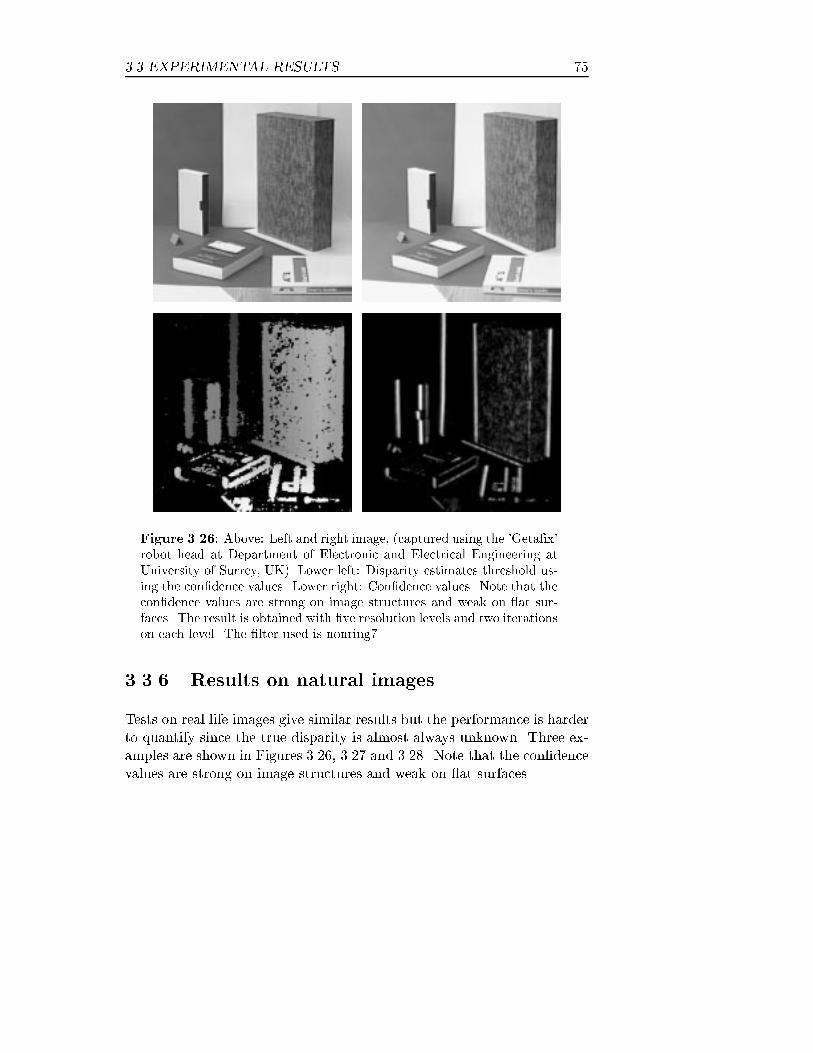
3.3 EXPERIMENTAL RESULTS 75
Figure 3.26: Above: Left and right image, (captured using the 'Geta�x'robot head at Department of Electronic and Electrical Engineering atUniversity of Surrey, UK). Lower left: Disparity estimates threshold us-ing the con�dence values. Lower right: Con�dence values. Note that thecon�dence values are strong on image structures and weak on at sur-faces. The result is obtained with �ve resolution levels and two iterationson each level. The �lter used is nonring7.
3.3.6 Results on natural images
Tests on real life images give similar results but the performance is harderto quantify since the true disparity is almost always unknown. Three ex-amples are shown in Figures 3.26, 3.27 and 3.28. Note that the con�dencevalues are strong on image structures and weak on at surfaces.

76 PHASE-BASED DISPARITY ESTIMATION
Figure 3.27: Above: Left and right image, (captured using the 'Geta�x'robot head at Department of Electronic and Electrical Engineering atUniversity of Surrey, UK). Lower left: Disparity estimates threshold us-ing the con�dence values. Lower right: Con�dence values. Note that thecon�dence values are strong on image structures and weak on at sur-
faces. The result is obtained with �ve resolution levels and two iterationson each level. The �lter used is nonring7.

3.3 EXPERIMENTAL RESULTS 77
Figure 3.28: Two images from the Sarno� tree sequence. Above: Leftand right image. Lower left: Disparity estimates threshold using the con-�dence values. Lower right: Con�dence values. Note that the con�dencevalues are strong on image structures and weak on at surfaces. Theresult is obtained with four resolution levels and two iterations on eachlevel. The �lter used is nonring7.

78 PHASE-BASED DISPARITY ESTIMATION
3.4 Conclusion
The test results show that the overall performance of the stereo algorithmis not critically dependent on the type of disparity �lter used. The con-sistency checks and edge image �ltering applied in order to enhance theperformance of the algorithm, do indeed reduce the impact of the actual�lter shape.
There are, however, some conclusions to be made. The results of the phasebased stereo algorithm in Section 3.3, are somewhat contradictory to theresults of the investigation of the singular points in Section 2.3. The stereotests indicate that �lters with a wide bandwidth are preferable, while anarrow bandwidth is more advantageous from a phase scale space pointof view. The reason is that broad band �lters have less phase cyclesand therefore can handle greater disparities for a given �lter size. Thecomputational e�ciency that follows from this implies that the best �lterchoice is the �lters without wrap around; Di�erence-of-Gaussians are verysmall and thus requires more levels of resolution, while the non-ringing�lters are larger and manages with a smaller number of levels. As pointedout earlier, it is not always possible to compensate small size with byincreasing the number of levels.
The poor performance of the WFT �lters is due to the rectangular win-dow. Such a window gives image structures in the �lter periphery thesame importance as one close to the �lter center. The frequency domainrepresentation of the �lters show that they are sensitive to high-frequencynoise due to the long tails of ripples (Figure 2.14 on page 30). As men-tioned before, Weng suggests a low pass pre�ltering of the input image[71]. The resulting �lter is very close to the nonring �lters and so are thecorresponding results. The reason for using the non-pre�ltered version ofWFT here is to show that the pre�ltering is not a little adjustment to getrid of little noise; it is crucial for the operation to work.

3.5 FURTHER RESEARCH 79
3.5 Further research
The problem with �lter interference mentioned in Subsection 3.3.3 can bereduced by introducing a correlation stage in the computational structure.A correlation stage means that instead of computing phase di�erencespointwise only, it is done over a neighborhood, and the di�erence valuewith the highest con�dence is used as disparity estimate. On a certainlevel, disparities larger that the �lter support can be captured. Largerdisparities can then be estimated for a given �lter and a given number ofresolution levels. The computational cost is of course higher, especially ifthe correlation neighborhood is large. A compromise is to use correlationat the coarsest resolution only, since correct estimates there reduces thedisparities at lower levels [30, 31].
All real stereo pairs have more or less vertical disparities as well as hori-zontal, due to camera geometry etc. To be able to handle general cases,further work will include extending the algorithm to two dimensions, es-timating vertical disparities as well. This can be implemented either byinterleaving two one-dimensional algorithms, one horizontal and one ver-tical, or by using two-dimensional �lters in the disparity estimator. Amethod for two-dimensional disparities based on the phase in the Multires-olution Fourier Transform, MFT, has been developed by Calway, Knutssonand Wilson [17, 16].
Being able to handle multiple disparities in the same image point is alsoa potentially useful extension. See for instance [70] for a multiple motionapproach to motion estimation.

80 PHASE-BASED DISPARITY ESTIMATION
4HIERARCHICAL DATA-DRIVEN
FOCUS OF ATTENTION
4.1 Introduction
A fundamental problem yet to be solved in computer vision in generaland active vision in particular is that of how to focus the attention of asystem. The issues involved in focus of attention (FOA) incorporate notonly where to look next but also more abstract mechanisms such as howto concentrate on certain features in the continuous ow of input data.
There are several reasons for narrowing the channel of input informationby focusing on speci�c parts. The most obvious reason for FOA is toreduce the vast amount of input data to match the available computationalresources. However, the ability to decompose a complex problem intosimpler subproblems has also been put forward as a major motivation forusing focus of attention mechanisms.
4.1.1 Human focus of attention
Humans can shift the attention either by moving the �xation point or byconcentrating on a part of the �eld of view. The two types are called overtand covert attention respectively. The covert attention shifts are aboutfour times as fast as the overt shifts. This speed di�erence can be used tocheck a potential �xation point to see if it is worthwhile moving the gazeto that position.
81

82 HIERARCHICAL DATA-DRIVEN FOCUS OF ATTENTION
A number of paradigms describing human focus of attention has beendeveloped over the years [57]. In the zoom-lens metaphor computationalresources can either be spread on the whole �eld of view, 'wide angle lens',or concentrated on a portion, 'telephoto lens'. This metaphor is foundedon the assumption that the computational resources are the main causefor having to focus the attention on one thing at the time. Thus, theproblem is to allocate the available resources properly.
The work presented below relates to the search light metaphor [41]. Abasic assumption in this metaphor is the division between preattentiveand attentive perception. The idea is that the preattentive part of thesystem makes a crude analysis of the �eld of view. The attentive part thenanalyzes areas indicated as being particularly interesting more closely.The two systems should not be seen as taking turns in a time multiplexmanner, but rather as a pipeline where the attentive part makes selectiveuse of the continuous stream of results from the preattentive part. Theterm 'search light' re ects how the attentive system analyzes parts of theinformation available by illuminating it with an attentional search light.The reason for having to focus the attention in this metaphor is that sometasks are inherently of sequential nature.
What features or properties are then important for positioning the �xationpoint? For attentional shifts the criterion is closely connected to the taskat hand. Yarbus pioneered the work on studying how human move the�xation point in images depending on the wanted information [88]. Forpre-attentional shifts gradients in space and time, i.e high contrast areasor motion, are considered to be the important features. Abbott and Ahujapresent a list of criteria for the choice of the next �xation point [1]. Manyof the items in the list relate to computational considerations concerningthe surface reconstruction algorithm presented. However, a few clues fromhuman visual behavior was also included:
Absolute distance and direction. If multiple candidates for �xationpoints are present, the ones closer to the center of the viewing �eldare more likely to be chosen. Upward movement is generally pre-ferred to downward movement.
4.1 INTRODUCTION 83
2D images characteristics. If polygonal objects are presented, pointsclose to corners are likely to be chosen as �xation points. Whensymmetries are present, the �xation point tends to be chosen alongsymmetry lines.
Temporal changes. When peripheral stimuli suddenly appear, a strongtemporal cue often leads to a movement of �xation point towardsthe stimuli.
Since �xation point selection is a highly task dependent action, it is proba-bly easy to construct situations that contradict the list above. The readeris urged to consult for the appropriate references in order to get a fulldescription of how the results were obtained.
4.1.2 Machine focus of attention
A number of research groups are currently working on incorporating focusof attention mechanisms in computer vision algorithms. This section is byno means a comprehensive overview, but rather presents a few interestingexamples.
The Vision as Process consortium, ESPRIT Basic Research Action 3038and 7108, was united by the scienti�c hypothesis that vision should bestudied as a continuous process. The project is aimed at bringing to-gether knowhow from a wide variety of research �elds ranging low levelfeature extraction and ocular re exes through object recognition and taskplanning [69, 22].
Ballard and Brown have produced a series of experiments with ocularre exes and visual skills [6, 11, 13, 12, 7]. The basic idea is to use simpleand fast image processing algorithms in combination with a exible, activeperceiving system.
A focus of attention system based on salient features has been developedby Milanese [58]. A number of features are extracted from the input imageand are represented in a set of feature maps. Features di�ering from their

84 HIERARCHICAL DATA-DRIVEN FOCUS OF ATTENTION
surroundings are moved to a corresponding set of conspicuity maps. Thesemaps consist of interesting regions of each feature. The conspicuity mapsare then merged into a central saliency map where the attention systemgenerates a sequence of attention shifts based on the activity in the map.
Brunnstr�om, Eklund and Lindeberg have presented an active vision ap-proach to classifying corner points in order to examine the structure of thescene. Interesting areas are detected and potential corner points scruti-nized by zooming in on them [15, 14]. The possibility of actively choosingthe imaging parameters, e.g. point of view and focal length, allows theclassi�cation algorithm to be much simpler than for static images or pre-recorded sequences.
A variation of the search light metaphor, called the attentional beamhas been developed by Tsotsos and Culhane [23, 66, 67]. It is basedon a hierarchical information representation where a search light on thetop is passed downwards in the hierarchy to all processing units thatcontribute to the attended unit. Neighboring units are inhibited. Theinformation in the 'beamed' part of the hierarchy is reprocessed, withoutthe interference from the neighbors, the beam is then used to inhibit theprocessing elements and a new beam is chosen.
4.2 Space-variant sampled image sensors: Foveas
4.2.1 What is a fovea?
Space-variant image sampling is not strictly necessary for studying focus ofattention and gaze control, but the need for positioning the �xation pointis more evident for such a sensor. There are, however, compelling biolog-ical and technical reasons for exploring the use of space-variant sampledsensors.
The human eye has its highest resolution in the center and decays towardthe periphery. The �rst 15� it decays linearly with the angle to the optic

4.2 SPACE-VARIANT SAMPLED IMAGE SENSORS: FOVEAS 85
axis, then the reduction is even faster. The center part is called thefovea and has a visual �eld of about 1:75�. This corresponds to about 45millimeters 1.5 meters away. As a comparison, the total visual �eld usingboth eyes is about 180� [38]. There are a number of advantages in suchan arrangement, for example:
� Data reduction compared to having the whole �eld of view in fullresolution.
� High resolution is combined with a broad �eld of view.
� The e�ects of image warping due to wide angle lens distortion isreduced. The distortion increases with the angle from the opticaxis, but the resolution decreases.
� The periphery vision gathers information about other possible pointsof interest, and of contextual in uence. Therefore, the processing inthis area does not have to be so comprehensive.
These advantages can be utilized in a robot vision system as well. Thereare a number of research projects developing both hardware and algo-rithms for space-variant sampled image arrays, all exemplifying imple-mentations of the fovea concept [65, 64, 68].
In human vision fovea refers to the central part of the retina, but in robotvision the term is often used to indicate that the system treats the centraland the peripheral parts of the �eld of view di�erently.
4.2.2 Creating a log-Cartesian fovea
The log-Cartesian fovea representation of the �eld of view is a central partof the system presented in this thesis, and it can be seen as a special caseof a subsampled resolution pyramid. The di�erence is that it is only thecenter part that is represented in all resolutions, or scales (Figure 4.1 onthe following page).

86 HIERARCHICAL DATA-DRIVEN FOCUS OF ATTENTION
Figure 4.1: Upper left: Original image. The skewed appearance is dueto the broad �eld of view, 90�. Upper right: Low Pass pyramid. Lowerleft: Center part of each level in the pyramid. Lower right: Interpolatedcenter part images stacked on top of each other. The borders betweenthe levels are marked for clarity.

4.2 SPACE-VARIANT SAMPLED IMAGE SENSORS: FOVEAS 87
Figure 4.2: Topmost left: The original 512� 512 image. The following�ve 32�32 images are the log-Cartesian fovea representation. The levelscorrespond to the visual angles 90�, 53�, 28�, 14� and 7� respectively.The levels are numbered from 0 to 4 where 0 corresponds to the �nestresolution.
88 HIERARCHICAL DATA-DRIVEN FOCUS OF ATTENTION
In the system presented here the log-Cartesian fovea is generated by re-peated LP-�ltering, subsampling and cropping in octaves. The input im-age is LP-�ltered with a Gaussian (� = 4=� [36]) which allows subsam-pling by a factor two. The new image then has the same �eld of view buthalf the number of pixels in each direction. The subsampling procedureis repeated until the desired number of levels is reached. This generatesa subsampled resolution pyramid of the same �eld of view but di�erentsize on each level. All levels are then cropped to the same size by keepingthe center parts and discarding the rest. The result is a number of levelswith the same number of pixels but with di�erent resolution, i.e. coveringdi�erent �elds of view. In a real system it would be preferable to have anoptic system that generates the fovea as the input images are digitized.
Figure 4.1 shows an example starting with a 512 � 512 image and using5 levels. LP-�ltering and subsampling four times reduces the size of the�nal level to 32� 32 pixels. Cutting out the center 32� 32 pixels at eachlevel reduces the data by a factor 512�512
5�32�32 = 51:2. Figure 4.2 on the pagebefore shows the individual images in the fovea representation. The lowerright image in Figure 4.1 shows the total �eld of view which is visualizedby interpolating and combining the images.
Note that although the fovea representation is often visualized as one im-age with varying resolution, it is actually N separate images with di�erentresolution. The levels are numbered from 0 to N �1, where 0 correspondsto the highest resolution.

4.2 SEQUENTIALLY DEFINED, DATA MODIFIED FOA 89
4.2.3 Image operations in a fovea
The image operations that are used are applied on all levels of resolution.Figure 4.3 on the following page illustrates two di�erent ways of handlingthe part of a �lter that reaches outside the image. The image is the�nest resolution part of the fovea representation in Figure 4.2 on page 87.When convolving an image with a �lter, it is common to pad the image byrepeating the border pixels as far as the �lter reaches outside the image asin the upper left image of Figure 4.3. Note how the texture is expandedinto linear structures to the right and below the image. Also note howthe lower right corner pixel turns into a large square. On images muchlarger than the �lter this distortion is often acceptable since it is onlya small portion of the total image. In a fovea representation, however,the images are only a few times larger than the �lters. Especially whenusing successive �ltering this becomes a problem, since the border e�ectsspread, and eventually dominate the results.
When �ltering a particular level in a fovea representation, that level canbe padded with information from the nearest coarser level, which covers alarger neighborhood but with lower resolution, (lower left in Figure 4.3).This means that it is possible to get a better border by interpolating thecorresponding area in the nearest coarser level. The unwanted border ef-fects that otherwise might disturb the algorithms are then reduced. Note,for instance, that the cube appears to be much larger when border exten-sion is used. This does not happen if the information instead is pickedfrom the nearest coarser level, (lower right in Figure 4.3).
4.3 Sequentially de�ned, data modi�ed focus of
attention
4.3.1 Control mechanism components
Having full resolution only in the center part of the visual �eld makes itobvious that a good algorithm for positioning the �xation point is neces-

90 HIERARCHICAL DATA-DRIVEN FOCUS OF ATTENTION
Figure 4.3: Upper left: One level in a fovea. Upper right: Paddingby copying border pixels. Note how the texture is expanded into linearstructures to the right and below the image. Also note how the lowerright corner pixel turns into a big square. Lower left: Next coarser levelgives information about a larger neighborhood around the same point,but with lower resolution. Lower right: Using interpolated informationfrom the coarser level to pad the image. The interpolated information ismore coherent with the real neighborhood than the extended border.
sary. A number of focus-of-attention control mechanisms must be activesimultaneously to be able to both handle unexpected events and performan e�ective search. The di�erent components can roughly be divided intothe following groups:

4.3 SEQUENTIALLY DEFINED, DATA MODIFIED FOA 91
1. Preattentive, data driven control. Non-predicted structured imageinformation and events attract the focus-of-attention in order to getthe information analyzed.
2. Attentive, model driven control. The focus-of-attention is directedtoward an interesting region according to predictions using alreadyacquired image information or apriori knowledge.
3. Habituation. As image structures are analyzed and modeled theirimpact on preattentive gaze control is reduced.
The distinction between the preattentive and attentive parts is oating.It is more of a spectrum from pure re exes to pure attentional movementsof the �xation point.
4.3.2 The concept of nested regions of interest
In the hierarchical system shown in Figure 1.2 all levels might have anidea about how to position the camera in order to solve their own currentproblems. One way of solving this is to let the di�erent levels take turnsin controlling the camera. Another way is to recognize the fact that theinteresting area for a level is often a sub-area of the interesting area of thelevel above. Moreover, the task of a level is often directly related to thetask of the level above. Positioning the �xation point can therefore be are�nement from coarse to �ne, where higher levels give the major regionof interest and lower levels adjust to interesting areas within that region.Consider the following stylized example:
Assume there are the following four major levels, from top to bottom, inthe information processing hierarchy on the left hand side of the pyramid(the names are borrowed from the Esprit project BRA 3038, Vision asProcess):
1. System Supervisor
2. Symbolic Scene Interpreter
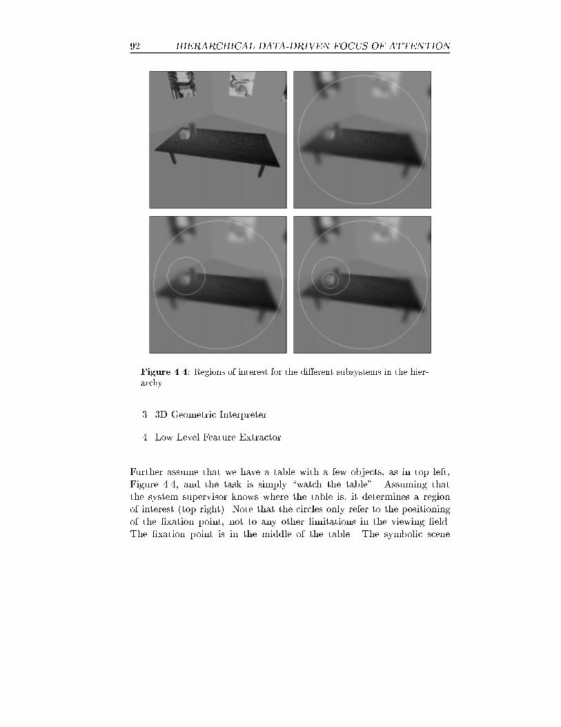
92 HIERARCHICAL DATA-DRIVEN FOCUS OF ATTENTION
Figure 4.4: Regions of interest for the di�erent subsystems in the hier-archy.
3. 3D Geometric Interpreter
4. Low Level Feature Extractor
Further assume that we have a table with a few objects, as in top left,Figure 4.4, and the task is simply \watch the table". Assuming thatthe system supervisor knows where the table is, it determines a regionof interest (top right). Note that the circles only refer to the positioningof the �xation point, not to any other limitations in the viewing �eld.The �xation point is in the middle of the table. The symbolic scene

4.3 SEQUENTIALLY DEFINED, DATA MODIFIED FOA 93
interpretor has found indications of an object or group of objects in theupper left corner of the table and sets its region of interest accordingly(lower left). The 3D Geometric Interpreter starts its task by a furtherre�nement of the region of interest by marking the bright object (lowerright). Finally, on the lowest level, the Low Level Feature Extractor selectsan area to start model the structures in the image. The �xation point isnow moved towards the interesting object by the nested regions of interest.The general response command \watch the table" has been transformedinto \focus on the set of objects in the upper left corner of the table".
The border of the regions of interest are not to be absolute, rigid bound-aries. They are rather recommendations that can be neglected if there aregood reasons. How good a reason must be is controlled with an impor-tance value. This can be illustrated by viewing the region of interest asa basin, or potential well, within which the lower levels can move aroundfreely. The slope and height of the wall is proportional to how importantit is to keep the �xation point there.
There are, however, situations when the lower levels are supposed to vi-olate the directives from superior levels. One such occasion is event de-tection. Here, an event is an unpredicted gradient in space and/or time.When an interesting or important stimuli is detected, the �xation pointshould be moved in that direction on a re ex basis. Suppose the systemis watching the table and an object enters the scene and is detected in the'corner of the eye'. The resolution in the periphery is probably not highenough to see what it is, only where it is. The low level feature extractoris the �rst level to detect the event and reacts by pulling the �xation pointtowards the event. By the time the higher levels react on the event thereare extracted low level features with high resolution available. The higherlevels will now either move their regions of interest to analyze the eventfurther or force the �xation point back to the original position. Thus,the di�erent regions of interest do not have to be determined in the orderindicated in Figure 4.4. It all depends on whether it is an attentive orpreattentive movement of the �xation point.

94 HIERARCHICAL DATA-DRIVEN FOCUS OF ATTENTION
Figure 4.5: The robot con�guration. The robot is a Puma 560 arm withsix degrees of freedom equipped with a head with two movable cameraswith one degree of freedom each; the camera pan angle.
4.4 Gaze control
4.4.1 System description
In the experiments below the robot consists of an arm with a camerahead, (Figure 4.5). The robot is a Puma 560 arm with six degrees offreedom. In the experiments presented here only two degrees of freedomare used. They implement head pan and head tilt angles. The head hastwo movable cameras with one degree of freedom each; the camera panangle. The purpose of this system might be automatic identi�cation, in-spection or even surveillance of the objects in the scene in front of it. Thistype of robotic vision system is wide-spread, see for instance [1, 11, 21].The system, both image generation and analysis, is implemented in theApplication Visualisation System, AVS, which is described in Chapter 6.
4.4 GAZE CONTROL 95
The cameras are equipped with log-Cartesian sensors. The total �eld ofview is 90� and the fovea consists of 5 levels. The individual �elds of vieware in the experiments 7�, 14�, 28�, 53� and 90� respectively.
The outward response of this particular system is designed to enable in-formation gathering. Interesting events in the �eld of view attract the�xation point in order to get them within the high resolution part of thefovea. The robot does not move objects. In this experiments it is onlypermitted to change the point of view using the head pan and tilt, andcamera vergence.
The robot has a gaze control system with three levels (Figure 4.6). Thetop level is an object detector, or rather a symmetry detector [9, 37, 82],drawing the attention towards regions of high complexity. The secondlevel is a line tracker drawing the �xation point towards, and along, linearstructures based on local orientation and phase [44, 75, 76]. The lowestlevel verges the cameras to make them have the same �xation point usingthe disparity estimates from the stereo algorithm described in Chapter 3.
4.4.2 Control hierarchy
The left hand side of Figure 4.6 shows the feature hierarchy with increasingabstraction going upwards. More abstract features are stepwise composedfrom simpler ones. The features are used both as ground for more complexfeatures and as modi�ers for response outputs. The right hand side of thesame �gure shows the response hierarchy with increasing speci�city goingdownwards [33, 72]. The re�nement of the positioning of the �xation pointis handled with potential �elds in the robot's parameter space [52]. It canbe visualized as an 'energy landscape', as in Figure 4.10 on page 103,where the �xation point trajectory is the path a little ball freely rollingaround would take. The �xation point can be moved to a certain positionby forming a potential well around the position in the parameter spacecausing to the robot to look in that direction.

96 HIERARCHICAL DATA-DRIVEN FOCUS OF ATTENTION
CAMERA INPUTS CAMERA CTRL
HEAD CTRL
STEREO
VERGENCEFOVEA
ORIENT
"OBJECT FINDER"
"EDGE TRACKER"
HEAD CTRL
ROTCONS
2D PHASE
DISTMASS
Figure 4.6: The preattentive focus of attention system.
4.4.3 Disparity estimation and camera vergence
The lowest level in the control system is the camera vergence process.The cameras are verged symmetrically to get zero disparity in the centerof the image regardless of the state of the system. If the head is movingthe vergence is calculated using the disparity from the part of the �eld ofview that is predicted to be centered in the next time step.
The disparity is measured using the multi-scale method based on the phasein quadrature �lters described in Chapter 3. The fovea version has twomajor di�erences compared to the computation structure in Figure 3.2 onpage 39. First, only the center of the �eld of view is represented in allresolutions. The accuracy of disparity estimates therefore decays towardsthe periphery of the �eld of view. Second, the edge extractor is used on

4.4 GAZE CONTROL 97
α
Figure 4.7: Vector representation of local orientation.
every level of the input pyramid, instead of creating a pyramid from theedge representation of the �nest resolution. This di�erence is motivatedby a possible future fovea sensor array. In such a system it would not bepossible to have the computational structure in Figure 3.2, since a highresolution image of the total �eld of view does not exist.
4.4.4 The edge tracker
Apart from estimating disparity, the phase from quadrature �lters is alsoused to generate a potential �eld drawing the attention towards and alonglines and edges in the image [75]. This is the second level in the controlstructure in Figure 4.6.
Local orientation
An algorithm for phase-invariant orientation estimation in two dimensionsis presented in [44]. Phase-invariant means that the orientation of a locallyone-dimensional signal can be estimated regardless of it being an edgeor a line, i.e. regardless of the phase. The orientation is represented asa complex number, where the argument represents the local orientationestimate and the magnitude indicates the certainty of the estimate [32].

98 HIERARCHICAL DATA-DRIVEN FOCUS OF ATTENTION
Figure 4.7 shows the correspondence between the complex number andthe local orientation. Note that the argument varies twice as fast as theorientation of the local structure:
z =Mei� =Mei2' (4.1)
where ' is the the angle between the gradient and the horizontal axis.Rotating a line � radians makes it look the same as the initial line whichmeans that the representation has to be the same. The key feature of thisrepresentation is that maximally incompatible orientations are mappedon complex numbers with opposite signs. This, in turn, makes averaginga meaningful operation.
When working with resolution pyramids, information is LP �ltered andsubsampled, interpolated etc. The information representation has to becontinuous in order for these operations to give meaningful results. If theaverage of the representations of the structure in two points represents astructure that is completely di�erent, then the representation is not usefulin a resolution pyramid.
Representation of phase in higher dimensions
In Chapter 2 only one-dimensional signals are discussed. The extensionof the phase concept into two or more dimensions is not trivial [36]. InSection 2.1 it is shown that the local phase is connected to the analyticfunction and hence to the Hilbert transform. A direction of reference hasto be introduced in order to make a multi-dimensional de�nition of theHilbert transform possible. Thus, local phase needs a direction of referenceas well.
If a continuous representation is desired, the phase cannot be representedwith only a single value, although it is a scalar. The phase representationhas to include both the phase value and the reference direction. Thismeans in the general case that if the dimensionality of the signal space isN, the dimensionality of the phase representation is N+1 [34].
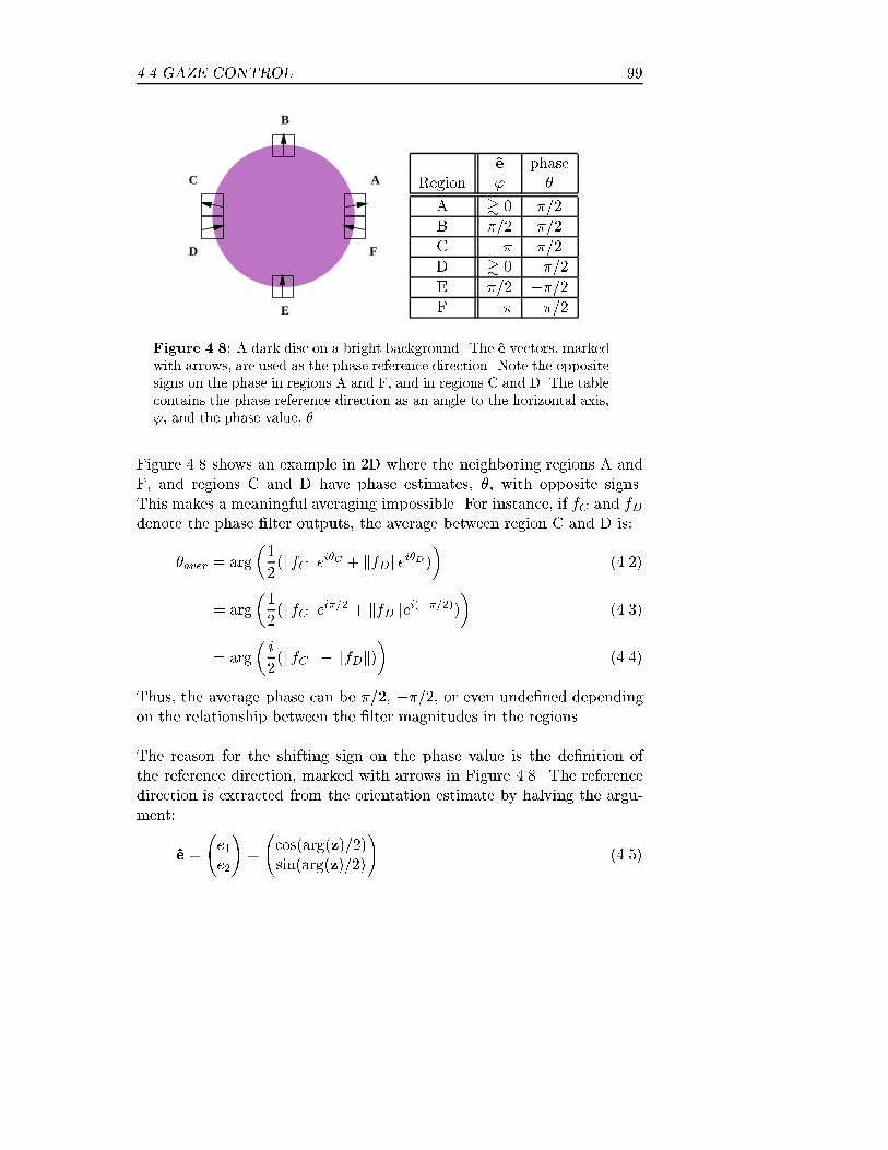
4.4 GAZE CONTROL 99
B
AC
D F
E
e phaseRegion ' �
A & 0 �=2
B �=2 �=2
C . � �=2
D & 0 ��=2E �=2 ��=2F . � ��=2
Figure 4.8: A dark disc on a bright background. The e vectors, markedwith arrows, are used as the phase reference direction. Note the oppositesigns on the phase in regions A and F, and in regions C and D. The tablecontains the phase reference direction as an angle to the horizontal axis,', and the phase value, �.
Figure 4.8 shows an example in 2D where the neighboring regions A andF, and regions C and D have phase estimates, �, with opposite signs.This makes a meaningful averaging impossible. For instance, if fC and fDdenote the phase �lter outputs, the average between region C and D is:
�aver = arg
�1
2(kfCkei�C + kfDkei�D )
�(4.2)
= arg
�1
2(kfCkei�=2 + kfDkei(��=2))
�(4.3)
= arg
�i
2(kfCk � kfDk)
�(4.4)
Thus, the average phase can be �=2, ��=2, or even unde�ned dependingon the relationship between the �lter magnitudes in the regions.
The reason for the shifting sign on the phase value is the de�nition ofthe reference direction, marked with arrows in Figure 4.8. The referencedirection is extracted from the orientation estimate by halving the argu-ment:
e =
e1e2
!=
cos(arg(z)=2)sin(arg(z)=2)
!(4.5)
100 HIERARCHICAL DATA-DRIVEN FOCUS OF ATTENTION
Since the phase is measured along e, it will change sign if e changes to theopposite direction. Two neighboring points may have e in opposite direc-tions and thus phase values with opposite signs, although they belong tothe same image structure. Averaging of such a neighborhood would there-fore be meaningless. It can be argued that choosing the phase referencedirections such that they all point out from the object solves the problem,but it is impossible to locally determine what is the inside or the outsideof an object. With only local information available, region A could forinstance be a region F on a white disc on a dark background.
A 2D-phase representation, suggested by Knutsson, that includes the ref-erence direction in a two-dimensional space is:
x =
0B@x1x2x3
1CA =
0B@M cos(') sin(�)M sin(') sin(�)
M cos(�)
1CA (4.6)
where
M 2 [0;1] is the signal energy,' 2 [0; �] is the reference direction, and� 2 [��; �] is the phase value.
Resolving the phase angle, �, gives:
� = arctan
�qx21 + x22; x3
�(4.7)
Figure 4.9 shows the representation which can be interpreted as a 3Dvector of length M rotated an angle � in a plane de�ned by e and x3.The shaded circle corresponds to the phase representation in 1D shownin Figure 2.3 on page 9. An intuitive feeling for how this representationsolves the problem in the example above can be obtained by some mentalimaging. Turn e around x3 until it points in the opposite direction. Thephase value, �, is then de�ned in the opposite direction. In other words,when the reference direction changes sign the phase angle de�nition alsochanges sign.

4.4 GAZE CONTROL 101
θ
ϕ
x3
e
M
1x
2x
Figure 4.9: A 3D representation of phase in 2D.
The phase estimate in region C in Figure 4.8 on page 99 is now:
xC =
0B@MC cos(�) sin(�=2)MC sin(�) sin(�=2)
MC cos(�=2)
1CA =
0B@�MC
0:00:0
1CA (4.8)
and in region D it is:
xD =
0B@MD cos(0) sin(��=2)MD sin(0) sin(��=2)MD cos(��=2)
1CA =
0B@�MD
0:00:0
1CA (4.9)
The average phase in a neighborhood is simply the average of the compo-nents, xi, respectively:
xaver =
0B@
12(x1C + x1D)
12(x2C + x2D)
12(x3C + x3D)
1CA =
0B@
12((�MC) + (�MD))
0:00:0
1CA (4.10)
Note that the direction of the average phase vector is now independent ofthe signal energy in the two �lter as opposed to the case in Equation (4.2).

102 HIERARCHICAL DATA-DRIVEN FOCUS OF ATTENTION
The average phase angle, �aver, can be calculated using Equation (4.7):
�aver = arctan
� 12(MC +MD)
; 0�= �=2 (4.11)
which is independent of the relationship between MC and MD.
Estimating line/edge position and orientation
The local orientation estimates generated from the input images are di-rectly useful for following locally one-dimensional structures in the imagesince they point out in which direction to move. The phase estimates,however, do not directly point out the direction to move since it dependson whether the estimates are generated from an edge or a line. If it isa bright line one should move towards � = 0, and if it is an edge oneshould move towards � = �=2, and so on. To get around this problem, themagnitude of the orientation algorithm is used as input for the 2D-phasealgorithm:
m(�) = kz(�)k (4.12)
The orientation magnitude image,m(�), forms a line sketch of the imagewhere lines and edges look the same regardless if they are bright lineson a dark background, dark lines on bright background, bright-to-darkedges or dark-to-bright edges. The 2D-phase estimate will therefore givethe distance to the one-dimensional structure. Moving the �xation pointtowards � = 0 will now be correct for both lines and edges in the originalimage.
The 2D-phase is applied on a region of interest covering the center pixelson each level in the fovea. Denote the average phase estimate on level j:
xj =1
N
NXi=1
x(�i) (4.13)
Typically, the four center pixels are used to get the 2D-phase value oneach level. The 2D-phase vector magnitude can be visualized as the energylandscape, or potential �eld, in Figures 4.10 and 4.11. Note how energyvalleys follow the locally oriented structures on each level.
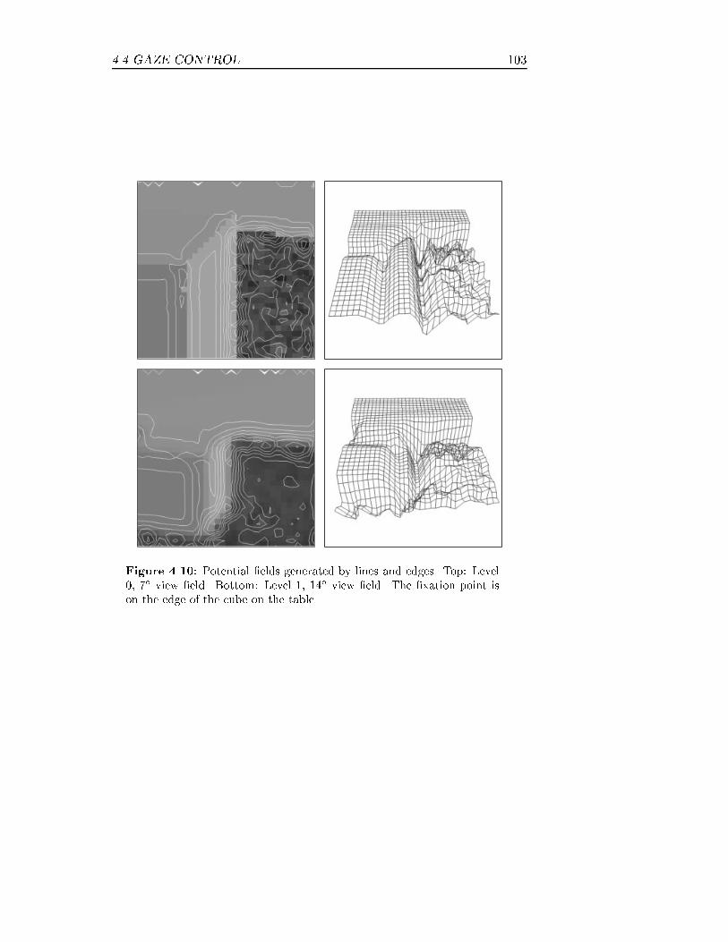
4.4 GAZE CONTROL 103
Figure 4.10: Potential �elds generated by lines and edges. Top: Level0, 7� view �eld. Bottom: Level 1, 14� view �eld. The �xation point ison the edge of the cube on the table.

104 HIERARCHICAL DATA-DRIVEN FOCUS OF ATTENTION
Figure 4.11: Potential �elds generated by lines and edges. Top: Level2,28� view �eld. Middle: Level 3, 53� view �eld. Bottom: Level 4, 90�
view �eld. The �xation point is on the edge of the cube on the table.
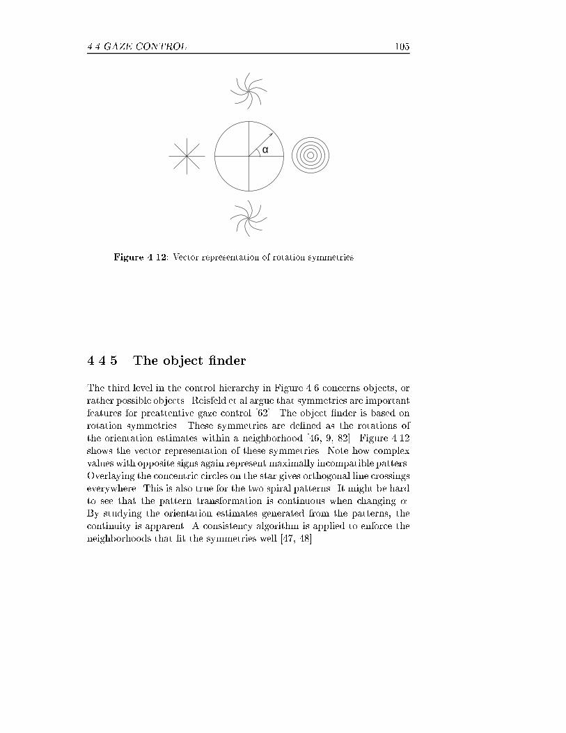
4.4 GAZE CONTROL 105
α
Figure 4.12: Vector representation of rotation symmetries.
4.4.5 The object �nder
The third level in the control hierarchy in Figure 4.6 concerns objects, orrather possible objects. Reisfeld et al argue that symmetries are importantfeatures for preattentive gaze control [62]. The object �nder is based onrotation symmetries. These symmetries are de�ned as the rotations ofthe orientation estimates within a neighborhood [46, 9, 82]. Figure 4.12shows the vector representation of these symmetries. Note how complexvalues with opposite signs again represent maximally incompatible patters.Overlaying the concentric circles on the star gives orthogonal line crossingseverywhere. This is also true for the two spiral patterns. It might be hardto see that the pattern transformation is continuous when changing �.By studying the orientation estimates generated from the patterns, thecontinuity is apparent. A consistency algorithm is applied to enforce theneighborhoods that �t the symmetries well [47, 48].

106 HIERARCHICAL DATA-DRIVEN FOCUS OF ATTENTION
Rotation symmetry estimation
The orientation estimates for the concentric circles pattern can be writtenas a function of the distance to the center and the angle to the horizontalaxis:
f(�) = f(k�k)ei2 arg(�) (4.14)
where � is the position vector from the center of the symmetry. Thecorresponding function for the star pattern is:
f(�) = f(k�k)ei2 arg(�)+� (4.15)
i.e. a phase shift of �. The spiral patterns correspond to phase shifts of��=2. The general functions is:
f(�) = f(k�k)ei�f (�) = f(k�k)ei2 arg(�)+� (4.16)
where � is determined by the pattern according to Figure 4.12.
A �lter for detecting these symmetries should display the conjugated sym-metry itself:
b(�) = b(k�k)ei�b(�) = b(k�k)e�i2 arg(�) (4.17)
where � is the position vector from the center of the �lter.
The magnitude function can be any window function. Here the magnitudeis a squared cosine function with zero magnitude in the center:
kb(�)k =
8<:cos
�r�8
�if 1 � r =
q�21 + �22 � 7
0 otherwise(4.18)
The �lter response when centered on a rotation symmetry pattern is:
s(0) =X�
f(� � �)b(�)j�=0 (4.19)
=X�
f(k0� �k)ei�f (0��)b(k�k)e�i�b(�) (4.20)
=X�
f(k�k)b(k�k)ei�f (��)��b(��) (4.21)

4.4 GAZE CONTROL 107
Use the de�nitions in Equations (4.16) and (4.17) in Equation (4.19):
s(0) =X�
f(k�k)b(k�k)ei2 arg(��)+��2 arg(��)
(4.22)
=X�
f(k�k)b(k�k)ei� (4.23)
= kskei� (4.24)
Equation (4.22) shows that the �lter, b, estimates the correct rotationsymmetry when it is centered on it. Unfortunately the �lter also respondso� center and to linear structures. The selectivity can be enhanced byusing a consistency algorithm [47, 48, 82]. This algorithm requires threeadditional �lterings with di�erent combinations of �lter and data magni-tudes. The four �lter results are:
s1 = f � b (4.25)
s2 = f � kbk (4.26)
s3 = kfk � b (4.27)
s4 = kfk � kbk (4.28)
The second convolution s2 is obtained by using the �lter magnitude as ascalar �lter on the input data. Similarly, s3 comes from using the complex�lter with the data magnitude as a scalar image. Finally, the magnitudeof the �lter is convolved with the magnitude of the data. A consistencyoperation is obtained if the four outputs are combined as:
s =s4s1 � s2s3
s4(4.29)
Figure 4.13 on the following page shows a test pattern with rotation sym-metries and the results of the symmetry detector.
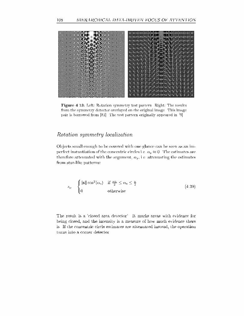
108 HIERARCHICAL DATA-DRIVEN FOCUS OF ATTENTION
Figure 4.13: Left: Rotation symmetry test pattern. Right: The resultsfrom the symmetry detector overlayed on the original image. This imagepair is borrowed from [81]. The test pattern originally appeared in [9].
Rotation symmetry localization
Objects small enough to be covered with one glance can be seen as an im-perfect instantiation of the concentric circles i.e. �s � 0. The estimates aretherefore attenuated with the argument, �s, i.e. attenuating the estimatesfrom star-like patterns:
so =
8<:ksk cos2(�s) if ��
2� �s � �
2
0 otherwise(4.30)
The result is a 'closed area detector'. It marks areas with evidence forbeing closed, and the intensity is a measure of how much evidence thereis. If the concentric circle estimates are attenuated instead, the operationturns into a corner detector.

4.4 GAZE CONTROL 109
A vector �eld pointing towards the local mass center of so is producedwith three separable �lters:
hm(�) =
8<:cos2( �1�
8) cos2( �2�
8) �7 � �1; �2 � 7
0 otherwise (4.31)
h1(�) = hm(�)�1 (4.32)
h2(�) = hm(�)�2 (4.33)
The output from hm is used both for normalization and as a rotationsymmetry certainty image:
Mm = hm � so (4.34)
The vector �eld with vectors pointing to the local mass center is:
Vm =
h1 � so=Mm
h2 � so=Mm
!(4.35)
Interpreting the vector �elds on all levels, Vjm, as gradient �elds of energy
landscapes gives the potential �elds in Figures 4.14 and 4.15. Note howa potential well is created everywhere where there is evidence for a closedcontour.

110 HIERARCHICAL DATA-DRIVEN FOCUS OF ATTENTION
Figure 4.14: Potential �elds generated by rotation symmetries. Top:Level 0, 7� view �eld. Bottom: Level 1, 14� view �eld. The �xationpoint is on the edge of the cube on the table.
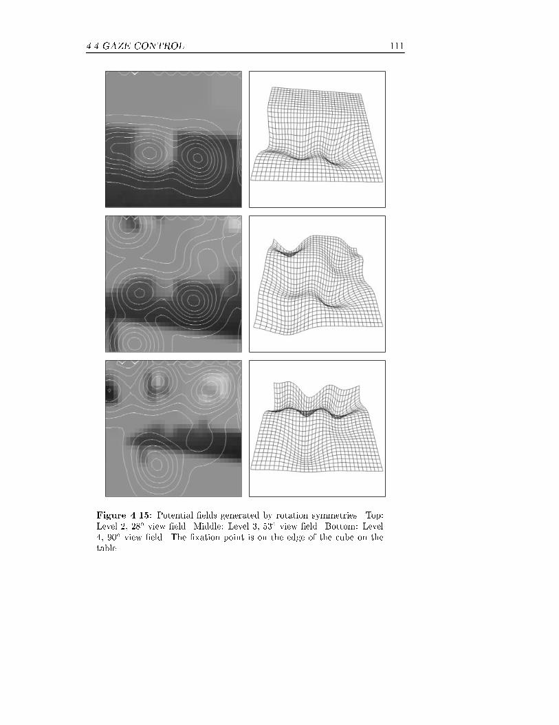
4.4 GAZE CONTROL 111
Figure 4.15: Potential �elds generated by rotation symmetries. Top:Level 2, 28� view �eld. Middle: Level 3, 53� view �eld. Bottom: Level4, 90� view �eld. The �xation point is on the edge of the cube on thetable.

112 HIERARCHICAL DATA-DRIVEN FOCUS OF ATTENTION
Pan
Tilt
0
π/2
−π/2
0 π−π
Figure 4.16: The quantization of the pan-tilt parameter space used asmemory.
4.4.6 Model acquisition and memory
So far, only processes that attract the �xation point have been considered.In Section 4.3, habituation was mentioned as a mechanism needed for anoperating focus of attention system. The basis for such a mechanism issome sort of memory.
A �rst step toward a rudimentary memory of where the system has lookedbefore is shown in Figure 4.16. It is a form of motor memory consistingof an array that quantizes the parameter space spanned by the head panand tilt angles. Since the robot moves only these two joints the parameterspace is two-dimensional and there is a one-to-one mapping to the possibleview directions.
The system remembers where it has seen something by marking the po-sitions in the memory array that corresponds to the �xation directions inwhich it has been tracking lines and edges. Bilinear interpolation is usedbetween neighboring bins. The memory is used to indicate that an edgeor a line has been tracked before and the system should move its �xationpoint elsewhere.
In a general system where many points in the parameter space mightcorrespond to looking at the same thing, an extended approach to memory

4.4 GAZE CONTROL 113
Search line
Track line
Locate object
Avoid object
N.S.
B.H.B.
O.L. L.L.
C.S.S.L.
S.L.
Figure 4.17: State transition network for the test system.
is needed. It is then important to remember not only where but also whatthe system has seen. For non-static scenes when becomes important. Thisrequires a procedure for model acquisition which is an ultimate goal forthis process.
4.4.7 System states and state transitions
The potential �elds in Figures 4.10, 4.11, 4.14 and 4.15 are weighted to-gether di�erently depending on what state the robot is currently in. Fig-ure 4.17 shows the states and the possible transitions. The transitionsbetween the states are determined by the type and quality of the data inthe �xation point. Before going into the details, an overview of the statesand the state transitions is presented.
Suppose the system is in the state of locating a possible object. It thenuses the rotation symmetry estimates on the coarser levels of the fovearepresentation. When the distance to a symmetry is small enough, (Closeto Symmetry), the system starts to search for the lines and edges of theobject. The edge tracking procedure starts when the line or edge is �xated(On Line). If the line or edge is lost, (Line Lost), the line search startsagain. The system moves away from an object when the �xation pointreturns to a position where it has tracked before, (Been Here Before).

114 HIERARCHICAL DATA-DRIVEN FOCUS OF ATTENTION
When a new symmetry is encountered, (New Symmetry), the systemstarts moving towards it. If the symmetry is lost, (Symmetry Lost),the system starts searching for linear structures that hopefully will leadtowards new interesting areas.
The camera and head parameters are calculated by de�ning an image pointto be �xated. The image point can be seen as attracting the gaze and istherefore called attracting point and is denoted v. The next �xation pointis estimated independently for the right and left cameras. The cameraorientation parameters are then calculated from an average of the two�xation points:
v =1
2(vl + vr) (4.36)
Also the system state transition is determined for the left and right viewindependently and then combined. If the transitions are not consistent,the following ranking order is used from high to low: locate object, avoidobject, track line, search line. This means that if one eye wants to switchto locate object while the other wants to continue avoiding, the systemwill switch to locate object. The reason is that one eye might catch a newobject before the other one does.
State: search line
When searching for a line or edge only the phase information is used. The�xation point should move towards and then along the valleys in Figures4.10 and 4.11. The 2D-phase information therefore has to be transformedinto vectors. This can be accomplished by a coarse to �ne approach.Figure 4.18 shows the phase �lter magnitude for a line located at � = 1 onthree scales. The �ne scale �lter has larger amplitude than the other twoclose to the line, while the coarse scale �lter has the largest amplitude at adistance. The phase values give the distance to the line as in the disparityestimation in Chapter 3. Since the magnitude is a certainty estimate, thefovea level with the highest magnitude for a given �xation point should

4.4 GAZE CONTROL 115
2 4 6 8 10 12 14 160
0.2
0.4
0.6
Pha
se fi
lter
mag
nitu
de
ξ
Figure 4.18: The phase �lter magnitude on three scales for a line locatedat � = 1.
control where to move. Let J denote the level with the largest magnitude:
kxJk = maxjkxjk (4.37)
Level J is called the controlling level. The phase angle �J gives the distanceto the line while the reference direction vector, e, de�ned in Equation ( 4.5on page 99), gives the direction to it. In order to move along an orientedstructure a vector, e?, perpendicular to e has to be chosen. There arealways two opposite alternatives when choosing e?. The alternatives areequally good, so any will do, e.g.
e? =
�e2e1
!(4.38)
The problem is now that the direction of e may ip from one point toanother, cf. regions A and F in Figure 4.8 on page 99. This makes the�xation point move back and forth over the discontinuity. Such behavioris avoided by using the direction of the last �xation point motion, vlast:
sign(vlast � e?) (4.39)
If e? changes to the opposite direction, the sign of the scalar product abovealso changes and the �xation point continues to move without changingdirection.

116 HIERARCHICAL DATA-DRIVEN FOCUS OF ATTENTION
The vector to the next �xation point, v, consists of one part directed alongthe linear structure and one perpendicular to it:
v = 2J�sign(vlast � e?)�?e? + �� �
J e�
(4.40)
The factor, 2J , compensates for the compressed distances on levels withlower resolution. The constants �? and �� control the speed of the �xationpoint motion along and towards the linear structure. �� has a naturalconnection to the �lter. Setting
�� =1
�c(4.41)
where �c is the center frequency of the �lter, makes the �xation pointmove directly to a line if it is an impulse line. Normally, the phase variesslower than this since an image mostly contains lower frequencies. Thisgives a too small value of the distance to the line which, from a controlpoint of view, is advantageous since it makes the system stable.
�? does not have such a natural interpretation as �� does. A rule of thumbis that the �xation point should not move further than the controllingfovea level can reach.
When in search line state, �� is set according to Equation (4.41), while�? is set so the motion towards the line is larger than the motion alongit:
�? = 0:25�� : (4.42)
If �? is too large and the line bends away from the tangent of the �xationpoint motion, then the �xation point might never get close to the actualline.
Figure 4.17 on page 113 shows that the only state transition from search
line is to track line (On Line). There are two conditions that have to beful�lled in order to make a transition. First, the distance to the line has tobe small enough. This can be expressed as a condition on the controllingfovea level:
J � 1 (4.43)
4.4 GAZE CONTROL 117
i.e. if one of the two �nest levels of the fovea has the maximum phasemagnitude, then the �xation point is close enough to start tracking. Sec-ond, a scale consistency condition is used in order to reduce the impact ofnoise:
keJ? � eJ+1? k � TC (4.44)
If the scalar product between the orientation estimate on the controllinglevel and the next coarser level is smaller than TC , then the estimate isconsidered to be noise and therefore discarded. Note that if, for instance,level 0 is inconsistent with level 1 but level 1 is consistent with level 2,then level 1 will be used even if level 0 has a larger magnitude. In mostexperiments, the value on the consistency threshold is:
TC =1p2
(4.45)
which is heuristically determined.
State: track line
The same information is used for tracking lines as for searching for lines.The only di�erence is that �? is now larger:
�? = ��: (4.46)
There are two possible state transitions from track line (Figure 4.17 onpage 113). The �rst one is Line Lost which returns the system to search
line if the conditions in Equations (4.43) and (4.44) no longer are ful�lled.This typically happens when a line or edge bends abruptly.
The other state transition, Been Here Before, involves the parameterspace memory array (Figure 4.16 on page 112). The memory array isupdated during the tracking. For each new �xation the correspondingmemory location is incremented with one, or rather, the four closest lo-cations are updated using bilinear interpolation. If the head returns toa position in the parameter space where it has been tracking before, and
118 HIERARCHICAL DATA-DRIVEN FOCUS OF ATTENTION
the memory value is larger than a threshold, Tm, the system changes thestate to avoid object. The value on the threshold is heuristically set to:
Tm = 3:0 (4.47)
State: avoid object
When avoiding an object, the symmetry information on the three coars-est levels is used. The intensity in the \mass image", Mm(�), (Equa-tion (4.34)) is a measure of how much evidence there is for a symmetry.The controlling level, J , is determined by searching from coarse to �ne inMm:
MJm = max
jM jm; j 2 [2; 3; 4] (4.48)
The vector, v, to the next �xation point is then:
v = �2J�sVJm (4.49)
where �s generally is set to unity.
There are two state transitions from avoid object. If the rotation symmetryinformation is lost, i.e. if
MJm = 0; (4.50)
the system returns to search line in order to �nd some structure again(Symmetry Lost).
The second state transitions concern detection of a new object (NewSymmetry). During avoid object the �xation point is moving contraryto the vector �eld Vm (Equation (4.49)). When the �xation point reachesa new symmetry, the vector VJ
m switches sign and points towards the newsymmetry, i.e. in approximately the same direction as the current motionof the �xation point. Thus, the condition for the state transition to locateobject is:
vlast �VJm > 0 (4.51)

4.4 GAZE CONTROL 119
State: locate object
When locating a new object the same information as when avoiding ob-jects is used. The only di�erence is that the �xation point now movesalong the vector �eld, Vm instead of against it. The vector to the next�xation, v, point is:
v = 2J�sVJm (4.52)
where �s generally is set to unity.
There is one state transition from locate object and that is to search line.The transition takes place if one of two conditions is ful�lled. First, as inthe avoid object case, the system starts to search for lines if the symmetryis lost (Equation (4.50)). The second condition concerns actually arrivingto a new symmetry, i.e. a potential new object. When searching for aline, a coarse to �ne approach is used. This method is not applicablefor rotation symmetries since the positions of symmetry centers are morescale-dependent. As an example, consider a square. On a coarse scalethe symmetry center is in the center of the square. On a �ne scale thereare four symmetry centers close to the corners of the square. Therefore, athreshold on the distance to the symmetry center on the controlling levelis used as a state transition condition:
kvk < Ts (4.53)
The value on Ts is half the width of the symmetry �lter:
Ts = 7 (4.54)
4.4.8 Calculating camera orientation parameters
In order to derive the orientation control parameters from the position ofan image point, a camera model has to be assumed. For physical camerasthere are a number of models ranging from a simple pinhole camera to ad-vanced simulations of light going trough aggregates of lenses. In computergraphics the pinhole camera dominates although more advanced camerasare available on some high end platforms.

120 HIERARCHICAL DATA-DRIVEN FOCUS OF ATTENTION
Kanatani [42] has derived the camera-induced motion �eld for rotationaround the camera optic center. This remains a good approximation if thedistance between the lens and true center of rotation is small comparedto the distance perpendicular to the lens to the projected objects [59].Below, the corresponding equations for how to rotate a camera in orderto �xate a certain point are derived.
The camera model
The cameras are pinhole cameras with a square sensor and with equalvertical and horizontal �elds of view. The imaging parameters are the�eld of view, , and the number of sensor elements horizontally (andvertically) across the sensor, Ne.
Neither the focal length, f , nor the physical size of the image sensor, w,are explicitly given here. The relationship between the �eld of view, theimage sensor size and the focal length is:
tan
�
2
�=
w
2f(4.55)
Resolving gives:
= 2arctan
�w
2f
�(4.56)
It is evident from Equation (4.56) that for a given �eld of view thereis an in�nite number of combinations on the focal length and the sensorwidth. The focal length often appears as a denominator, and it is thereforeconvenient to have the following convention:
f = 1:0 (4.57)
w = 2 tan
�
2
�(4.58)
we =w
Ne(4.59)
where f is the focal length, w is the \physical" sensor size, and we is thesensor element (pixel) size.

4.4 GAZE CONTROL 121
Camera pan
The optical center of the cameras coincides with the axes for the individualcamera pan joints (Figure 4.19). This makes the change in pan angle, 'cp,needed to �xate a point, P , independent of the distance between theoptical center and P :
tan('cp) =we�
f(4.60)
where � is the image coordinate. Resolving 'cp and using Equations (4.57),(4.58) and (4.59) gives the expression on the pan angle:
'cp = arctan
�2�
Netan
�
2
��(4.61)
d
x
P
w/2
f
ψ
ϕcp
ξwe
Figure 4.19: The camera seen from above. The change in the camerapan angle to �xate P , 'cp, is independent of the distance to P , since thecamera turns around the optical center.

122 HIERARCHICAL DATA-DRIVEN FOCUS OF ATTENTION
Head tilt
The head pan and tilt do not rotate the cameras around the optical center.This means that the change in head pan and tilt angles needed to �xatea point depends on the distance to the point. Although it is possible touse depth estimates, e.g. from stereo, to calculate the correct angles, itis desirable to be as independent of information from other processes aspossible. Figure 4.20 shows a side view of the head mounted on the robot
d2
d1
2x
1x
ϕ
h
ξerror
Pϕht
we
ξwe
ϕhp
Figure 4.20: The error made when the change in tilt angle 'ht is cal-culated with Equation (4.61). The image of the P will not be exactlycentered after tilting the head.
arm. If the equivalent to Equation (4.61) is used to control the head tiltangle, 'ht, the image of P is not centered. If the error is small enough, thesimplicity of using Equation (4.61) is preferable to calculating the accurateinverse kinematics. Figure 4.20 shows an example where the head is tiltedto �xate a point P . The following relations are found:
x2 = h� h cos(')d2 = L� h sin(') (4.62)

4.4 GAZE CONTROL 123
where L =qx12 + d1
2 is the initial distance from the camera center tothe P .
The new position of the image of P can be calculated from the pinholecamera equation:
we�error = fx2
d2(4.63)
Resolve �error and combine with Equations (4.62) and (4.62):
�error =f
we
h(1 � cos('))
L� h sin(')(4.64)
Finally, use Equations (4.57), (4.58) and (4.59):
�error = Ne1� cos(')
2 tan( 2)(Lh� sin('))
(4.65)
The following qualitative observations can be made regarding the size ofthe error:
1. The error decreases when the L=h ratio increases, i.e. the error issmaller for distant points.
2. The error increases when the �eld of view, , decreases, i.e. the erroris larger with a telephoto lens than with a wide angle lens.
3. The error increases with the a large change in tilt angle, i.e. a largemotion will yield a large error.
Figure 4.21 on the next page shows the error expressed as a percentage ofthe sensor width, plotted as a function of L=h for a number of tilt angles.The worst case is when the attracting point is situated on the edge of thecurrent �eld of view, i.e. when 'ht = =2.
The L=h ratio in the experiment is typically between 15 and 30 (h = 100mm and 1500 mm < L < 3000 mm), which means that the worst caseerror is about 1% corresponding to 5 pixels. This might seem as a lot,but the change in tilt angle mostly is much less the half the �eld of view.The continuous operation of the head also assures a correction in the nextiteration since the correction pan angle then is very small.

124 HIERARCHICAL DATA-DRIVEN FOCUS OF ATTENTION
5 10 15 20 25 30 350
1
2
3
4
Err
or (
%)
L / h
Figure 4.21: The �xation error expressed as percentage of the sensorwidth as a function of L=h. The �eld of view is = �=2. The error isplotted for four changes in tilt angles: ' = =2 = �=4 (dash-dotted),' = 3�=16 (dotted), ' = �=8 (dashed), ' = �=16 (solid).
Head pan
Calculating the error made for the head pan is more di�cult than forthe head tilt since it depends on the head tilt angle. In Figure 4.20 onpage 122, the head pan axis is marked out. This axis is only a true panaxis if the tilt angle is zero. When the head is maximally tilted the panaxis is parallel with the optical axes of the cameras.
When 'ht = 0 Equation (4.65) is applicable if h is set to half the camerabaseline (50 mm). The L=h ratio is then typically between 30 and 60which means that the error caused by panning is half the error caused bytilting the same angle.
The analytical head pan error equation is much more complicated thanEquation (4.65). Simulating a few representative cases gives an intuitivefeeling for the error as a function of the �eld of view, the distance, andthe tilt angle. Figure 4.22 on page 126 shows the error made when theattracting point is on the edge of the image, which is the worst case.The �eld of view is �=6 and �=2 for the left and right columns of plotsrespectively. The rows of plots show the error for a point at the distanceL = 250 mm, L = 1; 000 mm, L = 2; 500 mm, respectively. The solidcurve shows the error after one gaze shift. The dashed, dash-dotted and

4.5 EXPERIMENTAL RESULTS 125
dotted curves show the error after a second, third and fourth gaze shift.Note that the repeated gaze shifts also change the tilt angle.
The following qualitative observations can be made regarding the size oferror when changing the head pan angle:
1. The error increases when the distance increases if the tilt angle islarger than approximately �=4.
2. The error increases with the tilt angle.
Note that although the error is between 40 and 50 percent of the imagesize after the �rst gaze shift, it becomes less than 10 percent after a secondshift if the �eld of view is �=2. After three iterations the error is less than2%. The worst case is fairly rare, and for tilt angles less than �=4 theinitial error is only 15 percent of the image width.
The initial error can be minimized by using the camera pan joints incombination with the head pan. The cameras can be used for quick panchanges and when a point is �xated, the head pan can be used to ensuresymmetric vergence. This sort of control scheme is inspired by the humanvisual system and can for instance be found in [21, 60].
4.5 Experimental results
A trajectory of how the robot moves the �xation point can be found inFigure 4.23 on page 127. The middle picture on the wall shows a clearexample of how an object is �xated and then scrutinized. The systemmakes a saccade from the right picture to the center of the middle pic-ture. A state transition from locate object to track line occurs and thesystem starts tracking the periphery of the picture. When returning tothe starting point on the frame of the picture, the system saccades to thetable and continues there.

126 HIERARCHICAL DATA-DRIVEN FOCUS OF ATTENTION
0 π/8 π/4 3π/8 π/20
10
20
30
40
50
Err
or (
%)
Tilt angle (rad) 0 π/8 π/4 3π/8 π/20
10
20
30
40
50
Err
or (
%)
Tilt angle (rad)
0 π/8 π/4 3π/8 π/20
10
20
30
40
50
Err
or (
%)
Tilt angle (rad) 0 π/8 π/4 3π/8 π/20
10
20
30
40
50
Err
or (
%)
Tilt angle (rad)
0 π/8 π/4 3π/8 π/20
10
20
30
40
50
Err
or (
%)
Tilt angle (rad) 0 π/8 π/4 3π/8 π/20
10
20
30
40
50
Err
or (
%)
Tilt angle (rad)
Figure 4.22: Head pan errors as a function of tilt angle. The �eld ofview is = �=6 and = �=2 for the left and right columns of plotsrespectively. The rows of plots show the error for a point at the distanceL = 250 mm, L = 1000 mm, L = 2500 mm, respectively. The solid curveshows the error after one gaze shift. The dashed, dash-dotted and dottedcurves show the error after a second, third and fourth gaze shift.

4.5 EXPERIMENTAL RESULTS 127
Figure 4.23: A typical trajectory of the �xation point. The �xationpoint has followed the structures in the image and moved from object toobject.
In these experiments only features extracted from gray scale structureshave been used. A natural extension is to incorporate color edges [83, 79,78], texture gradients [45], etc. in order to get a better segmentation ofthe image. The potential �elds give the possibility to do this fairly easy.If for instance a color and gray scale edge coincide, the potential well willbe much deeper than if it is a gray scale edge on a region with constantcolor.
The results also show that a set of individually simple processes togethercan produce a complex and purposive behavior. When adding higherlevels to the system, they should in uence the lower ones by generatingpotential wells corresponding to interesting directions and not control thecameras directly. In this way all levels of a hierarchical system control the�xation point simultaneously.

128 HIERARCHICAL DATA-DRIVEN FOCUS OF ATTENTION

5ATTENTION CONTROL USING
NORMALIZED CONVOLUTION
5.1 Introduction
Chapter 4 describes a gaze control algorithm based on a number of simul-taneously working subsystems. In this algorithm, the gaze is attracted bya set of features in the scene, and a kind of motor memory is used to re-member earlier �xations. The three basic processes; preattentive control,attentive control and habituation are pointed out as vital for an activeobserver. The model, or memory, cannot be seen as implementing the ha-bituation function, since the �xation point has to return to the particularpoint in order to know it has already been there. The desired behavior ofthe system is to act as if certain features and events do not exist,i.e. nei-ther being attracted nor repelled by them [23]. The straightforward wayof simply \cutting out" or erasing the corresponding areas in the inputimage or the feature image does not solve the problem. The in uence ofan image structure reaches over a large area, especially at coarse resolu-tion. Erasing all points in a feature image that are in uenced by a certainimage feature removes many useful estimates as well. Erasing in the inputimage creates \objects" that generate new image features.
It can be argued that building a repelling potential �eld around known, ormodeled, structures solves the problem with the returning gaze point, butit does not. The attraction of the feature remains, but it is balanced bythe repelling potential �eld. This might cause the �xation point to stop in
129

130 ATTENTION CONTROL USING NORMALIZED CONV.
a local minimum not corresponding to any structure in the �eld of view,since it is impossible to build a �eld that exactly cancels the attracting�eld. The repelling potential �eld also forces the �xation point to movearound an already modeled structure when passing it.
Using a technique termed 'normalized convolution' when extracting theimage features allows for marking areas of the input image as unimportant.The image features from these areas are then 'invisible' and consequentlydo not attract the attention of the system, which is the desired behaviorof a habituation function.
5.2 Normalized convolution
Normalized convolution (NC) is a novel �ltering method presented byKnutsson and Westin [48]. The convolution method is designed for �l-tering of incomplete and/or uncertain data. A comprehensive theory isfound in [82]. A central concept in this theory is the separation of signaland certainty for both the �lter and the input signal.
Normalized convolution is based on viewing each �lter as a set of one ormore basis functions, bi, and a weighting window, a, called the applica-bility function. The window is used for spatial localization of the basisfunctions which may be considered to have in�nite support. Similarly, theinput signal is divided into the actual signal f and a certainty function,c. Standard convolution of a signal, s, with a set of �lters, hi can beexpressed as:
1CA =
0B@h1 � s...
hN � s
1CA =
0B@ab1 � cf
...abN � cf
1CA (5.1)
Let the normalized convolution between abi; i 2 f1; ::; Ng and cf be

5.2 NORMALIZED CONVOLUTION 131
de�ned by:
0B@f1
...fN
1CA = G�1
1CA = G�1
0B@ab1 � cf
...abN � cf
1CA (5.2)
where G is a matrix de�ned as:
G =
0B@ab1b
�1 � c : : : ab1b
�N � c
.... . .
...abNb
�1 � c : : : abNb
�N � c
1CA (5.3)
where b�i denotes the complex conjugate of bi. The matrix G is a met-ric that compensates for the non-orthogonality of the basis functions. Anumber of product �lters, abib
�j are used in order to estimate G. Note
that G depends on the certainty functions but is independent of the actualsignal. This means that if the certainty is independent of variations in thesignal over time, G�1 can be pre-calculated. Typical examples where G isconstant over time are:
� Border e�ect reduction. The signal certainty is set to one insidethe input image and to zero outside it. This reduces the e�ectscaused by the image border.
� Sparse or heterogeneous sampling. Non-Cartesian, sparse het-erogeneous sensor arrays or sensor arrays with malfunctioning sensorelements can be handled by setting the signal certainty to zero forthose points.
Filtering of an image with a number of �lters can be seen as expanding it ina set of basis functions. The �lter outputs are often used as the coordinatesof the image in that particular basis. Strictly, this is not correct since�lter outputs actually are coordinates in the dual base. Coordinates canbe transformed between the base and the dual base using the metric.Readers not familiar with dual bases can turn to [82] for an introduction.For orthonormal bases the di�erence is academic since the metric is anidentity matrix, but for non-orthonormal bases it is important. Note that

132 ATTENTION CONTROL USING NORMALIZED CONV.
an orthonormal basis can, locally, turn non-orthonormal due to variationsin the signal certainty.
The normalized convolution scheme generates the coordinates, f i, corre-sponding to the base, bi. In order to be able to compare with the �lteroutputs from ordinary �ltering the coordinates have to be transformedinto dual coordinates fi. As mentioned above this is done acting with themetric on the coordinates. Since G�1 has compensated for variations dueto the signal certainty, the metric that corresponds to full certainty shouldbe used:
G0 =
0B@ab1b
�1 � c0 : : : ab1b
�N � c0
.... . .
...abNb
�1 � c0 : : : abNb
�N � c0
1CA (5.4)
where c0 is a constant function equal to one. The dual coordinates arethen: 0
B@f01...
f0N
1CA = G0
0B@f1
...fN
1CA = G0G
�1
0B@ab1 � cf
...abN � cf
1CA (5.5)
Note that setting the input signal certainty equal to one gives G0G�1 = I
which in turn gives f0i = abi � cf = fi which corresponds to the standardconvolution in Equation (5.1).
Information about the output signal certainty is captured in the determi-nant of G. Although it is not necessary, it is convenient to have the outputcertainty in the interval [0; 1], which is accomplished by normalizing withthe determinant of G0. It is also desirable that the output certainty isequivariant with the input certainty, which means that multiplying theinput certainties with a factor � results in a multiplication of the outputcertainties by the same factor:
�cin ! �cout (5.6)
but
det(�M) = �N det(M) (5.7)

5.2 NORMALIZED CONVOLUTION 133
where N is the dimension of the matrix M . Having N basis functions,the following output certainty has been shown to work well:
cout =
�detG
detG0
� 1N
(5.8)
Converting a �ltering operation to NC
Rewriting a �ltering operation as a normalized convolution can be doneaccording to the following cookbook recipe:
1. De�ne an applicability function. The applicability function, a,has to be the same for all �lters. Often it is an ordinary windowfunction, such as a Gaussian or a squared cosine.
2. De�ne the basis functions. Or rather, de�ne the windowed basisfunctions, abi. These are the �lters from the original operation. Ifthere is no DC-�lter in the original �lter set, it has to be added (cf.Section 5.3).
3. De�ne a signal certainty function. Sometimes it is easy tode�ne a signal certainty, i.e. for laser ranging using time-of- ight,where the returning light intensity can be used. Points where nosignal is captured are then given zero certainty. If the certainty isnot given by the device generating the signal, some sort of certaintymeasure has to be constructed.
4. De�ne the signal. As in the basis function case, it is actually thesignal multiplied by the certainty, cf , that is used.
5. De�ne the scalar product functions. In order to measure thescalar product between the basis functions, a set of �lters with allpair-wise combinations of basis functions, bib
�j ; i; j 2 f1; ::; Ng, has
to be generated.
In the following section these steps are applied to performing normalizedconvolution using quadrature �lters.

134 ATTENTION CONTROL USING NORMALIZED CONV.
5.3 Quadrature �lters for normalized convolu-
tion
In earlier chapters quadrature �lters are used for orientation and localphase estimation. Some of the �lters presented in Chapter 2 are not truequadrature �lters, but the analysis below will be valid for them as well.A quadrature �lter can be seen as consisting of either complex or realbasis functions. Both ways are described below, taking the non-ring �lterin Equation (2.32) as an example.
5.3.1 Quadrature �lters for NC using real basis
functions
NC quadrature �ltering can be made using three real basis functions; aconstant function and the real and imaginary parts of the original �lter.The applicability function is a spatial localization function correspondingto a windowing function. Here it is chosen to:
kf(�)k =
8<:cos2 ��
2R if k�k < R
0 otherwise(5.9)
since this is the magnitude function of the original �lter in Equation (2.32).By this choice of applicability function we get the following basis functions:
b1(�) = 1 (5.10)
b2(�) = cos
���
R+ sin
��
R
�(5.11)
b3(�) = sin
���
R+ sin
��
R
�(5.12)
where b2 and b3 are the real and imaginary part of the �lter function.In addition to the complex basis function a constant basis function isrequired. The reason for this is that since the original �lter is insensitiveto the mean value of a signal, it is incapable of estimating the signal

5.3 QUADRATURE FILTERS FOR NORMALIZED CONV. 135
certainty level. For example, any constant certainty �eld would give zerooutput.
The basis functions can be considered to have in�nite support since theyare always multiplied by the applicability function when constructing the�lters needed:
ha(�) = ab1 = cos2��
2R(5.13)
hax(�) = ab2 = cos2��
2Rcos
���
R+ sin
��
R
�(5.14)
hay(�) = ab3 = cos2��
2Rsin
���
R+ sin
��
R
�(5.15)
hax and hay are the non-ring �lters used in the original operation. Inaddition to the �lters in Equations (5.13), (5.14) and (5.15), three product�lters have to be generated:
hax2(�) = ab1b�1 = cos2
��
2Rcos2
���
R+ sin
��
R
�(5.16)
hay2(�) = ab2b�2 = cos2
��
2Rsin2
���
R+ sin
��
R
�(5.17)
haxy(�) = ab1b�2 = cos2
��
2Rcos
���
R+ sin
��
R
�sin
���
R+ sin
��
R
�(5.18)
These three �lters are needed to measure how the correlation between thebasis functions varies with the signal certainty function. This is neces-sary in order to adjust for the signal variations induced by the certaintyfunction.
Figure 5.1 on the next page shows the �lters having radius R = 9. The�lters outputs are combined according to Equations (5.2) and (5.3):
0B@f
1
f2
f3
1CA = G�1
0B@ ha � cfhax � cfhay � cf
1CA (5.19)

136 ATTENTION CONTROL USING NORMALIZED CONV.
−8 −6 −4 −2 0 2 4 6 8
−0.2
0
0.2
0.4
ξ
ax
−8 −6 −4 −2 0 2 4 6 8
−0.2
0
0.2
0.4
ξ
ay
−8 −6 −4 −2 0 2 4 6 8
−0.2
0
0.2
0.4
ξ
a
−8 −6 −4 −2 0 2 4 6 8
−0.2
0
0.2
0.4
ξ
axx
−8 −6 −4 −2 0 2 4 6 8
−0.2
0
0.2
0.4
ξ
ayy
−8 −6 −4 −2 0 2 4 6 8
−0.2
0
0.2
0.4
ξ
axy
Figure 5.1: Non-ring NC quadrature �lters.

5.3 QUADRATURE FILTERS FOR NORMALIZED CONV. 137
with
G =
0B@ ha � c hax � c hay � chax � c hax2 � c haxy � chay � c haxy � c hay2 � c
1CA (5.20)
G is symmetric since all functions are real. If the basis functions arecomplex, G is Hermitian.
The scheme results in six �lters and nine di�erent convolutions instead oftwo �lters with one convolution each. Furthermore, a 3� 3 matrix has tobe inverted, possibly for each point.
5.3.2 Quadrature �lters for NC using complex
basis functions
In this section NC quadrature �ltering using complex basis functions in-stead of real ones is discussed. It is actually one real and one complexbasis function. Using the same applicability function as in Equation (5.13)gives the following complex basis functions:
b1(�) = 1 (5.21)
b2(�) = ei(��
R+sin
��
R ) (5.22)
The complex �lter that corresponds to ab2 can be realized as the two real�lters in Equations (5.14) and (5.15), i.e. the original even-odd �lter pair.Since one of the basis functions is constant, the correlation �lters are thesame as the original ones. The complex versions of Equations (5.19) and(5.20) are:
f1
f2
!= G�1
ha � cf
(hax + ihay) � cf
!(5.23)
and, using ab2b�2 = a,
G =
ha � c (hax � ihay) � c
(hax + ihay) � c ha � c
!(5.24)
138 ATTENTION CONTROL USING NORMALIZED CONV.
The total number of �lters is three. Counting one complex convolution astwo real makes six di�erent convolutions. The computational complexityis reduced further by the fact that the G is a 2�2 matrix, instead of 3�3,which facilitates the NC combination of �lter results.
5.3.3 Real or complex basis functions?
It is evident that using complex basis functions reduces the computationalcost signi�cantly. The real case requires nine convolutions while the thecomplex case only needs six. An important question to ask is how the twoapproaches di�er? The di�erence is best illuminated with two examples.In the �rst example, data is missing, or marked unimportant, in singlepoints. This resembles sensor element failure or some kind of point-wisedata drop-out. In the second example, regions larger than the �lters aremissing. This typically happens around the edges of an image, or whenmasking an image structure for focus of attention purposes.
The test signal is the same as in Section 2.1 and the �lters are the onesin Figure 5.1 on page 136. The performance of the two approaches ismeasured by comparing their output phase with the �lter output from anun-corrupted signal, shown in Figure 5.2 on the next page.
Let z denote the reference signal, i.e. the complex �lter response from theoriginal �lter on the un-corrupted signal, and let ~z denote the correspond-ing response from normalized convolution on the signal with partiallymissing data. The de�nition of the NC �lter response is:
~z =
8<:co (f2 + if3) if real basis functions
cof2 if complex basis functions(5.25)
where co is the output certainty given by Equation (5.8). The di�erencein phase between the reference signal and the tested signal is calculatedas:
di = z�i ~zi (5.26)
The magnitude of di contains the reference signal magnitude, the esti-mated signal magnitude and the certainty of the NC estimate. This makes

5.3 QUADRATURE FILTERS FOR NORMALIZED CONV. 139
0 20 40 60 80 100 120 1400
0.25
0.5
0.75
1
Inte
nsity
ξ
0 20 40 60 80 100 120 140 −π
−π/2
0
π/2
π
refe
renc
e ph
ase
0 20 40 60 80 100 120 1400
0.25
0.5
0.75
1
refe
renc
e m
ag.
Figure 5.2: Original input signal and quadrature �lter output.

140 ATTENTION CONTROL USING NORMALIZED CONV.
it suitable for weighting the errors, since errors in points with both highsignal amplitude and high NC certainty are more serious than others. Thefollowing four statistics are used:
m =1
n
nXi=1
arg(di) (5.27)
s2 =1
n� 1
nXi=1
(arg(di)�m)2 (5.28)
mw =
nXi=1
kdik arg(di)
nXi=1
kdik(5.29)
s2w =
nXi=1
(kdik arg(di)�mw)2
nXi=1
kdik(5.30)
Point-wise missing data
In this example, data is point-wise missing and the signal certainty is setto zero in these points. The two top rows of plots in Figure 5.3 on page 142show the signal and the certainty function. The line at � = 20 and theedge at � = 60 are missing a sample at the center of the image feature.The line at � = 100 and the edge at � = 140 have missing data in theneighborhood of, but not at, the actual feature.
The two middle rows Figure 5.3 show the quadrature �lter outputs and theerror plots. The left and right columns correspond to the real and complexbasis function respectively. The output certainty is plotted in the �fthrow. The bottom plots in both �gures show the di�erence between theestimated phase and the true phase. The error is plotted for kdk > 0:01only. The di�erence is close to zero which shows that both methods handlethe missing data well. The error statistics are listed in Table 5.1, which

5.3 QUADRATURE FILTERS FOR NORMALIZED CONV. 141
shows that the performance of the two methods is almost equivalent whenlooking at the absolute errors.
m mw s swReal basis functions -0.007 -0.009 0.275 0.030Complex basis functions -0.004 -0.016 0.196 0.054
Table 5.1: Statistics of the angular error in radians for phase estimationon point-wise missing data

142 ATTENTION CONTROL USING NORMALIZED CONV.
0 20 40 60 80 100 120 1400
0.25
0.5
0.75
1
cert
aint
yξ
0 20 40 60 80 100 120 1400
0.25
0.5
0.75
1
cert
aint
y
ξ
0 20 40 60 80 100 120 1400
0.25
0.5
0.75
1
Inte
nsity
ξ
0 20 40 60 80 100 120 1400
0.25
0.5
0.75
1
Inte
nsity
ξ
0 20 40 60 80 100 120 140 −π
−π/2
0
π/2
π
NC
Pha
se
0 20 40 60 80 100 120 140 −π
−π/2
0
π/2
π
cNC
Pha
se
0 20 40 60 80 100 120 1400
0.25
0.5
0.75
1
NC
mag
nitu
de
0 20 40 60 80 100 120 1400
0.25
0.5
0.75
1cN
C m
agni
tude
0 20 40 60 80 100 120 1400
0.25
0.5
0.75
1
NC
cer
tain
ty
0 20 40 60 80 100 120 1400
0.25
0.5
0.75
1
cNC
cer
tain
ty
0 20 40 60 80 100 120 140 −π
−π/2
0
π/2
π
NC
Pha
se e
rror
0 20 40 60 80 100 120 140 −π
−π/2
0
π/2
π
cNC
Pha
se e
rror
Figure 5.3: Results from normalized convolution using quadrature �l-ters with point-wise missing data. Compare the phase and magnitudeplots with Figure 5.2 on page 139. The bottom plots show the di�er-ence between the reference phase and the NC phase. Left: Real basisfunctions. Right: Complex basis functions.

5.3 QUADRATURE FILTERS FOR NORMALIZED CONV. 143
Large missing regions
In the test above the �lters reach over the points with missing data. Onlya few samples under the �lter are missing for each point. In the followingtest the regions of missing data are larger than the �lters. The two toprows of plots in Figure 5.4 on the next page show the signal and thecertainty function. As above, the line at � = 20 and the edge at � = 60are cut at the center, while the line at � = 100 and the edge at � = 140have missing data in the neighborhood.
When having point-wise missing data, the proper behavior of the phaseestimate is often easy to de�ne. When large regions are missing, however,it is not so easy to tell. There is no way to determine the shape of thesignal in the masked, or missing region. Take for instance the line at� = 20 and the edge at � = 60 in Figure 5.4 on the following page. Aftermasking with the input certainty they look similar. Therefore the phaseestimates also look the same. When �ltering at the edge of a certaintygap that is broader than the �lter, NC extrapolates according to the basisfunctions. In the quadrature �lter case this means that the phase cycleswith the same angular velocity as the impulse response. This behaviorgives an appropriate phase extrapolation for the line at � = 20 but givesa large error for the edge at � = 60. The output certainty is small forthese regions which explains the di�erence between the unweighted andthe weighted statistics. Again the performances of the two approaches aresimilar.
m mw s swReal basis functions 0.168 0.114 0.630 0.280Complex basis functions 0.063 0.136 0.611 0.366
Table 5.2: Error statistics for phase estimation partially missing data
Discussion on basis choice
Both the approach with real basis functions and the one with complexbasis functions yield quadrature �lter outputs that are close to the out-

144 ATTENTION CONTROL USING NORMALIZED CONV.
0 20 40 60 80 100 120 1400
0.25
0.5
0.75
1
cert
aint
yξ
0 20 40 60 80 100 120 1400
0.25
0.5
0.75
1
cert
aint
y
ξ
0 20 40 60 80 100 120 1400
0.25
0.5
0.75
1
Inte
nsity
ξ
0 20 40 60 80 100 120 1400
0.25
0.5
0.75
1
Inte
nsity
ξ
0 20 40 60 80 100 120 140 −π
−π/2
0
π/2
π
NC
Pha
se
0 20 40 60 80 100 120 140 −π
−π/2
0
π/2
π
cNC
Pha
se
0 20 40 60 80 100 120 1400
0.25
0.5
0.75
1
NC
mag
nitu
de
0 20 40 60 80 100 120 1400
0.25
0.5
0.75
1cN
C m
agni
tude
0 20 40 60 80 100 120 1400
0.25
0.5
0.75
1
NC
cer
tain
ty
0 20 40 60 80 100 120 1400
0.25
0.5
0.75
1
cNC
cer
tain
ty
0 20 40 60 80 100 120 140 −π
−π/2
0
π/2
π
NC
Pha
se e
rror
0 20 40 60 80 100 120 140 −π
−π/2
0
π/2
π
cNC
Pha
se e
rror
Figure 5.4: Results from normalized convolution using quadrature �l-ters with data missing in large regions. Compare the phase and mag-nitude plots with Figure 5.2 on page 139. The bottom plots show thedi�erence between the reference phase and the NC phase. Left: Realbasis functions. Right: Complex basis functions.

5.4 MODEL-BASED HABITUATION/INHIBITION 145
puts from the uncorrupted signal. It is important not only to estimateaccurately, but also to know when not doing so. Since weighted errors aresmallest for the approach with real basis functions, it is the best approachfrom this point of view. On the other hand, the di�erence in accuracybetween the approaches is not proportional to the di�erence in complex-ity, especially when the missing regions are smaller than the �lters. In ascale-space implementation there is likely a level of resolution where the�lters reach over the regions with missing data. The conclusion is thatcomplex basis functions give the best performance-complexity ratio forquadrature �ltering using normalized convolution.
5.4 Model-based habituation/inhibition
Normalized convolution can be used for disregarding image structures bysetting the signal certainty to zero for these structures. This ability makesNC suitable for directing the focus of attention of an active vision system.Take for instance a robot system with an arm and a camera head. Thesystem is supposed to react on objects entering the scene, or on unpre-dicted motion in the vicinity of the robot. However, it does not need toreact on known objects such as its own arm. This may seem as a simpleproblem, but in a hierarchical system, consisting of a number of moreor less independent processes, the impact of known structures is hard tosuppress. The di�erent low level processes do not, and can not, haveany knowledge about which structures are already known and which arenot. The higher levels, on the other hand, can provide information aboutthis. In the system presented here, high level processes generate certaintymasks that are set to zero certainty in areas with known structures. Thecertainty masks can be generated from estimated information of objectgeometry and/or from estimated local image features such as for exam-ple color, velocity or orientation. This means that, for instance, all blueobjects can be neglected using this technique.

146 ATTENTION CONTROL USING NORMALIZED CONV.
5.4.1 Saccade compensation
Saccades, i.e. fast camera motions made in order to �xate a new pointof interest, normally introduce strong erroneous responses after a saccadefor a period of time that depends on the �lter size in the time dimension.Note that merely shutting o� the camera during the saccade introducesstrong responses in any �ltering having temporal extent when the camerais turned back on. However, such errors can be almost completely elim-inated using normalized convolution. When the head makes a saccade,the certainty for the whole �eld of view is set to zero as long as the headmoves. The input frames are then considered to be missing data and donot in uence the motion estimation. Both the examples below containsaccade compensation.
5.4.2 Inhibition of the robot arm in uence on
low level image processing
Figure 5.5 on the next page shows a system consisting of a simulatedPuma 560 arm and a stereo camera head mounted on a neck centeredover the \waist joint". Objects are produced in the machine to the leftand a conveyor belt transports them towards a bin to the right. Figure 6.3on page 161 shows a blueprint of the scene.
Figure 5.8 on page 150 shows every 10th frame of a sequence where anobject passes the robot on the conveyor belt, while the robot arm movesback and forth along the belt. The two leftmost columns in Figure 5.8on page 150 show an overview and the right camera view. The head per-forms saccadic tracking, i.e. when the object is too far from the center ofthe image the head rapidly changes �xation point to center the object.Consequently, the head is not moving continuously. A method based onthree-dimensional quadrature �lters that can track object by smooth pur-suit is presented in [43] but is at present not implemented with normalizedconvolution.

5.4 MODEL-BASED HABITUATION/INHIBITION 147
Figure 5.5: A puma 560 robot arm by a conveyor belt. The robot hasa neck with a stereo camera head cf. the cover.
Puma CTRL
Puma arm
Head CTRL
Head
Arm modelLow level processing
Puma CTRL
Puma arm
Head CTRL
Head
Arm modelLow level processing
CamerasCameras
Certainty mask
Arm mask
Figure 5.6: Block diagram for model based inhibition of a puma robotarm.

148 ATTENTION CONTROL USING NORMALIZED CONV.
The third column of Figure 5.8 shows the pairwise temporal di�erencesbetween consecutive frames. The head tracks the local center of mass ofthe temporal di�erences. The tracking is similar to the method for locatingsymmetries described in Subsection 4.4.7. When the head is not movingand the arm is out of sight, the object appears clearly and is easy totrack. When the head makes a saccade, as in the fourth row of Figure 5.8,the whole �eld of view changes which makes tracking impossible. In thelast three rows the robot arm becomes visible and dominates the �eld ofview, which makes the head track the arm instead of the object. Boththe saccade and the robot arm are examples of known events that shouldbe inhibited from e�ecting the pre-attentive gaze control. Normalizedconvolution is applicable for both these problems.
When the head makes a saccade, the certainty for the whole �eld of viewis set to zero as long as the head moves. The input frames are thenconsidered to be missing data and do not in uence the motion estimation.In order to generate a certainty mask that cancels the motion estimatesfrom the robot arm, a model of the arm is needed. The position of thearm in relation to the camera and the joint angles for both the arm andhead are also necessary. The block diagram in Figure 5.6 on the pagebefore shows a system that takes the arm and head control parametersand generates a mask that covers the arm. The geometrical model doesnot need to be precise. A bounding box representation of each link issu�cient.
The bounding boxes are used for rendering a certainty mask directly intoa fovea representation as shown in Figure 5.7. The leftmost image showsthe �eld of view with the fovea level boundaries marked out for clarity.The other images show the certainty mask for the four levels of the fovea.The fourth column in Figure 5.8 on page 150 shows the arm mask. Thefovea is combined as described in Chapter 4. The masked area in the lowerpart of the three �rst images of the fourth column is due the boundingbox of the shoulder link.
The last column in Figure 5.8 shows the temporal di�erences using nor-malized convolution using the certainty masks in the fourth column. Onlythe object of interest is visible. The e�ects of the known events have van-

5.4 MODEL-BASED HABITUATION/INHIBITION 149
Figure 5.7: The certainty mask generated from the bounding box rep-resentation of the robot arm.
ished. In the last row, the object is behind the robot arm, and there isnaturally no way of recovering it. Note that if the bounding box repre-sentation is too crude and an object is close to the arm, the object mightbe masked out although it is visible, cf. Subsection 5.4.4. On the otherhand, if the bounding box representation is too tight and the parametersand/or arm position are imperfect, the mask might fail to cover the armcompletely.
5.4.3 Inhibition of modeled objects
The same procedure as in the last section can be applied to remove lowlevel responses from already modeled structures. Figure 5.9 on page 152shows every 10th frame of a sequence where some objects pass the roboton the conveyor belt. The two leftmost columns in this �gure show anoverview and the right camera view. The large cross-hair, in the rightcamera view, shows the current �xation point, and the small cross-hairpoints out where the head would saccade to if a saccade was to be executedimmediately. The third column shows the pairwise temporal di�erencesbetween consecutive frames.
When a new object is detected it is �xated, and a model is invoked. Thismodel contains a bounding box representation, a 3D position and a 3Dvelocity. When the model is set, a certainty mask is generated which isused for inhibiting responses from the object. The system is then sensitiveonly to un-modeled events. The masks from the object models are shownin the fourth column, while the last column contains temporal di�erencesusing normalized convolution.

150 ATTENTION CONTROL USING NORMALIZED CONV.
Figure 5.8: Inhibition of motion estimate due to known events.
5.4 MODEL-BASED HABITUATION/INHIBITION 151
In the �rst two rows the system detects a new object behind the twoalready modeled objects. When the third object is modeled, the systemmakes a saccade towards the middle object by canceling the appropriatemask. During the saccade the whole �eld of view is given zero certainty.
In the four last rows the attention is shifted between the objects by simplycanceling the mask of the object to be attended to. With this strategythe low level processes do not need to know the di�erence between anew object entering the scene and a mask being canceled, and a complexcommunication structure between high and low levels is avoided.
As long as the constant velocity model is appropriate, the projected cer-tainty mask will cover the modeled structures. However, if the model istoo simple, the corresponding certainty mask slides o�. If this happens,the previously suppressed low level responses will automatically alarm andthe system shifts the attention for updating that particular model. Whenall moving objects are modeled correctly, the lower levels of the systemwill be quiet. Only models corresponding to objects that change theirbehavior alarm and need additional attention.
5.4.4 Combining certainty masks
In Subsections 5.4.2 and 5.4.3 the certainty masks are based on geometryonly. Although this is often su�cient, it sometimes has undesired sidee�ects. The top left image in Figure 5.11 on page 154 shows a situationwhere an object is almost entirely masked by the arm although it is visible.The mask is generated according to the arm and head geometry only, anyobjects between the arm and camera are not accounted for. The middleleft image in the same �gure shows what happens if the mask instead isbased on object color only. Regions with the color of the robot arm aremasked. The color has to be extracted with methods that compensate forthe color of the illumination [56, 55]. The arm is masked correctly but the oor and the little cylindrical object to the left are masked as well. Thesolution in this case is shown in the bottom image of Figure 5.11, wherethe two previous masks are combined. The total mask should only be zerofor red objects within the bounding box representation of the arm, thus

152 ATTENTION CONTROL USING NORMALIZED CONV.
Figure 5.9: Inhibition of already modeled objects.

5.5 DISCUSSION 153
Figure 5.10: The robots view of the conveyor belt with a cylindricalobject and a box.
they are combined with a logical OR. By combinating masks from di�erentmodels or image features a more selective masking can be performed.
5.5 Discussion
It has been shown that normalized convolution can be used for attentioncontrol. By suppressing known structures, relatively simple methods canbe used in the following processing stages. Guiding attention by means ofcertainty masks �ts in a natural way in a system exploiting the bene�tsfrom separating signal from certainty [48, 82]. Since normalized convolu-tion is based on a series of convolutions, this scheme can be implementedusing special hardware for convolutions. For all levels of a feature hierar-chy the convolutions can be executed in parallel, and NC can therefore beas fast as a standard convolution.

154 ATTENTION CONTROL USING NORMALIZED CONV.
Figure 5.11: Combination of certainty masks. Top: Geometry only.Middle: Color only. Bottom: Color and geometry.

6ROBOT AND ENVIRONMENT
SIMULATOR
A robot vision simulator has been developed in the Application Visual-ization System, AVS, to facilitate testing of robot vision and control algo-rithms [86]. The simulator reduces the need for expensive special purposehardware since it can be run in \slow motion". A real-time process can beinvestigated although only limited computational resources are available.It also allows testing of di�erent types of robots and robot con�gurationswithout any extra cost. The scene can be varied from a few very simplepolyhedral objects to complex, realistic, texture mapped environments.The simulated reality, such as true 3d-structure, true distance, etc., caneasily be compared with the results obtained by the robot vision systemin order to evaluate the performance of the algorithms [20, 19].
6.1 General description of the AVS software
The AVS software is a product from Advanced Visual Systems Inc. (AVSInc.). It is an interactive visualization environment for scientists, engineersand technical professionals. AVS o�ers an environment that allows usersto construct applications incorporating their own code without graphicsprogramming. The package is easy to learn and use, it provides an intu-itive interface for quickly designing prototype applications, and it suppliespowerful tools for customization and tuning production applications.
155

156 ROBOT AND ENVIRONMENT SIMULATOR
There are two major ways of using AVS. Firstly, AVS has a number of datavisualizers called viewers. These are ready-to-use visualization packagesfor a variety of data types.
{ Image viewer is an interactive 2D image processing and display pack-age.
{ Geometry viewer is an interactive 3D geometric data renderer.
{ Graph viewer is a tool for plotting functions, measurements, statisticsusing line, bar, area, scatter and contour plots.
Secondly, AVS can be used as a prototyping tool. New algorithms andmethods can be designed and tested using visual programming, i.e. choos-ing and interconnecting program modules graphically as shown in Fig-ure 6.1 on the next page. The prototyping subsystems are:
{ Network editor, a visual programming tool.
{ Module generator, an integration tool for user-supplied code.
{ Layout editor, a graphical user interface design tool.
{ Command Language Interpreter, a scripting language and callableinterface.
AVS users can construct their own visualization applications, by combin-ing software components into executable ow networks. The components,called modules, are sub-programs or functions which are called by theAVS kernel. The ow networks are built from a menu of modules by usingdirect manipulation, a visual programming interface called the AVS Net-work Editor. With the Network Editor, the user produces an applicationby selecting a group of modules and drawing connections between them.
The AVS Command Language Interpreter (CLI) is a text language thatcan drive most of the AVS system. It can be used for making animations,

6.1 GENERAL DESCRIPTION OF THE AVS SOFTWARE 157
Figure 6.1: The AVS network editor. The window to the left is thenetwork control panel. This is the default location for module widgets.The large window is the network construction window. The upper partcontains a network editor menu to the left, and a palette of modulesin the current library to the right. The rest of the network constructionwindow is a workspace. It contains a sample network that reads an imagefrom a �le, displays it, runs a sobel operator and displays the result.
save networks, remote control, etc, Any module can pass CLI commandsto the AVS kernel, i.e. any module can modify parameters, rearrangenetworks, invoke and delete other modules, etc.
AVS includes a rich set of modules for the construction of networks. Itallows users to create their own new modules to meet their speci�c needsand dynamically load them into networks. A module generator can be usedto automatically generate module code in FORTRAN or C. Both ANSI{Cprototypes and C++ classes are available. The module generator createsskelletons for Make�les and manual pages as well.
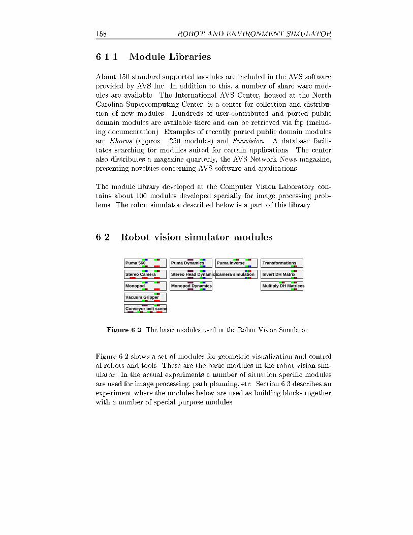
158 ROBOT AND ENVIRONMENT SIMULATOR
6.1.1 Module Libraries
About 150 standard supported modules are included in the AVS softwareprovided by AVS Inc. In addition to this, a number of share ware mod-ules are available. The International AVS Center, housed at the NorthCarolina Supercomputing Center, is a center for collection and distribu-tion of new modules. Hundreds of user-contributed and ported publicdomain modules are available there and can be retrieved via ftp (includ-ing documentation). Examples of recently ported public domain modulesare Khoros (approx. 250 modules) and Sunvision. A database facili-tates searching for modules suited for certain applications. The centeralso distributes a magazine quarterly, the AVS Network News magazine,presenting novelties concerning AVS software and applications.
The module library developed at the Computer Vision Laboratory con-tains about 100 modules developed specially for image processing prob-lems. The robot simulator described below is a part of this library.
6.2 Robot vision simulator modules
Stereo Camera
Puma 560 Puma Dynamics
Monopod Dynamics
Vacuum Gripper
Transformations
camera simulation
Puma Inverse
Invert DH Matrix
Multiply DH MatricesMonopod
Stereo Head Dynamics
Conveyor belt scene
Figure 6.2: The basic modules used in the Robot Vision Simulator.
Figure 6.2 shows a set of modules for geometric visualization and controlof robots and tools. These are the basic modules in the robot vision sim-ulator. In the actual experiments a number of situation speci�c modulesare used for image processing, path planning, etc. Section 6.3 describes anexperiment where the modules below are used as building blocks togetherwith a number of special purpose modules.

6.2 ROBOT VISION SIMULATOR MODULES 159
Puma 560
The \Puma 560" module generates a geometric description of a Puma560 robot arm with six degrees of freedom (6 DOF). The robot can bepositioned by supplying a transformation matrix to one of the input ports.The robot pose is controlled via the joint angle parameters. There arebasically three ways of furnishing joint angles. First, they can be givenmanually using the widgets on the control panel. Second, a controllingmodule can be attached to the remote control input port, passing jointangles. Finally, there is also a possibility for a module to access the jointparameter widgets using the \AVScommand" function call.
The module does not simulate the dynamics of the robot arm. In order toimplement robot dynamics and/or other forms of control parameters, a �l-ter, e.g. \Puma dynamics", can be inserted between the module supplyingthe desired joint parameter values and the \Puma 560" module.
The transformation matrix describing the location and orientation of theactuator end point is presented on an output port, enabling attachmentof di�erent tools, e.g. \vacuum gripper" or \Stereo Camera". In fact, itis possible to put one robot arm at the end of another by connecting theoutput port of one robot to the input port of another.
Stereo Camera
\Stereo Camera" creates a geometric description of a binocular camerahead with 4 DOF. The cameras have independent pans, a variable baseline,and a variable �eld of view. The camera parameters are manipulated inthe same manner as the robot arm.
The camera head is attached to an actuator by connecting the transfor-mation matrix input of \Stereo Camera" to the corresponding output of\Puma 560" or \Monopod". The transformation matrix of the actuatorend point is then transferred to the camera head, making it follow theactuator movements.
160 ROBOT AND ENVIRONMENT SIMULATOR
Note that \Stereo Camera" has three output geometry ports. One \ge-ometry viewer" module can render any number of views from the samescene, but only one can be presented on the output port. Therefore, twogeometry viewers are needed to get a stereo image pair and one extra isused for overview images. Consequently, the world representation is keptin three separate copies.
Monopod
\Monopod" is a camera head platform, or neck, with 3 DOF: pan, tilt andelevation. The hand of the robot arm and the neck have identical geome-try. The platform is positioned by furnishing a transformation matrix onone of the module input ports. If the same transformation matrix is usedfor both the robot arm and the monopod neck, the result is the con�gu-ration in Chapter 5. The neck appears to be mounted on the \shoulderlink" of the robot (see cover).
Vacuum Gripper
\Vacuum Gripper" is intended to be used together with \Conveyor belt
scene" below. It creates a geometric description of a suction cup to bepositioned at the end of a robot arm. As the name indicates, the functionis the same as lifting small objects with a vacuum cleaner hose. Themodule has a boolean parameter indicating whether the gripper is activeor not. When the suction is activated, the transformation matrix is sentto the output port.
Conveyor belt scene
\Conveyor belt scene", shown in Figure 6.3, has two conveyor belts, eachconnected to a machine. One machine produces objects, hence calledthe Producer, and puts them on a conveyor belt. The selection of type ofobject and creation time can either be externally controlled, or at random.
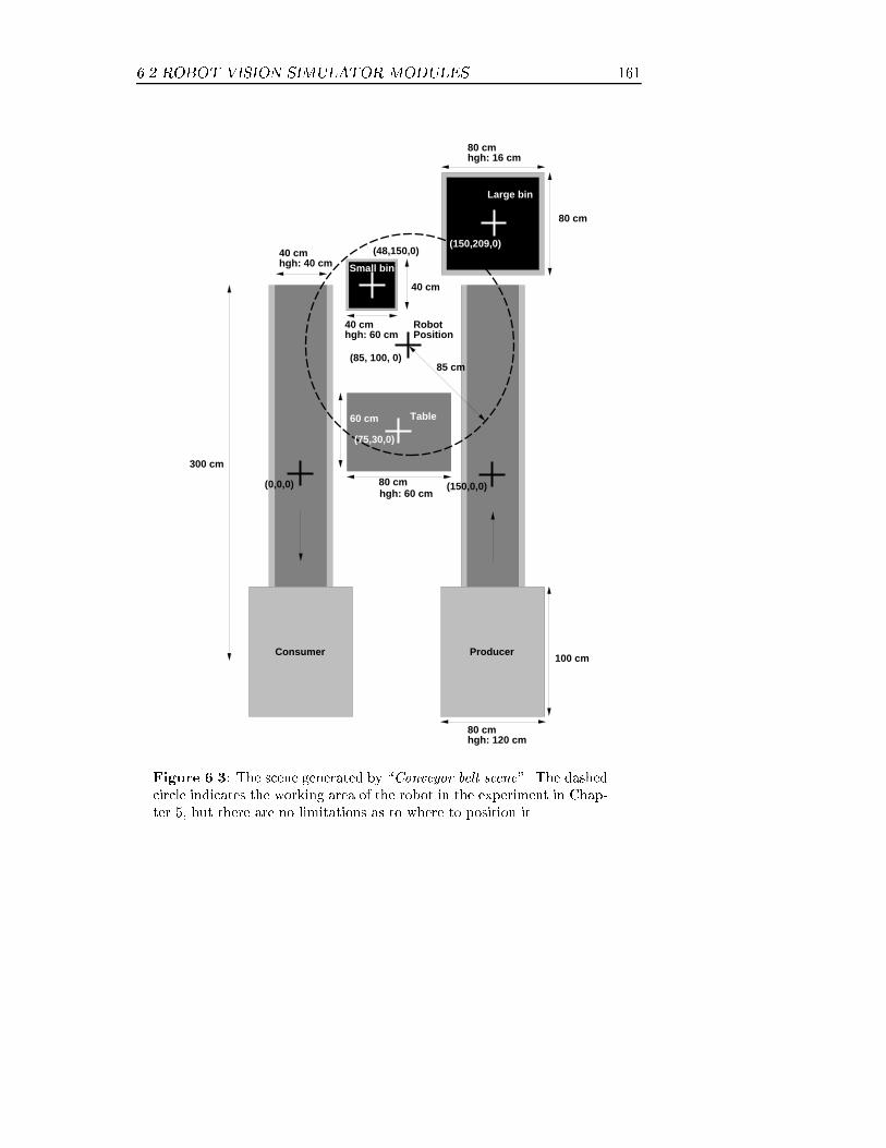
6.2 ROBOT VISION SIMULATOR MODULES 161
(0,0,0)
300 cm
80 cmhgh: 60 cm
60 cm
40 cmhgh: 40 cm
(85, 100, 0)
40 cmhgh: 60 cm
40 cm
80 cmhgh: 16 cm
80 cm
80 cmhgh: 120 cm
100 cm
(150,0,0)
(75,30,0)
(48,150,0)(150,209,0)
85 cm
RobotPosition
ProducerConsumer
Table
Large bin
Small bin
Figure 6.3: The scene generated by \Conveyor belt scene". The dashedcircle indicates the working area of the robot in the experiment in Chap-ter 5, but there are no limitations as to where to position it.
162 ROBOT AND ENVIRONMENT SIMULATOR
At the end of this belt there is a bin collecting manufactured objects.The other belt transports objects placed on it to the other machine, theConsumer, where they are consumed.
The \Vacuum Gripper" output can be attached to the module enablingmanipulation of the manufactured objects. For the robot to lift an object,it has to position the gripper close to the bounding box of the object,orient it perpendicularly to the surface, and activate the suction.
At present the simulation of physical objects and their interactions isconstrained to a few special situations. Objects are transported along theconveyor belts when put on them and fall to the oor if released in theair. The table, or the oor, can be used for temporary storage of objects.Objects can, however, be moved through each other. Piling objects is thusnot possible.
Puma Dynamics, Stereo Head Dynamics and Monopod
Dynamics
\Puma Dynamics", \Stereo Head Dynamics", \Monopod Dynamics" aremeant to implement a dynamic model of the robot arm, the camera head,and the monopod respectively. For the time being, the modules restrainthe maximum speeds with which the joints can rotate. This feature isimportant, for instance when using the robot to catch the objects in theconveyor belt scene. Not being able to move instantly from one pointin the workspace to another, the system is forced to use some kind ofpredictor.
Puma Inverse
\Puma Inverse" calculates the inverse kinematics [28], translating (if pos-sible) the desired transformation matrix of the end e�ector to robot jointangles. If both the robot transformation matrix and the end e�ector ma-trix are presented, the latter is interpreted as being in world coordinates.If only the end e�ector matrix is furnished, it is interpreted in robot cen-tered coordinates.

6.2 ROBOT VISION SIMULATOR MODULES 163
Camera simulation
Figure 6.4: Motion blur created by the \camera simulation" module.
\camera simulation" is a module for introducing noise and motion blur tothe images (Figure 6.4). The blur is controlled with a decay rate parameter0 � � � 1, where � = 1 means no blur at all and � = 0 means no imageupdate, i.e. a frozen image. The noise is controlled with a correspondingfactor 0 � � � 1 where � = 0 means no noise and � = 1 means noise only.The function for generating the output image at time t is:
iout(t) = (1� �)�� iin(t) + (1� �)iout(t��t)
�+ �N(t) (6.1)
where iout(t��t) is the preceding output image, and N(t) is a white noiseimage. The pixel values in the noise image are uniformly distributed inthe interval [0; 1[.

164 ROBOT AND ENVIRONMENT SIMULATOR
Transformations
\Transformations" produces a transformation matrix in homogeneous co-ordinates from translation, rotation, and scale parameters. The moduleis used for positioning the robot, monopod, etc.
6.3 Example of an experiment
The following example shows how a complex system can be built in AVS,see �gure 6.5. These AVS networks are used in the experiments describedin Chapter 5.
Virtual reality
Robot Vision
Object tracker dT
animated float
Occular Reflexes
Figure 6.5: This AVS network corresponds to the experiments describedin Chapter 5. The \Virtual reality" and \Robot Vision" are macro mod-ules that correspond to the networks in Figure 6.6 on page 166 andFigure 6.7 on page 168 respectively. The upstream connections to the\Virtual reality" module from \Occular re exes" are here made invisiblein order not to clutter the network.
The net is driven by \animated oat" acting as a clock pulse, activatingconnected modules. Modules not connected to the clock execute whenthey are called by upstream modules. Note that a module connected both

6.3 EXAMPLE OF AN EXPERIMENT 165
to the \animated oat" module and other upstream modules normallywait for the upstream modules to �nish before executing, but this can beoverridden by the programmer.
The \Virtual reality" module simulates the environment and generate im-ages, while the \Robot Vision" module analyses these images. These mod-ules are macro modules that contain whole networks. They are thereforeseparately described in more detail in Subsection 6.3.1.
\Object tracker dT" extracts the image point that corresponds to thecentroid of the temporal di�erences in each of the right and left images.The tracking is similar to the method for locating symmetries describedin Subsection 4.4.7. The output from the module is the vector to thecentroid in image coordinates for each image.
\Occular re exes" orients the head towards the moving object accordingto the information from the \Object tracker dT" using the tilt and panjoints on the monopod. Exactly the same control strategy as in Sub-section 4.4.8 is used since the hand of the Puma 560 is identical to theneck of the monopod. The module also verges the cameras to look at thesame point according to the disparity estimates. Note that the upstreamconnections to the \Virtual reality" module from \Occular re exes" areinvisible, but the input ports where they attach are visible. The reasonfor this is purely esthetic.
6.3.1 Macro modules
Macro modules is a way of organizing large networks into logical clustersof modules. Collecting a number of modules into a macro module doesnot e�ect the execution order of the modules. From the scheduler's pointof view all modules might as well be connected in one large network.

166 ROBOT AND ENVIRONMENT SIMULATOR
IN-> Virtual reality
OUT-> Virtual reality
Puma Inverse
Transformations
Puma 560
Vacuum Gripper
Monopod
Conveyor belt scene
geometry viewer geometry viewer
Stereo Camera
antialiasantialias
Scheduler BUG workaround
Figure 6.6: The network corresponding to the \Virtual reality" macromodule in Figure 6.5 on page 164.

6.3 EXAMPLE OF AN EXPERIMENT 167
Virtual reality
\Virtual reality" is a macro module containing the network shown i Fig-ure 6.6 on the facing page. It generates the geometric description of theconveyor belt scene, the robot arm, the camera head etc. It also ren-ders the images from the stereo camera head using the module \geometryviewer". The \antialias" modules reduce the aliasing e�ects in the im-ages by means of low pass �ltering and subsampling. The ruggedness ofedges and lines typical for computer generated images is then reduced.Note that the images has to be rendered with twice as high resolution asneeded.
\Conveyor belt scene" manages the transformation of manufactured ob-jects and handles robot interaction. Note that it is connected to the clockpulse since it calculates the dynamic behavior of the objects and thereforeneeds to know the time.
The robot hand can be positioned and oriented using any module produc-ing a transformation matrix, e.g. \Transformations". \Puma Inverse" cal-culates the inverse kinematics, translating (if possible) the desired trans-formation matrix of the end e�ector to robot joint angles.
The \Scheduler BUG workaround" module makes the network wait for allmodules in \virtual reality" before continuing. Appendix A describes whyit is necessary.
Robot Vision
Figure 6.7 shows the network corresponding to the \Robot Vision" macromodule. Log-Cartesian fovea representations of the luminance of the leftand right images are created in the \Float luminance" and \Create fovea"modules. Certainty masks are generated in \model based inhibition" bothfor the robot arm and for modeled objects as described in Chapter 5.
Phase based disparity estimates are generated by the \Robot NDCfoveastereo" module. The module uses a fovea version of the method described

168 ROBOT AND ENVIRONMENT SIMULATOR
IN-> Robot Vision
OUT-> Robot Vision
Float luminanceFloat luminance
Create fovea Create fovea
Mask signalMask signal
fovea dT fovea dT
Fovea distmass Fovea distmass
NDC oneori NDC oneori
Robot NDCfovea Stereo
model based inhinibition
Figure 6.7: The sub-network corresponding to the \Robot Vision"macro module in Figure 6.5 on page 164.

6.4 SIMULATION VERSUS REALITY 169
in Chapter 3 in combination with the normalized convolution scheme pre-sented in Chapter 5.
A vector �eld pointing towards the centroid of temporal di�erences iscreated by the \fovea dT" and \Fovea distmass". The vector �eld can beinterpreted as the gradients of a potential �eld around moving objects.
6.4 Simulation versus reality
Simulated environments are powerful tools for developing robot visionalgorithms. New robot types and con�gurations can be tested withouthaving to buy new expensive hardware. Interface, electrical and controlproblems can be bypassed. Ground truth is known. Dynamic eventscan be run in slow motion, and so forth. This blessing might, on theother hand, be a curse. Algorithms working perfectly in the simulatedenvironment might fail completely on natural images. Control strategiesmight break down due to latencies [12] in a real system that did not existin the simulated world, etc.
In order to address this problem, all feature extration algorithms have beentested on real images. The \camera simulation" module is an attempt inthis direction as well.
The control problem is harder to address. The problem of delays in theimage processing is still there in a simulated environment. The length ofthe delay is mostly constant and known, which might not correspond toa real situation. In Figure 6.5 on page 164 the network is synchronous,meaning that all modules are running according to a common clock, de�n-ing \real-time" for the entire system. This type of simulation does notre ect the di�culties of having a real-time running world and dedicatedhardware running in its own time connected to general purpose hardwareworking even slower. Another disadvantage of having a synchronous sys-tem is that it forces the higher levels to work with the same resolutionin time as the lower levels, something that probably is most ine�cient.The setup in Figure 6.8 on page 171 is a possible solution to this problem.

170 ROBOT AND ENVIRONMENT SIMULATOR
The system is spread over a number of AVS sessions, each with a separatescheduler and thus a separate clock. The sessions execute independentlyand communicate asynchronously which makes it more realistic than thesystem in Figure 6.5 on page 164. Real-time control loops are kept in\session A", while more time consuming analysis is carried out in \sessionB". There is no limit to how many AVS sessions that can be connected.Future research will explore the viability of a system such as in Figure 6.8.
6.5 Summary
The robot simulator has played a major role in the research that is thebasis for this thesis. It allows the user to gain insight in the problemsconcerning the generation of robot joint angles from visual input, withoutgetting drowned in control problems. For instance, how camera motionis enabled but also limited by the robot's degrees of freedom. Hand-eye-coordination tasks can be studied as well.
One of the demonstrators in the VAP project is built around the conveyorbelt scene in Figure 6.3 on page 161. A robot system consisting of anPuma 560 arm, a vacuum gripper, and a stereo camera head is used forinspecting manufactured machine parts. The machine parts are passingby on one conveyer belt and only correctly manufactured objects shouldbe allowed to continue to the bin. Objects with small defects are to bereturned on another conveyer belt while severely defective and any otherobject should be discarded in a special bin. If objects are arriving fasterthan the system can inspect them, a local stack, the table, can be used.
This demonstrator contains both low level reactive behaviors and highlevel planning. The research issue is to design a multi-level control pol-icy that can handle both expected and unexpected events, and adapt itsbehavior according to the situation. The experience from these experi-ments combined with the expertize on real camera heads in other membergroups enables faster progress than doing simulation only or real experi-ments only.

6.5 SUMMARY 171
AVS session A
AVS session B
Asynchronous Interface module
Environment Simulation
Real Time Image Processing:− Spat−temp filtering− Phasebased stereo− Colour transform
Real Time Control:− Vergence− Smooth pursuit− Hand−Eye coord
World TimeClock
AsynchronousCommunication
AsynchronousCommunication
Object HypothesesGeneration
Action Planner
World ModelMaintanance
Image ProcessingControl
Goal Driven FOA
Figure 6.8: A system consisting of two AVS sessions combined withasynchronous communication modules.

172 ROBOT AND ENVIRONMENT SIMULATOR

AAVS PROBLEMS AND PITFALLS
A.1 Module scheduling problems
Modules can run locally on the same host or remotely on other hosts,possibly with di�erent architectures. Modules may also run in the sameunix process saving resources and enhancing overall performance.
In Figure 6.7 on page 168 the data ow can be divided into four separatestreams which makes it possible to run groups of modules in parallel onfour di�erent hosts. In the experiments, four SUN IPX machines wereused and \Robot NDCfovea Stereo" was run on a high performance numbercruncher, Stardent GS2500.
AVS handles the scheduling of which modules to execute and when. Gen-erally it works as expected, but there are two serious bugs in the sched-uler. The �rst bug concerns the \geometry viewer" module. It is a specialmodule in the sense that it is built-in in AVS and not supplied as a sep-arate executable as most other modules. This fact seems to confuse thescheduler. Figure A.1 on the following page shows a network with a \ge-ometry viewer" in the middle. If a new geometry is read by the \readgeometry", the \geometry viewer" executes followed by \�eld math" and\display image", which is the correct behavior. Similarly, if a new imageis read by \read image" the desired behavior is that \�eld math" waitsfor \geometry viewer" to �nish before executing. Instead the \�eld math"
173

174 AVS PROBLEMS AND PITFALLS
read geomread image
geometry viewer
field math
display image
Figure A.1: A sample network that executes in an undesired order ifa new image is read with the \read image" module. The \�eld math"module will execute twice instead of waiting for the \geometry viewer"to �nish.
module executes before the \geometry viewer", and then once more whenthe \geometry viewer" has �nished. If the \geometry viewer" had beenany other module the network would have executed as expected. The\Scheduler BUG workaround" module in Figure 6.6 on page 166 solvesthe problem by stopping all data from leaving the \Virtual reality" mod-ule before all \geometry viewer" modules have executed. This solution isunsatisfactory since it requires all data to be copied from input to outputwhich is both time and memory consuming.
The second scheduler problem concerns parallel module executions andfeedback data streams. AVS can schedule parallel execution or feedbackdata streams but not both. A network containing both parallel executionand feedback data can be made to execute correctly by carefully startingup modules, but it is highly unstable. Any interaction with the networkmight cause it to start executing in an undesired order.
Both these problems might disappear with the new release of AVS (AVS6).The control structure is then completely changed giving more control tothe programmer. Time will show.

A.2 TEXTURE MAPPING PROBLEMS 175
A.2 Texture mapping problems
a b
B
A
a b
B
A
Figure A.2: Left: A texture is mapped onto an object by linear inter-polation between the image points a and b. The result is non-equidistantmapping onto the object. Right: A texture is mapped onto an object bylinear interpolation between the object coordinates A and B.
Texture mapping enhances the naturalistic look of simulated objects sincethe surface structure of real objects can be captured. It allows having de-tailed structures even though the objects are de�ned with a few polygons.
Almost all computer graphics systems, AVS included, use linear interpo-lation in image coordinates for textures. This may make a at surfacelook warped. The reason for this is shown to the left in Figure A.2, where
176 REFERENCES
the image of an object between points A and B is rendered between theimage points a and b. The dashed rays show how the texture pixels areprojected onto the object when linear interpolation in the image planeis used. The rays go through equidistant points in the image plane butare not depicted on equidistant points on the object surface. The e�ectcan be reduced by making a �ner tessellation of the surface which meansadding vertices in between A and B. The texture will then be correctlymapped in these points as well, and the distortion between the verticeswill be smaller. However, for image sequences, e.g. from moving cameras,this method is not satisfactory. Textures seem to oat around when thecamera is moved.
In principle it is possible to add the texture when creating the objects andcreate one polygon vertex for each pixel in the texture map. The objectswill then consist of patches colored according to the texture, as opposedto coloring the projected image of the objects. This method yields betterresults but is very memory and time consuming.
The appropriate method for texture mapping is shown to the right inFigure A.2. If the depth to the points is taken into account the texture ismapped onto equidistant points along the object but not onto equidistantpoints in the image plane. The reason for not using the proper approachin most computer graphics systems is that is more complex, and thus moretime consuming.

References
[1] A. L. Abbott and N. Ahuja. Surface reconstruction by dynamic in-tegration of focus, camera vergence and stereo. In Proceedings IEEE
Conf. on Computer Vision, pages 523{543, 1989.
[2] E. H. Adelson and J. R. Bergen. Spatiotemporal energy models forthe perception of motion. Jour. of the Opt. Soc. of America, 2:284{299, 1985.
[3] J. Y. Aloimonos, I. Weiss, and A. Bandopadhay. Active vision. In-ternational Journal of Computer Vision, 1(3):333{356, 1987.
[4] R. Bajcsy. Passive perception vs. active perception. In Proc. IEEE
Workshop on Computer Vision, 1986.
[5] R. Bajcsy. Active perseption. Proceedings of the IEEE, 76(8):996{1005, August 1988.
[6] D. H. Ballard. Animate vision. Technical Report 329, ComputerScience Department, University of Rochester, Feb. 1990.
[7] D. H. Ballard and A. Ozcandarli. Eye �xation and early vision: ki-netic depth. In Proceedings 2nd IEEE Int. Conf. on computer vision,pages 524{531, december 1988.
[8] S. T. Barnard and M. A. Fichsler. Computational Stereo. ACM
Comput. Surv., 14:553{572, 1982.
[9] J. Big�un. Local Symmetry Features in Image Processing. PhD thesis,Link�oping University, Sweden, 1988. Dissertation No 179, ISBN 91{7870{334{4.
[10] R. Bracewell. The Fourier Transform and its Applications. McGraw-Hill, 2nd edition, 1986.
177

178 REFERENCES
[11] C. M. Brown. The Rochester robot. Technical Report 257, ComputerScience Department, University of Rochester, Aug. 1988.
[12] C. M. Brown. Gaze control with interactions and delays. IEEE
systems, man and cybernetics, 20(1):518{527, march 1990.
[13] C. M. Brown. Prediction and cooperation in gaze control. Biologicalcybernetics, 63:61{70, 1990.
[14] K. Brunnstr�om. Active exploration of static scenes. PhD thesis, RoyalInstitute of Technology, October 1993. ISRN KTH/NA/P-93/29-SE,ISSN 1101-2250.
[15] K. Brunnstr�om, J. O. Eklundh, and T. Lindeberg. Active detectionand classi�cation of junctions by foveating with a head{eye systemguided by the scale{space primal sketch. Technical Report TRITIA-NA-P9131, CVAP, NADA, Royal Institute of Technology, Stockholm,Sweden, 1990.
[16] A. D. Calway, H. Knutsson, and R. Wilson. Multiresolution estima-tion of 2-d disparity using a frequency domain approach. In Proc.
British Machine Vision Conf., Leed, UK, September 1992.
[17] A. D. Calway, H. Knutsson, and R. Wilson. Multiresolution frequencydomain algorithm for fast image registration. In Proc. 3rd Int. Conf.
on Visual Search, Nottingham, UK, August 1992.
[18] A. Chehikian and J. L. Crowley. Fast computation of optimal semi{octave pyramids. In Proceedings of the 7th scandinavian Conf. on
image analysis, pages 18{27, Aalborg, Denmark, 1991. Pattern recog-nition of Denmark and Aalborg University.
[19] C. C. Chen and M. M. Trivedi. Savic: A simulation, visualization,and interactive control environment for mobile robots. In H.I. Chris-tensen, K.W. Bowyer, and H. Bunke, editors, Active robot vision:
camera heads, model based navigation and reactive control, volume 6of series in machine perception and arti�cal intelligence, pages 123{144. World scienti�c publishing Co. Pte. Ltd., 1993. ISBN 981-02-1321-2.
REFERENCES 179
[20] ChuXin Chen and Mohan M. Trevedi. Mobile robots with articulatedtracks and manipulators: Intelligent control and graphical interfacefor teleoperation. In Mobile Robots VII, volume 1831, pages 592{603.SPIE, 1992.
[21] H.I. Christensen, K.W. Bowyer, and H. Bunke, editors. Active robotvision: camera heads, model based navigation and reactive control,volume 6 of series in machine perception and arti�cal intelligence.World scienti�c publishing Co. Pte. Ltd., 1993. ISBN 981-02-1321-2.
[22] J. L. Crowley and H. I. Christensen, editors. Vision as Process,ESPRIT Basic Research Series. Springer-Verlag, 1994. ISBN 3-540-58143-X.
[23] S. Culhane and J. Tsotsos. An attentinal prototype for early vision.In Proccedings of the 2:nd European Conf. on computer vision, SantaMargharita Ligure, Italy, May 1992.
[24] M. M. Fleck. A topological stereo matcher. Int. Journal of ComputerVision, 6(3):197{226, August 1991.
[25] D. J. Fleet. Measurement of image velocity. Kluwer Academic Pub-lishers, 1992. ISBN 0{7923{9198{5.
[26] D. J. Fleet and A. D. Jepson. Stability of phase information. In Pro-
ceedings of IEEE Workshop on Visual Motion, pages 52{60, Prince-ton, USA, October 1991. IEEE, IEEE Society Press.
[27] D. J. Fleet, A. D. Jepson, and M. R. M. Jenkin. Phase-based disparitymeasurement. CVGIP Image Understanding, 53(2):198{210, March1991.
[28] K. S. Fu, R. C. Gonzales, and C. S. G. Lee. Robotics. McGraw HillInt. Editions, New York, 1987.
[29] D. Gabor. Theory of communication. Proc. Inst. Elec. Eng.,93(26):429{441, 1946.
[30] M. Gkstorp and C-J. Westelius. Multiresolution disparity estimation.In Proceedings of the 9th Scandinavian conference on Image Analysis,Uppsala, Sweden, June 1995. SCIA.

180 REFERENCES
[31] Mats G�okstorp. Depth Computation in Robot Vision. PhD thesis,Link�oping University. SWEDEN, S-581 83 LINK�OPING, SWEDEN,1995. Dissertation No. 377, ISBN 91-7871-522-9.
[32] G. H. Granlund. In search of a general picture processing operator.Computer Graphics and Image Processing, 8(2):155{178, 1978.
[33] G. H. Granlund. Integrated analysis-response structures for roboticssystems. Report LiTH{ISY{I{0932, Computer Vision Laboratory,Link�oping University, Sweden, 1988.
[34] G. H. Granlund and H. Knutsson. Signal Processing for Computer
Vision. Kluwer Academic Publishers, 1995. ISBN 0-7923-9530-1.
[35] G. H. Granlund, H. Knutsson, C-J Westelius, and J Wiklund. Issuesin robot vision. Image and Vision Computing, 12(3):131{148, April1994.
[36] L. Haglund. Adaptive Multidimensional Filtering. PhD thesis,Link�oping University, Sweden, S{581 83 Link�oping, Sweden, Octo-ber 1992. Dissertation No 284, ISBN 91{7870{988{1.
[37] O. Hansen and J. Bigun. Local symmetry modeling in multidimen-sional images. In Pattern Recognition Letters, Volume 13, Nr 4, 1992.
[38] D. H. Hubel. Eye, Brain and Vision, volume 22 of Scienti�c AmericanLibrary. W. H. Freeman and Company, 1988. ISBN 0{7167{5020{1.
[39] A. D. Jepson and D. J. Fleet. Scale-space singularities. InO. Faugeras, editor, Computer Vision-ECCV90, pages 50{55.Springer-Verlag, 1990.
[40] A. D. Jepson and M. Jenkin. The fast computation of disparity fromphase di�erences. In Proceedings CVPR, pages 386{398, San Diego,California, USA, 1989.
[41] B. Julesz. Early vision and focal attention. Review of Modern physics,63(3):735{772, 1991.
[42] K. Kanatani. Camera rotation invariance of image characteristics.Computer Vision, Graphics and Image Processing, 39(3):328{354,Sept. 1987.

REFERENCES 181
[43] J. Karlholm, C-J. Westelius, C-F. Westin, and H. Knutsson. Objecttracking based on the orientation tensor concept. In Proceedings of the9th Scandinavian conference on Image Analysis, Uppsala, Sweden,June 1995. SCIA.
[44] H. Knutsson. Filtering and Reconstruction in Image Processing. PhDthesis, Link�oping University, Sweden, 1982. Diss. No. 88.
[45] H. Knutsson and G. H. Granlund. Fourier domain design of line andedge detectors. In Proceedings of the 5th International Conference on
Pattern Recognition, Miami, Florida, December 1980.
[46] H. Knutsson, G. H. Granlund, and J. Bigun. Apparatus for detectingsudden changes of a feature in a region of an image that is dividedinto descrete picture elements. Swedish patent 8502571-6 (US-Patent4.747.150, 1988, 1986.
[47] H. Knutsson, M. Hedlund, and G. H. Granlund. Apparatus for de-termining the degree of consistency of a feature in a region of animage that is divided into descrete picture elements. Swedish patent8502570-8 (US-Patent 4.747.152, 1988), 1986.
[48] H. Knutsson and C-F Westin. Normalized and di�erential convolu-tion: Methods for interpolation and �ltering of incomplete and un-certain data. In Proceedings of IEEE Computer Society Conference
on Computer Vision and Pattern Recognition, New York City, USA,June 1993. IEEE.
[49] H. Knutsson, C-F Westin, and C-J Westelius. Filtering of uncer-tain irregularity sampled multidimensional data. In Twenty-seventh
Asilomar Conf. on Signals, Systems & Computers, Paci�c Grove,California, USA, November 1993. IEEE.
[50] E. Krotkov. Exploratory visual sensing for determining spatial lay-
out with an agile stereo camera system. PhD thesis, University ofPennsylvenia, April 1987.
[51] K. Langley, T. J. Atherton, R. G. Wilson, and M. H. E. Larcombe.Vertical and horizontal disparities from phase. In O. Faugeras, editor,Computer Vision-ECCV90, pages 315{325. Springer-Verlag, April1990.

182 REFERENCES
[52] J. C. Latombe. Robot Motion Planning. Kluwer Academic Publishers,1991. ISBN 0-7923-9129-2.
[53] B. Maclennan. Gabor representations of spatiotemporal visual im-ages. Technical Report CS-91-144, Computer Science Department,University of Tennesse, September 1981.
[54] D. Marr. Vision. W. H. Freeman and Company, New York, 1982.
[55] J. Matas, R. Marik, and J. Kittler. Generation, veri�cation andlocalisation of object hypotheses based on colour. In British Machine
Vision Conference, pages 539{548, 1993.
[56] J. Matas, R. Marik, and J. Kittler. Illumination invariant colourrecognition. In E. Hancock, editor, British Machine Vision Confer-
ence, pages 469{479. BMVA, BMVA Press, 1994.
[57] R. Milanese. Focus of attention in human vision: a survey. Techni-cal Report 90.03, Computing Science Center, University of Geneva,Geneva, August 1990.
[58] R. Milanese. Detection of salient features for focus of attention. InProc. of the 3rd Meeting of the Swiss Group for Arti�cial Intelligence
and Cognitive Science, Biel-Bienne, October 1991. World Scienti�cPublishing.
[59] D. Murray and A. Basu. Motion tracking with an active camera.IEEE Transactions on Pattern Analysis and Machine Intelligence,16(5):449{459, May 1994.
[60] K. Pahlavan. Active robot vision and primary occular re exes. PhDthesis, Royal Institute of Technology, May 1993. ISSN 1101-2250.
[61] L. H. Quam. Hierarchicl warp stereo. In Proceedings from DARPA
Image understanding workshop, pages 149{155, 1984.
[62] D. Reisfeld, H. Wolfson, and Y. Yeshurun. Context free attentionaloperators: the generalized symmetry transform. International Jour-nal of Computer Vision, 1994. special issue on qualitative vision.
[63] T. D. Sanger. Stereo disparity computation using gabor �lters. Bio-logical cybernetics, 59:405{418, 1988.
REFERENCES 183
[64] E. L. Schwartz. Computational anatomy and functional architecturof striate cortex: A spatial mapping approach to perceptual coding.Vision Reasearch, 20:645{669, 1980.
[65] M. Tistarelli and G. Sandini. Direct estimation of time{to{impactfrom optical ow. In Proceedings of IEEE Workshop on Visual Mo-
tion, pages 52{60, Princeton, USA, October 1991. IEEE, IEEE Soci-ety Press.
[66] J. K. Tsotsos. Localizing stimuli in a sensory �eld using an inhibitoryattentinal beam. Technical Report RBCV{TR{91{37, Department ofComputer Science, University of Toronto, October 1991.
[67] J. K. Tsotsos. On the relative complexity of active vs. passive visualsearch. Int. Journal of Computer Vision, 7(2):127{142, Januari 1992.
[68] J. van der Spiegel, G. Kreider, C. Claeys, I. Debusschere, G. Sandini,P. Dario, F. Fantini, P. Bellutti, and G. Soncini. A foveated retina-like sensor using ccd technology. In C. Mead and M. Ismael, editors,Analog VLSI implementation of neural systems. Kluwer, 1989.
[69] Esprit basic research action 3038, vision as process, �nal report.Project document, April 1992.
[70] J. Y. A. Wang and E. H. Adelson. Layered representation for mo-tion analysis. In IEEE Conference on Computer Vision and Pattern
Recognition, pages 361{366, June 1993.
[71] J. Weng. Image matching using the windowed Fourier phase. Inter-national Journal of Computer Vision, 11(3):211{236, March 1993.
[72] C-J Westelius. Preattentive gaze control for robot vision, June 1992.Thesis No. 322, ISBN 91{7870{961{X.
[73] C-J. Westelius and H. Knutsson. Hierarchical disparity estimation us-ing quadrature �lter phase. International journal on computer vision,1995. Special issue on stereo, (submitted).
[74] C-J Westelius, H. Knutsson, and G. H. Granlund. Focus of atten-tion control. Report LiTH{ISY{I{1140, Computer Vision Laboratory,Link�oping University, Sweden, 1990.

184 REFERENCES
[75] C-J Westelius, H. Knutsson, and G. H. Granlund. Focus of attentioncontrol. In Proceedings of the 7th Scandinavian Conference on Image
Analysis, pages 667{674, Aalborg, Denmark, August 1991. PatternRecognition Society of Denmark.
[76] C-J Westelius, H. Knutsson, and G. H. Granlund. Preattentive gazecontrol for robot vision. In Proceedings of Third International Con-
ference on Visual Search. Taylor and Francis, 1992.
[77] C-J Westelius, H. Knutsson, and J. Wiklund. Robust vergence con-trol using scale{space phase information. Report LiTH-ISY-I-1363,Computer Vision Laboratory, Link�oping University, Sweden, 1992.
[78] C-J Westelius and C-F Westin. A colour representation for scale-spaces. In The 6th Scandinavian Conference on Image Analysis, pages890{893, Oulu, Finland, June 1989.
[79] C-J Westelius and C-F Westin. Representation of colour in image pro-cessing. In Proceedings of the SSAB Conference on Image Analysis,Gothenburg, Sweden, March 1989. SSAB.
[80] C-J. Westelius, C-F. Westin, and H. Knutsson. Focus of attentionmechanisms using normalized convolution. IEEE Trans on Robotics
and Automation, 1996. Special section on robot vision. (submitted).
[81] C-F Westin. Feature extraction based on a tensor image description,September 1991. Thesis No. 288, ISBN 91{7870{815{X.
[82] C-F Westin. A Tensor Framework for Multidimensional Signal
Processing. PhD thesis, Link�oping University, Sweden, S{581 83Link�oping, Sweden, 1994. Dissertation No 348, ISBN 91{7871{421{4.
[83] C-F Westin and C-J Westelius. A colour model for hierarchical imageprocessing. Master's thesis, Link�oping University, Sweden, Augustv1988. LiTH{ISY{EX{0857.
[84] J. Wiklund and H. Knutsson. A generalized convolver. In Proceed-
ings of the 9th Scandinavian conference on Image Analysis, Uppsala,Sweden, June 1995. SCIA.

REFERENCES 185
[85] J. Wiklund, C-J Westelius, and H. Knutsson. Hierarchical phasebased disparity estimation. In Proceedings of 2nd Singapore Inter-
national Conference on Image Processing. IEEE Singapore Section,September 1992.
[86] J. Wiklund, C-F Westin, and C-J Westelius. AVS, Application Vi-sualization System, software evaluation report. Report LiTH-ISY-R-1469, Computer Vision Laboratory, S{581 83 Link�oping, Sweden,1993.
[87] R. Wilson and H. Knutsson. A multiresolution stereopsis algorithmbased on the Gabor representation. In 3rd International Conference
on Image Processing and Its Applications, pages 19{22, Warwick,Great Britain, July 1989. IEE. ISBN 0 85296382 3 ISSN 0537{9989.
[88] A. L. Yarbus. Eye movements and vision. Plenum, New York, 1969.

186 REFERENCES