fnce 926 empirical methods in cffnce 926 empirical methods in cf professor todd gormley lecture 11...

FNCE 926 Empirical Methods in CF

Professor Todd Gormley

Lecture 11 – Standard Errors & Misc.

Announcements

n  Exercise #4 is due n  Final exam will be in-class on April 26

q  After today, only two more classes of new material, structural & experiments

q  Practice exam available on Canvas

2

Background readings for today

n  Readings for standard errors q  Angrist-Pischke, Chapter 8 q  Bertrand, Duflo, Mullainathan (QJE 2004) q  Petersen (RFS 2009)

n  Readings for limited dependent variables q  Angrist-Pischke, Sections 3.4.2 and 4.6.3 q  Greene, Section 17.3

3

n  Quick review of last lecture on matching n  Discuss standard errors and clustering

q  “Robust” or “Classical”? q  Clustering: when to do it and how

n  Discuss limited dependent variables n  Student presentations of “Matching” papers

Outline for Today

4

Quick Review [Part 1]

n  Matching is intuitive method

q  For each treated observation, find comparable untreated observations with similar covariates, X

n  They will act as estimate of unobserved counterfactual n  Do the same thing for each untreated observation

q  Take average difference in outcome, y, of interest across all X to estimate ATE

5


n  But, what are necessary assumptions for this approach to estimate ATE?

q  Answer #1 = Overlap… Need both treated and control observations for X’s

q  Answer #2 = Unconfoundedness… Treatment is as good as random after controlling for X

6


n  Matching is just a control strategy!

q  It does NOT control for unobserved variables that might pose identification problems

q  It is NOT useful in dealing with other problems like simultaneity and measurement error biases

n  Typically used as robustness check on OLS or way to screen data before doing OLS

7


n  Relative to OLS estimate of treatment effect…

q  Matching basically just weights differently q  And, doesn’t make functional form assumption

n  Angrist-Pischke argue you typically won’t find large difference between two estimates if you have right X’s and flexible controls for them in OLS

8


n  Many choices to make when matching

q  Match on covariates or propensity score? q  What distance metric to use? q  What # of observations?

n  Will want to show robustness of estimate to various different approaches

9

n  Getting your standard errors correct

q  “Classical” versus “Robust” SE q  Clustered SE

n  Limited dependent variables

Standard Errors & LDVs – Outline

10

n  It is important to make sure we get our standard errors correct so as to avoid misleading or incorrect inferences

q  E.g. standard errors that are too small will cause us to reject the null hypothesis that our estimated β’s are equal to zero too often

n  I.e. we might erroneously claim to found a “statistically significant” effect when none exists

Getting our standard errors correct

11

n  One question that typically comes up when trying figure out the appropriate SE is homoskedasticity versus heteroskedasiticity

q  Homoskedasticity assumes the variance of the residuals, u, around the CEF, does not depend on the covariates, X

q  Heteroskedasticity doesn’t assume this

Homoskedastic or Heteroskedastic?

12

n  What do the default standard errors reported by programs like Stata assume?

q  Answer = Homoskedasticity! This is what we refer to as “classical” standard errors

n  As we discussed in earlier lecture, this is typically not a reasonable assumption to make

n  “Robust” standard errors allow for heteroskedasticity and don’t make this assumption

“Classical” versus “Robust” SEs [Part 1]

13

n  Putting aside possible “clustering” (which we’ll discuss shortly), should you always use robust standard errors?

q  Answer = Not necessarily! Why?

n  Asymptotically, “classical” and “robust” SE are correct, but both suffer from finite sample bias, that will tend to make them too small in small samples

n  “Robust” can sometimes be smaller than “classical” SE because of this bias or simple noise!

“Classical” versus “Robust” SEs [Part 2]

14

n  Finite sample bias is easily corrected in “classical” standard errors [Note: this is done automatically by Stata]

n  This is not so easy with “robust” SEs…

q  Small sample bias can be worse with “robust” standard errors, and while finite sample corrections help, they typically don’t fully remove the bias in small samples

Finite sample bias in standard errors

15

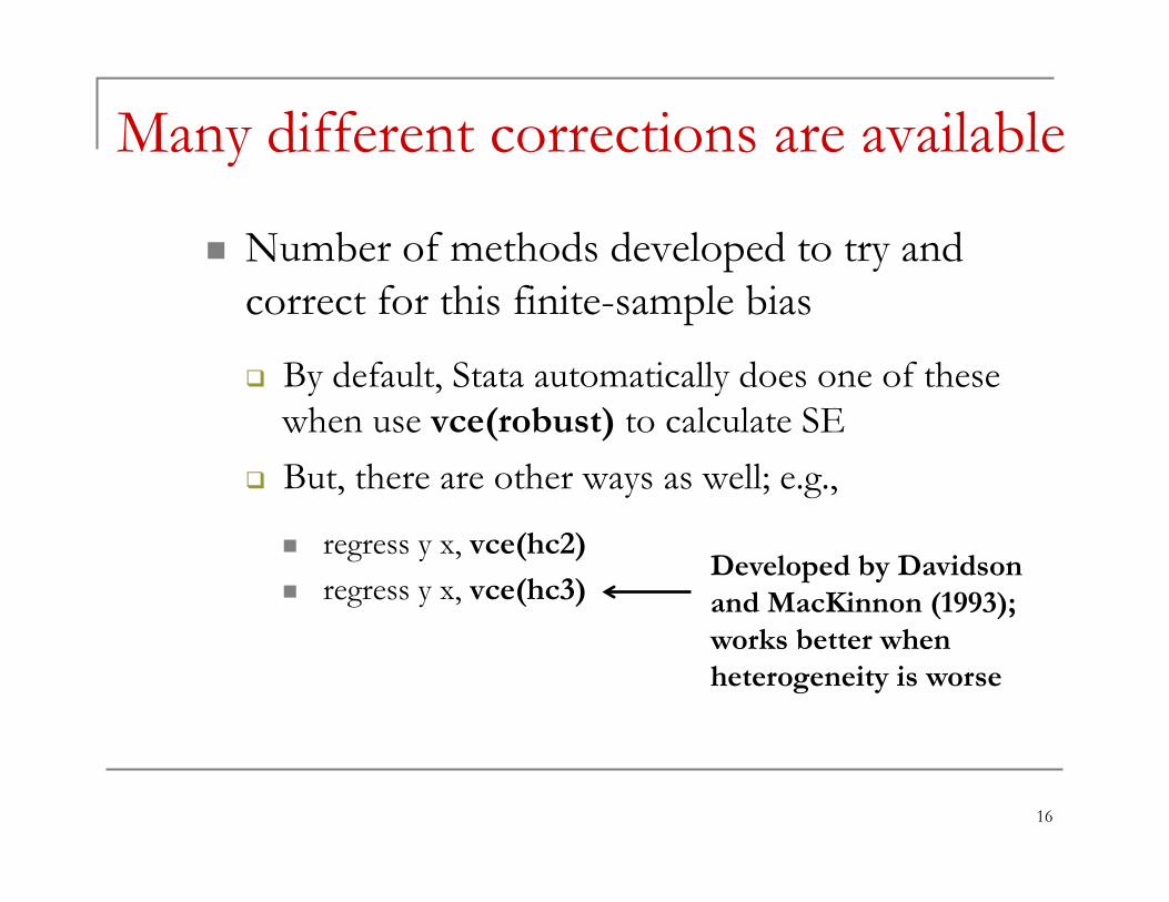
n  Number of methods developed to try and correct for this finite-sample bias

q  By default, Stata automatically does one of these when use vce(robust) to calculate SE

q  But, there are other ways as well; e.g.,

n  regress y x, vce(hc2) n  regress y x, vce(hc3)

Many different corrections are available

16

Developed by Davidson and MacKinnon (1993); works better when heterogeneity is worse

n  Compare the robust SE to the classical SE and take maximum of the two

q  Angrist-Pischke argue that this will tend to be closer to the true SE in small samples that exhibit heteroskedasticity

n  If small sample bias is real concern, might want to use HC2 or HC3 instead of typical “robust” option

n  While SE using this approach might be too large if data is actually homoskedastic, this is less of concern

Classical vs. Robust – Practical Advice

17



n  Violation of independence and implications n  How big of a problem is it? And, when? n  How do we correct for it with clustered SE? n  When might clustering not be appropriate?



18

n  “Classical” and “robust” SE depend on assumption of independence

q  i.e. our observations of y are random draws from some population and are hence uncorrelated with other draws

q  Can you give some examples where this is likely an unrealistic in CF? [E.g. think of firm-level capital structure panel regression]

Clustered SE – Motivation [Part 1]

19

n  Example Answers

q  Firm’s outcome (e.g. leverage) is likely correlated with other firms in same industry

q  Firm’s outcome in year t is likely correlated to outcome in year t-1, t-2, etc.

n  In practice, independence assumption is often unrealistic in corporate finance


20

n  Moreover, this non-independence can cause significant downward biases in our estimated standard errors

q  E.g. standard errors can easily double, triple, etc. once we correct for this!

q  This is different than correcting for heterogeneity (i.e. “Classical” vs. “robust”) tends to increase SE, at most, by about 30% according to Angrist-Pischke


21

n  Violations tend to come in two forms

#1 – Cross-sectional “Clustering”

n  E.g. outcome, y, [e.g. ROA] for a firm tends to be correlated with y of other firms in same industry because they are subject to same demand shocks

#2 – “Time series correlation”

n  E.g. outcome, y, [e.g. Ln(assets)]for firm in year t tends to be correlated with the firm’s y in other years because there serial correlation over time

Example violations of independence

22

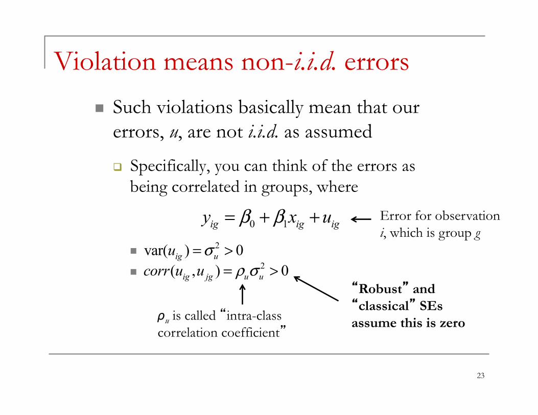
n  Such violations basically mean that our errors, u, are not i.i.d. as assumed

q  Specifically, you can think of the errors as being correlated in groups, where

n  n 

Violation means non-i.i.d. errors

23

0 1ig ig igy x uβ β= + +2var( ) 0ig uu σ= >

2( , ) 0ig jg u ucorr u u ρ σ= >“Robust” and “classical” SEs assume this is zero ρu is called “intra-class

correlation coefficient”

Error for observation i, which is group g

n  Key idea: errors are correlated within groups (i.e. clusters), but not correlated across them

q  In cross-sectional setting with one time period, cluster might be industry; i.e. obs. within industry correlated but obs. in different industries are not

q  In time series correlation, you can think of the “cluster” as the multiple observations for each cross-section [e.g. obs. on firm over time are the cluster]

“Cluster” terminology

24

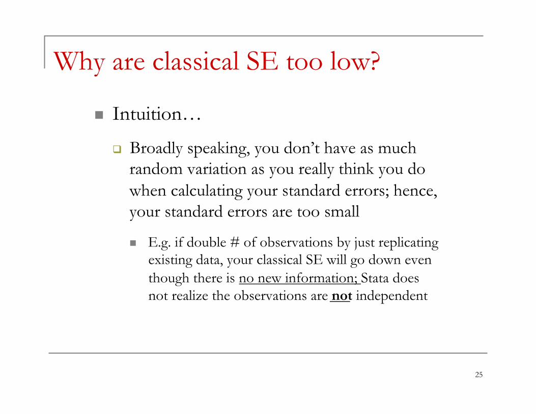
n  Intuition…

q  Broadly speaking, you don’t have as much random variation as you really think you do when calculating your standard errors; hence, your standard errors are too small

n  E.g. if double # of observations by just replicating existing data, your classical SE will go down even though there is no new information; Stata does not realize the observations are not independent

Why are classical SE too low?

25






26

n  By assuming a structure for the non-i.i.d. nature of the errors, we can derive a formula for are large the bias will be

n  Can also see that two factors are key

q  Magnitude of intra-class correlation in u q  Magnitude of intra-class correlation in x

How large, and what’s important?

27

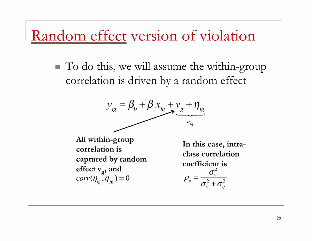
n  To do this, we will assume the within-group correlation is driven by a random effect

All within-group correlation is captured by random effect vg, and

Random effect version of violation

28

yig = β0 + β1xig + vg +ηig

uig

!"#

( , ) 0ig jgcorr η η =2

2 2v

uv η

σρσ σ

=+

In this case, intra-class correlation coefficient is

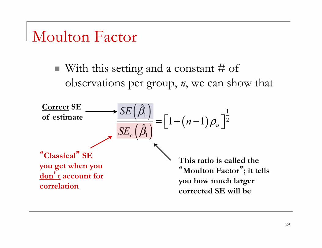
n  With this setting and a constant # of observations per group, n, we can show that

Moulton Factor

29

( )( ) ( )

112

1

ˆ1 1

ˆ uc

SEn

SE

βρ

β⎡ ⎤= + −⎣ ⎦

Correct SE of estimate

“Classical” SE you get when you don’t account for correlation

This ratio is called the “Moulton Factor”; it tells you how much larger corrected SE will be

q  Interpretation = If corrected for this non-i.i.d. structure within groups (i.e. clustering) classical SE will larger by factor equal to Moultan Factor

n  E.g. Moultan Factor = 3 implies your standard errors will triple in size once correctly account for correlation!

Moulton Factor – Interpretation

30

( )( ) ( )

112

1

ˆ1 1

ˆ uc

SEn

SE

βρ

β⎡ ⎤= + −⎣ ⎦

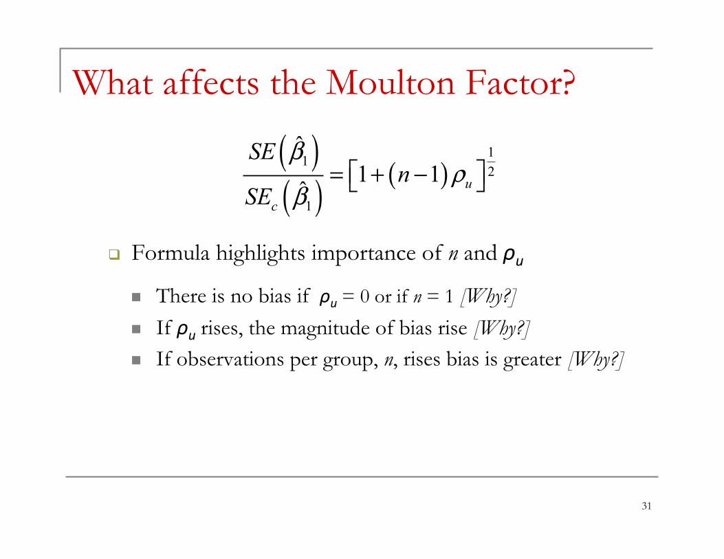
q  Formula highlights importance of n and ρu

n  There is no bias if ρu = 0 or if n = 1 [Why?] n  If ρu rises, the magnitude of bias rise [Why?] n  If observations per group, n, rises bias is greater [Why?]

What affects the Moulton Factor?

31

( )( ) ( )

112

1

ˆ1 1

ˆ uc

SEn

SE

βρ

β⎡ ⎤= + −⎣ ⎦

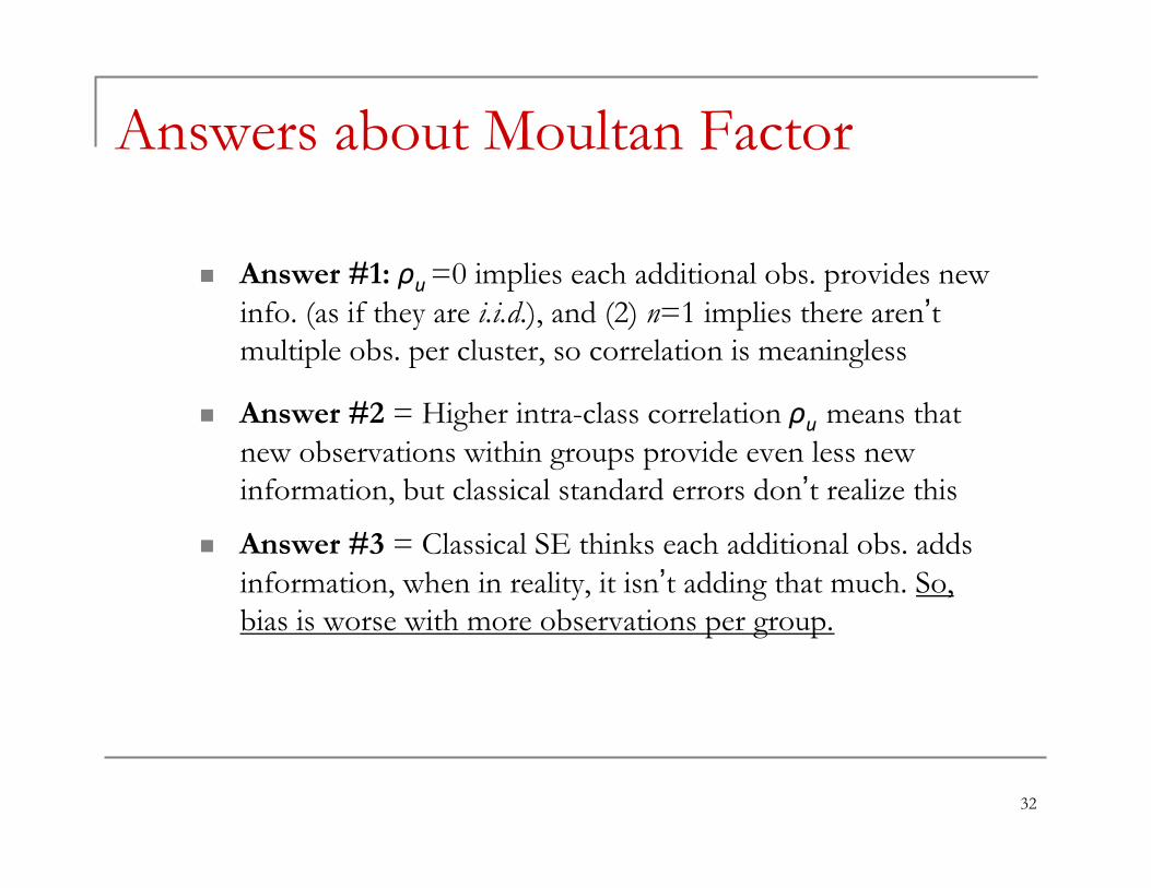
n  Answer #1: ρu =0 implies each additional obs. provides new info. (as if they are i.i.d.), and (2) n=1 implies there aren’t multiple obs. per cluster, so correlation is meaningless

n  Answer #2 = Higher intra-class correlation ρu means that new observations within groups provide even less new information, but classical standard errors don’t realize this

n  Answer #3 = Classical SE thinks each additional obs. adds information, when in reality, it isn’t adding that much. So, bias is worse with more observations per group.

Answers about Moultan Factor

32

n  Moultan Factor basically shows that downward bias is greatest when…

q  Dependent variable is highly correlated across observations within group [e.g. high time series correlation in panel]

q  And, we have a large # of observations per group [e.g. large # of years in panel data]

Bottom line…

33

Expanding to uneven group sizes, we see that one other factor will be important as well…

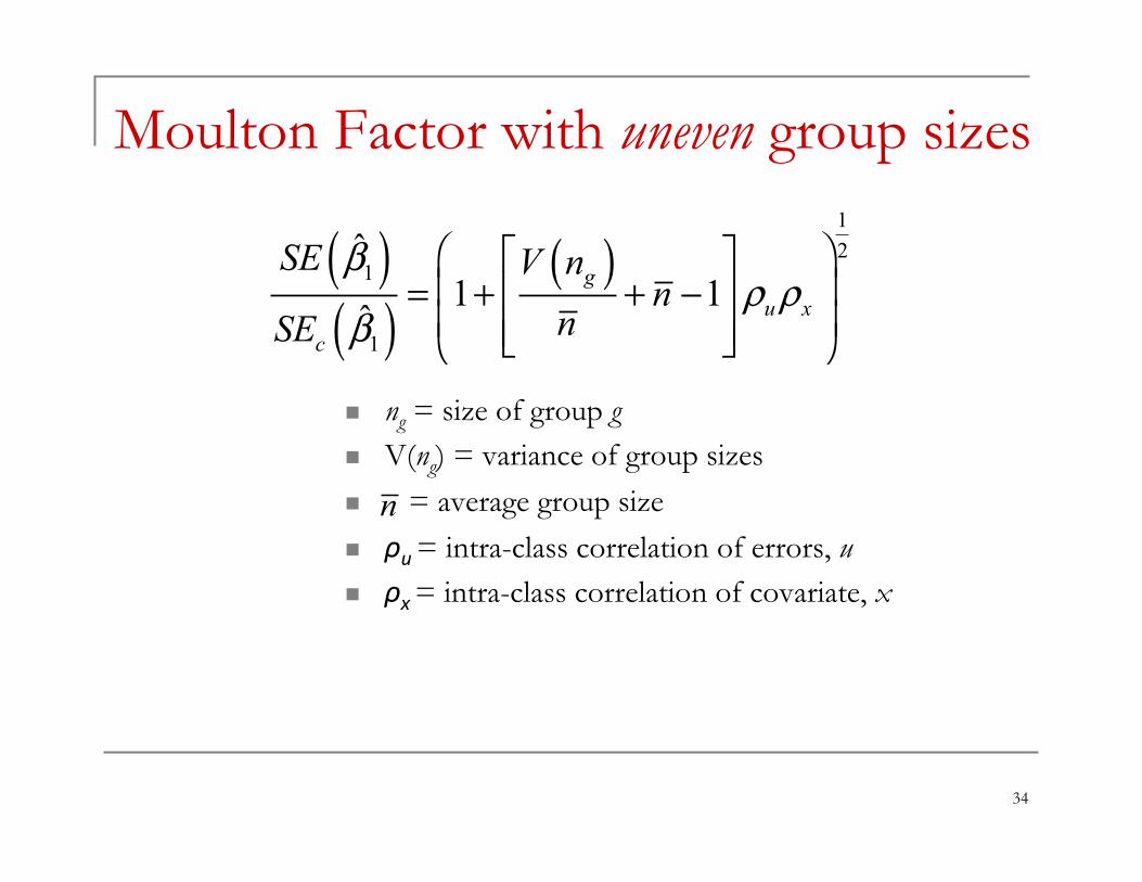
n  ng = size of group g n  V(ng) = variance of group sizes

n  = average group size n  ρu = intra-class correlation of errors, u n  ρx = intra-class correlation of covariate, x

Moulton Factor with uneven group sizes

34

( )( )

( )12

1

1

ˆ1 1

ˆg

u xc

SE V nn

nSE

βρ ρ

β

⎛ ⎞⎡ ⎤⎜ ⎟= + + −⎢ ⎥⎜ ⎟⎢ ⎥⎣ ⎦⎝ ⎠

n

Importance of non-i.i.d. x’s [Part 1]

35

( )( )

( )12

1

1

ˆ1 1

ˆg

u xc

SE V nn

nSE

βρ ρ

β

⎛ ⎞⎡ ⎤⎜ ⎟= + + −⎢ ⎥⎜ ⎟⎢ ⎥⎣ ⎦⎝ ⎠

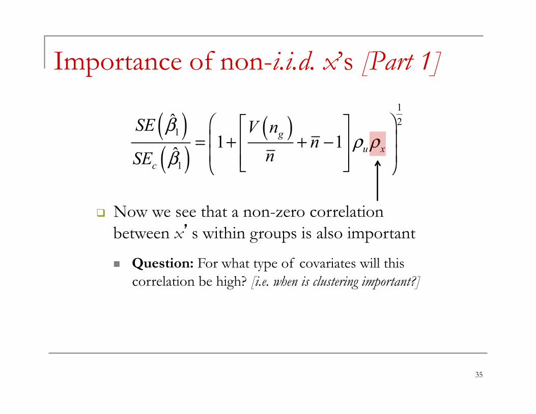
q  Now we see that a non-zero correlation between x’s within groups is also important

n  Question: For what type of covariates will this correlation be high? [i.e. when is clustering important?]

n  Prior formula shows that downward bias will also be bigger when…

q  Covariate only varies at group level; px will be exactly equal to 1 in those cases!

q  When covariate likely has a lot of time series dependence [e.g. Ln(assets) of firm]

Importance of non-i.i.d. x’s [Part 2]

36






37

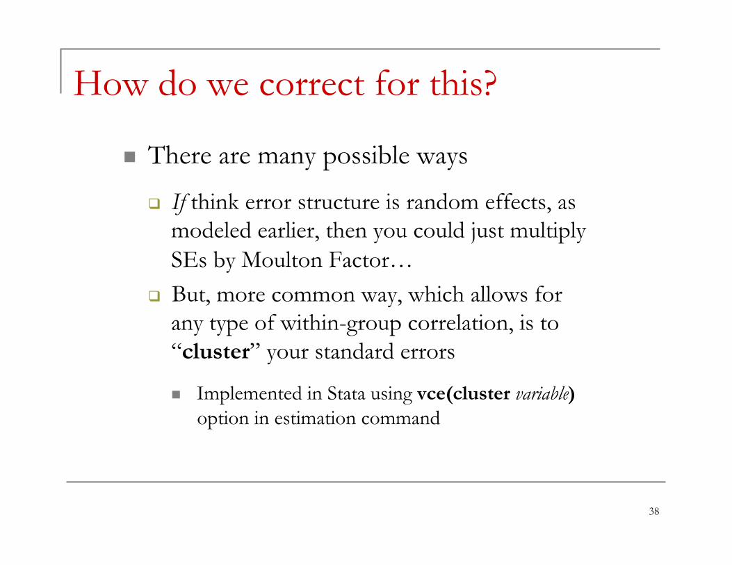
n  There are many possible ways

q  If think error structure is random effects, as modeled earlier, then you could just multiply SEs by Moulton Factor…

q  But, more common way, which allows for any type of within-group correlation, is to “cluster” your standard errors

n  Implemented in Stata using vce(cluster variable) option in estimation command

How do we correct for this?

38

n  Basic idea is that it allows for any type of correlation of errors within group

q  E.g. if “cluster” was a firm’s observations for years 1, 2, …, T, then it would allow corr(ui1, ui2) to be different than corr(ui1, ui3)

n  Moultan factor approach would assume these are all the same which may be wrong

n  Then, use independence across groups and asymptotics to estimate SEs

Clustered Standard Errors

39

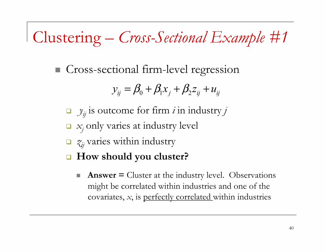
n  Cross-sectional firm-level regression

q  yij is outcome for firm i in industry j q  xj only varies at industry level q  zij varies within industry q  How should you cluster?

n  Answer = Cluster at the industry level. Observations might be correlated within industries and one of the covariates, x, is perfectly correlated within industries

Clustering – Cross-Sectional Example #1

40

0 1 2ij j ij ijy x z uβ β β= + + +

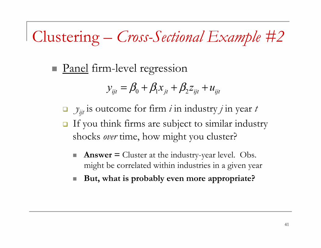
n  Panel firm-level regression

q  yijt is outcome for firm i in industry j in year t q  If you think firms are subject to similar industry

shocks over time, how might you cluster?

n  Answer = Cluster at the industry-year level. Obs. might be correlated within industries in a given year

n  But, what is probably even more appropriate?

Clustering – Cross-Sectional Example #2

41

0 1 2ijt jt ijt ijty x z uβ β β= + + +

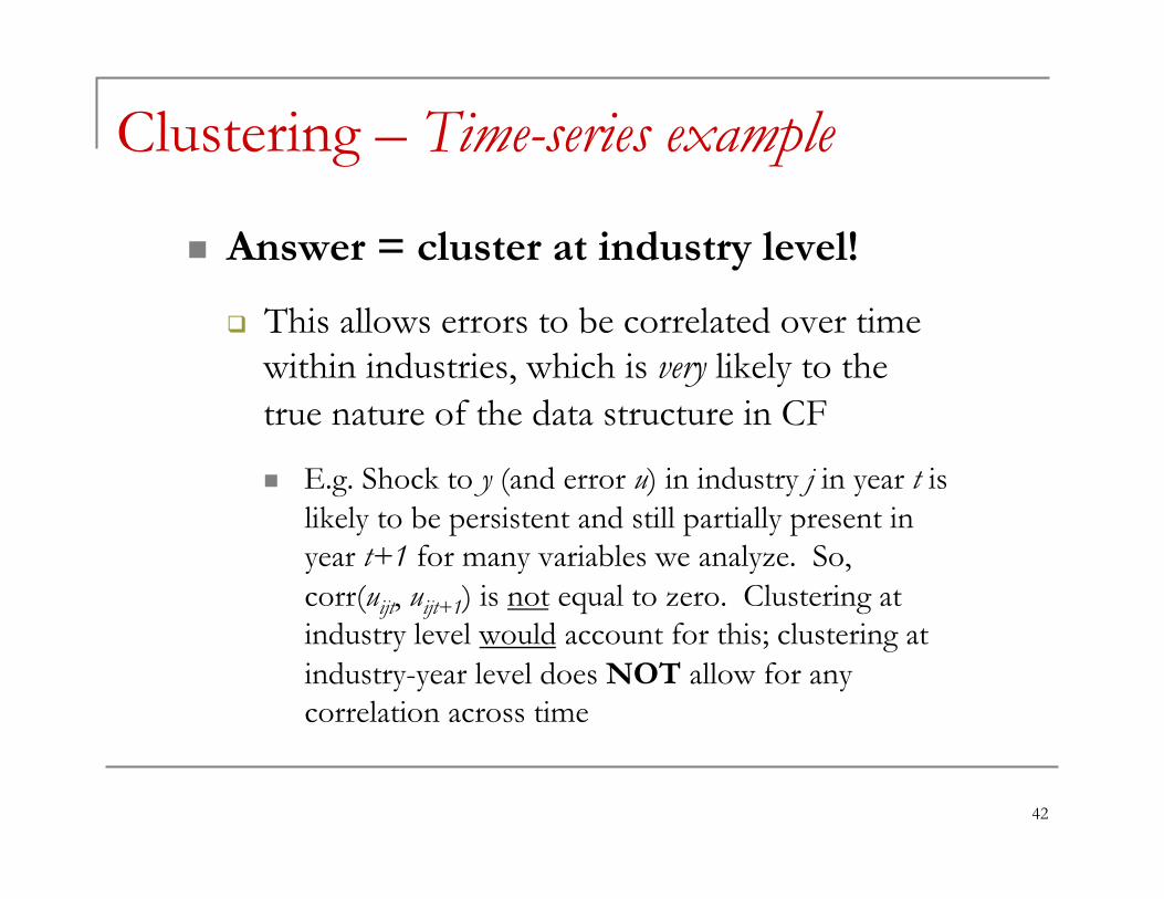
n  Answer = cluster at industry level!

q  This allows errors to be correlated over time within industries, which is very likely to the true nature of the data structure in CF

n  E.g. Shock to y (and error u) in industry j in year t is likely to be persistent and still partially present in year t+1 for many variables we analyze. So, corr(uijt, uijt+1) is not equal to zero. Clustering at industry level would account for this; clustering at industry-year level does NOT allow for any correlation across time

Clustering – Time-series example

42

n  Such time-series correlation is very common in corporate finance

q  E.g. leverage, size, etc. are all persistent over time q  Clustering at industry, firm, or state level is a non-

parametric and robust way to account for this!

Time-series correlation

43

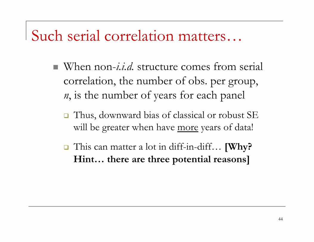
n  When non-i.i.d. structure comes from serial correlation, the number of obs. per group, n, is the number of years for each panel

q  Thus, downward bias of classical or robust SE will be greater when have more years of data!

q  This can matter a lot in diff-in-diff… [Why? Hint… there are three potential reasons]

Such serial correlation matters…

44

n  Serial correlation is particularly important in difference-in-differences because…

#1 – Treatment indicator is highly correlated over time! [E.g. for untreated firms is stays zero entire time, and for treated firms it stays equal to 1 after treatment]

#2 – We often have multiple pre- and post-treatment observations [i.e. many observations per group]

#3 – And, dependent variables typically used often have a high time-series dependence to them

Serial correlation in diff-in-diff [Part 1]

45

n  Bertrand, Duflo, and Mullainathan (QJE 2004) shows how bad this SE bias can be…

q  In standard type of diff-in-diff where true β=0, you’ll find significant effect at 5% level in as much as 45 percent of the cases!

n  Remember… you should only reject null hypothesis 5% of time when the true effect is actually zero!

Serial correlation in diff-in-diff [Part 2]

46

n  Whether to use both FE and clustering often causes confusion for researchers

q  E.g. should you have both firm FE and clustering at firm level, and if so, what is it doing?

Easiest to understand why both might be appropriate with a few quick questions…

Firm FE vs. firm clusters

47

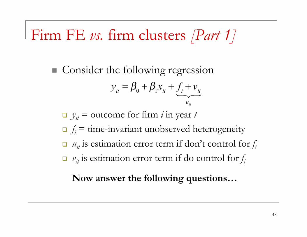
n  Consider the following regression

q  yit = outcome for firm i in year t q  fi = time-invariant unobserved heterogeneity q  uit is estimation error term if don’t control for fi q  vit is estimation error term if do control for fi

Now answer the following questions…

Firm FE vs. firm clusters [Part 1]

48

yit = β0 + β1xit + fi + vit

uit

!"#

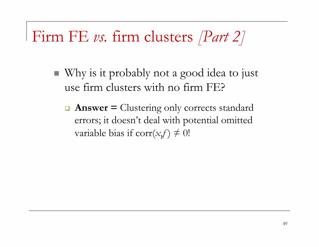
n  Why is it probably not a good idea to just use firm clusters with no firm FE?

q  Answer = Clustering only corrects standard errors; it doesn’t deal with potential omitted variable bias if corr(x,f ) ≠ 0!


49

n  Why should we still cluster at firm level if even if we already have firm FE?

q  Answer = Firm FE removes time-invariant heterogeneity, fi, from error term, but it doesn’t account for possible serial correlation!

n  I.e. vit might still be correlated with vit-1, vit-2, etc.

n  E.g. firm might get hit by shock in year t, and effect of that shock only slowly fades over time


50

n  Will we get consistent estimates with both firm FE and firm clusters if serial dependence in error is driven by time-varying omitted variable that is correlated with x?

q  Answer = No!

n  Clustering only corrects SEs; it doesn’t deal with potential bias in estimates because of an omitted variable problem!

n  And, Firm FE isn’t sufficient in this case either because omitted variable isn’t time-invariant


51

n  Cluster at most aggregate level of variation in your covariates

q  E.g. if one of your covariates only varies at industry or state level, cluster at that level

n  Always assume serial correlation

q  Don’t cluster at state-year, industry-year, firm-year; cluster at state, industry, or firm [this is particularly true in diff-in-diff]

Clustering – Practical Advice [Part 1]

52

n  Clustering is not a substitute for FE

q  Should use both FE to control for unobserved heterogeneity across groups and clustered SE to account for remaining serial correlation in y

n  Be careful when # of clusters is small…

Clustering – Practical Advice [Part 2]

53






54

n  Asymptotic consistency of estimated clustered standard errors depends on # of clusters, not # of observations

q  I.e. only guaranteed to get precise estimate of correct SE if we have a lot of clusters

q  If too few clusters, SE will be too low!

n  This leads to practical questions like… “If I do firm-level panel regression with 50 states and cluster at state level, are there enough clusters?”

Need enough clusters…

55

n  Unclear, but probably not a big problem

q  Simulations of Bertrand, et al (QJE 2004) suggest 50 clusters was plenty in their setting

n  In fact, bias wasn’t that bad with 10 states

n  This is consistent with Hansen (JoE 2007), which finds that 10 clusters is enough when using clusters to account for serial correlation

q  But, can’t guarantee this is always true, particularly in cross-sectional settings

How important is this in practice?

56

n  You can try aggregating the data to remove time-series variation

q  E.g. in diff-in-diff, you would collapse data into one pre- and one post-treatment observation for each firm, state, or industry [depending on what level you think is non-i.i.d], and then run the estimation

n  See Bertrand, Duflo, and Mullainathan (QJE 2004) for more details on how to do this

If worried about # of clusters…

57

n  Can have very low power

q  Even if true β≠0, aggregating approach can often fail to reject the null hypothesis

n  Not as straightforward (but still doable) when have multiple events at different times or additional covariates

q  See Bertrand, et al (QJE 2004) for details

Cautionary Note on aggregating

58

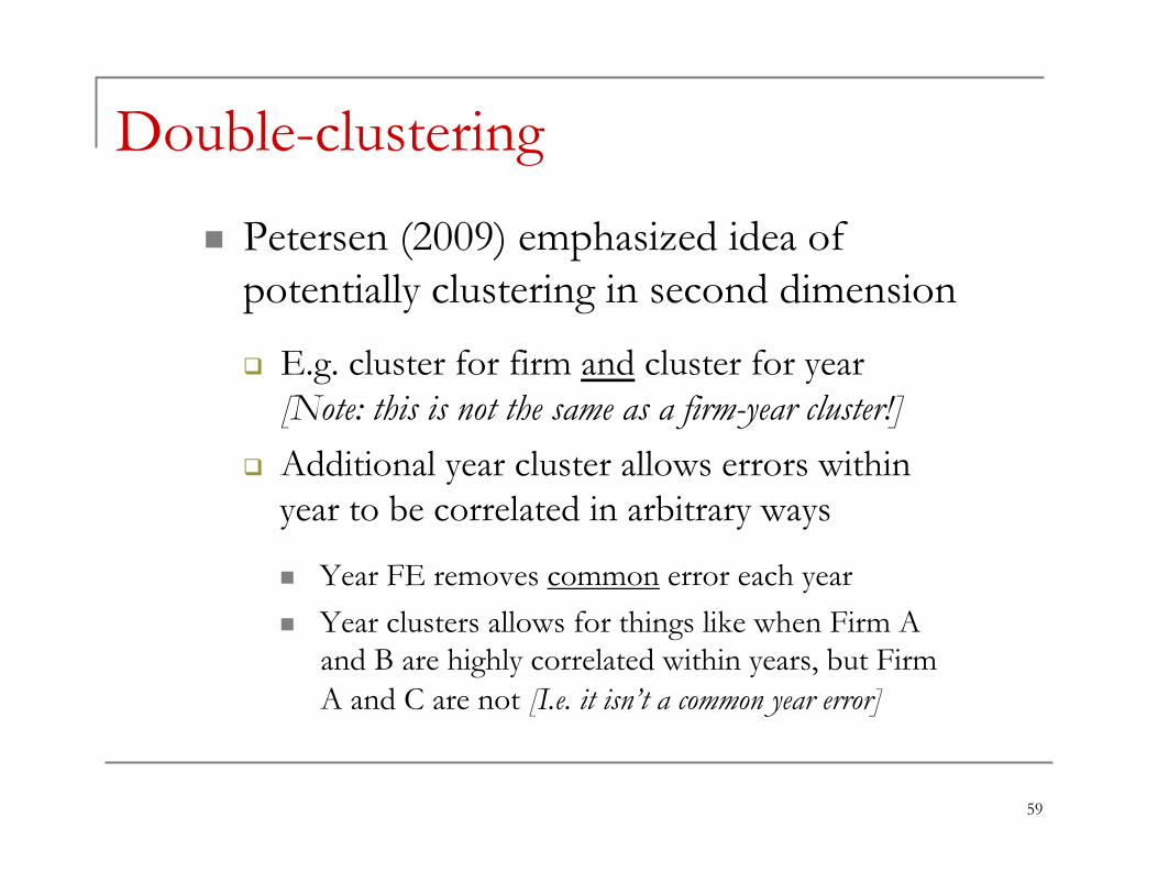
n  Petersen (2009) emphasized idea of potentially clustering in second dimension

q  E.g. cluster for firm and cluster for year [Note: this is not the same as a firm-year cluster!]

q  Additional year cluster allows errors within year to be correlated in arbitrary ways

n  Year FE removes common error each year n  Year clusters allows for things like when Firm A

and B are highly correlated within years, but Firm A and C are not [I.e. it isn’t a common year error]

Double-clustering

59

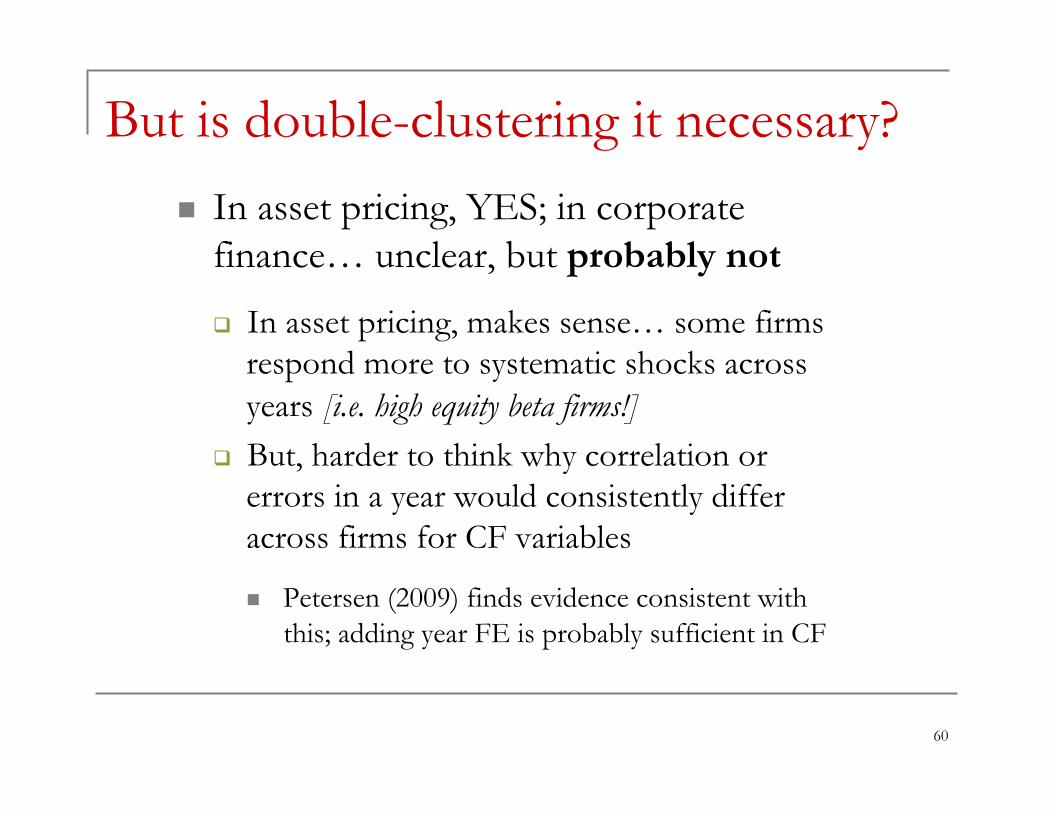
n  In asset pricing, YES; in corporate finance… unclear, but probably not

q  In asset pricing, makes sense… some firms respond more to systematic shocks across years [i.e. high equity beta firms!]

q  But, harder to think why correlation or errors in a year would consistently differ across firms for CF variables

n  Petersen (2009) finds evidence consistent with this; adding year FE is probably sufficient in CF

But is double-clustering it necessary?

60

Clustering in Panels – More Advice

n  Within Stata, two commands can do the fixed effects estimation for you

q  xtreg, fe q  areg

n  They are identical, except when it comes to the cluster-robust standard errors

q  xtreg, fe cluster-robust SE are smaller because it doesn’t adjust doF when clustering!

61

Clustering – xtreg, fe versus areg

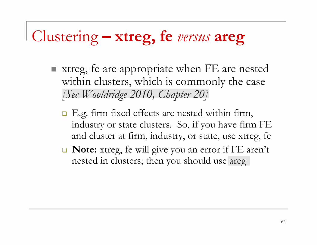
n  xtreg, fe are appropriate when FE are nested within clusters, which is commonly the case [See Wooldridge 2010, Chapter 20]

q  E.g. firm fixed effects are nested within firm, industry or state clusters. So, if you have firm FE and cluster at firm, industry, or state, use xtreg, fe

q  Note: xtreg, fe will give you an error if FE aren’t nested in clusters; then you should use areg

62





63

Limited dependent variables (LDV)

n  LDV occurs whenever outcome y is zero-one indicator or non-negative

q  If think about it, it is very common

n  Firm-level indicator for issuing equity, doing acquisition, paying dividend, etc.

n  Manager’s salary [b/c it is non-negative]

q  Zero-one outcomes are also called discrete choice models

64

Common misperception about LDVs

n  It is often thought that LDVs shouldn’t be estimated with OLS

q  I.e. can’t get causal effect with OLS q  Instead, people argue you need to use

estimators like Probit, Logit, or Tobit

n  But, this is wrong! To see this, let’s compare linear probability model to Probit & Logit

65

Linear probability model (LPM)

n  LPM is when you use OLS to estimate model where outcome, y, is an indicator

q  Intuitive and very few assumptions q  But admittedly, there are issues…

n  Predicted values can be outside [0,1] n  Error will be heteroskedastic [Does this cause bias?]

Answer = No! Just need to correct SEs

66

Logit & Probit [Part 1]

n  Basically, they assume latent model

q  y* is unobserved latent variable q  And, we assume observed outcome, y,

equals 1 if y*>0, and zero otherwise q  And, make assumption about error, u

n  Probit assumes u distributed normally n  Logit assumes u is logistic distribution

67

* 'y x uβ= +

x‘ is vector of controls, including constant

What are Logit & Probit? [Part 2]

n  With those assumptions, can show…

q  Prob(y* > 0|x) = Prob(u < x’β|x) = F(x’ β) q  And, thus Prob(y = 1|x) = F(x’ β), where F(x’ β) is cumulative distribution function of u

n  Because this is nonlinear, we use maximum likelihood estimator to estimate β

q  See Greene, Section 17.3 for details

68

What are Logit & Probit? [Part 3]

n  Note: reported estimates in Stata are not marginal effects of interest!

q  I.e. you can’t easily interpret them or compare them to what you’d get with LPM

q  Need to use post-estimation command “margins” to get marginal effects at average x

69

Logit, Probit versus LPM

n  Benefits of Logit & Probit

q  Predicted probabilities from Logit & Probit will be between 0 and 1…

n  But, are they needed to estimate casual effect of some random treatment, d?

70

NO! LPM is okay to use

n  Just think back to natural experiments, where treatment, d, is exogenously assigned

q  Difference-in-differences estimators were shown to estimate average treatment effects

q  Nothing in those proofs required assumption that outcome y is continuous with full support!

n  Same is true of non-negative y [I.e. Using Tobit isn’t necessary either]

71

Instrumental variables and LDV

n  Prior conclusions also hold in 2SLS estimations with exogenous instrument

q  2SLS still estimates local average treatment effect with limited dependent variables

72

Caveat – Treatment with covariates

n  There is, however, an issue when estimating treatment effects when including other covariates

q  CEF almost certainly won’t be linear if there are additional covariates, x

n  It is linear if just have treatment, d, and no X’s

n  But, Angrist-Pischke say not to worry…

73

Angrist-Pischke view on OLS [Part 1]

n  OLS still gives best linear approx. of CEF under less restrictive assumptions q  If non-linear CEF has causal interpretation, then

OLS estimate has causal interpretation as well q  If assumptions about distribution of error are

correct, non-linear models (e.g. Logit, Probit, and Tobit) basically just provide efficiency gain

74


n  But this efficiency gain (from using something like Probit or Logit) comes with cost…

q  Assumptions of Probit, Logit, and Tobit are not testable [can’t observe u]

q  Theory gives little guidance on right assumption, and if assumption wrong, estimates biased!

75


n  Lastly, in practice, marginal effects from Probit, Logit, etc. will be similar to OLS q  True even when average y is close to either 0 or 1

(i.e. there are a lot of zeros or lot of ones)

76

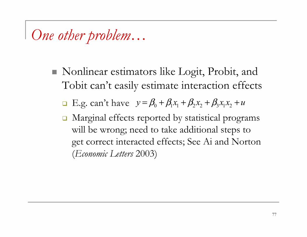
One other problem…

n  Nonlinear estimators like Logit, Probit, and Tobit can’t easily estimate interaction effects

q  E.g. can’t have q  Marginal effects reported by statistical programs

will be wrong; need to take additional steps to get correct interacted effects; See Ai and Norton (Economic Letters 2003)

77

0 1 1 2 2 3 1 2y x x x x uβ β β β= + + + +

One last thing to mention…

n  With non-negative outcome y and random treatment indicator, d

q  OLS still correctly estimates ATE q  But, don’t condition on y > 0 when selecting

your sample; that messes things up!

n  This is equivalent to “bad control” in that you’re implicitly controlling for whether y > 0, which is also outcome of treatment!

n  See Angrist-Pischke, pages 99-100

78

Summary of Today [Part 1]

n  Getting your SEs correct is important

q  If clustering isn’t important, run both “classical” and “robust” SE; choose higher

q  But, use clustering when…

n  One of key independent variables only varies at aggregate level (e.g. industry, state, etc)

n  Or, dependent variable or independent variables likely exhibit time series dependence

79


n  Miscellaneous advice on clustering

q  Best to assume time series dependence; e.g. cluster at group level, not group-year

q  Firm FE and firm clusters are not substitutes q  Use clustered SE produced by xtreg not areg

80


n  Can use OLS with LDVs

q  Still gives ATE when estimating treatment effect q  In other settings (i.e. have more covariates), still

gives best linear approx. of non-linear causal CEF

n  Estimators like Probit, Logit, Tobit have their own problems

81

In First Half of Next Class

n  Randomized experiments

q  Benefits… q  Limitations

n  Related readings; see syllabus

82

In Second Half of Next Class

n  Papers are not necessarily connected to today’s lecture on standard errors

83

Assign papers for next week…

n  Heider and Ljungqvist (JFE Forthcoming)

q  Capital structure and taxes

n  Iliev (JF 2010)

q  Effect of SOX on accounting costs

n  Appel, Gormley, Keim (working paper, 2015)

q  Impact of passive investors on governance

84

Break Time

n  Let’s take our 10 minute break n  We’ll do presentations when we get back

85

fnce 926 empirical methods in cffnce 926 empirical methods in cf professor todd gormley lecture 11...

Documents