fluid mechanics - mtf053 - lecture 7

Fluid Mechanics - MTF053

Lecture 7

Niklas Andersson

Chalmers University of Technology

Department of Mechanics and Maritime Sciences

Division of Fluid Mechanics

Gothenburg, Sweden

[email protected]

mailto:[email protected]

Chapter 4 - Differential Relations for Fluid Flow

Overview

Fluid Dynamics

Basic

Concepts

Pressure

hydrostatic

forces

buoyancy

Fluid Flow

velocity

field

Reynolds

number

flow

regimes

Thermo-

dynamics

pressure,

density,

and tem-

perature

state

relations

speed of

sound

entropy

Fluid

fluid

conceptcontinuum

viscosity

Fluid Flow

Com-

pressible

Flow

shock-

expansion

theory

nozzle

flow

normal

shocks

speed of

sound

External

Flow

separation turbulence

boundary

layer

Reynolds

number

Duct Flow

friction

and losses

turbulent

flow

laminar

flow

flow

regimes

Turbulence

Turbulence

Modeling

Turbulence

viscosity

Reynolds

stressesReynolds

decom-

position

Flow

Relations

Dimen-

sional

Analysis

modeling

and

similarity

nondi-

mensional

equations

The Pi

theorem

Differential

Relations

rotation

stream

function

conser-

vation

relations

Integral

Relations

Bernoulli

conser-

vation

relations

Reynolds

transport

theorem

Learning Outcomes

4 Be able to categorize a flow and have knowledge about how to select

applicable methods for the analysis of a specific flow based on category

14 Derive the continuity, momentum and energy equations on differential form

36 Define and explain vorticity

let’s push the control volume approach to the limit ...

Niklas Andersson - Chalmers 4 / 49

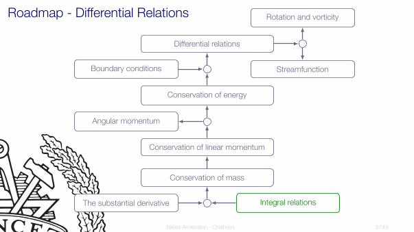
Roadmap - Differential Relations

Differential relations

Conservation of energy

Conservation of linear momentum

Conservation of mass

The substantial derivative Integral relations

Angular momentum

Boundary conditions

Rotation and vorticity

Streamfunction


Differential Relations

seeking the point-by-point details of a flow pattern by analyzing an

infinitesimal region of the flow


Differential Relations

I Apply the four basic conservation laws to an infinitesimally small control volume

I The differential relations are in general very difficult to solve

I analytical solutions exists for a few cases

I The differential relations form the basis for CFD software


High-Speed Nozzle Flow


The Acoustic Signature of a Supersonic Jet

Screeching rectangular supersonic jet


Lots of Equations Ahead








Angular momentum

Boundary conditions


Streamfunction


Frame of Reference

Eulerian: observer fixed in space

Lagrangian: observer follows a fluid particle

recall the speedometer/traffic-camera analogy


Acceleration Field

In order to get to Newton’s second law, we need the acceleration vector

Velocity field:

V(r, t) = exu(x, y, z, t) + eyv(x, y, z, t) + ezw(x, y, z, t)

Acceleration field:

a =dVdt

= ex

du

dt+ ey

dv

dt+ ez

dw

dt


Acceleration Field

Each scalar component of the velocity vector (u, v,w) is a function of four variables(x, y, z, t) and thus

du(x, y, z, t)

dt=

∂u

∂t+

∂u

∂x

dx

dt+

∂u

∂y

dy

dt+

∂u

∂z

dz

dt

By definition dx/dt = u, dy/dt = v, and dz/dt = w

du(x, y, z, t)

dt=

∂u

∂t+ u

∂u

∂x+ v

∂u

∂y+w

∂u

∂z=

∂u

∂t+ (V · ∇)u


Acceleration Field

ax =∂u

∂t+ u

∂u

∂x+ v

∂u

∂y+w

∂u

∂z=

∂u

∂t+ (V · ∇)u

ay =∂v

∂t+ u

∂v

∂x+ v

∂v

∂y+w

∂v

∂z=

∂v

∂t+ (V · ∇)v

az =∂w

∂t+ u

∂w

∂x+ v

∂w

∂y+w

∂w

∂z=

∂w

∂t+ (V · ∇)w

a =∂V∂t︸︷︷︸local

+

(u∂V∂x

+ v∂V∂y

+w∂V∂z

)︸︷︷︸

convective

=∂V∂t

+ (V · ∇)V =DVDt


Acceleration Field

a =∂V∂t︸︷︷︸local

+

(u∂V∂x

+ v∂V∂y

+w∂V∂z

)︸︷︷︸

convective

=∂V∂t

+ (V · ∇)V =DVDt

local acceleration: only in unsteady flows

convective acceleration: fluid particle that moves through regions of spatiallyvarying velocity

I nozzle flowI diffuser flow


Substantial derivative

I The total temporal derivative

I the sum of the local derivative and the convective derivativeI often referred to as the substantial derivative

I The substantial derivative follows a fluid particle but is expressed in an Eulerian

frame of reference

The substantial derivative is an operator that can be applied to any variable

Dp

Dt=

∂p

∂t+ u

∂p

∂x+ v

∂p

∂y+w

∂p

∂z=

∂p

∂t+ (V · ∇)p








Angular momentum

Boundary conditions


Streamfunction


Mass Conservation y

x

z

(ρu +

∂

∂x(ρu)dx

)dydzρudydz

dx

dy

dz

ˆCV

∂ρ

∂tdV +

∑i

(ρiAiVi)out −∑i

(ρiAiVi)in = 0

ˆCV

∂ρ

∂tdV ≈ ∂ρ

∂tdxdydz

∂ρ

∂tdxdydz +

∂

∂x(ρu)dxdydz +

∂

∂y(ρv)dxdydz +

∂

∂z(ρw)dxdydz = 0


Mass Conservation

The result is the continuity equation - conservation of mass for an infinitesimal control

volume

∂ρ

∂t+

∂

∂x(ρu) +

∂

∂y(ρv) +

∂

∂z(ρw) = 0

or in more compact form using vector notation

∂ρ

∂t+∇ · (ρV) = 0

Incompressible flow (constant density)

∂u

∂x+

∂v

∂y+

∂w

∂z= ∇ · V = 0








Angular momentum

Boundary conditions


Streamfunction


Linear Momentum

∑F =

ˆCV

∂

∂t(Vρ)dV +

∑(miVi)out −

∑(miVi)in

∂

∂t(Vρ)dV ≈ ∂

∂t(Vρ)dxdydz


Linear Momentum y

x

z

(ρuV +

∂

∂x(ρuV)dx

)dydzρuVdydz

dx

dy

dz

Face Inlet momentum flux Outlet momentum flux

x ρuVdydz

[ρuV +

∂

∂x(ρuV)dx

]dydz

y ρvVdxdz

[ρvV +

∂

∂y(ρvV)dy

]dxdz

z ρwVdxdy

[ρwV +

∂

∂z(ρwV)dz

]dxdy


Linear Momentum

∑F =

[∂

∂t(Vρ) +

∂

∂x(ρuV) +

∂

∂y(ρvV) +

∂

∂z(ρwV)

]dxdydz


Linear Momentum

∂

∂t(Vρ)︸︷︷︸

V ∂ρ∂t

+ρ ∂V∂t

+∂

∂x(ρuV)︸︷︷︸

V ∂∂x

(ρu)+ρu ∂V∂x

+∂

∂y(ρvV)︸︷︷︸

V ∂∂y

(ρv)+ρv ∂V∂y

+∂

∂z(ρwV)︸︷︷︸

V ∂∂z

(ρw)+ρw ∂V∂z

can be rewritten as

V[∂ρ

∂t+∇ · (ρV)

]︸︷︷︸continuity equation

+ρ

(∂V∂t

+ u∂V∂x

+ v∂V∂y

+w∂V∂z

)︸︷︷︸

∂V∂t

+(V·∇)V=DVDt

and thus ∑F = ρ

DVDt

dxdydz


Linear Momentum - Forces

∑F = ρ

DVDt

dxdydz

∑F :

body forces: gravity and other field forces

surface forces: pressure and viscous stresses


Linear Momentum - Gravity Force

dFgravity = ρgdxdydz

if gravity is aligned with the negative z-direction

dFgravity = −ezρgdxdydz


Linear Momentum - Surface Forces

y

x

zdx

dy

dz

σyy

σyxσyz

σzx

σzy

σzz

σxy

σxz σxxσij =

∣∣∣∣∣∣−p+ τxx τyx τzx

τxy −p+ τyy τzyτxz τyz −p+ τzz

∣∣∣∣∣∣



y

x

z

(σxx +

∂σxx

∂xdx

)dydz

σzxdxdy

σyxdxdz

σxxdydz

(σzx +

∂σzx

∂zdz

)dxdy

(σyx +

∂σyx

∂ydy

)dxdz

dx

dy

dz

dFx,surf =

[∂

∂x(σxx) +

∂

∂y(σyx) +

∂

∂z(σzx)

]dxdydz



dFx,surf =

[∂

∂x(σxx) +

∂

∂y(σyx) +

∂

∂z(σzx)

]dxdydz

σxx = τxx − p, σyx = τyx, σzx = τzx

dFx,surf =

[−∂p

∂x+

∂

∂x(τxx) +

∂

∂y(τyx) +

∂

∂z(τzx)

]dxdydz



dFx,surf =

[−∂p

∂x+

∂

∂x(τxx) +

∂

∂y(τyx) +

∂

∂z(τzx)

]dxdydz

dFy,surf =

[−∂p

∂y+

∂

∂x(τxy) +

∂

∂y(τyy) +

∂

∂z(τzy)

]dxdydz

dFz,surf =

[−∂p

∂z+

∂

∂x(τxz) +

∂

∂y(τyz) +

∂

∂z(τzz)

]dxdydz



dF =[−∇p+∇ · τij

]dxdydz

where

τij =

∣∣∣∣∣∣τxx τyx τzxτxy τyy τzyτxz τyz τzz

∣∣∣∣∣∣is the viscous stress tensor


Linear Momentum - Forces

Now, inserting the forces into the momentum equation gives

ρg −∇p+∇ · τij = ρDVDt


Linear Momentum

vector notation is powerfull, tensor notation is even better ...

ρgx −∂p

∂x+

∂τxx∂x

+∂τyx∂y

+∂τzx∂z

= ρ

(∂u

∂t+ u

∂u

∂x+ v

∂u

∂y+w

∂u

∂z

)

ρgy −∂p

∂y+

∂τxy∂x

+∂τyy∂y

+∂τzy∂z

= ρ

(∂v

∂t+ u

∂v

∂x+ v

∂v

∂y+w

∂v

∂z

)

ρgz −∂p

∂z+

∂τxz∂x

+∂τyz∂y

+∂τzz∂z

= ρ

(∂w

∂t+ u

∂w

∂x+ v

∂w

∂y+w

∂w

∂z

)

Note! the convective term (RHS) is nonlinear


Linear Momentum

Recall:

”For a Newonian fluid, the viscous stresses are proportional to the element

strain and the viscosity”

For incompressible flow:

τxx = 2µ∂u

∂x, τyy = 2µ

∂v

∂y, τzz = 2µ

∂w

∂z

τxy = τyx = µ

(∂u

∂y+

∂v

∂x

), τxz = τzx = µ

(∂u

∂z+

∂w

∂x

)

τyz = τzy = µ

(∂v

∂z+

∂w

∂y

)Niklas Andersson - Chalmers 35 / 49

Linear Momentum

ρDu

Dt= ρgx −

∂p

∂x+ µ

(∂2u

∂x2+

∂2u

∂y2+

∂2u

∂z2

)

ρDv

Dt= ρgy −

∂p

∂y+ µ

(∂2v

∂x2+

∂2v

∂y2+

∂2v

∂z2

)

ρDw

Dt= ρgz −

∂p

∂z+ µ

(∂2w

∂x2+

∂2w

∂y2+

∂2w

∂z2

)

The incompressible Navier-Stokes equations


Linear Momentum

I Non-linear equations

I Three equations and four unknowns (p, u, v,w)

I Combined with the continuity equations we have four equations and four

unknowns

The incompressible Navier-Stokes equations


Example - Coutette Flow

y = −h

y = h

y

x

u(y)

fixed wall

V

I incompressible (ρ = const)

I steady-state

I lower plate fixed, upper plate moving with the velocity V

I flow only in the x-direction v = w = 0, u 6= 0

I no pressure gradient



continuity:

∂u

∂x+

∂v

∂y+

∂w

∂z= 0 ⇒ {v = w = 0} ⇒ ∂u

∂x= 0

momentum equation (x-direction):

ρ

(u∂u

∂x+ v

∂u

∂y

)= −∂p

∂x+ρgx+µ

(∂2u

∂x2+

∂2u

∂y2

)⇒ {v = w = 0,

∂p

∂x= 0} ⇒ µ

∂2u

∂y2= 0



∂2u

∂y2= 0 ⇒ u = ay + b

boundary conditions:

u(h) = V

u(−h) = 0

}⇒

V = ah + b

+ 0 = −ah + b

V = 2b

b =V

2

V = ah + b

− 0 = −ah + b

V = 2ah

a =V

2h



y = −h

y = h

y

x

u(y)

fixed wall

V

u =V

2

(yh− 1

)


Example - Poiseuille Flow

y = −h

y = h

y

x

u(y)

umax

fixed wall

fixed wall

I incompressible (ρ = const)

I steady-state

I lower and upper plate fixed

I flow only in the x-direction v = w = 0, u 6= 0

I pressure gradient driven



continuity:

∂u

∂x+

∂v

∂y+

∂w

∂z= 0 ⇒ {v = w = 0} ⇒ ∂u

∂x= 0

momentum equation (x-direction):

ρ

(u∂u

∂x+ v

∂u

∂y

)= −∂p

∂x+ ρgx + µ

(∂2u

∂x2+

∂2u

∂y2

)⇒ {v = w = 0} ⇒ µ

∂2u

∂y2=

∂p

∂x



momentum equation (y-direction and z-direction):

∂p

∂y= 0

∂p

∂z= 0

⇒ p = p(x)



µd2u

dy2=

dp

dx= const < 0

I Why constant?

I RHS function of x onlyI LHS function of y onlyI RHS=LHS ⇒ must be a constant

I Why < 0?I pressure must decrease in the flow direction



µd2u

dy2=

dp

dx= const < 0

u =1

2µ

dp

dxy2 + ay + b



boundary conditions:

u(h) = 0u(−h) = 0

}⇒

0 =1

2µ

dp

dxh2 + ah + b

+ 0 =1

2µ

dp

dxh2 − ah + b

0 =1

µ

dp

dxh2 + 2b

b = − 1

2µ

dp

dxh2

0 =1

2µ

dp

dxh2 + ah + b

− 0 =1

2µ

dp

dxh2 − ah + b

0 = 2ah

a = 0



y = −h

y = h

y

x

u(y)

umax

fixed wall

fixed wall

u = − h2

2µ

dp

dx

(1−

(yh

)2)

du

dy=

dp

dx

y

µ⇒ du

dy

∣∣∣∣y=0

= 0 ⇒ umax = u(0) = −dp

dx

h2

2µ

(remember: dp/dx < 0)Niklas Andersson - Chalmers 49 / 49

fluid mechanics - mtf053 - lecture 7

Documents