SCA 2001-06

1

FLOW IMAGING IN CORE SAMPLES BY ELECTRICALIMPEDANCE TOMOGRAPHY

J.J.A. van Weereld (1), M.A. Player (2), D.A.L. Collie (3), A.P. Watkins (3), D. Olsen (4)

(1) Geolink, Aberdeen (2) Department of Engineering, University of Aberdeen, Scotland(3) Robertson Research International Ltd., Aberdeen (4) Geological Survey of Denmark

and Greenland, Copenhagen, Denmark

ABSTRACT3D Electrical Impedance Tomography (EIT) provides in-situ, steady or unsteady state,imaging of fluid distribution in core samples at reservoir pressures. Although spatialresolution is not able to match that obtained through x-ray CT or MRI, the techniqueprovides an inexpensive, simple, practical and safe means of monitoring the resistivitydistribution of reservoir fluids in a 38 mm core plug, in near real-time and in full 3D.

An array of 192 electrodes carried on a flexible printed circuit is wrapped around a coreplug mounted in a Hassler or Hoek-type core holder. A fast bipolar current pulse allows a4-wire type resistance measurement on all electrodes around the surface of the coresample. A data set is thus generated that embodies the 3D resistivity/conductivity profile ofthe whole sample as a transresistance matrix. Processing of these measurementsreconstructs the full 3D internal resistivity distribution, and correspondingly thedistribution of conducting fluids in the sample.

The iterative reconstruction algorithm utilises a Finite Element forward model, for thecylindrical core plug, comprising 1080 triangular prismatic linear Galerkin elements.Regularised Jacobian and Hessian matrices of the non-linear inverse problem areconstructed, and inversion uses Levenberg-Marquardt and truncated-Newton algorithms,implemented in MATLAB.

The real-time capability of EIT data acquisition permits imaging and analysis of the two-phase saturation system, including flow-front monitoring, characterisation of the flowregime, the distribution of residual oil or water at the final stages of relative permeabilitytests, and capillary end effects. Initial laboratory tests demonstrate repeatability andreliability of results.

INTRODUCTIONCore analysis is concerned with the study of fluid-rock interactions in rock samplesobtained from hydrocarbon reservoirs. The samples are usually in the shape of cylinders,with a nominal diameter of 38 mm and a length of 50 mm. The fluids involved in thesestudies are crude or synthetic oil, and brine. In various static and dynamic experiments theresistance of the sample is measured, and the resistivity calculated. This can in turn berelated to fluid saturation [1].

SCA 2001-06

2

The two- or four-wire measurement is commonly made with a commercially availableLCR bridge with sinusoidal excitation. Problems exist with obtaining a satisfactory contactbetween the sample and the measurement electrodes, especially for samples with low watersaturation. The art involved in making the measurements involves the application of silverfilter discs or brine wetted tissue as contact materials, and choosing a measurementfrequency for minimum phase angle [2]. Nevertheless, if these problems can be controlled,the large difference in resistivity of the fluids involved suggests Electrical ImpedanceTomography (EIT) as an ideal method for imaging fluid distribution in the sample.

In EIT generally, and specifically here Electrical Resistance Tomography, an image ofresistivity (the specific resistance of the material, Ωm) throughout the volume of an objectis reconstructed from measurements of resistance (two- or four-wire voltage/current ratios,Ω) taken at the surface. This generates a non-linear, ill-posed inverse problem, because theresistivity distribution in the sample itself modifies the flow of current, and the sensitivityto changes in resistivity depends strongly on position within the sample [3]. In this respectthe method is more computationally demanding than x-ray tomography, where the inverseproblem is essentially linear. We have adopted a well-known reconstruction method forEIT, which uses iterative least squares to minimise the difference between finite element(FE) estimates of resistance and the actual measurements [3, 4, 5]. However, a directimplementation is particularly computationally intensive, requiring some variation to giveacceptable times for 3D reconstruction.

This paper describes our approaches to the measurement and algorithmic issues raised byEIT, and gives results for flow of oil and brine through sandstone samples. Derivation ofthe saturation distribution on a voxel (3D-pixel) by voxel basis should follow directlyusing pore structure information established from measurements on a fully water saturatedsample, and from sample petrographic parameters and brine resistivity. We expect this tobe the subject of further work.

RESISTANCE MEASUREMENTConsider a core to which N electrodes are attached. An individual resistance value isobtained by connecting a current generator to one pair of electrodes, and measuring voltagebetween another pair, and a dataset for an EIT reconstruction will in principle consist of allsuch measurements. However these are not all independent and, taking account ofreciprocity, the maximum number of independent measurements is ( )12

1 −NN . To obtain3D reconstructions, it is clear that electrodes should be spread fairly uniformly over thesurface of the sample, and it is also clear that in principle the resolution should rise withthe number of electrodes. We have used an array of 192 electrodes (8 rings of 24) placedon the circumference of the sample. This number is a compromise between resolution onone hand, and manufacturability of the electrode array and computing capacity for thereconstruction algorithm on the other.

SCA 2001-06

3

Each electrode in contact with the brine forms an electrochemical interface, which is wellunderstood [6]. In an electrical sense, the interface can be considered as a capacitor, Cd,usually referred to as the double layer capacitor, in parallel with a resistor Re, the latterbeing not necessarily linear (figure 1). The values of Re and Cd are dependent on electrodematerial, brine constituents, and applied potential. The electrode material determineswhether the system is reversible (i.e. if the chemical reaction on the electrode by an electriccurrent can be reversed by reversing the current), or irreversible. The latter is also referredto as a polarisable electrode. An example of the former is a silver-silver chloride electrode,an example of the latter gold or platinum. For a reversible electrode its behaviour ispredominantly governed by Re, for the polarisable electrode by Cd. A frequent method fordealing with this situation is to use AC measurement, as in a single resistancedetermination. However this normally requires digitising the sinewave response over anumber of cycles, and compensating for the phase-shifts resulting from the variouscapacitances. We have instead used a “bipolar DC pulse” technique. Using thismeasurement method in combination with suitable multiplexing and control circuitry, adata acquisition system for impedance tomography has been successfully designed.

Figure 1. Electrode model.

For a four-wire DC measurement a stable current will have to be established in the subjectof interest, for the time it takes to make a voltage measurement to the required precision.During this time no irreversible process should take place: i.e. when the electrodes are of apolarisable kind, the voltage to which the double layer capacitance is charged by themeasurement current I, should remain below the voltage at which an electrochemicalreaction will take place. This determines the maximum value of the current pulse duration t(figure 2). The total net charge transported through the solution during the measurementshould be zero to avoid permanent changes to its properties. It follows that a pulse ofreversed current will have to be applied with an equal product It. The impedance of thevoltage measurement circuitry will be generally much larger than the electrode equivalent

SCA 2001-06

4

parallel resistance Re, and will therefore correctly measure the voltage generated by theconstant current over the unknown resistance Rx. The minimum duration of the currentpulse is determined by (i) the parallel parasitic capacitance CPc in the current electrodecircuitry in conjunction with the measurement current, (ii) the parallel parasitic capacitanceCPv in the voltage measurement circuitry in relation to the resistance of the medium Rx andRf, and to the aperture time of the A to D (analog-to-digital) converter used in themeasurement circuit.

The required application of a bipolar current pulse has an added benefit. The potentialdifference between electrode and solution (brine), which exists in every electrochemicalinterface, may not be the same for practical electrodes. This electrode offset Vos may becaused by concentration fluctuations in the solution, or property variations of the electrodematerial. If a voltage measurement is made during both positive and negative currentpulses, and the absolute values of the currents are the same, this offset voltage can becalculated and removed (figure 2). The same is true for offset voltages in the input circuitryfor the voltage measurement. Two-wire bipolar pulse conductivity measurements havepreviously been proposed for the measurement of chemical reaction rates [7, 8, 9], inwhich offset compensation was implemented in hardware.

(a)

(b)

(c)

0 t 2tTs Ts

VmP

Vos

0V

VmN

Figure 2. Waveforms for the “bipolar DC pulse” method.

The task of attaching 192 electrodes to the cylindrical surface of the sample has been maderelatively simple, by depositing the electrodes on a flexible printed circuit board (figure 3),which is then wrapped around the sample. The geometrical position of the electrodes onthe flexible circuit is fixed, which restricts the size of the sample to a length of 50 mm, anda diameter of 38 mm. The electrodes are electro-plated with the required electrode metal.The flexible circuit is a disposable item.

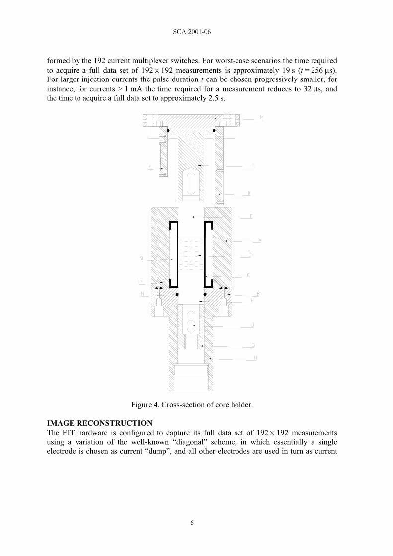
The assembly can be used in a Hassler or Hoek-type core holder (figure 4), as the part ofthe flexible circuit carrying the connections to the electrodes is brought out between theconfining sleeve [C] and the “fixed” platen [E]. Application of confining pressure [Q]

SCA 2001-06

5

ensures the electrodes are firmly in contact with the sample [D]. Proprietary constructionof the flexible printed circuit prevents any leakage between electrodes, or between circuitand platen where it exits the cell. The flexible circuit attaches to connectors [K] which arean integral part of the cell electronics (multiplexer), mounted on support plate [M]. Theplatens are manufactured from PEEK (poly aryl ether ether ketone) for electricalinsulation.

(a) (b)Figure 3. Flexible electrode array. (a) Layout of flexible printed circuit board: 8 × 24electrode array on the right, four connector pads at top and bottom. (b) Indication of

electrode layout and numbering when applied to core surface.

Electrically the system consists of three main components. All control circuitry isaccomodated on a single PC ISA bus card. Control signals are optically coupled to theanalog electronics and to the multiplexer, to prevent ground induced noise. The analogelectronics comprises current pulse generator and voltage measurement circuitry, and ishoused with its own linear power supply in a separate screened enclosure. The multiplexerconsists of electronic switches to select current and voltage electrodes and is mounteddirectly on the core holder, to keep the (high impedance) voltage path as short as possible.

The resolution for the voltage measurement is 16 bits. Depending on current levels andresistance values, tests on a single “dummy sample” simulating the circuit of figure 1 showstandard deviations of between 1 and 4 LSB’s. It is obviously more difficult to characterisecircuit performance on real samples, but comparisons between datasets suggest a similarlevel of variation. A limit on the speed of the data acquisition is imposed by the inputcapacitance of the current switch. If the sample has a relatively high resistivity, the use oflow currents is required to remain in the measurement range of the A to D converter. Theinput capacitance of the current switch is approximately 3.5 nF, the main part of which is

SCA 2001-06

6

formed by the 192 current multiplexer switches. For worst-case scenarios the time requiredto acquire a full data set of 192 × 192 measurements is approximately 19 s (t = 256 µs).For larger injection currents the pulse duration t can be chosen progressively smaller, forinstance, for currents > 1 mA the time required for a measurement reduces to 32 µs, andthe time to acquire a full data set to approximately 2.5 s.

Figure 4. Cross-section of core holder.

IMAGE RECONSTRUCTIONThe EIT hardware is configured to capture its full data set of 192 × 192 measurementsusing a variation of the well-known “diagonal” scheme, in which essentially a singleelectrode is chosen as current “dump”, and all other electrodes are used in turn as current

SCA 2001-06

7

sources. We used a scheme that numbers neighbouring electrodes along the axial directionconsecutively, choosing each axial row in turn and numbering always in the same direction(figure 3(b)). Current dump and voltage reference are then selected close together, usuallyon electrode ring 3 (approximately half way along the sample). Injection at all 192electrodes follows, with the measurement of the required 192 voltage measurements foreach injection. This pattern is repeated three more times for the reference pair locatedsimilarly but one quarter, one half and three quarters around the sample. Additionally, atleast one identical data set is captured immediately and compared to provide an assessmentof the reliability of the data.

The full data set is then recast as a transresistance matrix RT, which represents the dataindependently of the particular measurement scheme. We use a formulation for which thevoltage variables V are branch voltages between adjacent electrodes, and the currentvariables I are corresponding loop currents. Matrix elements represent the ratios of thesevalues for particular electrode pairs:

IRV T= (1)

This formulation has the advantage that most elements can be determined using only four-wire voltage and current measurements. Since R is symmetrical, this process reduces thevolume of data passed to the reconstruction algorithm.

A well-known reconstruction method uses iterative least squares to minimise the differencebetween Finite Element (FE) estimates of resistance and the actual measurements [3, 4, 5].The Levenberg-Marquardt algorithm [10] has been found particularly useful. It is a fullNewton approach, where each iteration step requires calculation and inversion of thesecond derivative of the cost function (Hessian matrix). Tikhonov regularisation, adding aquadratic smoothness constraint to the cost function, improves conditioning of theproblem, although it may bias the final image [5, 11]. The update equation of theregularised Levenberg-Marquardt method is [11]:

( ) ( )( ) kkFEEITT

kkT

k RRRJIRJJ ραρρεα −−=∆++ . (2)

Here ρk is the vector of resistivity values, at iteration k, and ∆ρ the resistivity update. REITand RFE are the measured and estimated transresistance matrices (reordered as vectors).The Jacobian matrix Jk expresses the derivative of the vector VFE with respect to ρk. R isthe regularisation matrix. Parameters α and ε control, respectively, levels of Tikhonov andof Levenberg-Marquardt regularisation. In implementing equation 2, the majorcomputational bottleneck is calculation of the product k

Tk JJ [4, 10]. This is particularly

important for true 3D geometry. To retain the basic, highly effective, structure of theLevenberg-Marquardt method, but to avoid a full matrix multiply, we have used atruncated-Newton (TN) algorithm in which solution of equation 2 is performed using the

SCA 2001-06

8

preconditioned conjugate gradient (PCG) algorithm [12]. The update at iteration i involvesthe Hessian matrix H only through the expression [13]

( ) ( ) iikT

ki pIRpJJq εα ++= (3)

the significance of which is that only matrix-vector multiplications are required. Theoverall cost of the solution then depends on the rate of PCG convergence. Convergence isimproved by preconditioning, which in effect multiplies H by an approximation to itsinverse. If elements of Jk with low absolute value are truncated to zero, the resulting sparseapproximation J(S)k provides a useful preconditioner:

IRJJM kST

kS εα ++= )()( (4)

at substantially lower cost than for the full product H. Behaviour of the outer Levenberg-Marquardt loop of this algorithm is controlled, as usual, by parameters α and ε, while theinner PCG loop is controlled by parameters that set the sparsity of J(S)k and the tolerance onPCG convergence. In practice, sparsity can be set so that adequate PCG convergence isobtained with around 10 iterations, and the time taken for the PCG solution is roughlyequal to the time taken to form (and factorise) M.

This algorithm requires an FE model to solve the forward problem, and to generate theJacobian J. Upright triangular prismatic elements are well suited geometrically to meshingof the cylindrical core, and also yield a relatively straightforward analytical form for the 6-node linear Galerkin local admittance matrix. (We have verified our own analyticalformulation by comparison with Pinheiro et al. [14].) However, decomposing each prisminto 3 tetrahedra, and averaging over the 6 possible decompositions, is found to give betteraccuracy. The 3D solutions generated by this forward model are closer to actual measuredresults than those from 2D calculations as commonly used in EIT. This is not surprising inview of the highly artificial assumption, inherent in the 2D models, that current flow isrestricted to planes [5, 10]. Delaunay triangulation is used to generate the FE mesh.

Tests on the TN reconstruction scheme indicate acceleration by a factor of about 9,compared with direct multiplication to form the Hessian. For an FE mesh of 1080 elements(9 rings of 120 elements, equivalent to a spatial resolution of approximately 4×4×4 mm3)the time per iteration at optimum parameter settings is about 134 seconds on a 450MHzPC, and convergence to a final image typically requires 4 to 6 iterations. Accuracy ofrecovered resistivity in simulations, using realistic values of resistivity contrast, isgenerally within 5% over regions of fairly constant resistivity. Obviously, the localaccuracy falls in regions of high resistivity gradient, where the FE mesh cannot representthe resistivity correctly. However, there may also appear local anomalies due to operationof the algorithm. Modifying regularisation to a mixture of quadratic constraints onresistivity and conductivity is fairly effective at controlling these. On the other hand,accuracy rises for more uniform samples.

SCA 2001-06

9

RESULTS AND DISCUSSIONA view of the complete system, assembled on the sample holder, is shown in figure 5.

(a) (b)Figure 5. (a) Complete EIT system. Note electronics housing for multiplexers mounted

above the Hoek-type core holder. Analog electronics are housed in the case in front of themonitor. A flexible printed circuit electrode array is shown on top of the case.

(b) Multiplexer assembly and ISA interface card.

This is the set-up used for flow tests on cores: we have also carried out tests using a brinecell into which insulating “phantoms” can be inserted. Figure 6 shows results from thebrine cell phantom, consisting of two eccentric cylinders. This indicates generally goodfidelity of the reconstruction, within the restriction imposed by the relatively coarseresolution. The “rounding-off” apparent in the conductivity isosurface is due as much tothe coarse meshing as to smoothing from the Tikhonov regularisation.

For work on cores, we have used Bentheim sandstone, a medium grained, veryhomogeneous, and clean sandstone, light brownish in colour, and with an absence ofvisible oriented structures. It comes from an outcrop in Germany. Figure 7 shows threereconstructions from a sequence in which brine was flowed into a core initially oil-saturated, but with irreducible brine. Development of a conical flow front is apparent.

SCA 2001-06

10

(a) (b)Figure 6. Imaging of brine cell phantom. (a) Original phantom visualised using the same

grid as reconstruction. (b) Reconstruction.

(a) (b) (c)

Figure 7. Sequence of images of brine flow in initially oil-saturated sample. Brine flow at1 cm3min-1, 14 cm3 pore volume, initially 5 cm3 irreducible brine, 9 cm3 oil. (a) After

1 min 45 sec. (b) After 3 min 19sec. (c) After 4 min 56 sec. Linear units are mm; isovaluesare arbitrary conductivity units.

There are some anomalies visible in these images: the reasons for these are not alwaysclear, but the most likely causes are imperfections in the data itself arising from poorcontact and surface leakage, and inaccuracies in matching the geometry of the FE model tothat of the core, particularly near the ends of the sample. Our experience is that care isrequired to collect a good-quality data set. Data can be degraded by instability in the activecurrent dump circuitry, but this is minimised by suitable choices of dump and referenceelectrodes. Currents must be selected to avoid excessive overload of the A to D converterson two-wire measurements: even though these values are discarded, there is an effect onneighbouring measurements, not so far fully explained. Even with these precautions, datasets may show anomalous values for voltage measurements on electrodes close to current

SCA 2001-06

11

injection points, and these may have to be manually removed using a data pre-processingfacility in the acquisition software.

So far, we have not been able to complete a full quantitative comparison with othermethods. However, we can draw the following conclusions:• Data for a complete 3D EIT “snapshot” can be acquired, using the bipolar DC pulse

technique, in less than 1 minute, including duplicate datasets.• A 3D reconstruction can typically be completed in under 10 minutes, for a resolution

equivalent to a 4×4×4 mm3 voxel over a standard 38 mm diameter by 50 mm core. Thisis approximately 9 times faster than for unmodifed Levenberg-Marquardtreconstruction, with no loss of accuracy.

• Repeatability of the resistance measurements, on a simulated electrode structure, iswithin a few LSB’s (on a 16-bit A to D converter), and is generally similar on realsamples.

• Accuracy of the reconstruction algorithm is typically 5% over regions of uniformresistivity, though it is subject to reduced accuracy both in rapidly varying regions andthrough the appearance of localised anomalies in some circumstances. This accuracy ismuch enhanced compared with a 2D EIT reconstruction using “slices”, as the full 3Dcurrent flow is taken properly into account.

Further work is needed to convert resistivity images to saturation, to validate resultsagainst other methods, and also to improve the known imperfections in data acquisitionand reconstruction. For acquisition, these include tracing and eradicating remaining causesof irreproducible measurements. For reconstruction, additional work on algorithm designand re-coding should further improve speed, but the main challenges are resolution andaccuracy. There is considerable scope for improvement in the FE forward model, by use ofhigher-order elements and possibly adaptive meshing, and improved spatial representationof the resistivity.

The authors gratefully acknowledge the financial support of the European Commissionthrough Contract JOF3-CT97-0032 under the Non Nuclear Energy Programme (JOULEIII), and the financial support and encouragement of Shell, Amerada Hess and EnterpriseOil. We also thank the University of Aberdeen, Robertson Research International and theGeological Survey of Denmark and Greenland (GEUS) for their support of the project.

REFERENCES

1 Ohirhian P.U., “An explicit form of the Waxman-Smits equation for shaly sands,” TheLog Analyst, (1998) 39, 3, 54-57.

2 Worthington P.F., Evans R.J., Klein J.D., Walls J.D. and White G., “SCA guidelines forsample preparation and porosity measurement of electrical resistivity samples; Part III –The mechanics of electrical resistivity measurements on rock samples,” The LogAnalyst, (1990) 31, 2, 64-67.

SCA 2001-06

12

3 Yorkey T.J., Webster J.G. and Tompkins W.J., “Comparing reconstruction algorithmsfor electrical impedance tomography,” IEEE Trans., (1987) BME-34, 11, 843-852.

4 Dickin F. and Wang M., “Electrical resistance tomography for process applications,”Meas. Sci. Technol., (1996) 7, 3, 247-260.

5 Player M.A., van Weereld J., Hutchinson J.M.S., Allen A.R. and Shang L., “An electricalimpedance tomography algorithm with well-defined spectral properties,” Meas. Sci.Technol., (1999) 10, 3, L9-L14.

6 Bockris J.O. and Khan S.U.M., Surface Electrochemistry, A Molecular Level Approach,Plenum Publishers, New York 1993.

7 Johnson D.E. and Enke C.G., “Bipolar Pulse Technique for Fast ConductanceMeasurement,” Analytical Chemistry, (1970) 42, 3, 329-335.

8 Daum P.H. and Nelson D.F., “Bipolar Current Method for Determination of SolutionResistance,” Analytical Chemistry, (1973) 45, 3, 463-470.

9 Caserta K.J., Holler F.J., Crouch S.R. and Enke C.G., “Computer controlled bipolar pulseconductivity system for applications in chemical rate determinations,” AnalyticalChemistry, (1978) 50, 11, 1534-1541.

10 Press W.H., Flannery B.P., Teukolsky S.A. and Vetterling W.T., Numerical Recipes inC, Cambridge University Press, Cambridge 1993.

11 Binley A., Shaw B. and Henry-Poulter S., “Flow pathways in porous media: electricalresistance tomography and dye staining image verification,” Meas. Sci. Technol., (1996)7, 3, 384-390.

12 Schlick T. and Fogelson A., “TNPACK - A truncated Newton minimization package forlarge-scale problems. I. Algorithm and usage,” ACM Trans. on Mathematical Software,(1992) 18, 1, 46-70.

13 Barrett R., Berry M., Chan T.F., Demmel J., Donato J., Dongarra J., Eijkhout V., PozoR., Romine C. and van der Horst H., Templates for the Solution of Linear Systems:Building Blocks for Iterative Methods, SIAM, Philadelphia 1993.

14 Pinheiro P.A.T., Dickin F.J. and James A.E., “Analytical stiffness matrix for the firstand second order upright triangular prismatic elements” Commun. Numer. Meth. Eng.,(1997) 13, 6, 467-473.