floer homology kenneth l. baker, j. elisenda grigsby, …

arX

iv:0

710.

0359

v2 [

mat

h.G

T]

4 A

ug 2

008

GRID DIAGRAMS FOR LENS SPACES AND COMBINATORIAL KNOT

FLOER HOMOLOGY

KENNETH L. BAKER, J. ELISENDA GRIGSBY, AND MATTHEW HEDDEN

Abstract. Similar to knots in S3, any knot in a lens space has a grid diagram fromwhich one can combinatorially compute all of its knot Floer homology invariants. Wegive an explicit description of the generators, differentials, and rational Maslov andAlexander gradings in terms of combinatorial data on the grid diagram. Motivated byexisting results for the Floer homology of knots in S3 and the similarity of the resultingcombinatorics presented here, we conjecture that a certain family of knots is characterizedby their Floer homology. Coupled with work of the third author, an affirmative answerto this would prove the Berge conjecture, which catalogs the knots in S3 admitting lensspace surgeries.

1. Introduction

The Heegaard Floer homology package is a powerful collection of invariants of knots,links, and 3– and 4–manifolds. Although the generators of the chain complexes used todefine these invariants are combinatorial, the differential involves a count of J-holomorphiccurves in a symplectic manifold. Until recently, there was no combinatorial method toperform this count.

In 2006, Sarkar made the revolutionary observation that if a particular type of Heegaarddiagram could be found, a general enumeration of the holomorphic curves counted by theresulting chain complex or chain map was possible. To describe this method, recall that apointed Heegaard diagram is a collection of data:

(Σ, ~α = α1, . . . , αk, ~β = β1, . . . , βk, ~z = z1, . . . , zl),

where Σ is a closed Heegaard surface for a three-manifold Y , ~α, ~β ⊂ Σ are collections ofsimple closed curves bounding disks in the Heegaard splitting, and ~z ⊂ Σ is a collectionof points which can be used to specify knots and links in Y . Sarkar showed that if all the

connected components (regions) of Σ−~α−~β are 2– or 4–sided polygons then any holomorphiccurve relevant to the differential could be identified combinatorially, via a formula of Lipshitz[Lip06].

In this level of generality it is clear, however, that the idea cannot work for every example.This is because the sphere and torus are the only surfaces which can be decomposed as cellcomplexes consisting solely of polygons with 2 or 4 sides, while the only 3–manifolds withHeegaard genus 0 or 1 are the lens spaces. In [SW06], Sarkar and Wang exhibit an algorithmto compute a restricted version (the so-called “hat” theory) of the knot Floer homology foran arbitrary 3–manifold by finding a Heegaard diagram with a single “bad” region (many-sided polygon) which is not counted in the differential.

On the other hand, restricting to knots in lens spaces allows for a computation of the fullrange of invariants.

In the case of S3, this approach was taken in a paper of Manolescu, Ozsvath, and Sarkar[MOS06]. In addition to allowing for the computation of the filtered chain homotopy type of

1

http://arxiv.org/abs/0710.0359v2

2 KENNETH L. BAKER, J. ELISENDA GRIGSBY, AND MATTHEW HEDDEN

CF−(S3,K) - the most robust of the knot and link invariants - their approach was ground-breaking in its combinatorial simplicity. Indeed, generators are identified with elementsof Sn, the symmetric group on n letters, and differentials count domains associated toelements differing by simple transpositions. Possible connections to representation theoryare tantalizing.

The purpose of this paper is to extend the combinatorial algorithm for computing theFloer homology of knots in S3 in terms of grid diagrams to the case of knots in an arbitrarylens space (we do not treat the case of S1 ×S2 here, as the setup is quite different). In fact,the algorithm of [MOS06] carries over in a somewhat straightforward manner. In Section 4we describe grid position for knots in lens spaces and show how to pass from these gridpositions to the relevant Heegaard diagrams, which we call twisted toroidal grid diagramsor simply grid diagrams. These are the analogues of the toroidal grid diagrams used by[MOS06] to compute the Floer homology of knots in S3. The main theorem of this paper isthe following:

Theorem 1.1. Let K ⊂ L(p, q) be an arbitrary knot in a lens space. Then K may beput into grid position and admits an associated twisted toroidal grid diagram. Moreoverthe filtered chain homotopy type of CF−(L(p, q),K) as a Z2[U ]-module can be computed interms of the combinatorics of the grid diagram.

We postpone a precise description of the resulting chain complex until the next section,but content ourselves here to say that it closely resembles the chain complex for knots in S3

given in [MOS06]. Instead, we briefly discuss our motivation for the present generalization.The most obvious motivation for pursuing a combinatorial formula for the knot Floer

homology invariants of lens space knots is the strength of these invariants. Link Floerhomology in manifolds other than S3 has been shown to detect the Thurston norm of a linkcomplement [OS06a],[Ni06a], whether a knot is fibered [Ni06b] and has had applications toquestions related to the concordance classes of knots in S3 through the double-branchedcovering operation [MO05, JN06, GRS07, GJ07].

Our main motivation, however, is in providing a foundation for a combinatorial approachto the Berge conjecture. In [Ber], Berge describes a family of knots, which he calls doubleprimitive knots, on which one can perform Dehn surgery and obtain a lens space. Theseknots are characterized by the property that they can be embedded in the Heegaard surfaceof a genus two Heegaard splitting of S3 in such a way that they represent a generator of thefundamental group of each handlebody of the splitting. The Berge Conjecture is that anyknot in S3 which admits a lens space surgery is double primitive, [Ber].

By shifting our perspective to the lens spaces, one can transform this conjecture into aninfinite number of simpler conjectures i.e. we can try to prove that any knot in S3 on whichsurgery can produce a particular lens space, say L(43, 5), is double primitive. To make thismore precise, note that upon performing the surgery on a double primitive knot K ⊂ S3

which yields a lens space, there is a naturally induced knot K ′ ⊂ L(p, q) in the lens space.This knot is the core of the solid torus glued to S3 −K during the surgery. Berge showedthat if K ⊂ S3 is double primitive then the induced knot K ′ ⊂ L(p, q) is a member ofa particularly simple finite family. In fact, K ′ must be one of the p knots which can berealized by a grid diagram of grid number one. Furthermore, if surgery on a grid numberone knot K ⊂ L(p, q) yields the three-sphere, then the knot K ′ ⊂ S3 induced by the surgeryis double primitive. (Let us say a knot has grid number one if it may be represented by agrid number one grid diagram.) Thus, we have the following equivalent form of the Bergeconjecture, which was originally stated as a question [Ber].

3

Conjecture 1.2. [Ber] Suppose that surgery on K ⊂ L(p, q) yields the three-sphere. ThenK has grid number one.

One immediately observes that grid number one knots have “simple knot Floer homol-ogy”:

rk(HFK(L(p, q),K)) = rk(HF (L(p, q)).

Since there is a spectral sequence starting with knot Floer homology and converging tothe Floer homology of the ambient three-manifold, the above equality can be informallydescribed as “grid number one knots have the smallest rank knot Floer homology possible”.

We are then led to consider the following strategy for proving the Berge Conjecture:

(1) Show that if surgery on K ⊂ L(p, q) yields S3, then K has simple Floer homologyin the above sense.

(2) Show that if K ⊂ L(p, q) has simple Floer homology, then K has grid number one.

Thus, the strategy can be described succinctly as

K has simple surgery =⇒ K has simple knot Floer homology =⇒ K is a simple knot.

While at first sight this strategy may appear overly optimistic, we note that the first stephas been carried out by the third author [He07], and independently by Rasmussen [Ras07]:

Theorem 1.3. [He07, Ras07] Suppose that surgery on K ⊂ L(p, q) yields S3 and let g(K)denote the genus of K. Then p ≥ 2g(K)− 1. Furthermore,

• If p > 2g(K)− 1 then rk(HFK(L(p, q),K)) = rk(HF (L(p, q)).

• If p = 2g(K)− 1 then rk(HFK(L(p, q),K)) = rk(HF (L(p, q)) + 2.

Remark 1.4. In order for surgery on K to produce S3, K must generate H1(L(p, q);Z) ∼=Z/pZ. As K is not null-homologous, we should be careful to say what we mean by thegenus. Since surgery on K produces S3, the complement L(p, q) − K is homeomorphic tothe complement S3 − K ′, for a knot K ′ in S3. We define g(K) to be the Seifert genus ofK ′.

The Berge conjecture would then follow from:

Conjecture 1.5. Suppose that K ⊂ L(p, q) satisfies

rk(HFK(L(p, q),K)) = p.

Then K has grid number 1.

Conjecture 1.6. There are exactly two knots in L(p, q) which satisfy

rk(HFK(L(p, q),K)) = p+ 2.

In Section 4 of [He07], two knots T1, T2 ⊂ L(p, q) satisfying rk(HFK(L(p, q), Ti)) = p+2are specified for each lens space. There, it is shown that surgery on Ti cannot produce S

3.Thus a proof of the above conjectures, together with Theorem 1.3, would indeed prove theBerge conjecture.

Though our Conjectures are quite strong, we note that in the case L(p, q) = S3, we haveaffirmative answers to the first and a specialization of the second.

Theorem 1.7. [OS04a] Suppose K ⊂ S3 satisfies rk(HFK(S3,K)) = 1. Then K is theunknot (the only grid number one knot in S3).

Theorem 1.8. [Ghi06] Suppose K ⊂ S3 satisfies rk(HFK(S3,K)) = 3 and g(K) = 1.Then K is the right- or left-handed trefoil.


The proofs of the above theorems rely on connections between Heegaard Floer homologyand symplectic geometry and have yet to be understood combinatorially. Such an under-standing of Theorems 1.7 and 1.8 would likely lead to a proof of our conjectures and, hence,of the Berge conjecture.

Remark 1.9. We find it worthwhile to remark that while [SW06] provides an algorithm

for computing CF (L(p, q),K), implementation varies on a knot-by-knot basis and is time-consuming in practice. The present work has the advantage that the chain complexes areexplicit, combinatorial in description, and uniformly implemented. Another key feature isthat a combinatorial description of the filtered chain homotopy type of CF−(L(p, q),K) isprovided. This invariant contains strictly more information than the filtered chain homotopy

type of CF (L(p, q),K) and, in particular, is required for formulas which compute the Floerhomology of closed three-manifolds obtained by Dehn surgery along K ⊂ L(p, q) [OS05a].

1.1. Outline. In the next section we define grid diagrams for knots and links in lens spaces.To a grid diagram for a knot K, GK , we associate a module C−(GK), equipped with anendomorphism ∂−, both of which are defined in terms of the combinatorics of these dia-grams. We also associate to elements in C−(GK) three combinatorial quantities (S,M,A).Theorem 1.1 states that the object we define is a chain complex for the knot Floer homology,and that (S,M,A) coincide with the Spinc, Maslov (homological), and Alexander gradingson knot Floer homology, respectively. The proof will be divided into a series of propositions:

• Proposition 2.2 identifies the ungraded combinatorial object (C−(GK), ∂−) with achain complex for the knot Floer homology.

• Proposition 2.3 equates the combinatorial quantity S ∈ Zp with the Spinc gradingSf on Floer homology.

• Proposition 2.5 equates the combinatorial quantity M ∈ Q with the Maslov gradingMf on Floer homology.

• Proposition 2.6 equates the combinatorial quantity A ∈ Q with the Alexandergrading Af on knot Floer homology.

That the knot Floer homology can be computed from grid diagrams will be more or lessstraightforward, and Proposition 2.2 will follow in the spirit of the analogous theorem forknots in S3 [MOS06]. The bulk of the work will be in showing that the three combinatorialgradings agree with the Spinc, Alexander, and Maslov gradings, originally defined usingvector fields and index theory.

In Section 3, we recall necessary background on Heegaard Floer theory, paving the wayfor a proof of Theorem 1.1 in Section 4. In particular, Section 4 contains proofs of the abovepropositions. Additionally, we prove there (see Proposition 4.3 and its corollary) that everyknot in a lens space possesses a grid diagram. An important technical tool in the proofswill be a correspondence between grid diagrams for knots in lens spaces and grid diagramsfor certain links in S3 - the universal cover of L(p, q) (this correspondence was developed bythe second author and her collaborators in [GRS07]). Indeed, under the covering projection

π : S3 → L(p, q), a grid diagram for (L(p, q),K) lifts to a grid diagram for a knot K ⊂ S3,and this lifted diagram can be used together with results of [MOST06] and [LL06] to helpestablish our grading formulas.

1.2. Acknowledgments. The first author was partially supported by NSF Grant DMS–0239600. The second author was partially supported by an NSF postdoctoral fellowship.The third author was partially supported by NSF Grant DMS-0706979.

5

2. Combinatorial Description of (CF−(L(p, q),K), ∂−)

In this section we provide a purely combinatorial description of the Heegaard Floer in-variants of knots in lens spaces, making no mention of J–holomorphic curves. We postponethe proof that our chain complex is isomorphic to the one defined by Ozsvath and Szabo in[OS05a] (see also [OS04b] and [Ras03]) until Section 4, after having reviewed the relevantaspects of Heegaard Floer theory in Section 3.

Throughout, we assume p, q ∈ Z are relatively prime, with p ∈ Z+, q 6= 0, and−p < q < p.L(p, q) denotes − p

qsurgery on the unknot in S3. The notation “a mod n”, for n ∈ Z+ and

a ∈ R, refers to the unique element of the set a+ kn|k ∈ Z in the range [0, n).Isotopy classes of knots and links in L(p, q) are encoded in the combinatorics of (twisted

toroidal) grid diagrams, which we now define:

Definition 2.1. A (twisted toroidal) grid diagram GK with grid number n for L(p, q) con-

sists of a five-tuple (T 2, ~α, ~β, ~O, ~X) (illustrated in Figure 1), where:

• T 2 is the standard oriented torus R2/Z2, identified with the quotient of R2 (with itsstandard orientation) by the Z2 lattice generated by the vectors (1, 0) and (0, 1).

• ~α = α0, . . . , αn−1 are the n images αi in T 2 = R2/Z2 of the lines y = in

for

i ∈ 0, . . . n− 1. Their complement T 2 − α0 − . . .− αn−1 has n connected annularcomponents, which we call the rows of the grid diagram.

• ~β = β0, . . . , βn−1 are the n images βi in T2 = R2/Z2 of the lines y = − p

q(x− i

pn)

for i ∈ 0, . . . n−1. Their complement T 2−β0− . . .−βn−1 has n connected annularcomponents, which we call the columns of the grid diagram.

• ~O = O0, . . . , On−1 are n points in T 2 − ~α− ~β with the property that no two O’slie in the same row or column.

• ~X = X0, . . . , Xn−1 are n points in T 2 − ~α− ~β with the property that no two X ’slie in the same row or column.

The lens space L(p, q) is comprised of two solid tori, Vα and Vβ , with common boundaryT 2. We view Vα as below T 2 and Vβ as above T 2. The curves in ~α are meridians of Vα and

the curves in ~β are meridians of Vβ . A grid diagram GK uniquely specifies an oriented knotor link K in L(p, q) as follows:

(1) First connect each Xi to the unique Oj lying in the same row as Xi by an oriented“horizontal” arc embedded in that row of T 2, disjoint from the ~α curves.

(2) Next connect each Oj to the unique Xm lying in the same column as Oj by an

oriented “slanted” arc embedded in that column of T 2, disjoint from the ~β curves.1

(3) The union of these two collections of n arcs forms an immersed (multi)curve γ inT 2. Remove all self-intersections of γ by pushing the interiors of the horizontal arcsslightly down into Vα and the interiors of the slanted arcs slightly up into Vβ .

The above construction associates a unique isotopy class of oriented knot or link to a griddiagram. Different choices of horizontal arcs in a row are equated by an isotopy rel–boundarywithin Vα that is disjoint from a set meridional disks bounded by the ~α curves; similarly forthe slanted arcs. Furthermore, it is straightforward to see that any isotopy class of oriented

1If an Oi and an Xj coincide, then we offset one basepoint slightly from the other and join them by two

small arcs to form a trivial unknotted component.


β2

α3

α2

α1

α0

R3

R2

R1

R0

C3

x=

1

y = 1

α0

Figure 1. The preferred fundamental domain on R2 describing a twistedtoroidal grid diagram GK with grid number n = 4 for a link L in L(5, 2).Here, C3 is one of the four columns, while Ri are the rows. Throughoutthe paper, we will use this fundamental domain for GK , which consists of(x, y) ∈ R2 satisfying 0 ≤ y < 1, − q

py ≤ x < − q

py + 1.

links in L(p, q) can be realized by a grid diagram (see Proposition 4.3 and its corollarybelow).

Pick, then, a grid diagram GK = (T 2, ~α, ~β,O,X) for an oriented knot K ⊂ L(p, q). Weconstruct a filtered, graded chain complex (C−(GK), ∂−) associated to the grid diagramGK for this knot.2

2.1. The Chain Complex. We first describe the chain complex (C−(GK), ∂−), defininggradings of its elements in the next subsection.C−(GK) is generated as a free module over the polynomial ring Z2[U0, . . . , Un−1] by a

set G determined by GK . Elements of G consist of (unordered) n–tuples of intersection

points in ~α ∩ ~β which correspond to bijections between ~α and ~β. We refer to the n pointscomprising a generator x ∈ G as the components of x, and the unique component of x in αi

as the αi–component, denoted xi. By picking a fundamental domain for GK as in Figure 1and ordering the α curves in increasing order from bottom to top and the β curves fromleft to right, we can identify generators x ∈ G with elements in Sn × Zn

p , where Sn is the

2 For the ease of exposition, we restrict ourselves to the situation where K is a knot and not a link.

7

α0

3rd point of

α1 ∩ β0

2nd point of

β0

4th point of α0 ∩ β2

4th point of α0 ∩ β2

α2 ∩ β1

α1

α2

α0

β2β1

Figure 2. A grid number n = 3 diagram for a knot in the lens space L(5,2).The black dots represent the generator specified by [2 0 1], (4, 2, 3) inS3 × (Z5)

3. The intersection points between a fixed α and β curve arelabeled 0, . . . p−1 when read from left to right on the preferred fundamentaldomain.

symmetric group on n letters3. Indeed, to an element σ, (a0, . . . , an−1) ∈ Sn × Znp , we

associate the unique x ∈ G which satisfies:

(1) The αi component of x lies in αi ∩ βσ(i).(2) The αi component of x is the ai–th intersection between αi ∩ βσ(i). Here, the p

distinct intersection points of αi ∩ βσ(i) are numbered in increasing order from 0 top− 1 as αi is traversed from left to right in this fundamental domain.

It is clear that this correspondence is a bijection.The boundary operator ∂− counts certain embedded parallelograms in GK which connect

generators in G. To describe it, let us call a properly embedded quadrilateral in GK a paral-lelogram. Here, proper means that that alternating edges of the quadrilateral are identified

with alternating subintervals of the ~α and ~β curves, and vertices of the quadrilateral areidentified with intersections αi ∩ βj . See Figure 3.

We say that a parallelogram P connects x ∈ G to y ∈ G, if x and y agree for all but twocomponents, xi, xj and yi, yj, and the corners of P are xi, yi, xj , yj, arranged so thatthe arcs on ∂P along αi (resp. αj) are oriented from xi to yi (resp. xj to yj). Here, ∂P isoriented counter-clockwise with respect to the center of P . See Figure 3.

We call a parallelogram connecting x to y admissible if it contains no components of xor y in its interior. (The parallelogram shown in Figure 3 is admissible.) For each x,y ∈ G,form the set

PG(x,y) = P | P is an admissible parallelogram connecting x to y .

3Throughout this paper, we will represent an element σ of Sn by the ordered tuple [σ(0) . . . σ(n − 1)]of images of the elements 0, . . . , n− 1. See Figure 2 for an example.


y :x :

Figure 3. Two generators in a grid number 3 diagram for L(5, 2) con-nected by an admissible parallelogram connecting x and y with x at theNE-SW corners.

The boundary operator is defined on generators x ∈ G by

∂−(x) =∑

y∈G

∑

P∈PG(x,y)

UnO0

(P )0 · · ·U

nOn−1(P )

n−1 y

where nOi(P ) denotes the number of times Oi appears in the interior of P . We extend this

to an operator on all of C−(GK) by requiring linearity over addition, and equivariance withrespect to each polynomial variable Ui.

Proposition 2.2. (C−(GK), ∂−) is isomorphic to a chain complex which computes the knotFloer homology (CF−(L(p, q),K), ∂−).

Note that the identification implies that (∂−)2 = 0, and a host of other properties satisfiedby knot Floer homology chain complexes. In particular, it implies that (C−(GK), ∂−) isequipped with three gradings, the Spinc, Maslov, and Alexander gradings, denoted Sf, Mf,and Af. Moreover, it implies that (C−(GK), ∂−) is filtered with respect to Af, and thatthe filtered chain homotopy type of (C−(GK), ∂−) with respect to Af is an invariant ofK ⊂ L(p, q). We now discuss how to recover Sf, Mf, and Af from the combinatorics of GK .

2.2. Gradings. For a knotK ⊂ L(p, q), any knot Floer homology chain complex CF−(L(p, q),K)comes equipped with three gradings: the Spinc, Maslov, and rational Alexander gradings.In light of Proposition 2.2, we can hope to understand these gradings in terms of the com-binatorics of GK . Indeed, we define three combinatorial quantities

(S,M,A) ∈ (Zp,Q,Q)

which will be identified with the aforementioned gradings on knot Floer homology.

2.2.1. S grading. To describe the first grading, let xO ∈ G be the generator whose compo-

nents consist of the lower left corners of the n distinct parallelogram regions in T 2 − ~α− ~βwhich contain the O basepoints. Express xO as an element of Sn × Zn

p , so that xO =(σO, (a0, . . . , an−1)). Now let x = (σ, (b0, . . . , bn−1)) ∈ G be any generator. Define

S(x) =

[(q − 1) +

(n−1∑

i=0

bi −n−1∑

i=0

ai

)]mod p.

9

Now extend S to a grading on homogeneous elements in C−(GK) by the rule

S(Uix) = S(x) for each i ∈ 0, . . . , n− 1.

The following proposition indicates that this grading corresponds to the Spinc grading onknot Floer homology. Before stating it, let us recall that knot Floer homology is equippedwith a map

sO : CF−(L(p, q),K) → Spinc(L(p, q)),

where the term on the right is the set of Spinc structures on L(p, q). These, in turn are inaffine isomorphism with Zp.

Proposition 2.3. Under the identification between C−(GK) and CF−(L(p, q),K) of Propo-sition 2.2, we have

S(x) = Sf(x) := φ sO(x),

for all x, where φ is an explicit identification between Spinc structures on L(p, q) and Zp

given in Section 4.1 of [OS03],

Note that the above identification indicates that C−(GK) splits as a direct sum of psubcomplexes, each freely generated as a Z2[U0, . . . , Un−1] module by those x ∈ G with afixed value of S.

2.2.2. M grading. Knot Floer homology is endowed with a grading, denoted Mf, whichtakes values in Q and was originally defined in terms of the Maslov index and characteristicclasses. In terms of the combinatorics of GK , we can associate a rational number M(x) ∈ Qto each generator x which we will show coincides with Mf. To do this, first define a function

W :

Finite sets

of points in GK

→

Finite sets of pairs

(a, b) with a ∈ [0, pn), b ∈ [0, n)

which assigns to each set of n points in the preferred fundamental domain for GK (seeFigure 1) the n–tuple of its R2 coordinates, written with respect to the basis

~v1 =

(1

np, 0

), ~v2 =

(−q

np,1

n

).

Let us require that O, X lie in the centers of their respective parallelograms. Then W (x)has integer entries, while W (O) and W (X) have half-integer entries.

Next define a function

Cp,q :


(a, b) with a ∈ [0, pn), b ∈ [0, n)

→


(a, b) with a, b ∈ [0, pn)

which sends an n–tuple of coordinates

(ai, bi)n−1i=0

to the pn–tuple of coordinates

((ai + nqk) mod np, bi + nk)i=n−1,k=p−1i=0,k=0 .

Let W = Cp,q W .Furthermore, let I be the function (defined in [MOST06]) whose input is an ordered

pair (A,B), where each of A,B is a finite set of coordinate pairs. I(A,B) is defined as thenumber of pairs (a1, a2) ∈ A, (b1, b2) ∈ B such that ai < bi for i = 1, 2.

M is now defined by:

M(x) = 1p

(I(W (x), W (x))− I(W (x), W (O))− I(W (O), W (x)) + I(W (O), W (O)) + 1

)

+d(p, q, q − 1) + p−1p,


where d(p, q, i) is the inductively-defined function:

d(1, 0, 0) = 0

d(p, q, i) =

(pq − (2i+ 1− p− q)2

4pq

)− d(q, r, j),

with r and j being the reductions modulo q of p and i, respectively.

Remark 2.4. See [OS03] for an explanation of d(p, q, i). Here, we use the convention thatL(p, q) is − p

qsurgery on the unknot, which is opposite of the convention used in [OS03].

Their Heegaard diagram for −L(p, q) is (according to our convention) a Heegaard diagramfor L(p, q).

Extend M to the entire Z2[U0, . . . , Un−1] module by the rule

M(Uix) = M(x)− 2 for each i ∈ 0, . . . , n− 1.

The following proposition says that M agrees with the Maslov grading on Floer homology.

Proposition 2.5. Under the identification between C−(GK) and CF−(L(p, q),K), we have

M(x) = Mf(x),

for all x.

The identification of M with Mf implies, in particular, that M(∂−(x)) = M(x)−1, sinceMf is the homological grading on Floer homology.

2.2.3. A grading. Knot Floer homology has another grading, Af ∈ Q, called the rationalAlexander grading, which was originally defined in terms of Chern classes of relative Spinc

structures. Moreover, Af equips CF−(L(p, q),K) with the structure of a filtered chain com-plex, in the sense that Af(∂−(x)) ≤ Af(x). We can recover this grading as a combinatorialquantity, which we denote by A. Note that our definition of M above depended on the n–tuple of basepoints, O. When we wish to emphasize this dependence, we write MO. Whenusing X instead of O, we write MX.

Now we define

A(x) =1

2(MO(x)−MX(x)− (n− 1)) ,

which measures the difference in Maslov gradings associated to the different choices ofbasepoints. We extend A to a grading on the entire Z2[U0, . . . , Un−1] module by

A(Uix) = A(x) − 1 for each i ∈ 0, . . . , n− 1.

This grading agrees with the rational Alexander grading on knot Floer homology definedusing relative Spinc structures on the knot complement:

Proposition 2.6. Under the identification between C−(GK) and CF−(L(p, q),K), we have

A(x) = Af(x)

for all x.

In particular we see that, in light of the above comments, A(∂−(x)) ≤ A(x), and hencedefines a filtration of C−(GK). It is the filtered chain homotopy type of C−(GK) which isthe primary knot invariant associated to (L(p, q),K).

11

2.3. Algebraic Derivatives of (C−(GK), ∂−). We quickly mention some relevant alge-braic variations of this construction (cf. Section 2.3 of [MOST06]).

Propositions 2.2 and 2.6 indicate that C−(GK) is a filtered complex. As such, we canconsider its associated graded complex, which we denote (CK−(GK), ∂−K). In particular,it has the same generators and gradings, but the differential is restricted to counting P ∈PG(x,y) which miss the X basepoints:

∂−K(x) =∑

y∈Tα∩Tβ

∑

P∈PG(x,y)nX(P )=0

UnO0

(P )0 · · ·U

nOn−1(P )

n−1 y.

As another variant, we can consider the quotient complex of C−(GK) obtained by setting

U0 = 0, with S,M,A gradings induced from C−(GK). We this quotient by C(GK). It

is also filtered by A, and we denote its associated graded complex by CK(GK). The

resulting homology groups, denoted HK(GK), are knot invariants and are isomorphic tothe so-called knot Floer homology groups of K. These are the groups usually denoted by

HFK(L(p, q),K).

3. Background on Heegaard Floer homology and Rationally

Null-homologous Knots

In order to prove the statements in Section 2, we will need to recall some basic facts aboutknot Floer homology for knots in rational homology spheres (QHS3’s). The definitions inthis section apply to all QHS3’s, and not just lens spaces. We refer the reader to [OS04b,Ras03] for the original definitions of knot Floer homology, [OS05b, MOS06, MOST06] fordiscussions of the impact of extra basepoints, and [OS05a, Ni06a] for discussions of thestructure of the invariant when K is not null-homologous.

In the remainder of this section, let Y be a QHS3 and K be an oriented knot in Y(note that K may not be null-homologous). The starting point in the construction of aHeegaard Floer chain complex for (Y,K) is a handlebody decomposition of Y obtained froma particular Morse-Smale pair, (f, h), where f is a self-indexing Morse function f : Y → R

with n index 3 and n index 0 critical points and h is a Riemannian metric.One chooses (f, h) so that K can be realized as the union γX∪γO of n (upward) flowlines

γX of ∇(f) which join the index 0 critical points bijectively to the index 3 critical pointsand n (downward) flowlines γO of −∇(f) which join the index 3 critical points bijectivelyto the index 0 critical points. The level set Σ = f−1(32 ) is a surface of genus g whichprovides a Heegaard splitting surface for the handlebody decomposition associated to f . Inparticular, Σ divides Y into two genus g handlebodies Yα = f−1[0, 32 ] and Yβ = f−1[ 32 , 3],with Σ = ∂Yα = −∂Yβ.

Definition 3.1. Such a pair, (f, h), determines a five-tuple (Σ, ~α, ~β,O,X) called a Heegaarddiagram for Y compatible with the knot K. Here,

• ~α = α0, . . . , αg+n−2 are the g + n − 1 simple closed curves that arise as theintersection of Σ with the stable submanifolds (with respect to −∇(f)) of the index1 critical points. They are mutually disjoint and span a g–dimensional subspaceV ⊂ H1(Σ;R).

• ~β = β0, . . . , βg+n−2 are the g + n− 1 simple closed curves that arise as the inter-section of Σ with the unstable submanifolds (with respect to −∇(f)) of the index2 critical points. They are mutually disjoint and span a g–dimensional subspaceV ′ ⊂ H1(Σ;R), complementary to V .


βℓ

βk

αj

αi

µ

K

Figure 4. A local picture of K at a point of O on Σ and the correspondingfixed meridian µ.

• O = O0, . . . On−1 are n points in Σ − ~α − ~β which arise as the intersection of Σwith the n flowlines in γO.

• X = X0, . . . , Xn−1 are n points in Σ− ~α− ~β which arise as the intersection of Σwith the n flowlines in γX.

Fix an oriented meridian µ of the oriented knot K as the boundary of a small diskneighborhood of a point of O on Σ as indicated in Figure 4. This meridian provides fixedgenerators [µ] for H1(Y −K;Q) and PD[µ] for H2(Y,K;Q).

Let Symg+n−1(Σ) denote the (g + n − 1)-fold symmetric product of Σ, and let Tα andTβ denote the image of α0 × . . .× αg+n−2 and β0 × . . .× βg+n−2 contained within it. Thechain complex (CF−(Y,K), ∂−) is freely generated as a module over the polynomial ringZ2[U0, . . . , Un−1] by the elements x ∈ Tα ∩Tβ . The boundary map is defined on generatorsby

∂−x =∑

y∈Tα∩Tβ

∑

φ∈π2(x,y)µ(φ)=1

#M(φ) UnO0

(φ)0 · · ·U

nOn−1(φ)

n−1 y.

and extends to the entire module by linearity over addition and equivariance with respectto the action of each variable, Ui. In the double summation, π2(x,y) denotes the set of

homotopy classes of maps of Whitney disks connecting x to y, #M(φ) the signed numberof points, modulo 2, in the moduli space of unparameterized holomorphic representatives ofφ (with respect to a fixed, generic family of almost complex structures on Symg+n−1(Σ)),µ(φ) the Maslov index (expected dimension of the moduli space) of φ, and nOi

(φ) thealgebraic intersection number of φ with

Oi × Symg+n−2(Σ).

See [OS04c] and [OS04b] for further details.

Remark 3.2. Strictly speaking, this definition of CF−(Y,K) is different from the definitionin [OS04b], since it allows for the use of multiple basepoints. However, the fact that thefiltered chain homotopy type of CF−(Y,K) over the ring Z2[U0, . . . , Un−1] agrees with thedefinition given above follows easily from the proof of the corresponding statement whenY = S3, Proposition 2.3 of [MOS06]. Indeed, any multiply-pointed Heegaard diagram fora knot in a QHS3 can be reduced to the special form of Lemma 2.4 of [MOS06], and thenecessary gluing theorem (Proposition 6.5 of [OS05b]) holds in this context.

3.1. Spinc structures, Maslov, and Alexander gradings. The elements of CF−(Y,K)are endowed with three gradings. Although we have primarily restricted attention to knots,

13

we relax this restriction when discussing gradings. We do this because the lift of a knot toa covering manifold may be a link, and it will be necessary to understand how to assigngradings in that case for the proofs of Propositions 2.5 and 2.6. Thus, until Lemma 3.3 atthe end of this section, let us assume K is link of ℓ components. The ith component Ki ofK accounts for ni of the O basepoints; n1 + · · · + nℓ = n. Let µi be an oriented meridianfor Ki as depicted in Figure 4.

Associated to each generator x ∈ Tα ∩ Tβ is

• a homological (Maslov) grading Mf(x) ∈ Q, and• a relative Spinc structure sO,X(x) ∈ Spinc(Y,K), which naturally gives rise to a pair

(sO(x),AfO,X(x)) ∈ Spinc(Y ) × Q. The first term in the pair is the Spinc grading

and the second is the filtration or Alexander grading.

These three gradings extend to gradings on the entire chain complex by:

sO(Uix) = sO(x),

AfO,X(Uix) = A

fO,X(x)− 1, and

Mf(Uix) = Mf(x)− 2

for all i ∈ 0, . . . , n− 1.The Maslov grading Mf(x) associated to a generator x ∈ Tα ∩ Tβ is characterized (see

Theorem 7.1 in [OS06b])4 by the following properties:

(1) Mf(ξ) = 0 for ξ the homogeneous generator of HF−(S3) ∼= Z2[U ],

(2) If x,y ∈ Tα ∩ Tβ , and φ ∈ π2(x,y), then

Mf(x)−Mf(y) = µ(φ)− 2nO(φ),

where µ(φ) is the Maslov index (expected dimension of the moduli space of holomor-phic representatives) of φ and nO(φ) =

∑ni=1 nOi

(φ). In particular, the differentiallowers Mf by 1,

(3) Let (Σ, ~α,~γ, ~β,O) be a Heegaard triple diagram associated to a presentation of Yαβ(the 3–manifold whose Heegaard diagram is given by (Σ, ~α, ~β,O)) as surgery on alink in Yαγ = S3 (as in Definition 4.2 of [OS06b]). Then if x ∈ Tα∩Tγ , y ∈ Tα∩Tβ ,

and θ the canonical top-degree generator of HF−(Yγβ) (Yγβ is a connected-sum ofS1 × S2’s, cf. the discussion in the proof of Proposition 4.3 in [OS06b]), then

Mf(y) −Mf(x) = −µ(ψ) + 2nO(ψ) +c1(t)

2 − 2χ(W )− 3σ(W )

4.

Here W is the cobordism associated to surgery on the link, t is a Spinc structureon W which restricts to the Spinc structures sO(x), sO(y) on Yαγ , Yαβ , respectively,

and ψ is a Whitney triangle in Symg+n−1(Σ) connecting x, θ,y, as in Section 8.1of [OS04c].5

To understand the other two gradings, we must first recall some definitions. First, let ussay that two vector fields on a smooth manifold M are homologous if they are homotopicin the complement of a finite number of open balls. Now let us define a Spinc structure on

4The condition that x be associated to a torsion Spinc structure is automatically satisfied, since Y is aQHS3.

5The Heegaard triple-diagram must, furthermore, be strongly t–admissible, in the sense of Definition 8.8of [OS04c].


a closed, oriented, three-manifold, M , to be a homology class of nowhere-vanishing vectorfields on M . For an oriented three-manifold M whose boundary consists of a collection oftori, a relative Spinc structure on M is a homology class of nowhere-vanishing vector fieldson M pointing outward along ∂M (here, the homotopy between homologous vector fieldsmust be through fields pointing outward). For M = Y − N(K), the set of relative Spinc

structures is denoted by Spinc(Y,K). We refer the reader to [Tur97] and also Section I.4 of

[Tur02] for more details.Let us begin by describing the Spinc and relative Spinc structures associated to x ∈

Tα ∩ Tβ . We will follow Section 3.6 of [OS05b] to construct nowhere-vanishing vector fieldson Y and Y −N(K) associated to a generator x and the basepoints.

Begin with the vector field ∇(f) on Y . Each component xi of the generator x is theintersection of a gradient flowline, γxi

, connecting an index 1 critical point to an index 2critical point of f . To remedy the vanishing of ∇(f) at the index 1 and 2 critical points,choose any nowhere-vanishing extension of ∇(f) to neighborhoods of the γxi

. To remedythe vanishing at the index 0 and 3 critical points, alter the neighborhoods of the componentsof γO as in Figure 2 of [OS05b] so that K is a collection of (oriented) closed orbits of theresulting vector field. Define the homology class of this vector field to be sO(x). This definesa map

sO : Tα ∩ Tβ → Spinc(Y ).

The above vector field contains K as a collection of closed orbits and, moreover, theinduced vector field on Y − N(K) has a standard nowhere-vanishing vector field on itsboundary. One easily constructs a homotopy in a collar neighborhood of ∂(Y −N(K)) to avector field oriented outward along ∂(Y −N(K)). Let the homology class of this resultingvector field be denoted sO,X(x), so that we obtain a map

sO,X : Tα ∩ Tβ → Spinc(Y,K).

(See also Section 2.3 of [OS04b] and Section 2.2 of [OS05a].)Given a generator x ∈ Tα ∩ Tβ , its relative Spinc grading is defined to be sO,X(x). From

Spinc(Y,K) there are two natural maps

πs : Spinc(Y,K) → Spinc(Y )

and

πA : Spinc(Y,K) → Qℓ

from which we obtain the Spinc grading and the Alexander grading of x.The first map πs is obtained by reversing the procedure described above that produces

a vector field in Spinc(Y,K) from a vector field in Spinc(Y ). Indeed, we have sO(x) =πs sO,X(x), and this composition defines the Spinc grading of x.

The second map πA is obtained as in Section 4.4 of [Ni06a] and measures the rationallinking of the various components K with the Poincare dual of a certain cohomology classassociated to a relative Spinc structure. Recall we are assuming K is a link of ℓ componentsKi, ni is the number of O basepoints for Ki, and µi is an oriented meridian for Ki. Nowdefine

HO : Spinc(Y,K) → H2(Y,K;Q)

where

HO(s) =c1(s)−

∑ℓi=1(2ni − 1)PD[µi]

2.

The map

c1 : Spinc(Y,K) → H2(Y,K;Q)

15

is given by

c1(s) = s− Js.

Here the involution

J : Spinc(Y,K) → Spinc(Y,K)

is defined by first taking a representative vector field, v, to its reverse, −v, and then perform-ing a homotopy of −v in a collar neighborhood of the boundary tori so that the resultingfield points outward.

For each i = 1, . . . , ℓ, let hi ∈ H2(Y,K;Q) denote the hom dual of PD[µi] and define πAi

by

πAi(s) = 〈HO(s), hi〉 ∈ Q.

πA(s) is then defined as

πA(s) = (πA1(s), ..., πAℓ

(s)) ∈ Qℓ.

From this we can define the Alexander multi-grading, of a generator x ∈ Tα ∩ Tβ to bethe ℓ-tuple of rational numbers

(Af1(x), ...A

fl(x)) ∈ Ql,

where

Afi(x) = πAi

sO,X(x) = 〈HO sO,X(x), hi〉 ∈ Q.

The Alexander grading, AfO,X, of a generator x ∈ Tα ∩ Tβ is then defined to be the sum

of the components in the multi-grading

AfO,X(x) =

ℓ∑

i=1

Afi(x).

This formula for the Alexander grading is a generalization of the formula given in [OS05b]and [Ni06a], normalized so that the homology satisfies certain symmetries (as in Section 8of [OS05b] and Section 4.3 of [Ni06a]). See Lemma 3.3 below.

In this way, we obtain the three gradings, MfO(x), sO(x),A

fO,X(x), associated to x ∈

Tα ∩Tβ . Note that the Maslov and Spinc gradings depend only on the O basepoints, whilethe Alexander grading depends on both the O and X basepoints.

The chain complex CF−(Y,K) splits according to elements of Spinc(Y ):

CF−(Y,K) =⊕

s∈Spinc(Y )

CF−(Y,K; s).

For a fixed s ∈ Spinc(Y ), the rational AfO,X and Mf gradings are lifts of a relative Z grading.

That is, for x,y ∈ Tα ∩ Tβ satisfying sO(x) = sO(y), we have that

AfO,X(x)−A

fO,X(y) ∈ Z, and

MfO(x) −M

fO(y) ∈ Z.

Exchanging the roles of O and X has the effect of reversing the orientation on K. This

induces the 2n–pointed Heegaard diagram (Σ, ~α, ~β,X,O) compatible with the pair (Y,−K).

With the appropriate exchanges, we obtain the gradings sX(x), sX,O(x), AfX,O(x), andM

fX(x)

for a generator x ∈ Tα ∩ Tβ . For the definition of AfX,O(x), note that whereas µi is the

oriented meridian of Ki, its reverse −µi is the oriented meridian of −Ki.We close the section with a lemma about a symmetry of the Alexander grading under

orientation reversal of K in the case that K is a knot. This will be useful in proving that


the combinatorial definition of the A grading given in Section 2 matches the definition ofthe Af grading detailed above.

Lemma 3.3. Let K be an oriented knot in a rational homology sphere Y . Let x ∈ Tα ∩Tβ

be a generator in CF−(Y,K), associated to a 2n–pointed Heegaard diagram (Σ, ~α, ~β,O,X)for the pair (Y,K). Then

AfX,O(x) = −A

fO,X(x)− (n− 1).

Proof. Let µ be the oriented meridian for K, and h the hom dual to PD[µ], as before. Withthe reversed orientation, −K has oriented meridian −µ and −h is hom dual to PD[−µ].

Accounting for multiple basepoints, the argument used to prove the second half ofLemma 3.12 in [OS05b] yields

sX,O(x) = sO,X(x)− nPD[µ]

for all x ∈ Tα ∩ Tβ . Then since

c1(sO,X(x) − nPD[µ]

)= c1(sO,X(x))− 2nPD[µ]

we have

AfX,O =

⟨c1(sX,O(x)) − (2n− 1)PD[−µ]

2,−h

⟩

=

⟨c1(sO,X(x)− nPD[µ]

)+ (2n− 1)PD[µ]

2,−h

⟩

=

⟨c1(sO,X(x)) − 2nPD[µ] + (2n− 1)PD[µ]

2,−h

⟩

= −

⟨(c1(sO,X(x))− (2n− 1)PD[µ]

)+ (2n− 2)PD[µ]

2, h

⟩

= −AfO,X(x)− (n− 1)

as desired.

4. Proof of Theorem 1.1

In this section we prove Theorem 1.1. We begin by showing that any link K (and henceany knot) in a lens space L(p, q) admits a grid diagram GK and observe that a grid diagramGK for the pair (L(p, q),K) is actually a multiply pointed Heegaard diagram compatiblewith K.

As such, a filtered chain complex CF−(L(p, q),K) for a knot K in a lens space L(p, q)is associated to the grid diagram by the Heegaard Floer machinery described in Sec-tion 3. Proposition 2.2 shows that (CF−(L(p, q),K), ∂−) is isomorphic to the complex(C−(GK), ∂−) described in Subsection 2.1 using arguments analogous to those in [MOS06](i.e. the Heegaard diagram is “nice” in the sense of [SW06]). The remainder of the sectionis devoted to proving that the combinatorial quantities (S,M,A) associated to C−(GK)agree with the Spinc (Sf), homological (Mf), and Alexander (Af) gradings, respectively, onknot Floer homology.

17

4.1. Grid diagrams. Here we show that any link K ⊂ L(p, q) possesses a grid diagram inthe sense of Definition 2.1. To begin, let Vα ∪Σ Vβ be a genus 1 Heegaard splitting of thelens space L(p, q). There is a height function h : L(p, q) → [−∞,+∞] for which

• h−10 = Σ,• h−1[−∞, 0] = Vα and h−1[0,+∞] = Vβ , and• h−1±∞ are the core curves of Vα and Vβ , respectively.

We shall regard the solid torus Vα as lying below the Heegaard torus Σ and Vβ as above.Let K be a link in L(p, q). If K is disjoint from h−1±∞, then K is contained in

h−1(−∞,+∞) which may be identified with Σ × (−∞,+∞) (where we equate the torusΣ with Σ × 0). If furthermore under the projection π : Σ × (−∞,+∞) → Σ × 0 theimage of K has at worst finitely many transverse double points, then we say K is in generalposition. The image π(K) on Σ together with over/under markings for the arcs througheach double point is sufficient information to reconstruct K up to isotopy; this informationis known as a diagram of K. By a slight isotopy, any knot or link may be put into generalposition and thus has a diagram.

As before, let T 2 be the oriented torus viewed as the quotient R2/Z2 where Z2 is thestandard lattice generated by the vectors (1, 0) and (0, 1). Rule T 2 with horizontal circlesof slope 0 inherited from the horizontal lines in R2 and slanted circles of slope − p

qinherited

from the lines of slope − pqin R2. We shall refer to T 2 as the standard torus.

Identify Σ with T 2 so that the horizontal circles are meridians of Vα and the slantedcircles are meridians of Vβ . Further identify these two solid tori each with a copy of S1×D2

so that the boundaries of the meridional disks pt × D2 are the horizontal and slantedcircles accordingly.

Definition 4.1. A link K in a lens space L(p, q) is in grid position if (i) each component ofK is comprised of arcs, each properly embedded in a meridional disk pt×D2 of alternatelyVα and Vβ , and (ii) no two arcs of K are contained in the same meridional disk. If K isdecomposed in this way into n arcs in Vα and n arcs in Vβ , then n is the grid number.

We shall say an immersed 1–manifold in Σ is rectilinear if it is composed of a finite numberof alternately horizontal and slanted segments and no singularity occurs at an end point ofa segment. A segment is an arc of a horizontal or slanted circle. Here, and in the definitionof grid position, we permit degenerate arcs that are just single points and those whose twoend points coincide, forming an entire circle. We relax the definition of rectilinear so that asingularity of the immersed 1–manifold may occur at the end point of a degenerate segment.

It is clear, then, that any link K ⊂ L(p, q) in grid position gives rise to a twisted toroidal

grid diagram GK = (T 2, ~α, ~β,O,X) for K in the sense of Definition 2.1 and vice versa.In fact, via the identification of the Heegaard torus Σ with T 2, GK is a 2n–basepointedHeegaard diagram compatible with K, in the sense of Definition 3.1.

Lemma 4.2. Any diagram D(K) of a link K in L(p, q) is isotopic to one that is rectilinearwith respect to the ruling, and such that every undercrossing is horizontal.

Proof. Arrange by an isotopy of the diagram D(K) that in a small neighborhood Nc ofeach crossing c, the under arc is horizontal and the over arc is slanted. Outside theseneighborhoods, the diagram is a collection of disjoint embedded arcs A = D(K)−

⋃IntNc.

Each arc a ∈ A is arbitrarily close —and hence isotopic rel–∂— to a finite polygonal arc a′

with the same endpoints which is composed of alternately horizontal and slanted segments.Moreover, we may assume that each such arc a′ meets the horizontal arc of an undercrossing with a slanted arc and the slanted arc of an over crossing with a horizontal arc.


After isotoping these arcs a ∈ A to their rectilinear approximations a′, D(K) is rectilinearand every under crossing is horizontal.

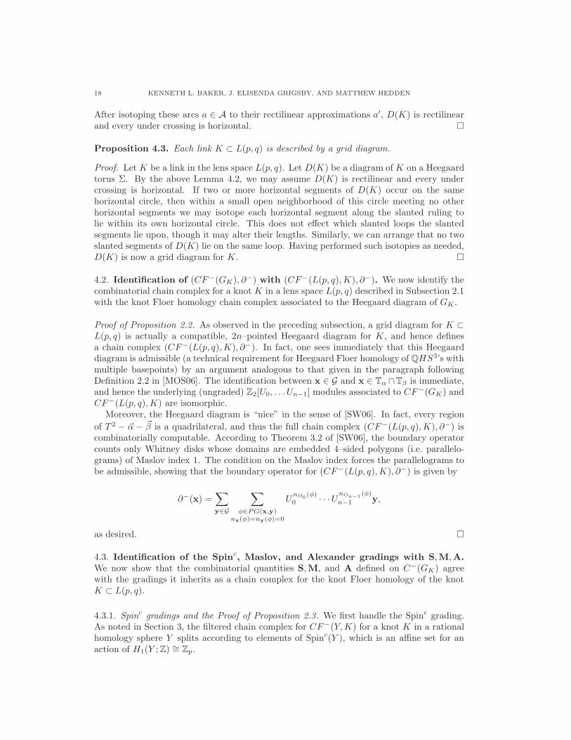
Proposition 4.3. Each link K ⊂ L(p, q) is described by a grid diagram.

Proof. Let K be a link in the lens space L(p, q). Let D(K) be a diagram of K on a Heegaardtorus Σ. By the above Lemma 4.2, we may assume D(K) is rectilinear and every undercrossing is horizontal. If two or more horizontal segments of D(K) occur on the samehorizontal circle, then within a small open neighborhood of this circle meeting no otherhorizontal segments we may isotope each horizontal segment along the slanted ruling tolie within its own horizontal circle. This does not effect which slanted loops the slantedsegments lie upon, though it may alter their lengths. Similarly, we can arrange that no twoslanted segments of D(K) lie on the same loop. Having performed such isotopies as needed,D(K) is now a grid diagram for K.

4.2. Identification of (CF−(GK), ∂−) with (CF−(L(p, q),K), ∂−). We now identify thecombinatorial chain complex for a knot K in a lens space L(p, q) described in Subsection 2.1with the knot Floer homology chain complex associated to the Heegaard diagram of GK .

Proof of Proposition 2.2. As observed in the preceding subsection, a grid diagram for K ⊂L(p, q) is actually a compatible, 2n–pointed Heegaard diagram for K, and hence definesa chain complex (CF−(L(p, q),K), ∂−). In fact, one sees immediately that this Heegaarddiagram is admissible (a technical requirement for Heegaard Floer homology of QHS3’s withmultiple basepoints) by an argument analogous to that given in the paragraph followingDefinition 2.2 in [MOS06]. The identification between x ∈ G and x ∈ Tα ∩Tβ is immediate,and hence the underlying (ungraded) Z2[U0, . . . Un−1] modules associated to CF−(GK) andCF−(L(p, q),K) are isomorphic.

Moreover, the Heegaard diagram is “nice” in the sense of [SW06]. In fact, every region

of T 2 − ~α − ~β is a quadrilateral, and thus the full chain complex (CF−(L(p, q),K), ∂−) iscombinatorially computable. According to Theorem 3.2 of [SW06], the boundary operatorcounts only Whitney disks whose domains are embedded 4–sided polygons (i.e. parallelo-grams) of Maslov index 1. The condition on the Maslov index forces the parallelograms tobe admissible, showing that the boundary operator for (CF−(L(p, q),K), ∂−) is given by

∂−(x) =∑

y∈G

∑

φ∈PG(x,y)nx(φ)=ny(φ)=0

UnO0

(φ)0 · · ·U

nOn−1(φ)

n−1 y,

as desired.

4.3. Identification of the Spinc, Maslov, and Alexander gradings with S,M,A.

We now show that the combinatorial quantities S,M, and A defined on C−(GK) agreewith the gradings it inherits as a chain complex for the knot Floer homology of the knotK ⊂ L(p, q).

4.3.1. Spinc gradings and the Proof of Proposition 2.3. We first handle the Spinc grading.As noted in Section 3, the filtered chain complex for CF−(Y,K) for a knot K in a rationalhomology sphere Y splits according to elements of Spinc(Y ), which is an affine set for anaction of H1(Y ;Z) ∼= Zp.

19

In [OS03], Ozsvath and Szabo construct an affine identification6

φ : Spinc(L(p, q);Z) → Zp.

For the standard singly-pointed genus 1 Heegaard diagram for L(p, q), we have

φ(sO(xO)) = q − 1,

where sO(xO) is the Spinc structure corresponding to the intersection point located in thelower left-hand corner of the region containing O (there, w).

Recall from Subsection 3.1, the map

sO : Tα ∩ Tβ = G → Spinc(Y ).

Composing sO with φ, and considering the Heegaard diagram associated to a grid diagramGK , we obtain a map:

Sf = φ sO : G → Zp.

We wish to show that Sf(x) = S(x) for all x ∈ G, where S is the combinatorial quantitydefined in Subsection 2.2.1. The first step is to show that they agree for a specific elementxO ∈ G.

Lemma 4.4. Let xO be the generator whose components lie in the lower left hand cornersof the regions in GK containing the O basepoints. Then

Sf(xO) = q − 1.

Proof. Take a fundamental domain for GK such that one of the O basepoints is in the lowerleft-hand corner of the grid.7 If we forget about X, we are left with an n–pointed Heegaarddiagram for L(p, q), where n is the grid number of GK .

Beginning with the β circle to the right of this basepoint, let us now handleslide each ofthe β circles over the one immediately to its right. Do this until the β circles on the diagramconsist of a single curve of slope − p

qand n− 1 null-homotopic circles enclosing all but the

left-most Oi. See Figure 5.Now consider the Heegaard triple diagram pictured in Figure 6 with Tα specified by the

original α curves, Tβ specified by the original β curves, and Tγ specified by the β curvesafter we have performed the above sequence of handleslides.

Let y be the generator pictured in Figure 6 in Tα ∩ Tγ by black circles. We claim that

Sf(y) = Sf(xO).

This follows from the existence of a Whitney triangle, ψ connecting xO, y, and a canonicalgenerator Ω ∈ Tβ ∩ Tγ . Indeed, the four-dimensional cobordism, W , corresponding to the

triple of curves (~α, ~β,~γ) is easily seen to be L(p, q) × [0, 1] minus a regular neighborhoodof the solid torus Vβ × 1

2 (see Example 8.1 of [OS04c]). It follows that the restriction ofthe Spinc structure associated to ψ to the L(p, q) boundary components of W must agree.These restrictions, in turn, are sO(y) and sO(xO), respectively, proving the claim.

On the other hand, Sf(y) = q − 1, according to the labeling convention specified inSection 4.1 of [OS03]. Indeed, y is the same generator pictured in Figure 7, for which thislast observation is obvious.

6Both sets admit an action by H1(L(p, q);Z) which, in the case of Zp, comes from an implicit isomorphismH1(Y ;Z) ∼= Zp induced from the Heegaard diagram. Note that while this identification at first sight appearsto be solely in terms of a specific Heegaard diagram for L(p, q), it has a geometric interpretation in termsof the Chern classes of Spinc structures over four-dimensional two-handle cobordisms between lens spaces.

7This choice has no effect on the computation of the absolute Maslov grading, as we will see; it is madeonly so that we can easily describe the procedure.


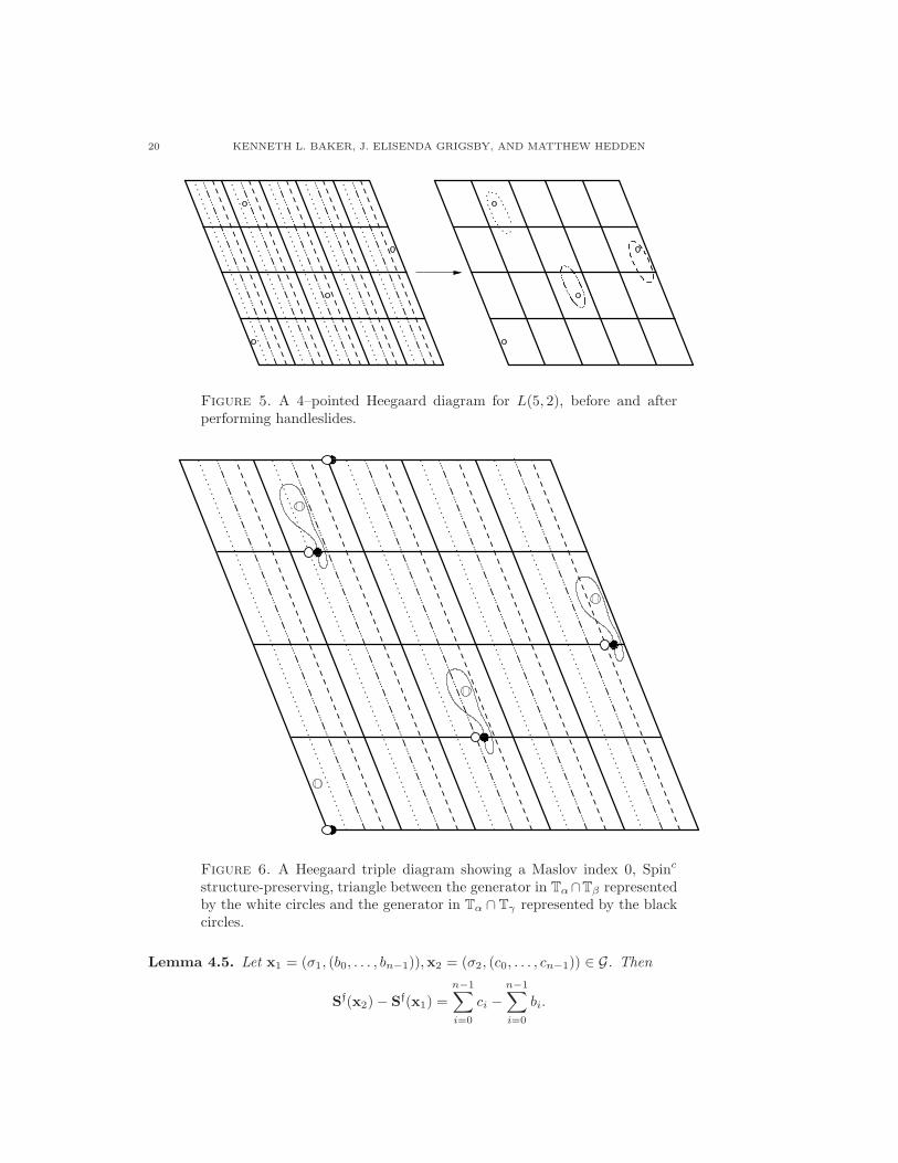
Figure 5. A 4–pointed Heegaard diagram for L(5, 2), before and afterperforming handleslides.

Figure 6. A Heegaard triple diagram showing a Maslov index 0, Spinc

structure-preserving, triangle between the generator in Tα∩Tβ representedby the white circles and the generator in Tα ∩ Tγ represented by the blackcircles.

Lemma 4.5. Let x1 = (σ1, (b0, . . . , bn−1)),x2 = (σ2, (c0, . . . , cn−1)) ∈ G. Then

Sf(x2)− Sf(x1) =n−1∑

i=0

ci −n−1∑

i=0

bi.

21

Figure 7. A generator in a 3–times stabilized Heegaard diagram forL(5, 2). It is the lowest Maslov index generator in CF−(L(p, q); sq−1) (usingnotation from [OS03]), hence has absolute Maslov grading d(L(p, q), sq−1)−(n− 1).

Proof. Lemma 2.19 of [OS04c] indicates that

Sf(x2)− Sf(x1) = sO(x2)− sO(x1) ∈ H1(L(p, q)) ∼= Zp

is represented by any cycle ǫ(x2,x1) obtained by connecting x2 to x1 along the α curvesand x1 to x2 along the β curves. This number, in turn, is the mod p intersection of (a smalltransverse push off of) ǫ(x2,x1) with any of the β curves, say β0.

Furthermore, transverse intersections with β0 of a small horizontal push-off of ǫ(x2,x1)occur only along the horizontal (i.e. α) pieces of ǫ(x2,x1). Along a single α curve, the givenlabeling was chosen to count the number of intersections (mod p) of an arc of the α curvewith β0.

Therefore, the total number of intersections of ǫ(x2,x1) with β0 is

n−1∑

i=0

ci −n−1∑

i=0

bi,

as desired.

Proof of Proposition 2.3. It remains to show that S(x) = Sf(x) for each generator x.With the definition of S preceding Proposition 2.3 observe that, given any

x1 = (σ1, (b0, . . . , bn−1)),x2 = (σ2, (c0, . . . , cn−1)) ∈ G,

Lemma 4.5 implies that S agrees with Sf up to an overall shift:

S(x2)− S(x1) =n−1∑

i=0

ci −n−1∑

i=0

bi = Sf(x2)− Sf(x1).

Lemma 4.4 however shows that S agrees with Sf on the generator xO:

S(xO) = q − 1 = Sf(xO).


Hence the two gradings agree for every generator.

4.3.2. Maslov gradings and the proof of Proposition 2.5.

Proof of Proposition 2.5. We now wish to show that the combinatorial quantity M agreeswith the grading on knot Floer homology, Mf, defined in Subsection 3.1. Our strategy will

be to construct a Heegaard diagram compatible with the lift, K, of K in the universal coverof L(p, q). One easily constructs such a Heegaard diagram which, in fact, is a grid diagram

for K in S3 in the traditional sense [MOS06]. A simple formula for the Maslov grading[MOST06] in the cover, coupled with the relative Maslov index formula of [LL06] and acalculation of the absolute Maslov grading for a single generator completes the proof.

Lemma 4.6. [GRS07] Let T be a twisted toroidal grid diagram for K in L(p, q). Form theuniversal cover R2 of T , identifying T with the fundamental domain

[0, 1]× [0, 1] ⊂ R2

of the covering space action. Let Z be the lattice generated by the vectors (1, 0) and (0, p).Then

T = R2/Z

is a Heegaard diagram compatible with K ⊂ S3, where K is the preimage of K under thecovering space projection π : S3 → L(p, q).

Figure 8 illustrates a grid diagram for K in S3 obtained from a grid diagram of K in

L(p, q). Note that when K is a knot, K will be a link of ℓ = pkcomponents, where k is the

order of [K] as an element in H1(L(p, q);Z).

The chain complex CF−(S3, K) is generated by the points in Teα ∩ Teβ, where α and β

are the lifts in the Heegaard diagram for (S3, K) of the α and β curves for (L(p, q),K).To calculate the relative Maslov gradings between generators x,y ∈ Tα ∩ Tβ , we use thenatural map

Tα ∩ Tβ → Teα ∩ Teβ

which sends a generator x ∈ Tα ∩ Tβ to x = (x, . . . ,x) ∈ Teα ∩ Teβ, the collection of its

preimages, also depicted in Figure 8.

By [LL06], the Maslov grading differences between x,y ∈ G and x, y ∈ G satisfy therelationship:

(1) Mf(x)−Mf(y) =1

p

(Mf(x)−Mf(y)

).

Furthermore, in [MOST06], the authors provide a simple formula for the Maslov indexof a generator in a toroidal grid diagram GK for a pair (S3,K) of a link K in S3. Inparticular, given a point a in a fundamental domain representing GK , let πx(a) denote itsx (horizontal) coordinate and πy(a) denote its y (vertical) coordinate. They then definea function I( · , · ) whose input is two collections, A = (a1, . . . , ar) and B = (b1, . . . , bs) offinitely many coordinate pairs in GK ⊂ R2, the chosen fundamental domain representing theHeegaard torus. This function assigns to the pair (A,B) the number of pairs a ∈ A, b ∈ Bsatisfying πx(a) < πx(b) and πy(a) < πy(b). They go on to show that for a generatorx ∈ CF−(S3,K),

Mf(x) = I(x,x) − I(x,O) − I(O,x) + I(O,O) + 1.

23

S3 S3

=

L(3, 1)ex :x :

Figure 8. A grid number 2 diagram of a knot K with a chain complex

generator x in L(3, 1) and their lifts K and x to a grid number 6 diagramin the universal cover S3.

In particular, Mf is independent of the chosen fundamental domain representing GK .8 Asin [MOST06], we will find it convenient to use a bilinear extension of a symmetrized versionof the I function:

J (A,B) :=1

2(I(A,B) + I(B,A)).

This allows the Maslov grading of a generator in an S3 grid diagram to be expressedmore succinctly as:

Mf(x) = J (x−O,x−O) + 1.

Lemma 4.7. Let GK be a grid number n grid diagram for K ⊂ L(p, q), and let xO denotethe generator corresponding to the lower left corner of the O basepoints. Then

Mf(xO) = d(p, q, q − 1)− (n− 1).

Here d(p, q, q− 1) denotes the correction term d(−L(p, q), q− 1) as defined inductively in[OS03]. See Remark 2.4.

Proof. As in [MOS06], we compute the absolute Maslov grading of the given generator byconnecting it, via a Maslov index 0 triangle in a Heegaard triple diagram, to a generatorwhose absolute Maslov grading we know. See Section 8 of [OS04c] for the definition of a

8We emphasize that the given formula requires a linear identification of GK with a fundamental domainon R2 with the property that α circles correspond to slope 0 lines and β circles to slope ∞ lines. This isequivalent to what we have done: i.e., chosen coordinates on the fundamental domain

(x, y) ∈ R2 | 0 ≤ y < p,−q

py ≤ x < −

q

py + 1

ff

with respect to the basis ~v1 =“

1

np, 0

”

, ~v2 =“

− qnp

, 1

n

”

.


Heegaard triple diagram and Section 7 of [OS06b] for details on computing absolute Maslovgradings.

To do this, we use the same procedure as in the proof of Lemma 4.4, noting that alltriangles involved have Maslov index 0. See Figures 5, 6, 7. It follows that the generatorpictured in Figure 6 in Tα∩Tγ by black circles has the same absolute Maslov grading as thegenerator pictured in Figure 7. This latter generator, in turn, has absolute Maslov gradingd(p, q, q − 1) − (n − 1), since it is the lowest generator in the Spinc structure with Spinc

grading q − 1 for an n − 1 times stabilized Heegaard diagram. See also the discussion inSection 2 of [MOS06].

Lemma 4.8. Let GK be a grid number n grid diagram for K ⊂ L(p, q) and G eKthe asso-

ciated grid diagram for K ⊂ S3. Then

Mf(xO) = −(pn− 1).

Proof. xO is xeO, the generator in the lower-left hand corner of O. Thus one easily checks,

by a calculation analogous to that detailed in the proof of Lemma 6.3 of [OST06], thatMf(xO) = −(N − 1), where N is the grid number (see also Lemma 3.2 in [MOS06]). In thiscase, N = pn.

Thus, we arrive at Equation 2:

Corollary 4.9. Let x ∈ G be a generator associated to GK and x ∈ G its lift in G eK. Then

(2) Mf(x) =1

pMf(x) +

(d(p, q, q − 1) +

p− 1

p

).

Proof. One easily checks using Lemmas 4.7 and 4.8 that this formula holds for xO. Theconclusion then follows from Equation 1.

It is straightforward to verify that the function W , defined in the discussion leading upto the statement of Proposition 2.5, sends a point in GK to the p–tuple of its preimagesin G eK

. Then from Corollary 4.9 it follows that M(x) = Mf(x) for all x ∈ G, proving

Proposition 2.5. Note that since Mf = M is a homological grading on CF−(L(p, q),K), itfollows that M(∂x) = M(x)− 1.

4.3.3. Alexander gradings and the proof of Proposition 2.6. We conclude by identifying A,as defined in Section 2.2.3, with the rational Alexander grading Af.

Proof of Proposition 2.6. By Proposition 2.5, we have M = Mf. Therefore, it will be suffi-cient to show that the definition of the Alexander gradingAf given in Subsection 3.1 satisfiesthe stated relationship. That is, we must show

Lemma 4.10. Let x ∈ Tα ∩ Tβ . Then

(3) AfO,X(x) =

1

2(MO(x)−MX(x)− (n− 1))

A proof of the lemma implies, in particular, that the combinatorial definition of A definesa filtration on (CF−(L(p, q)), ∂−), since this is known to be true for the rational Alexandergrading Af.

Proof of Lemma 4.10. The articles [MOS06] and [MOST06] give combinatorial descriptionsof the Maslov and Alexander gradings for knots and links in S3 and prove these combinatorialdefinitions match the original definitions. Thus our strategy is to pass to the universal cover

of L(p, q) and build a grid diagram for the lift K ⊂ S3 of K corresponding to GK . We then

25

use the behavior of Mf and Af under covers to prove that the stated relationship holds forgenerators in the 2n–pointed Heegaard diagram for L(p, q).

If [K] ∈ H1(L(p, q);Z) has order k, then K will be a link of ℓ = pkcomponents. There is

a natural map

Tα ∩ Tβ → Teα ∩ Teβ

which lifts every generator to the k–tuple of its preimages (cf. the discussion following

Lemma 4.6). Let G denote the set of generators Tα ∩Tβ and similarly let G = Teα ∩Teβ. For

x ∈ G, denote its lift by x ∈ G. Similarly, let MfeO, Mf

eX, and Af

eO,eXdenote the Maslov and

Alexander gradings relative to the lifted basepoints.

We now observe that if there exists a constant C ∈ Z independent of x ∈ G, such that

AfeO,eX

(x) =1

2

(Mf

eO(x)−Mf

eX(x)− (pn− 1)

)+ C

for all x ∈ G, then there exists a(nother) constant C ∈ Q, independent of x ∈ G, such that

AfO,X(x) =

1

2

(Mf

O(x)−MfX(x) − (n− 1)

)+ C,

and hence by Proposition 2.5,

AfO,X(x) =

1

2(MO(x)−MX(x) − (n− 1)) + C.

The observation follows immediately from the fact that the relative Af and Mf gradingstransform in the same way under the covering operation. More precisely, [LL06] tells usthat for any two generators x,y ∈ G, we have:

MfO(x)−Mf

O(y) =1

p(Mf

eO(x)−Mf

eO(y))

and

MfX(x) −Mf

X(y) =1

p(Mf

eX(x)−Mf

eX(y)).

Similarly, Lemma 4.2 in [Ni06a] says that:

AfO,X(x)−Af

O,X(y) =1

p(Af

eO,eX(x)−Af

eO,eX(y)).

Thus

C = AfO,X(x) −

1

2

(Mf

O(x)−MfX(x) − (n− 1)

)

is independent of x ∈ G.To prove the existence of the C discussed above, we will appeal to Equation 2 from

[MOST06]:

Afi(x) = J (x−

1

2(X+ O) , Xi − Oi)−

(ni − 1

2

).

See Subsection 3.1 for the definition of the components, Afi, of the Alexander multi-grading.

Here, the notation Oi (resp. Xi) refers to the subset of O (resp. X) corresponding to theith component of the link, and J is the bilinear extension of a symmetrized version of Iwhich was defined in the discussion immediately preceding the statement of Lemma 4.7.


Now suppose K has ℓ components. We have:

AfeO,eX

(x) =

ℓ∑

i=1

Afi(x)

= J (x−1

2(X+ O) ,

ℓ∑

i=1

(Xi − Oi))−

(pn− ℓ

2

)

= J (x−1

2(X+ O) , X− O)−

(pn− ℓ

2

)

= J (x, X− O)−1

2[J (X, X)− J (O, O)]−

(pn− ℓ

2

)

where equality holds from line 2 to line 3 because J (A,B + C) = J (A,B ∪ C) wheneverB ∩C = ∅.

We now want to verify that this differs by a constant (independent of x) from:

1

2(MeO

(x)−MeX(x)− (pn− 1)) =

1

2(J (x− O, x− O)− J (x− X, x− X)− (pn− 1))

=1

2[−2J (x, O) + J (O, O) + 2J (x, X)− J (X, X)− (pn− 1)]

= J (x, X− O)−1

2[J (X, X)− J (O, O)]−

(pn− 1

2

)

It is now clear that

AfeO,eX

(x) =1

2(MeO

(x)−MeX(x)− (pn− 1)) + C

where C = ℓ−12 , which does not depend on x.

It follows that Equation 3 holds up to an overall shift by a constant, C. But, by Lemma 3.3we know that

AfO,X(x) = −Af

X,O(x)− (n− 1),

which forces C = 0.

References

[Ber] J. Berge, Some knots with surgeries yielding lens spaces. unpublished manuscript.[Ghi06] P. Ghiggini, Knot Floer homology detects genus-one fibered knots. to appear Amer. J. Math.[GJ07] J. Greene and S. Jabuka, The slice-ribbon conjecture for 3-stranded pretzel knots. arXiv:0706.3398v2

[math.GT], 2007.[GRS07] J. E. Grigsby, D. Ruberman, and S. Strle, Knot concordance and Heegaard Floer homology invari-

ants in branched covers. arXiv:math/0701460v2 [math.GT], 2007.[He07] M. Hedden, On Floer homology and the Berge conjecture on knots admitting lens space surgeries.

arXiv:0710.0357v2 [math.GT], 2007.[JN06] S .Jabuka and S. Naik, Order in the concordance group and Heegaard Floer homology.

arXiv:math/0611023v1 [math.GT], 2006.[LL06] D. A. Lee and R. Lipshitz, Covering spaces and Q gradings on Heegaard Floer homology.

arXiv:math/0608001v1 [math.GT], 2006.

[Lip06] R. Lipshitz, A cylindrical reformulation of Heegaard Floer homology. Geom. Topol., 10:955-1097,2006.

[MO05] C. Manolescu and B. Owens, A concordance invariant from the Floer homology of double branchedcovers. arXiv:math/0508065v1 [math.GT], 2005.

http://arxiv.org/abs/0706.3398

http://arxiv.org/abs/math/0701460





27

[MOS06] C. Manolescu, P. Ozsvath, and S. Sarkar, A combinatorial description of knot Floer homology.arXiv:math/0607691v2 [math.GT], 2006.

[MOST06] C. Manolescu, P. Ozsvath, Z. Szabo, and D. Thurston, On combinatorial link Floer homology.arXiv:math/0610559v2 [math.GT], 2006.

[Ni06a] Y. Ni, Link Floer homology detects the Thurston norm. arXiv:math/0604360v1 [math.GT], 2006.[Ni06b] , Knot Floer homology detects fibered knots. to appear Invent. Math.[OS03] P. Ozsvath and Z. Szabo, Absolutely graded Floer homologies and intersection forms for four-

manifolds with boundary. Adv. Math., 173(2):179–261, 2003.[OS04a] , Holomorphic disks and genus bounds. Geom. Topol., 8:311–334 (electronic), 2004.[OS04b] , Holomorphic disks and knot invariants. Adv. Math., 186(1):58–116, 2004.[OS04c] , Holomorphic disks and topological invariants for closed three-manifolds. Ann. of Math.

(2), 159(3):1027–1158, 2004.[OS05a] , Knot Floer homology and rational surgeries. arXiv:math/0504404v1 [math.GT], 2005.[OS05b] , Holomorphic disks and link invariants. arXiv:math/0512286v2 [math.GT], 2005.[OS06a] , Link Floer homology and the Thurston norm. arXiv:math/0601618v3 [math.GT], 2006.[OS06b] , Holomorphic triangles and invariants for smooth four-manifolds. Adv. Math., 202(2):326–

400, 2006.[OST06] P. Ozsvath, Z. Szabo, and D. Thurston, Legendrian knots, transverse knots and combinatorial

Floer homology. math.GT/0611841 [math.GT], 2006.

[Ras03] J. Rasmussen, Floer homology and knot complements. PhD thesis, Harvard University, 2003.[Ras07] , Lens space surgeries and L-space homology spheres. arXiv:0710.2531v1 [math.GT], 2007.[SW06] S. Sarkar and J. Wang, An algorithm for computing some Heegaard Floer homologies.

arXiv:math/0607777v3 [math.GT], 2006.[Tur97] V. Turaev, Torsion invariants of Spinc-structures on 3-manifolds. Math. Res. Lett., 4(5):679–695,

1997.[Tur02] , Torsions of 3-dimensional manifolds, volume 208 of Progress in Mathematics. Birkhauser

Verlag, Basel, 2002.

Kenneth L. Baker

School of Mathematics

Georgia Institute of Technology

Atlanta, Georgia 30332

E-mail address: [email protected]

J. Elisenda Grigsby

Department of Mathematics

Columbia University

2990 Broadway MC4406

NY, NY 10027


Matthew Hedden

Department of Mathematics

Massachusetts Institute of Technology

Building 2, Room 236

77 Massachusetts Avenue

Cambridge, MA 02139-4307











floer homology kenneth l. baker, j. elisenda grigsby, …

Documents