NOTICE: this is the authors version of a work that was accepted for publicationin Combustion and Flame. Changes resulting from the publishing process, suchas peer review, editing, corrections, structural formatting, and other qualitycontrol mechanisms may not be reflected in this document. Changes may havebeen made to this work since it was submitted for publication. A definitiveversion was subsequently published in Combustion and Flame,https://doi.org/10.1016/j.combustflame.2017.02.012

Flame resolved simulation of a turbulent premixedbluff-body burner experiment.

Part II: A-priori and a-posteriori investigation ofsub-grid scale wrinkling closures in the context of

artificially thickened flame modeling

Fabian Procha,∗, Pascale Domingob, Luc Vervischb, Andreas M. Kempfa

aChair of Fluid Dynamics, Institute for Combustion and Gasdynamics (IVG), University ofDuisburg-Essen, 47048 Duisburg, Germany

bCORIA - CNRS, Normandie Universite, INSA de Rouen, Technopole du Madrillet, BP 8,76801 Saint-Etienne-du-Rouvray, France

Abstract

Dynamic sub-filter closures for artificially thickened flame (ATF) combustion

models for large eddy simulation (LES) are investigated with consistent a-priori

and a-posteriori analyses. The analyses are based on a flame resolved simulation

(quasi DNS) and large eddy simulations of the bluff body burner experiment

by Hochgreb and Barlow with premixed flamelet generated manifolds (PFGM).

Both flame resolved simulation and LES are performed under the conditions of

a single real flame experiment, using the same domain size, filter sizes, bound-

ary conditions and numerics, all with an additional validation by comparison to

experimental data. For the evaluation of the sub-filter wrinkling factor, the well-

established model by Charlette et al. (2002) in the modified version by Wang

et al. (2011) is used with a static and with a dynamic model parameter, a new

dynamic power-law model is discussed additionally. In the a-priori analysis,

the probability density functions (PDFs) of the sub-grid scale (SGS) wrinkling

factor are compared against the modeled ones based on the flame resolved sim-

ulation data. These a-priori modeled wrinkling factor PDFs are then compared

∗Corresponding authorEmail address: fabian.proch@uni-due.de (Fabian Proch)

Preprint submitted to Combustion and Flame February 6, 2017

against the a-posteriori ones from the LES results, where a similar shape is

observed for all models. The static model tends to over-predict the wrinkling

factor, a better agreement is found for the dynamic models for the medium

and small filter width, where the new formulation improves the results for the

latter. For the largest filter width, the wrinkling factor is under-predicted by

the dynamic models. This under-prediction is, however, compensated by larger

gradients of the progress variable field so that the mean flame surface density

conditioned on the progress variable is in closer agreement with the flame re-

solved simulation than the wrinkling factor PDFs are. Finally, radial profiles

of the time-averaged temperature from the LES, flame resolved simulation and

experiment are compared against each other. With the dynamic SGS wrinkling

models, the LES results converge with grid refinement against the flame resolved

simulation results.

Keywords: Turbulent premixed combustion, SGS wrinkling model, Dynamicmodeling, Direct numerical simulation, Large eddy simulation

1. Introduction

Premixed flames are too thin to be resolved on cell sizes that are affordable in

Reynolds-averaged Navier-Stokes (RANS) simulations or large eddy simulations

(LES) of technical combustors. One possible alternative is to artificially thicken

the flame (ATF) [1–5]. Although the ATF (or thickened flame LES, TFLES)

approach preserves the self-induced propagation speed of the local interface

between fresh and burnt gases, the response of the thickened reaction zone to

turbulence differs from the original one. Therefore, additional modeling of the

sub-grid scale wrinkling is required.

Among the models for sub-filter flame wrinkling, the one developed by Charlette

et al. [4] has been frequently used with ATF with good success. This closure

involves an exponent β that is related to the fractal dimension D of the flame

surface by β = D− 2 and may either be set to a fixed value (typically β = 0.5),

or alternatively be determined from a dynamic procedure. The performance

2

and validity of the dynamic procedure has been assessed before a-priori based

on DNS results [6–9] and a-posteriori based on LES results [6, 8–12]. In these

investigations, the dynamic procedure was applied in a formulation averaged for

small volumes, over a homogeneous direction, or over the whole domain. The

resulting β value was found to vary in space and time, generally β grew with

the distance from the burner exit and with decreasing mesh resolution.

In most studies of SGS wrinkling modeling, DNS and LES were not per-

formed under the same flow conditions (for obvious resolution requirements),

making it hard to draw definitive conclusions, for example about the role of

compensating errors. The present work aims to further investigate the dynamic

sub-filter modeling for thickened and filtered flame combustion models, with a

consistent a-priori (flame resolved simulation, quasi a DNS) and a-posteriori

(LES) analysis. Flame resolved simulation and LES are performed under the

conditions of a single real flame experiment, using the same domain size, filter

sizes, boundary conditions and numerics, all with an additional validation by

comparison to experimental data [13–18]. The first model that is investigated

is the one by Charlette et al. [4] in the modified version by Wang et al. [10] with

either a constant, or a dynamic model parameter [6, 9]. A new dynamic power-

law model is then presented, where the lower cutoff depends on the sub-filter

turbulence intensity and on the laminar flame speed.

The investigations are carried out for a premixed bluff body burner [13], for

which a database from a flame resolved simulation is available [19]. In this flame

resolved simulation, the progress variable and velocity fields were fully resolved

inside the relevant flame region in a DNS-sense, although a small amount of

unresolved velocity fluctuations is still present in the unburnt gas, away from

the reaction zones. This database is used for the a-priori analysis, LES of the

same burner are also reported to further assess the modeling.

3

2. Modeling approach

2.1. Combustion model

The focus of this work is on the investigation of sub-filter modeling for a

real methane-air flame experiment over a wide range of filter widths, detailed

chemistry tabulation was chosen to make the study computationally afford-

able: The premixed flamelet generated manifolds (PFGM) approach [20] has

demonstrated its efficiency and suitability in previous work [e.g. 21–26] already.

Transport equations were solved in the flame resolved simulation and LES for

the (non-normalized) progress variable YC = YCO2+ YCO + YH2O based on

product mass fractions and for the mixture fraction Z. The mixture fraction is

linked to the fresh gas equivalence ratio by φ = [Z (1− Zs)]/

[Zs (1− Z)] with

the stoichiometric methane-air mixture fraction Zs = 0.054.

Freely-propagating methane-air flames for varying initial compositions were

computed with ‘Cantera’ [27] using the GRI-3.0 mechanism [28]. A Lewis num-

ber of unity was assumed for all species, which has only a negligible influence

on the propagation speed of the flame for the lean equivalence ratios present in

the studied burner [29].

The results were stored in a two-dimensional equidistant lookup table as a

function of the mixture fraction Z and the normalized progress variable C =

YC/YbC(Z), where the superscript b denotes the fully burnt state. Below the

lean flammability limit of φ = 0.45, a linear interpolation was used for the

species mass fraction and the enthalpy. More details on the chemistry model

are available from previous papers [19, 21, 22].

2.2. ATF model

To make the premixed flame resolvable on the LES grid, the artificial thick-

ened flame (ATF) model [1, 3, 4] was applied. The broadening of the reaction

zone is achieved by increasing the diffusivity by a thickening factor FD and by

decreasing the source term by the same factor in the Favre-filtered transport

4

equation for the progress variable [29, 30]:

∂ρYC∂t

+∇ ·(ρ~uYC

)=

∇ ·([FD Ξ∆

λ

cp+ (1− Ω)

µtSct

]∇YC

)+

Ξ∆

FDωC

(1)

Favre-filtering of a quantity φ is denoted by φ and Reynolds-filtering by φ ,

the Favre-filtered velocity vector is represented by ~u. The fluid density ρ, the

thermal conductivity λ, the heat capacity cp and the progress variable source

term ωC are obtained from the PFGM table. Outside of the reaction zone,

the effect of the unresolved velocity scales is modeled by an eddy diffusivity

approach, which is blended in gradually with the flame sensor Ω [21, 25, 26]. We

studied the effect of this additional (turbulent diffusivity) term on the turbulent

flame propagation and found it to be very small. The turbulent viscosity µt is

computed according to the σ-model by Nicoud et al. [31], with a modeling

constant of Cσ = 1.5 and the turbulent Schmidt number set to Sct = 0.7. The

σ-model is retained even for the flame resolved simulation, but the turbulent

viscosity is less than 10% of the laminar viscosity throughout the flame [19] in

this case. In this context, the interaction between the filtered flame propagation

and the modeling of the sub-filter scalar fluxes has been investigated in detail

by Klein et al. [32, 33].

The thickening factor FD is computed as a function of the normalized progress

variable to avoid unnecessary thickening of the preheat- and burnout zones [30]:

FD(C∗, Z) =(dC/dx)|C=C∗

(dC/dx)|C=C∗

(2)

The numerator (dC/dx)|C=C∗ represents the gradient of the C-profile, taken

at C = C∗, resulting from the computation of a one-dimensional freely prop-

agating and unstrained premixed flame for the respective mixture fraction Z.

The denominator (dC/dx)|C=C∗ is obtained from Gaussian-filtering, at the fil-

ter width ∆, of the same C-profile and computing the resulting gradient at

C = C∗. Using the dynamic thickening factor formulation given by Eq. 2 in the

ATF model exactly reproduces the Gaussian-filtered profile for a one dimen-

5

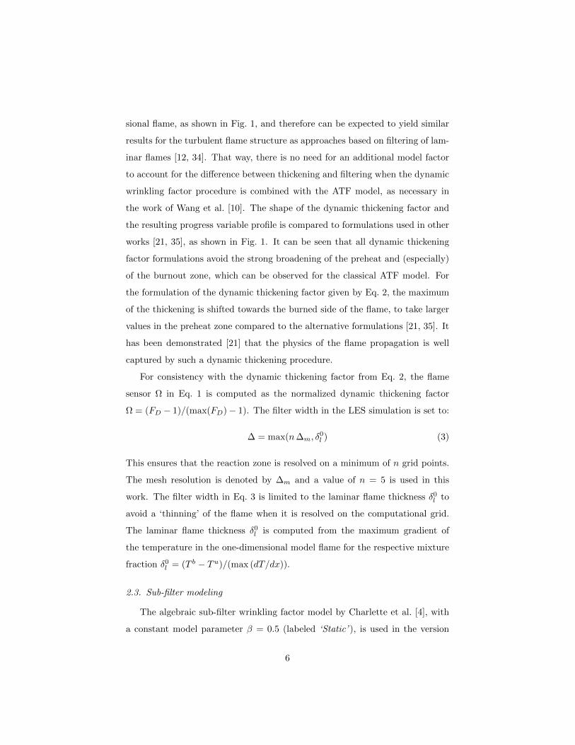
sional flame, as shown in Fig. 1, and therefore can be expected to yield similar

results for the turbulent flame structure as approaches based on filtering of lam-

inar flames [12, 34]. That way, there is no need for an additional model factor

to account for the difference between thickening and filtering when the dynamic

wrinkling factor procedure is combined with the ATF model, as necessary in

the work of Wang et al. [10]. The shape of the dynamic thickening factor and

the resulting progress variable profile is compared to formulations used in other

works [21, 35], as shown in Fig. 1. It can be seen that all dynamic thickening

factor formulations avoid the strong broadening of the preheat and (especially)

of the burnout zone, which can be observed for the classical ATF model. For

the formulation of the dynamic thickening factor given by Eq. 2, the maximum

of the thickening is shifted towards the burned side of the flame, to take larger

values in the preheat zone compared to the alternative formulations [21, 35]. It

has been demonstrated [21] that the physics of the flame propagation is well

captured by such a dynamic thickening procedure.

For consistency with the dynamic thickening factor from Eq. 2, the flame

sensor Ω in Eq. 1 is computed as the normalized dynamic thickening factor

Ω = (FD − 1)/(max(FD)− 1). The filter width in the LES simulation is set to:

∆ = max(n∆m, δ0l ) (3)

This ensures that the reaction zone is resolved on a minimum of n grid points.

The mesh resolution is denoted by ∆m and a value of n = 5 is used in this

work. The filter width in Eq. 3 is limited to the laminar flame thickness δ0l to

avoid a ‘thinning’ of the flame when it is resolved on the computational grid.

The laminar flame thickness δ0l is computed from the maximum gradient of

the temperature in the one-dimensional model flame for the respective mixture

fraction δ0l = (T b − Tu)/(max (dT/dx)).

2.3. Sub-filter modeling

The algebraic sub-filter wrinkling factor model by Charlette et al. [4], with

a constant model parameter β = 0.5 (labeled ‘Static’ ), is used in the version

6

Figure 1: Left: Comparison of the dynamic thickening factor as a function of the

progress variable computed from Eq. 2 (Fil) to the formulations of Durand and

Polifke (Dur [35]), Proch and Kempf (Pro [21]) and a constant thickening factor

(Con) for a filter width of ∆ = 5.0 mm and an equivalence ratio of φ = 0.75.

Right: Resulting progress variable profiles compared to the original laminar

flame profile (dashed line). The Gaussian-filtered laminar flame profile is indi-

cated by black circles, it is identical to the profile resulting from the dynamic

thickening factor computed from Eq. 2 (Fil).

modified by Wang et al. [10] and will be denoted as Charlette/Wang model in

the remaining part of the paper:

Ξ∆ =

(1 + min

[F − 1,Γ∆

(F,u′

∆

s0l

, Re∆

)u′

∆

s0l

])β(4)

The Charlette/Wang model was chosen as it is (probably) the most frequently

used sgs model in the ATF context and it is still developing and evolving [7, 9,

10, 12, 21, 25]. Therefore, an extensive investigation of the model by a-priori

and a-posteriori analysis with respect to dynamic model formulations is of high

relevance. The Wang et al. [10] formulation in Eq. 4 differs from the original

formulation by Charlette et al. [4] by the subtraction of unity from the thickening

factor, which gives the correct reduction of the wrinkling factor to unity for a

thickening factor of unity in combination with non-vanishing sub-filter velocity

fluctuations u′

∆. The correct capturing of this limiting behavior was not critical

for the original Charlette model, which was designed under the assumption of

large thickening factors that is no longer valid for the fine grid resolutions used

nowadays [10]. The wrinkling factor predicted by the modified Charlette/Wang

7

model is always lower or equal compared to the wrinkling factor predicted by

the original Charlette model. The maximum thickening factor entering the

Charlette/Wang model (Eq. 4) is computed from:

F =∆

δ0l

(5)

It must be stressed that the maximum thickening factor F is basically just an

abbreviation for the ratio of the upper cutoff (the filter width) and the lower

cutoff (the laminar flame thickness) entering the fractal Charlette/Wang model

and therefore has a different role than the dynamic thickening factor FD entering

Eq. 1, although the maximum value of FD is usually equal to F . The laminar

flame speed is denoted by s0l , the sub-filter velocity fluctuations are computed

from the expression given by Colin et al. [3]:

u′

∆ = 2∆3m

∣∣∣∇2(∇× ~u

)∣∣∣ ( n10

) 13

= 2∆3m

∣∣∣∇× (∇2~u)∣∣∣ ( n

10

) 13

(6)

The detailed formulation of the efficiency function Γ∆ that corrects for the

unresolved velocity scales is omitted for brevity, it can be found in previous

publications [3, 4, 10, 21]. It should however be noted that in the majority of

points in the performed LES, the turbulence is so high that Ξ∆ (Eq. 4) saturates

at its maximum value, which is also the case in most practical applications

[9, 12]:

Ξ∆ =

(∆

δ0l

) β

= F β (7)

For the second investigated sub-filter model (labeled ‘DynRef’ ), the param-

eter β is evaluated from a dynamic procedure, which assumes that β is approxi-

mately independent of the filter width. It is also assumed that the same level of

flame surface density is obtained by test-filtering the resolved flame surface den-

sity in the LES, and by computing the flame surface density of the test-filtered

LES progress variable field [9]:⟨Ξ∆ |∇C|

⟩=⟨

Ξγ∆|∇C|⟩

(8)

Here, γ =√

∆2 + ∆2/∆ represents the effective filter width ratio when com-

bining the LES filter ∆ and the Gaussian test filter ∆, where the filter kernel is

8

given as:

G(x, y, z) =

(6

π ∆2

)3/2

exp

[− 6

∆2(x2 + y2 + z2)

](9)

The test-filter width was set equal to the LES filter width ∆ = ∆ in this work,

leading to a filter width ratio of γ =√

2. The influence of the filter width

ratio on the results was studied and found to be small, therefore a compact

test-filter width was chosen to ensure scale similarity. The operator 〈·〉 denotes

spatial averaging, introduced to avoid unphysical local peaks of the dynamic

wrinkling factor. In contrast to former works [9, 12], the averaging operation is

not replaced by a Gaussian filter. This allows to use a more compact averaging

volume, it was found that an averaging volume of 5x5x5 points centered at the

respective grid point was sufficient in the LES due to the equal weighting of

the averaging points. This more localized formulation of the model potentially

improves the applicability to complex flows and geometries that are found in

practical combustors. We found no notable influence on the results when using

the dynamic version of the full Charlette/Wang model (Eq. 4) in the LES on

the coarse grid and therefore used the simpler and numerically cheaper power-

law formulation (Eq. 7) throughout this work, which is in line with former

works [9, 12]. The final formulation of the model (DynRef ) reads:

Ξ∆ =

⟨∆

δ0l

⟩ β

= 〈F 〉 β with β = ln (Ξr) / ln (γ) (10)

Here, Ξr represents the resolved part of the wrinkling factor:

Ξr =⟨|∇C|

⟩ / ⟨|∇C|

⟩≈⟨|∇C|

⟩ / ⟨|∇ C|⟩ (11)

Veynante and Moureau [9] have recently demonstrated that this model is nearly

equivalent to the dynamic similarity model by Knikker et al. [36]. They dis-

cussed how the first RHS of Eq. 11 can be approximated by the second RHS in

the LES, as the Favre-filtered governing equations are solved [9]. They further-

more addressed that this approximation of the filtered progress variable C by

the Favre-filtered progress variable C would be fully valid only for an infinitely

thin flame front, and how the resulting error is reduced by the additional spa-

tial averaging used in Eq. 11. It must however be stressed that the impact of

9

the filtering type on the wrinkling factor field predicted by the dynamic model

is smaller than the impact of the filtering type on the progress variable field

itself (this may be illustrated for a laminar planar flame, where the wrinkling

factor predicted by the dynamic model is unity, independent of the filtering

type, although the filtered progress variable field is significantly influenced by

the filtering type). In the present work, we quantify the error resulting from

the use of the Favre-filtering by performing the a-priori analysis in Section 4.1

for the filtered as well as for the Favre-filtered progress variable and show that

the effect of the filtering type on the predicted wrinkling factor is actually only

minimal.

The starting point for the third investigated model (labeled ‘DynNew’ ) is

also the fractal power-law formulation given by Eq. 7, which assumes a con-

stant lower cutoff scale equal to the laminar flame thickness δ0l . It has been

discussed extensively in the literature that the lower cutoff actually depends on

the intensity and structure size of the turbulence as well as on the (laminar)

flame thickness and propagation speed, various models for the lower cutoff scale

with different results have been proposed in the past [9, 37–40]. This accounts

for the effect of turbulent fluctuations on the gradient of the flame, which is

likely to become important for higher turbulence intensities and has been re-

ported for the investigated burner [19] and in various previous works [41–44].

We tried multiple formulations for the lower cutoff and found that replacing

the constant lower cutoff by δ0l (s0

l /u′

∆)a improves the model performance in the

a-priori analysis. To avoid wrinkling factors smaller than unity, the maximum

value of the lower cutoff scale is limited to the value of the upper cutoff scale

∆, the final model (DynNew) reads:

Ξ∆ =

∆

min(〈δ0l 〉⟨s0lu′∆

⟩a,∆)β

= max

(⟨u′∆s0l

⟩a〈F 〉

) β

, 1

(12)

If the sub-filter velocity fluctuations are equal to the laminar flame speed, Eq. 12

reduces to Eq. 7. For sub-filter velocity fluctuations lower than the laminar flame

speed, Eq. 12 predicts a decreased wrinkling factor due to the increase of the

10

Figure 2: Comparison of the wrinkling factor resulting from the static and dy-

namic Charlette/Wang models (Static, DynRef) and the new model (DynNew),

as a function of the maximum thickening factor F (Eq. 5, left) and the resolved

wrinkling factor Ξr (Eq. 11, right). The effective filter width ratio was set to

γ =√

2, the ratio of the sub-filter velocity fluctuations to the laminar flame

speed to u′

∆/s0l = 10.

lower cutoff scale similar to the full Eq. 4. In case of the sub-filter velocity

fluctuations being greater than the laminar flame speed, Eq. 12 predicts an

increased wrinkling factor as a consequence of the decreased lower cutoff scale.

The a-priori and the a-posteriori analyses were carried out for different values

of the exponent a to study the sensitivity of the model to it. It was found that

the model is not overly sensitive to the value of a, a value of a = 0.1 yielded

the overall best model performance for all filter-widths a-priori and a-posteriori

and was therefore used for the following investigations. The coefficient β in

Eq. 12 is computed again from the dynamic procedure given by Eq. 8:

β =ln (Ξr)

ln

((γ1/3〈u′∆/s0l 〉)a

(γ 〈F 〉)〈u′∆/s0l 〉a 〈F 〉

) =ln (Ξr)

ln(γ1+a/3

) (13)

Figure 2 shows a comparison of the wrinkling factors resulting from the

new model (DynNew) and from the dynamic (DynRef) and static (Static)

Charlette/Wang model, versus the maximum thickening factor F and the re-

solved wrinkling factor Ξr. The filter width ratio was set to γ =√

2, the ratio

of the sub-filter velocity fluctuations to the laminar flame speed to u′

∆/s0l = 10,

which is a representative value in the downstream region of the burner [19]. The

11

wrinkling factor predicted by all models increases as a function of the thickening

factor, with a slope that decreases towards larger values of F . For a thickening

factor of unity, the static and dynamic version of the Charlette/Wang model

predict a wrinkling factor of unity. Due to the aforementioned dependency of

the lower cutoff scale on the sub-filter velocity fluctuations, the new model pre-

dicts a remaining wrinkling factor of (u′

∆/s0l )a β for a thickening factor of unity

when the turbulent sub-filter velocity fluctuations are larger than the laminar

flame speed. This corresponds to a situation where the local progress variable

gradient is increased by the turbulence induced strain, i.e. where the turbulent

flame brush is thinner than the laminar flame thickness. The wrinkling factor

resulting from the static Charlette/Wang model is independent of the resolved

wrinkling factor, whereas the wrinkling factor resulting from both dynamic mod-

els (DynRef, DynNew) increases as a function of the resolved wrinkling factor,

with a slope that decreases towards larger values of the resolved wrinkling fac-

tor. The new model predicts slightly larger wrinkling factors than the dynamic

Charlette/Wang model, most significantly for larger values of the resolved wrin-

kling factor and smaller values of the thickening factor. For a resolved wrinkling

factor of unity in combination with non-vanishing velocity fluctuations, which

indicates that the wrinkling is fully resolved on the computational grid but tur-

bulent motion and flame surface are not in equilibrium [9], both dynamic models

predict the correct wrinkling factor of unity, whereas the static model predicts

a wrinkling factor greater than unity.

3. Numerical setup for LES and flame resolved simulation

The investigated burner has been build and examined at the University of

Cambridge by Hochgreb and co-workers and was also investigated at the Sandia

National Labs by Barlow et al. [13–18]. It consists of a central bluff-body

that is surrounded by two co-annular premixed streams of methane-air with an

equivalence ratio of φ = 0.75. These streams are surrounded by a co-flow of air,

the burner is operated at 295 K and ambient pressure. The burner is illustrated

12

in Fig. 3. The bulk velocities in the inner stream, the outer stream and the co-

flow are 8.31, 18.7 and 0.4 m/s, respectively. This results in Reynolds number

of approximately 5,960 and 11,500 in the inner and outer stream, respectively.

The burner was investigated with LES by different groups [12, 21, 34, 45, 46]

already and is a target of the TNF workshop [47].

The flame resolved simulation was performed with a grid resolution of 0.1 mm,

which is fine enough to resolve the flame with the PFGM-approach without any

thickening. However, in the fresh gas in the shear layers upstream of the nozzle

exit, this grid resolution is not sufficient to fully resolve the Kolmogorov scale.

It was demonstrated in the previous analysis of the flame resolved simulation

fields [19] that the influence of these scales stays very moderate and gets negli-

gible in the flame region for which the following investigations are performed.

The simulations were conducted with the ‘PsiPhi’ code that solves the Navier-

Stokes equations in a Low-Mach number formulation and was developed by

Kempf and co-workers [19, 21–23, 48, 49]. The investigated configuration is

unbounded and without thermoacoustic interactions with a maximum Mach

number of well below 0.1, therefore the low-Mach number formulation can be

expected to not influence the results while enabling a much larger computa-

tional time step. The code was parallelized using the message passing inter-

face (MPI), where non-blocking communication with overlayed computational

work ensures high parallel efficiency. The convective fluxes for momentum and

scalars were discretized by a central difference and a total variation diminish-

ing (TVD) scheme with the non-linear CHARM limiter [50], respectively. The

TVD scheme ensures the boundedness of the scalar transport while avoiding the

excessive smoothing of upwind-schemes. The Poisson-equation for the pressure

was solved with a successive over-relaxated Gauss-Seidel solver. At the inlet,

pseudo turbulent fluctuations with magnitudes of 10% of the bulk velocities and

an integral length-scale of 0.5 mm were imposed by the filtering method intro-

duced by Klein et al. [51] in its numerically efficient implementation [52]. Zero

gradient boundary conditions were set at the outlet for all transported quanti-

ties. The last 12 mm of the burner geometry were included in the simulation

13

domain with the immersed boundary technique. The computational domain

size was 112×120×120 mm, leading to an overall number of 1.6 billion equidis-

tant Cartesian grid cells for the flame resolved simulation. The simulations were

performed on up to 64,000 Blue Gene/Q cores on the JUQUEEN machine at

the Julich Supercomputing Centre, 0.34 seconds of physical time were simulated

for properly sampled statistics, corresponding to 24 flow-through times of the

inner stream, at a total cost of 10 million core hours.

Figure 3 shows instantaneous contour plots for the axial and radial velocity

component, the temperature and the equivalence ratio in the burner-mid section.

It was found in the previous analysis of the flame resolved simulation data [19]

that the flame develops two characteristic regions, due to the different levels

of turbulence in the inner and outer stream. These regions should be treated

separately for a meaningful analysis of the flame dynamics. Therefore, the

analysis is carried out separately for the ‘near ’ and ‘far ’ region, reaching from

0 to 35 mm and from 35 to 70 mm above the burner, respectively. These two

regions are indicated in Fig. 3 by dashed lines, where the higher level of flame

wrinkling in the far region compared to the near region becomes visible, for

instance when inspecting the temperature plot.

For the a-priori analysis, the progress variable field from the flame resolved

simulation was filtered at the filter-widths ∆ and subsequently test-filtered at

∆ as given in Table 1. To be able to compute the filtering operations with the

required large stencils with up to 503 cells in a feasible amount of computational

time, the Gaussian filter was implemented in a sequential order for the three

spatial directions as described by Kempf et al. [52], exploiting the advantages

of the applied simple grid structure.

For the a-posteriori analysis, LES with the grid resolutions given in Table 1

were performed for all three models. The CFD solver, the numerical setup, the

boundary conditions and the FGM model were the same as for the flame resolved

simulation. The only difference between LES and flame resolved simulation was

the use of the ATF model combined with the respective sub-filter model. The

dynamic procedure applied at every computational point for every time step

14

Figure 3: Contour plots in the burner mid-section for the axial velocity com-

ponent (U), radial velocity component (V), Temperature (T) and equivalence

ratio (Eq) from the flame resolved simulation of the investigated burner [19].

The ‘near’ and ‘far’ region for the subsequent analysis are separated by dashed

lines.

15

Table 1: Parameters of the simulations: LES cell size ∆m, ATF filter width

∆, test-filter width ∆, effective filter width ratio γ, averaging-box width 〈∆〉,

maximum thickening factor F and number of computational cells nCells used

in the a-priori and a-posteriori analyses. The laminar flame thickness for the

thickening factor calculation was set to δL = 0.565 mm corresponding to the

inlet equivalence ratio of φ = 0.75. For the finest grid (F), the filter width for

the a-priori analysis (given in brackets) had to be set to a multiple of the flame

resolved simulation mesh resolution of 0.1 mm and therefore slightly deviates

from the a-posteriori width.

∆m ∆ ∆ γ 〈∆〉 F nCells

mm mm mm mm M

Coarse (C) 1.0 5.0 5.0√

2 5.0 8.8 1.7

Medium (M) 0.5 2.5 2.5√

2 2.5 4.4 13.8

Fine (F) 0.25 1.25 (1.2) 1.25 (1.2)√

2 1.25 (1.2) 2.2 (2.1) 106.0

Flame resolved simulation (RES) 0.1 - - - - - 1612.8

increased the computational costs of the LES by around 30%.

4. Results

4.1. A-priori analysis of the wrinkling factor PDFs

The progress variable field C from the flame resolved simulation and the

absolute value of its gradient |∇C| were filtered at the respective filter width

∆. The reference wrinkling factor value from the flame resolved simulation was

then computed from ΞRES∆ =⟨|∇C|

⟩/⟨|∇C|

⟩. Here, the averaging was done

over the same volume as in the LES, which corresponds to 123, 253 and 503

averaging points for the fine, medium and large filter width, respectively.

The resulting filtered progress variable field C and the absolute value of its

gradient |∇C| were filtered again at the test-filter width ∆. Afterwards, the

investigated models were used to compute the wrinkling factors as a function of

the resolved wrinkling factor Ξr =⟨|∇C|

⟩/⟨|∇C|

⟩, the maximum thickening

16

Figure 4: A-priori PDFs of the modeled wrinkling factors (solid lines) and the

exact wrinkling factor (dashed lines) for the filter widths given in Table 1. The

analysis is carried out separately for the near and far region of the burner (see

Section 3) (x-axis is scaled individually).

factor F and the effective filter width ratio γ together with the mixture fraction

and velocity field from the flame resolved simulation. The sub-filter velocity

fluctuations were computed based on the flame resolved simulation velocity

field with Eq. 6. As mentioned before, the same procedure was repeated for

Favre-filtering by replacing C with C.

Figure 4 shows the probability density functions (PDFs) of the a-priori mod-

eled wrinkling factors compared to the exact wrinkling factors from the flame

resolved simulation, where separate PDFs were computed for the weakly tur-

bulent near burner region and the more turbulent region far from it. All com-

putational points inside the flame region, i.e. 0.01 < C < 0.99, were taken

into account, with the exception of points where the thickening factor, or the

exact wrinkling factor, was smaller than 1.001. This additional constraint was

included to avoid a bias of the PDFs towards unity, which indicates a resolved

17

flame, and affected less than 5% of the points in the flame region. The total

number of points used for the generation of the individual PDFs was more than

5 Million. With growing filter width, the PDFs of the exact wrinkling factor

get broader and the peak values get shifted towards higher wrinkling factor val-

ues, as expected. The PDFs are much broader in the far region than in the

near region, due to the higher level of turbulence in the far region which comes

along with additional flame wrinkling. The static model (Static) shows nearly

bimodal PDFs, where the first peak is located at a wrinkling factor of unity and

the second one at the maximum wrinkling factor value from Eq. 7. The peak at

unity can be explained by an efficiency function Γ∆ value of zero, due to zero

sub-filter velocity fluctuations.

The two dynamic models (DynRef and DynNew) are both able to capture

the principal shape of the wrinkling factor PDF for the smallest and the interme-

diate filter width. However, for the largest filter width notable differences exist

between the PDFs of the modeled and the exact wrinkling factor, in general

the dynamic models under-predict the wrinkling factor. This is mostly visible

in the far region, where the peaks of the modeled wrinkling factor PDFs are lo-

cated at significantly smaller values than the peaks of the exact wrinkling factor

PDFs. A potential explanation of this under-prediction of the wrinkling factor

is that finger-like structures vanish during the first filtering operation. In the

subsequent test-filtering operation, these regions appear as closed and smooth,

thus only very little or no wrinkling is predicted there by the dynamic models.

This behavior is illustrated in Fig. 5, which shows cross sections of the original

progress variable field and of the resulting progress variable fields after the first

and second filtering operation with the largest filter width. Furthermore, Fig. 5

includes the relative deviation of the wrinkling factor resulting from the dynamic

Charlette/Wang model from the exact wrinkling factor in the respective cross

section. Four regions with a large under-prediction of the wrinkling factor are

marked by circles, in all of these regions the originally strongly wrinkled flame

structure is vastly smoothened during the first filtering operation, so that the

effect of the second filtering operation is only minute. A further explanation is

18

Figure 5: Illustration of the underestimation of the wrinkling factor by the

dynamic models for the largest filter width in a cross-section 50 mm downstream

of the burner exit. Shown are the unfiltered progress variable C (top left), the

filtered progress variable (Cf, top right), the subsequently test-filtered progress

variable (Cff, bottom left) and the relative deviation of the wrinkling factor

resulting from the dynamic Charlette/Wang model from the exact wrinkling

factor (RelErrXi, bottom right). The circle diameter corresponds to the filter

width of 5 mm, the location of the circles 1-4 is the same in all plots.

19

Figure 6: A-priori PDFs of the normalized deviation of the modeled (DynNew,

DynRef, Static) from the exact (REF) wrinkling factor. The analysis is carried

out separately for the near and far region of the burner (see Section 3). The

solid lines result from Reynolds-filtering, the dashed lines from Favre-filtering.

that the scale similarity, which is the underlying assumption for the dynamic

models, is no longer sufficiently fulfilled at the largest filter width. The modeled

wrinkling factor PDFs for the largest filter width are indeed relatively similar

to the ones for the intermediate filter width. This suggests that an ‘upper cut-

off’ has been reached, above which additional test-filtering yields not enough

information to reconstruct the flame wrinkling with high accuracy.

To enable a detailed local comparison of the investigated wrinkling factor

models, Fig. 6 shows the PDFs of the normalized deviation of the modeled

wrinkling factors from the exact one (DNS). In general, the PDFs get broader

with an increase of the filter width and growing distance from the burner.

The static Charlette/Wang model gives broad PDFs of the deviation with

heavy tails on the right, meaning an over-prediction of the wrinkling factor by

the model. The peaks, however, are located at negative deviations. The PDFs of

20

both dynamic models (DynRef and DynNew) have peaks at approximately zero,

except for the largest filter width. This implies that in most of the points, the

correct wrinkling factor is obtained by the dynamic models. For the intermediate

and smallest filter width, the PDFs of the dynamic Charlette/Wang model are

skewed towards positive deviations, indicating a slight overestimation of the

wrinkling factor by the model. For the smallest filter width, the new models

results in more narrow and symmetric PDFs than the dynamic Charlette/Wang

model, demonstrating that the new model has the potential to improve the

results. We however note that the improvements are very moderate, which

implies that the assumption of a constant lower cutoff scale equal the laminar

flame thickness is admissible for the investigated case.

The normalized deviation PDFs in Fig. 6 are only very weakly affected by

the type of filtering (Reynolds or Favre) that is used. To investigate the effect of

filtering on the wrinkling factor further, Fig. 7 shows the PDF of the normalized

deviation of the wrinkling factor for the Favre-filtered progress variable from

the wrinkling factor for the Reynolds-filtered progress variable for the dynamic

Charlette/Wang model on the largest filter width. For more than 60% of the

flame points the deviation is below 5%, only in less than 15% of the points

the deviation exceeds 10%. This demonstrates that the use of Favre-filtering

instead of Reynolds-filtering introduces only a minor error in the wrinkling factor

prediction that is smaller the model uncertainty.

4.2. A-posteriori analysis of the wrinkling factor PDFs

The analysis presented in the previous section was then applied to the LES

results. All computational points in the flame region with a thickening factor

larger than 1.001 were taken into account. The resulting PDFs are shown in

Fig. 8. To simplify the comparison, the a-priori results (PRI) from Fig. 4 are

displayed again in Fig. 8. In general, the a-posteriori wrinkling factor PDFs are

similar to the a-priori ones, which means that the a-priori analysis based on

flame resolved simulation data yields results that are comparable to the results

from a-posteriori analysis based on LES data, demonstrating that the findings

21

Figure 7: A-priori PDF of the normalized deviation of the wrinkling fac-

tor resulting from the Favre-filtered progress variable from the wrinkling fac-

tor resulting from the Reynolds-filtered progress variable for the dynamic

Charlette/Wang model on the largest filter width.

Figure 8: A-posteriori PDFs of the wrinkling factor for the different models

for the filter widths given in Table 1. The analysis is carried out separately

for the near and far region of the burner (see Section 3). The solid lines give

the a-posteriori results from the LES, the dashed lines show again the a-priori

results from Fig. 4 (x-axis is scaled individually).

22

from flame resolved simulation analysis are relevant in the actual LES. The

aforementioned under-prediction of the wrinkling factor by the dynamic models

for the largest filter-size occurs in a comparable manner in the a-posteriori

analysis and in the a-priori analysis, which implies that the dynamic models

need a sufficient range of scales left in the progress variable field to reconstruct

the wrinkling factor with high accuracy.

For the static model (Static), differences between the a-posteriori and a-

priori PDFs occur mainly in the magnitude of the peaks at unity, which get

smaller with increasing filter width and vanish for the largest filter width in the

a-posteriori PDFs. This can be explained by the increased level of sub-filter

velocity fluctuations in the LES, whereas the flame resolved simulation velocity

field was used in Eq. 6 for all filter widths in the a-priori analysis. The slight

shift of the right peak of the PDFs for the smallest filter width corresponds

to the small difference between a-priori and a-posteriori filter-widths given in

Table 1.

The dynamic models (DynRef and DynNew) show a comparable agreement

between the a-priori and a-posteriori PDFs. The most notable differences be-

tween the wrinkling factor PDFs of the dynamic models occurs for the smallest

filter width, where the thickening factor is small and thus the difference between

the models is most significant, as demonstrated in Fig. 2. In the near region

for the smallest filter width, the new model gives a better agreement between

the a-priori and a-posteriori PDFs than the dynamic Charlette/Wang model.

In contrast, in the far region and for the smallest filter width, the dynamic

Charlette/Wang model gives a better agreement between the a-priori and a-

posteriori PDFs than the new model. The reason for this may be due to the

additional dependency of the new model on the sub-filter velocity fluctuations,

which are resolved differently on the LES grid compared to the flame resolved

simulation grid.

To investigate how the deviations observed in the wrinkling factor PDFs

actually reflect in the flame propagation, Fig. 9 presents the comparison of

the mean values, conditioned on the progress variable, of the modeled flame

23

Figure 9: Comparison of the mean values of the flame surface density condi-

tioned on the progress variable from the LES (solid lines) and the flame resolved

simulation (RES, dashed lines) for the different models for the filter widths given

in Table 1. The analysis is carried out separately for the near and far region of

the burner (see Section 3).

surface density from the LES, Ξ∆|∇C|, and the exact flame surface density

from the flame resolved simulation, |∇C|. As the absolute value of the progress

variable gradient depends on the equivalence ratio, only flame points with the

inlet equivalence ratio of 0.75 were used to make the plots comparable. For

the static Charlette/Wang model (Static), the over-prediction of the wrinkling

factor in the LES observed in Fig. 8 causes a significant over-prediction of the

conditional mean of the flame surface density in the LES, most significantly

for the largest and intermediate filter width. For the smallest filter width, the

over-prediction of the conditional mean of the flame surface density in the LES

gets less significant but is still visible.

For the dynamic models (DynRef and DynNew), however, the significant

under-prediction of the wrinkling factor in the LES observed in Fig. 8 does

24

not result in a comparable under-prediction of the flame surface density in the

LES. This might imply that an under-prediction of the wrinkling factor comes

along with an over-prediction of the progress variable gradient, which would

represent a self-adjusting mechanism as suggested by Veynante and Moureau

[9]. However, it will be mandatory to check in the future whether this really is a

self-adjusting mechanism, or just the benefit of error compensation. If the latter

holds, errors might not equilibrate that well for other burner configurations and

larger filter widths. In the near region, both dynamic models yield comparable

agreement of the conditional mean of the flame surface density. For the largest

filter width, the conditional mean of the flame surface density is slightly over-

predicted in the LES with both models. In the far region, the conditional mean

of the flame surface density in the LES agrees with the one from the flame

resolved simulation for lower values of the progress variable. Towards higher

values of the progress variable, the deviation becomes more significant.

4.3. A-posteriori analysis of the model effects on the time-averaged flame struc-

ture

The focus of this section is on the comparison of the resulting time-averaged

temperature and velocity fields from the LES against their flame resolved sim-

ulation counterparts. The experimental data is given as additional reference,

where the comparison of the flame resolved simulation against the experiment

has already been discussed in a companion paper [19] and is therefore not re-

peated here.

Figure 10 shows radial profiles of the time-averaged temperature at different

heights above the burner from the LES, the flame resolved simulation and the

experiment [13]. At the first measurement position, all models predict similar

flame structures for all filter widths. Due to the anchoring of the unburnt side

of the flame at the bluff-body, the temperature profiles from the LES align

with the flame resolved simulation profile at the unburnt side. As a result of

the thickening procedure, the temperature profiles deviate towards the burnt

side of the flame, meaning that the LES temperature profiles are shifted to the

25

Figure 10: Comparison of mean profiles of the temperature from the LES at

different axial positions against flame resolved simulation (RES) data [19], the

experimental data from [13] (EXP) is also given as an additional reference. To

indicate the range in which the LES results should lie for a mean propagation

speed and angle of the flame similar to the flame resolved simulation, the flame

resolved simulation profiles have been plotted again shifted by 5 mm towards

the centerline (REF).

26

‘left’ of the flame resolved simulation ones. If the mean propagation speed and

opening angle of the flame would be the same in the LES and in the flame

resolved simulation, the shift of the temperature profiles in the radial direction

should stay constant from one measurement position to the next. This means

that the LES temperature profiles should stay in the range ‘left’ of the flame

resolved simulation ones throughout the whole domain. To indicate this range,

the flame resolved simulation temperature profiles have been plotted a second

time in Fig. 10, shifted by 5 mm towards the centerline. The 5 mm correspond

to the five grid points over which the flame is resolved on the coarse grid, the

additional lines are labeled ‘REF’.

For the dynamic models (DynRef and DynNew), the LES temperature pro-

files roughly maintain their position compared to the flame resolved simula-

tion profile at the downstream measurement positions, moreover they converge

against the flame resolved simulation profile with grid refinement. The flame

resolved simulation temperature profile gets flatter with growing distance from

the burner due to an increase of turbulent fluctuations, this flattening can also

be observed for the LES profiles. When the alignment of the unburnt side of the

temperature profiles from the LES with the flame resolved simulation profile is

taken as evaluation criteria, both dynamic models reconstruct the mean flame

propagation speed of the flame resolved simulation with good accuracy. On the

coarse grid, the propagation speed is slightly under predicted for both dynamic

models, which likely can be explained with the under-prediction of the wrinkling

factor, as discussed above.

The static model (Static) gives comparable results to the dynamic models on

the finest grid. Due to the aforementioned over-prediction of the flame surface

density, the static model overestimates the mean flame propagation speed on

the coarse and medium grid, which is indicated by a shift of the temperature

profiles to the ‘right’.

The time-averaged flame length is under-predicted on the medium and coarse

grid for both dynamic models, as seen in the decrease of the center-line tem-

perature at the last measurement position. This under-prediction of the flame

27

length on the medium and coarse grid is reduced by the new model compared to

the dynamic Charlette/Wang model, but the flame length is still shorter than in

the experiments also for the new model. In contrast, the static Charlette/Wang

model is able to predict the flame length correctly also on the coarse and medium

grid. This might convey the impression that the static model predicts the flame

propagation better than the dynamic ones, which in our opinion is wrong for

the following reason: As it was demonstrated in the last section, the flame

surface density (which determines the flame propagation speed) is notably over-

predicted by the static Charlette/Wang model in the LES. Therefore, the better

prediction of the flame length is likely due to the compensation of numerical

dissipation effects by the over-prediction of the flame propagation by the static

model. Nevertheless, the under-prediction of the flame length by the dynamic

models implies that these models only work fully if the grid resolution is fine

enough to resolve a sufficient amount of the flame wrinkling. Such details of the

model behavior can only be revealed by a combined a-priori and a-posteriori

analysis as performed in the present work.

To check potential sensitivities of higher order statistics, Fig. 11 shows radial

profiles of the rms fluctuations of the temperature compared against DNS and

experiment. In general, most of the conclusions drawn for the mean value pro-

files of temperature also hold for the rms profiles. The rms profiles get broader

with decreasing grid resolution and increasing distance from the burner exit.

The rms profiles are roughly aligned at the unburned side of the flame for both

dynamic models (DynRef and DynNew), whereas for the static Charlette/Wang

models (Static), the rms profiles on the coarse and medium grid are shifted to-

wards larger radii with increasing distance from the burner exit. A notable

feature is the dependency of the peak value of the rms profiles on the grid reso-

lution, which can be attributed to the thickening of the local flame structure by

the ATF model and has been observed before [21, 25]. The increased amount

of temperature fluctuations at the centerline on the medium and coarse grid for

both dynamic models can be explained by the aforementioned under-prediction

of the flame length, which leads to an unstable and thus more fluctuating tem-

28

Figure 11: Comparison of fluctuation profiles of the temperature from the LES

at different axial positions against DNS data [19], the experimental data from

[13] (EXP) is also given as an additional reference.

29

Figure 12: Comparison of mean profiles of the axial velocity component from

the LES at different axial positions against flame resolved simulation data [19],

the experimental data from [15] (EXP) is also given as an additional reference

(y-axis is scaled individually for every row).

perature distribution far downstream.

To determine how strong the influence of the variations in the flame struc-

ture is on the velocity field, Fig. 12 presents the radial profiles of the mean

axial velocity component compared against flame resolved simulation and ex-

periment [15]. In general, the influence of the combustion model and the grid

resolution on the mean axial velocity components is much smaller than on the

mean temperature profiles. For the dynamic models (DynRef and DynNew),

the radial profiles are very similar for all grid resolutions, the main differences

are a slight shift towards lower radii of the LES mean profiles, compared to the

flame resolved simulation ones, and a lower centerline velocity on the coarsest

grid, compared to the finer grids. For the static model (Static), the mean ax-

30

ial velocity component profiles are comparable to the ones resulting from the

dynamic models for the medium and fine grid resolution. On the coarse grid,

the discussed overestimation of the flame propagation speed also reflects in a

shift of the mean axial velocity component profiles towards larger radii and an

increased centerline mean axial velocity component. A notable feature is the

slight overestimation of the mean axial velocity component near the bluff-body

on the centerline by the simulation compared to the experiment, this can be

attributed to a slight heat loss at the bluff body as shown by Mercier et al. [12],

which cannot be captured by the adiabatic combustion model applied in the

present LES and flame resolved simulation.

5. Conclusions

Consistent a-priori and a-posteriori analyses of dynamic sub-filter closures

for large eddy simulation (LES) with artificially thickened flames (ATF) and

chemistry tabulated with flame generated manifolds (FGM) were presented for

a laboratory flame. The term ‘consistent’ refers to the simulation setup, the

same domain sizes, boundary conditions, numerics and flame formulation were

applied for LES and flame resolved simulation [19]. The simulation results were

validated by comparison against experimental data [13, 15]. The established

Charlette/Wang model was used in its static and dynamic version, and a mod-

ified dynamic power-law model was introduced where the lower cutoff depends

on the sub-filter turbulent velocity fluctuations.

For the a-priori analysis, the PDFs of the exact wrinkling factor were eval-

uated from the flame resolved simulation data for varying filter widths and

compared to the PDFs of the wrinkling factors resulting from the investigated

models. A good agreement was found for the dynamic Charlette/Wang model

and for the new model for moderate filter widths, where the new model yielded

slightly better results for small filter widths and comparable results for larger

filter widths. For the largest filter width, the dynamic models notably under-

predicted the flame wrinkling compared to the flame resolved simulation. The

31

static Charlette/Wang model showed larger deviations of the predicted wrin-

kling factor from the flame resolved simulation wrinkling factor for all filter

widths, the flame wrinkling was over-predicted on average.

For the a-posteriori analysis, the PDFs of the modeled wrinkling factors were

also extracted from the LES and compared against the a-priori (flame resolved

simulation) PDFs. A good agreement was found for moderate filter widths,

where the under-prediction of the wrinkling factor for the dynamic models on

the largest filter width as observed a-priori was also observed a-posteriori. This

implies that the dynamic models need a sufficient range of scales left in the

progress variable field to reconstruct the wrinkling factor with high accuracy.

However, it was shown by comparing the mean flame surface density conditioned

on the progress variable from the LES and the flame resolved simulation, that

the observed under-prediction of the wrinkling factor for the dynamic models

on the coarse grid resolution is mostly compensated by larger gradients of the

progress variable field in the LES, so that the important flame surface density

agrees much better than the wrinkling factor that is used for its modeling. This

observation is consistent with the findings of Veynante and Moureau [9], who

made an attempt to analyze the cause [9]. For the static Charlette/Wang model,

in contrast, the over-prediction of the wrinkling factor also resulted in an over-

prediction of the flame surface density. The time-averaged length of the flame

was under-predicted by both dynamic models to a certain degree, where the new

model slightly improved the predictions. This implies that the dynamic models

work entirely only if a sufficient amount of flame wrinkling is resolved in the

simulation, which requires a relatively fine grid. It was furthermore discussed

how the aforementioned over-prediction of the flame surface density with the

static model improves the prediction of the flame length as a consequence of

error compensation.

To assess the effects of the models on the turbulent flame structure, time-

averaged temperature profiles at different heights above the burner from the LES

were compared against the flame resolved simulation profiles and measurements.

The LES with the dynamic models was able to reconstruct the mean flame

32

propagation speed of the flame resolved simulation, only on the coarse grid a

slight under prediction was observed. The LES solution for the dynamic models

converged towards the flame resolved simulation data with grid refinement.

The flame resolved simulation database used in this paper is available to

other researchers, respective queries can be addressed to the Chair of Fluid

Dynamics of the University of Duisburg-Essen [53].

Acknowledgements

The authors gratefully acknowledge the funding from the state of North

Rhine-Westphalia and the compute time granted on JUQUEEN at Julich Su-

percomputing Centre (JSC), through the John von Neumann Institute for Com-

puting (NIC). We also would like to thank Johannes Sellmann for valuable dis-

cussions.

References

[1] T. D. Butler, P. J. O’Rourke, A numerical method for two dimensional

unsteady reacting flows, Proc. Combust. Inst. 16 (1) (1977) 1503 – 1515.

[2] M. Boger, D. Veynante, H. Boughanem, A. Trouve, Direct numerical sim-

ulation analysis of flame surface density concept for large eddy simulation

of turbulent premixed combustion, Proc. Combust. Inst. 27 (1) (1998) 917

– 925.

[3] O. Colin, F. Ducros, D. Veynante, T. Poinsot, A thickened flame model

for large eddy simulations of turbulent premixed combustion, Phys. Fluids

12 (7) (2000) 1843–1863.

[4] F. Charlette, C. Meneveau, D. Veynante, A Power-Law Flame Wrinkling

Model for LES of Premixed Turbulent Combustion Part I- Non-Dynamic

Formulation and Initial Tests, Combust. Flame 131 (2002) 159–180.

33

[5] J. Galpin, A. Naudin, L. Vervisch, C. Angelberger, O. Colin, P. Domingo,

Large-eddy simulation of a fuel-lean premixed turbulent swirl-burner, Com-

bust. Flame 155 (2008) 247–266.

[6] F. Charlette, C. Meneveau, D. Veynante, A Power-Law Flame Wrinkling

Model for LES of Premixed Turbulent Combustion Part II - Dynamic For-

mulation, Combust. Flame 131 (2002) 181–197.

[7] D. Veynante, T. Schmitt, M. Boileau, V. Moureau, Analysis of dynamic

models for turbulent premixed combustion, Proceedings of the Summer

Programm, Center for Turbulence Research, Stanford (2012) 387–396.

[8] I. Langella, N. Swaminathan, Y. Gao, N. Chakraborty, Assessment of dy-

namic closure for premixed combustion large eddy simulation, Combust.

Theory Model. 19 (5) (2015) 628–656.

[9] D. Veynante, V. Moureau, Analysis of dynamic models for large eddy simu-

lations of turbulent premixed combustion, Combust. Flame 162 (12) (2015)

4622–4642.

[10] G. Wang, M. Boileau, D. Veynante, Implementation of a dynamic thickened

flame model for large eddy simulations of turbulent premixed combustion,

Combust. Flame 158 (11) (2011) 2199 – 2213.

[11] T. Schmitt, A. Sadiki, B. Fiorina, D. Veynante, Impact of dynamic wrin-

kling model on the prediction accuracy using the F-TACLES combustion

model in swirling premixed turbulent flames, Proc. Combust. Inst. 34 (1)

(2013) 1261 – 1268.

[12] R. Mercier, T. Schmitt, D. Veynante, B. Fiorina, The influence of combus-

tion SGS submodels on the resolved flame propagation. Application to the

LES of the Cambridge stratified flames, Proc. Combust. Inst. 35 (2) (2015)

1259 – 1267.

34

[13] M. S. Sweeney, S. Hochgreb, M. J. Dunn, R. S. Barlow, The structure of

turbulent stratified and premixed methane/air flames I: Non-swirling flows,

Combust. Flame 159 (9) (2012) 2896 – 2911.

[14] M. S. Sweeney, S. Hochgreb, M. J. Dunn, R. S. Barlow, The structure of

turbulent stratified and premixed methane/air flames II: Swirling flows,

Combust. Flame 159 (9) (2012) 2912 – 2929.

[15] R. Zhou, S. Balusamy, M. S. Sweeney, R. S. Barlow, S. Hochgreb, Flow field

measurements of a series of turbulent premixed and stratified methane/air

flames, Combust. Flame 160 (10) (2013) 2017 – 2028.

[16] M. Euler, R. Zhou, S. Hochgreb, A. Dreizler, Temperature measurements

of the bluff body surface of a Swirl Burner using phosphor thermometry,

Combust. Flame 161 (11) (2014) 2842 – 2848.

[17] M. M. Kamal, R. Zhou, S. Balusamy, S. Hochgreb, Favre- and Reynolds-

averaged velocity measurements: Interpreting PIV and LDA measurements

in combustion, Proc. Combust. Inst. 35 (3) (2015) 3803 – 3811.

[18] M. M. Kamal, R. S. Barlow, S. Hochgreb, Conditional analysis of turbulent

premixed and stratified flames on local equivalence ratio and progress of

reaction, Combust. Flame (2015) 10.1016/j.combustflame.2015.07.026.

[19] F. Proch, P. Domingo, L. Vervisch, A. M. Kempf, Flame resolved simulation

of a turbulent premixed bluff-body burner experiment. Part I: Analysis

of the reaction zone dynamics with tabulated chemistry, Combust. Flame

(under review) –.

[20] J. A. van Oijen, R. J. M. Bastiaans, L. P. H. de Goey, Low-dimensional

manifolds in direct numerical simulations of premixed turbulent flames,

Proc. Combust. Inst. 31 (1) (2007) 1377–1384.

[21] F. Proch, A. M. Kempf, Numerical analysis of the Cambridge stratified

flame series using artificial thickened flame LES with tabulated premixed

flame chemistry, Combust. Flame 161 (10) (2014) 2627 – 2646.

35

[22] F. Proch, A. M. Kempf, Modeling heat loss effects in the large eddy simu-

lation of a model gas turbine combustor with premixed flamelet generated

manifolds, Proc. Combust. Inst. 35 (3) (2015) 3337 – 3345.

[23] A. Rittler, F. Proch, A. M. Kempf, LES of the Sydney piloted spray flame

series with the PFGM/ATF approach and different sub-filter models, Com-

bust. Flame 162 (4) (2015) 1575 – 1598.

[24] G. Kuenne, A. Ketelheun, J. Janicka, LES modeling of premixed com-

bustion using a thickened flame approach coupled with FGM tabulated

chemistry, Combust. Flame 158 (9) (2011) 1750 – 1767.

[25] G. Kuenne, F. Seffrin, F. Fuest, T. Stahler, A. Ketelheun, D. Geyer, J. Jan-

icka, A. Dreizler, Experimental and numerical analysis of a lean premixed

stratified burner using 1D Raman/Rayleigh scattering and large eddy sim-

ulation, Combust. Flame 159 (8) (2012) 2669 – 2689.

[26] A. Ketelheun, G. Kuenne, J. Janicka, Heat Transfer Modeling in the Con-

text of Large Eddy Simulation of Premixed Combustion with Tabulated

Chemistry, Flow Turbul. Combust. 91 (2013) 867–893.

[27] D. G. Goodwin, Cantera, http://code.google.com/p/cantera, 2009.

[28] G. P. Smith, D. M. Golden, M. Frenklach, N. W. Moriarty, B. Eiteneer,

M. Goldenberg, C. T. Bowman, R. K. Hanson, S. Song, W. C. Gardiner,

Jr., V. V. Lissianski, Z. Qin, http://www.me.berkeley.edu/gri mech, 2000.

[29] T. Poinsot, D. Veynante, Theoretical and Numerical Combustion,

Aquaprint, Bordeaux, France, 3rd edn., 2012.

[30] J. P. Legier, T. Poinsot, D. Veynante, Dynamically thickened flame LES

model for premixed and non-premixed turbulent combustion, Proceedings

of the Summer Programm, Center for Turbulence Research, Stanford (2000)

157–168.

36

[31] F. Nicoud, H. B. Toda, O. Cabrit, S. Bose, J. Lee, Using singular values to

build a subgrid-scale model for large eddy simulations, Phys. Fluids 23 (8)

(2011) 085106.

[32] M. Klein, N. Chakraborty, M. Pfitzner, Analysis of the Combined Mod-

elling of Sub-grid Transport and Filtered Flame Propagation for Premixed

Turbulent Combustion, Flow Turbul. Combust. (2016) 1–18.

[33] M. Klein, N. Chakraborty, Y. Gao, Scale similarity based models and their

application to subgrid scale scalar flux modelling in the context of turbulent

premixed flames, International Journal of Heat and Fluid Flow 57 (2016)

91 – 108.

[34] S. Nambully, P. Domingo, V. Moureau, L. Vervisch, A filtered-laminar-

flame PDF sub-grid scale closure for LES of premixed turbulent flames.

Part I: Formalism and application to a bluff-body burner with differential

diffusion, Combust. Flame 161 (7) (2014) 1756–1774.

[35] L. Durand, W. Polifke, Implementation of the Thickened Flame Model for

Large Eddy Simulation of Turbulent Premixed Combustion in a Commer-

cial Solver, in: Turbo Expo, ASME, 2007.

[36] R. Knikker, D. Veynante, C. Meneveau, A dynamic flame surface density

model for large eddy simulation of turbulent premixed combustion, Phys.

Fluids 16 (11) (2004) L91–L94.

[37] F. C. Gouldin, An Application of Fractals to Modeling Premixed Turbulent

Flames, Combust. Flame 68 (1987) 249–266.

[38] N. Peters, A spectral closure for premixed turbulent combustion in the

flamelet regime, J. Fluid Mech. 242 (1992) 611–629.

[39] O. L. Gulder, G. J. Smallwood, Inner cutoff scale of flame surface wrinkling

in turbulent premixed flames, Combust. Flame 103 (12) (1995) 107 – 114.

37

[40] O. Chatakonda, E. R. Hawkes, A. J. Aspden, A. R. Kerstein, H. Kolla, J. H.

Chen, On the fractal characteristics of low Damkoehler number flames,

Combust. Flame 160 (11) (2013) 2422 – 2433.

[41] K. N. C. Bray, The Challenge of turbulent combustion, Proc. Combust.

Inst. 26 (1996) 1–26.

[42] N. Chakraborty, R. S. Cant, Effects of strain rate and curvature on surface

density function transport in turbulent premixed flames in the thin reaction

zones regime, Phys. Fluids 17 (6) (2005) 065108.

[43] N. Chakraborty, N. Swaminathan, Influence of the Damkohler number on

turbulence-scalar interaction in premixed flames. I. Physical insight, Phys.

Fluids 19 (4) (2007) 045103.

[44] N. Chakraborty, Comparison of displacement speed statistics of turbu-

lent premixed flames in the regimes representing combustion in corrugated

flamelets and thin reaction zones, Phys. Fluids 19 (10) (2007) 105109.

[45] S. Nambully, P. Domingo, V. Moureau, L. Vervisch, A filtered-laminar-

flame PDF sub-grid-scale closure for LES of premixed turbulent flames:

II. Application to a stratified bluff-body burner, Combust. Flame 161 (7)

(2014) 1775–1791.

[46] T. Brauner, W. P. Jones, A. J. Marquis, LES of the Cambridge Stratified

Swirl Burner using a Sub-grid pdf Approach, Flow Turbul. Combust. (2016)

1–21.

[47] R. S. Barlow, International Workshop on Measurement

and Computation of Turbulent Nonpremixed Flames,

http://www.sandia.gov/TNF/abstract.html, 2016.

[48] A. M. Kempf, B. Geurts, J. C. Oefelein, Error Analysis of Large-Eddy Sim-

ulation of the Turbulent Non-premixed Sydney Bluff-Body Flame, Com-

bust. Flame 158 (2011) 2408–2419.

38

[49] M. Rieth, F. Proch, O. T. Stein, M. W. A. Pettit, A. M. Kempf, Comparison

of the Sigma and Smagorinsky LES models for grid generated turbulence

and a channel flow, Comput. Fluids 99 (0) (2014) 172 – 181.

[50] G. Zhou, Numerical simulations of physical discontinuities in single and

multi-fluid flows for arbitrary Mach numbers, Ph.D. thesis, Chalmers Uni-

versity of Technology, Goteborg, Sweden, 1995.

[51] M. Klein, A. Sadiki, J. Janicka, A digital filter based generation of inflow

data for spatially developing direct numerical or large eddy simulations, J.

Comput. Phys. 186 (2003) 652–665.

[52] A. M. Kempf, S. Wysocki, M. Pettit, An Efficient, Parallel Low-Storage Im-

plementation of Klein’s Turbulence Generator for LES and DNS, Comput.

Fluids 60 (2012) 58–60.

[53] A. M. Kempf, F. Proch, https://www.uni-due.de/ivg/fluiddynamik/, 2016.

39