fishing for profit, not fish: an economic assessment of marine reserve effects on fisheries crow...
Post on 19-Dec-2015
213 views
TRANSCRIPT
FISHING FOR PROFIT, NOT FISH: AN ECONOMIC
ASSESSMENT OF MARINE RESERVE EFFECTS ON
FISHERIES
Crow White, Bruce Kendall, Dave Siegel, and Chris Costello University of California – Santa Barbara

Compared to traditional (open access) management…
…reserves maintain yields:
▪ Hastings and Botsford 1999
…reserves enhance yield:
▪ Gerber et al. 2003 (a review)
▪ Neubert 2003
▪ Gaylord et al. 2005
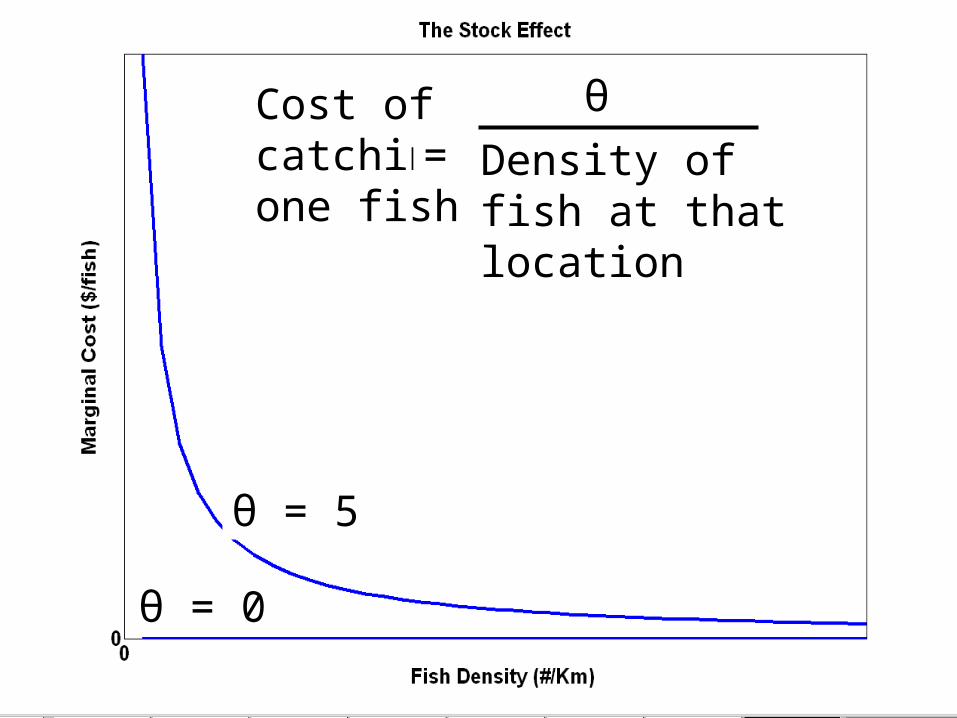
θ = 5
θ = 0
Cost of catching one fish
= Density of fish at that location
θ

θ = 5
θ = 0
Bottom line for fishermen:
Profit = Revenue - cost
Cost of catching one fish
= Density of fish at that location
θ

θ = 20
θ = 0
Bottom line for fishermen:
Profit = Revenue - cost
Cost of catching one fish
= Density of fish at that location
θ

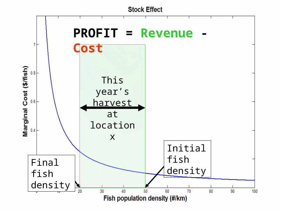
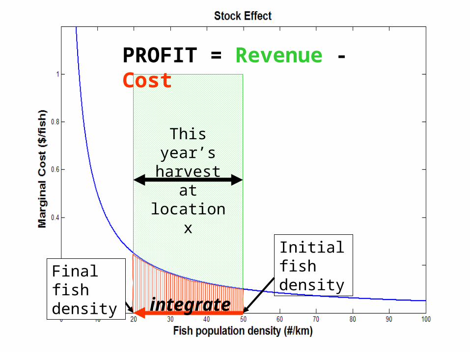
PROFIT = Revenue - Cost
Initial fish density
Final fish density
This year’s harvest at location x

integrate
PROFIT = Revenue - Cost
Final fish density
Initial fish density
This year’s harvest at location x

Incorporating Density Dependence
Post-dispersal: )Hc(Ao
tx
tx
txeRR
sy'all
txyx
ty
ty
tx
tx
tx
tx
1tx R)FLKH(A)HM(AHAA
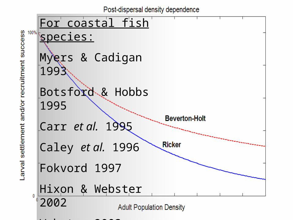
Larva settlement and/or recruitment success increases with decreasing adult population density at that location.

For coastal fish species:
Myers & Cadigan 1993
Botsford & Hobbs 1995
Carr et al. 1995
Caley et al. 1996
Fokvord 1997
Hixon & Webster 2002
Webster 2003
Skajaa et al. In Prep.

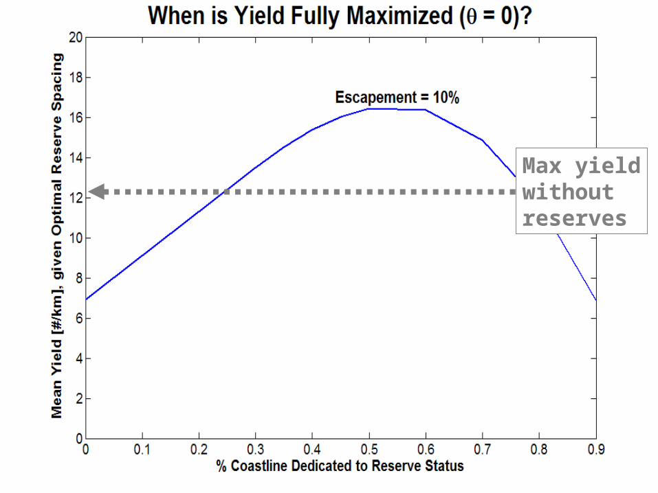
Including stock effect does not influence optimal reserve design
Reserve design that maximizes population density in fishery area:
Maximizes harvest
Minimizes cost of fishing, thereby maximizing profit


0 500 1000 15000
10
20
30
40
50Optimal Reserve Spacing
Distance between reserve centers [km]
Mea
n H
arv
est
Den
sity
[#
fis
h/k
m]
Dd = 100 kmDd = 200 kmDd = 300 km
Reserve = 50% of the coastline
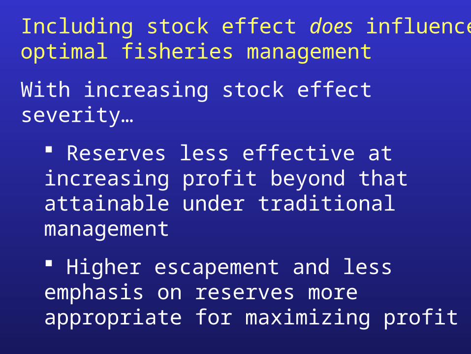
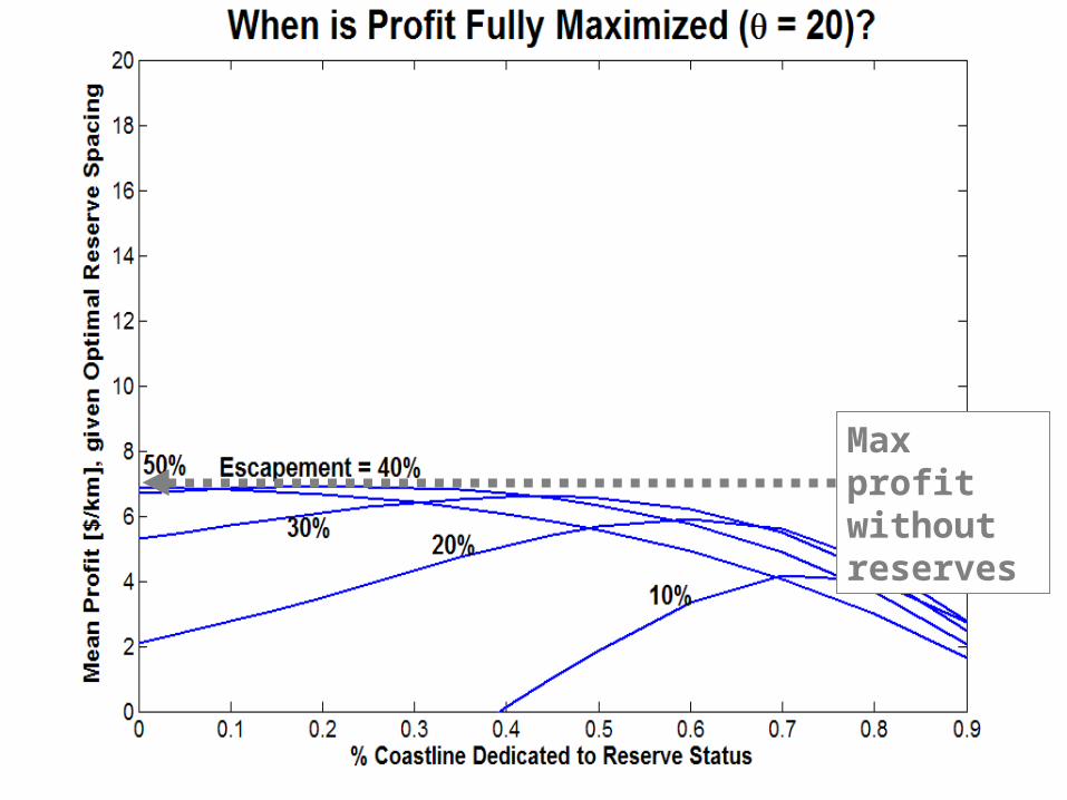
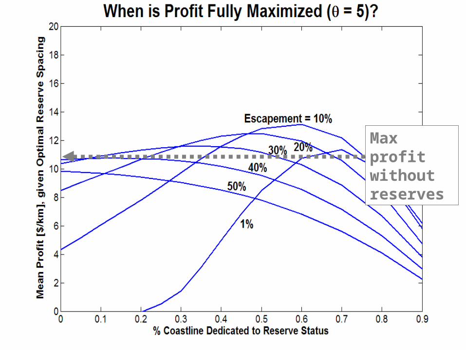
Including stock effect does influence optimal fisheries management
With increasing stock effect severity…
Reserves less effective at increasing profit beyond that attainable under traditional management
Higher escapement and less emphasis on reserves more appropriate for maximizing profit

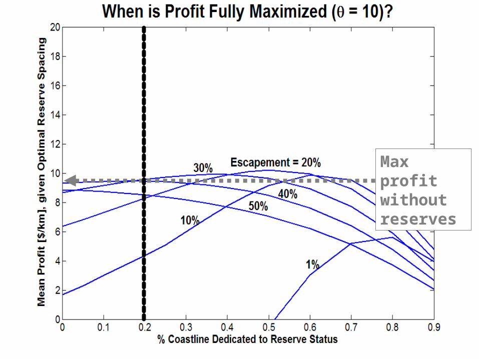
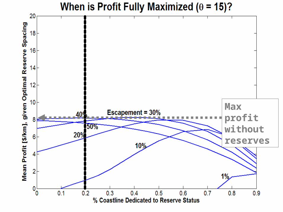
Max yield without reserves

Max profit without reserves

Max profit without reserves

Max profit without reserves
Max profit without reserves
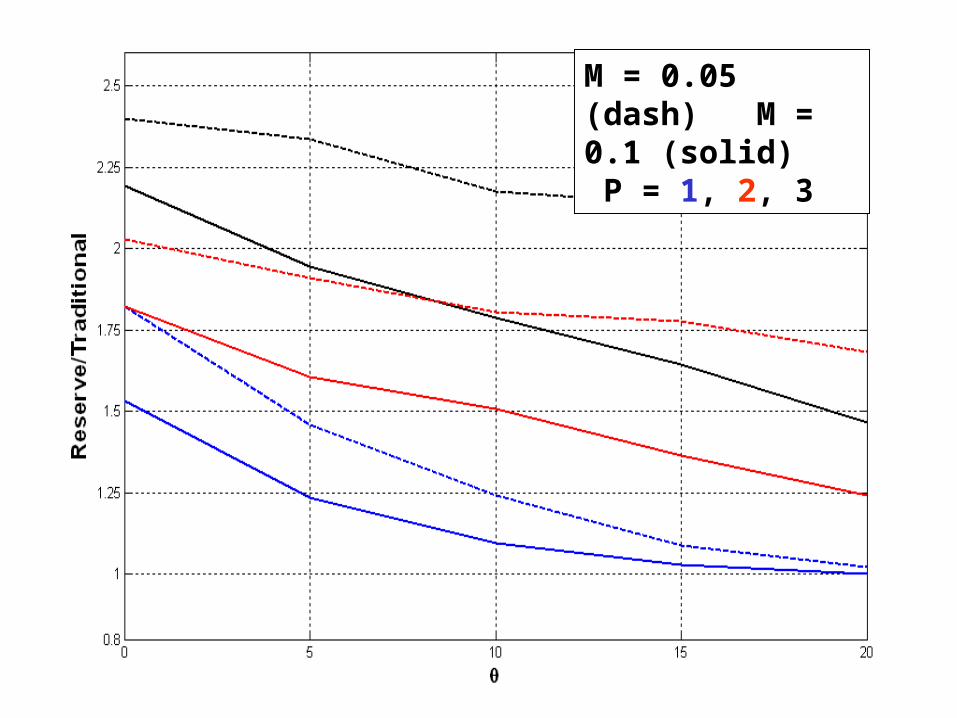
M = 0.05 (dash) M = 0.1 (solid) P = 1, 2, 3

Cost of fishing: Low Cost of fishing: Moderate
Cost of fishing: Higher Cost of fishing: Highest

Max profit without reserves
Max profit without reserves
Max profit without reserves

Max profit without reserves

Reserves = 20% of the coastline (M = 0.1, P = 1)
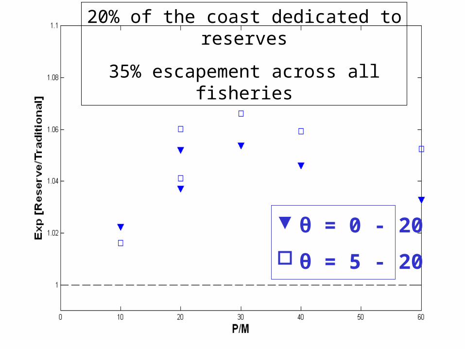
θ = 0 - 20
θ = 5 - 20
20% of the coast dedicated to reserves
35% escapement across all fisheries

θ = 0 - 20
θ = 5 - 20
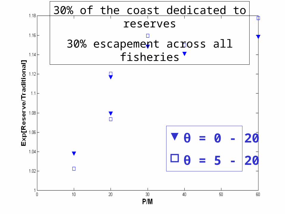
30% of the coast dedicated to reserves
30% escapement across all fisheries

θ = 0 - 20
θ = 5 - 20
40% of the coast dedicated to reserves
30% escapement across all fisheries

θ = 0 - 20
θ = 5 - 20
50% of the coast dedicated to reserves
30% escapement across all fisheries

Reserves = 60% of the coastline

Reserves = 60% of the coastline

60% of the coast dedicated to reserves
θ% escapement across all fisheries
θ = 0 - 20
θ = 5 - 20

Options for fishery management
• Traditional
• No reserves, & high escapement levels (34 - 47% K) individually set for each fishery
• Moderately difficult to enforce
• Mix
• 20 – 50% coast in reserves, & ~30% escapement across all fisheries
• Equivalent/enhanced profit; moderately difficult to enforce
• Reserve
• 60% coast in reserves, & no regulation of escapement
• Equivalent/much enhanced profit; simple to enforce

University of California – Santa Barbara
National Science Foundation
Coastal Environmental Quality Initiative
The Canon National Parks Science Scholars Program
THANK YOU!!

FISHING FOR PROFIT, NOT FISH: AN ECONOMIC
ASSESSMENT OF MARINE RESERVE EFFECTS ON
FISHERIES
Crow White, Bruce Kendall, Dave Siegel, and Chris Costello University of California – Santa Barbara

Compared to traditional (open access) management…
…reserves maintain yields:
▪ Hastings and Botsford 1999
…reserves enhance yield:
▪ Gerber et al. 2003 (a review)
▪ Neubert 2003
▪ Gaylord et al. 2005

θ = 5
θ = 0
Cost of catching one fish
= Density of fish at that location
θ

θ = 5
θ = 0
Bottom line for fishermen:
Profit = Revenue - cost
Cost of catching one fish
= Density of fish at that location
θ

θ = 20
θ = 0
Bottom line for fishermen:
Profit = Revenue - cost
Cost of catching one fish
= Density of fish at that location
θ

No Fishin
g

For coastal fish species:
Myers & Cadigan 1993
Botsford & Hobbs 1995
Carr et al. 1995
Caley et al. 1996
Fokvord 1997
Hixon & Webster 2002
Webster 2003
Skajaa et al. In Prep.

sy'all
txyx
ty
ty
tx
tx
tx
tx
1tx R)FLKH(A)HM(AHAA
An integro-difference model describing coastal fish population dynamics:
Adult abundance at location x during time-step t+1
Number of adults
harvested
Natural mortality of adults that
escaped being harvested
Fecundity
Larval survival
Larval dispersal (Gaussian)(Siegel et al. 2003)
Larval recruitment at x
Number of larvae that successfully recruit to location x

Incorporating Density Dependence
Post-dispersal: )Hc(Ao
tx
tx
txeRR
sy'all
txyx
ty
ty
tx
tx
tx
tx
1tx R)FLKH(A)HM(AHAA
Larva settlement and/or recruitment success increases with decreasing adult population density at that location.

Incorporating Density Dependence
Post-dispersal: )Hc(Ao
tx
tx
txeRR
sy'all
txyx
ty
ty
tx
tx
tx
tx
1tx R)FLKH(A)HM(AHAA
Larva settlement and/or recruitment success increases with decreasing adult population density at that location.
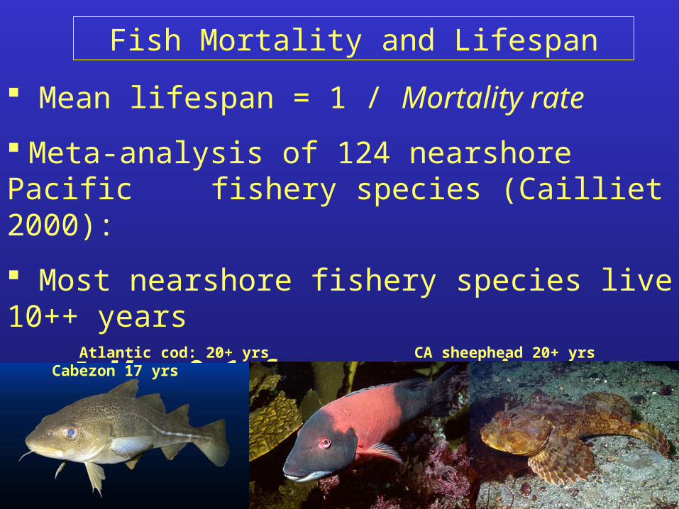
Mean lifespan = 1 / Mortality rate
Meta-analysis of 124 nearshore Pacific fishery species (Cailliet 2000):
Most nearshore fishery species live 10++ years
M < 0.1 for most species
Fish Mortality and Lifespan
Atlantic cod: 20+ yrs CA sheephead 20+ yrs Cabezon 17 yrs
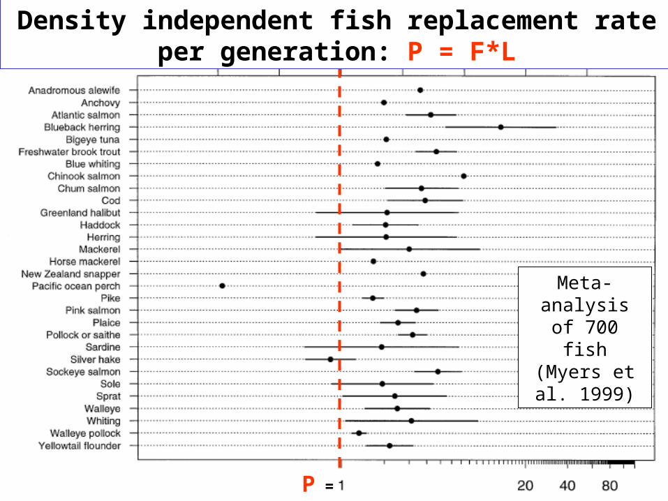
P =
Density independent fish replacement rate per generation: P = F*L
Meta-analysis of
700 fish (Myers et al.
1999)

Mean larval dispersal distance

To maximize profits, should reserves be…
…few and large,
What is the optimal reserve design?
…or many and small?
SLOSS debate
PROFIT = Revenue - Cost
Initial fish density
Final fish density
This year’s harvest at location x
integrate
PROFIT = Revenue - Cost
Final fish density
Initial fish density
This year’s harvest at location x

FEW LARGE RESERVES
SEVERAL SMALL RESERVES

Scale bar = 100 km

Scale bar = 100 km

Scale bar = 100 km


0 500 1000 15000
10
20
30
40
50Optimal Reserve Spacing
Distance between reserve centers [km]
Mea
n H
arv
est
Den
sity
[#
fis
h/k
m]
Dd = 100 kmDd = 200 kmDd = 300 km
Reserve = 50% of the coastline


Max yield without reserves

Max yield without reserves

Max yield without reserves
Max profit without reserves

Max profit without reserves

Max profit without reserves

Max profit without reserves

M = 0.1 (solid) P = 1

M = 0.05 (dash) M = 0.1 (solid) P = 1

M = 0.05 (dash) M = 0.1 (solid) P = 1, 2, 3

Cost of fishing: Low Cost of fishing: Moderate
Cost of fishing: Higher Cost of fishing: Highest

12 reserves constituting ~20% of the C.I. coastline

MPA process along the central CA coast.
Deliberating dedicating ~20% of the coast to a network of ~30 reserves(Pending approval by CDFG and Gov. Szchchweschcwchchcnggchcerrrr)

Georges Bank and two nearby reserves constitute
~20-30% of regional groundfish habitat (Murawski 2000)

Max profit without reserves

Max profit without reserves

Max profit without reserves

Max profit without reserves

Max profit without reserves

Reserves = 20% of the coastline (M = 0.1, P = 1)

θ = 0 - 20
θ = 5 - 20
20% of the coast dedicated to reserves
35% escapement across all fisheries

θ = 0 - 20
θ = 5 - 20
20% of the coast dedicated to reserves
35% escapement across all fisheries
θ = 0 - 20
θ = 5 - 20
30% of the coast dedicated to reserves
30% escapement across all fisheries

θ = 0 - 20
θ = 5 - 20
40% of the coast dedicated to reserves
30% escapement across all fisheries

θ = 0 - 20
θ = 5 - 20
50% of the coast dedicated to reserves
30% escapement across all fisheries

Max profit without reserves
Max profit without reserves
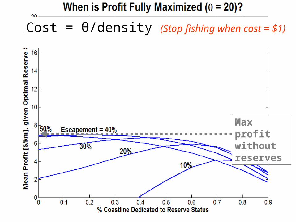
Cost = θ/density (Stop fishing when cost = $1)

Max profit without reserves
Cost = θ/density (Stop fishing when cost = $1)
Escapement = % of virgin K (K = 100)

Max profit without reserves
Cost = θ/density (Stop fishing when cost = $1)
Escapement = % of virgin K (K = 100)
Zero-profit escapement level = θ/K = 20%

Max profit without reserves
Cost = θ/density (Stop fishing when cost = $1)
Escapement = % of virgin K (K = 100)
Zero-profit escapement level = θ/K = 20%

Max profit without reserves
θ/K = 15/100 = 15%

Max profit without reserves
θ/K = 15/100 = 15%

Max profit without reserves
θ/K = 10/100 = 10%
10%

Max profit without reserves
θ/K = 5/100 = 5%
10%

Reserves = 60% of the coastline

Reserves = 60% of the coastline

60% of the coast dedicated to reserves
θ% escapement across all fisheries
θ = 0 - 20
θ = 5 - 20

60% of the coast dedicated to reserves
θ% escapement across all fisheries
θ = 0 - 20
θ = 5 - 20

Summary 1. Profit is bottom line for fishermen and fisheries.
2. Fishery yield and profit maximized via…
A small proportion of the coastline in reserves
…A variety of reserve spacing options.
A large proportion of the coastline in reserves
…Several small or few medium-sized reserves.

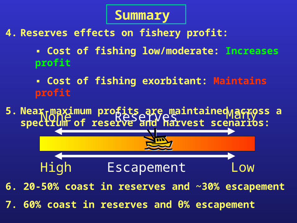
Summary 4. Reserves effects on fishery profit:
▪ Cost of fishing low/moderate: Increases profit
▪ Cost of fishing exorbitant: Maintains profit

Summary 4. Reserves effects on fishery profit:
▪ Cost of fishing low/moderate: Increases profit
▪ Cost of fishing exorbitant: Maintains profit
5. Near-maximum profits are maintained across a spectrum of reserve and harvest scenarios:ReservesNone Many
EscapementHigh Low

Summary 4. Reserves effects on fishery profit:
▪ Cost of fishing low/moderate: Increases profit
▪ Cost of fishing exorbitant: Maintains profit
5. Near-maximum profits are maintained across a spectrum of reserve and harvest scenarios:ReservesNone Many
EscapementHigh Low6. 20-50% coast in reserves and ~30% escapement
7. 60% coast in reserves and θ% escapement

sy'all
txyx
ty
ty
tx
tx
tx
tx
1tx R)FLKH(A)HM(AHAA
An integro-difference model describing coastal fish population dynamics:
Adult abundance at location x during time-step t+1
Number of adults
harvested
Natural mortality of adults that
escaped being harvested
Fecundity
Larval survival
Larval dispersal (Gaussian)(Siegel et al. 2003)
Larval recruitment at x
Number of larvae that successfully recruit to location x

Smooth, Gaussian larval dispersal kernel
Based on MCMC particle simulations in a 2-D field characterized by flow velocities obtained from buoys and drifters along the central CA coast.
Siegel et al. 2003

Stochastic larval dispersal kernel
Heterogeneous dispersal pattern due to stochastic ocean flow field dynamics
Siegel et al. 2003
Delivery of larval “packet”

SeaWiFS - NASA
California Current
San Francisco
Santa Barbara
Los Angeles

SeaWiFS - NASA
California Current
San Francisco
Santa Barbara
Los Angeles

With fish abundance
Nishimoto & Washburn (2002)
• Elwood Beach

SETTLEMENT TIME SERIES
160 180 200 220 240 260 280 300 3200
10
20
30
40
50
60
70
JD 2001
# se
ttle
rs/d
eplo
ymen
tEllwood Invert Setttlment Time Series
Mytilus Clams (excl razor & HIAARC) any marine snail (excl. veligers, limp)Limpet species Snail veliger any seastar Hiatella arctica
Data Courtesy - PISCO [UCSB]

A STIRRED OCEAN
• Larval dispersal is stochastic driven by turbulent “eddies”– Not smooth diffusion processes
• Makes recruitment and stock distribution predictions challenging

Estimate stochastic dispersal patterns: BIO-PHYSICAL SIMULATIONS
• Simulate coastal circulation processes in California current system– Using ROMS (Rutgers)
– Driven by real data• Buoys and transects
• Release & track “larvae”• Obtain connectivity Mean wind
Mean offshore current at surface due to Coriolis Force
- Creates upwelling

Estimate stochastic dispersal patterns: BIO-PHYSICAL SIMULATIONS
TARGET AREA:• Central California
– Relatively straight coast
– Wind is dominant• Equatorward
Mean windMean offshore current at surface due to Coriolis Force
- Creates upwelling

IDEALIZED SIMULATIONTop view
Alongshore pressure gradient obtained from observation data
Poleward geostrophic force applied as an
external force
Stochastic wind stressestimated from observation data
Predominantly southward
Side viewPeriodic
PeriodicC
oast
= W
all
Ope
n Poleward

°C

SIMULATION VALIDATION: MEAN TEMPERATURE
Simulation
• Shows good agreement with CalCOFI seasonal mean (Line 70)
CalCOFI seasonal mean
°C °C

SIMULATION VALIDATION:LAGRANGIAN STATISTICS
Time scale Length scale Diffusivityzonal/meridional zonal/meridional zonal/meridional
2.7/2.9 days 29/31 km 4.0/4.3 x107 cm2/s
2.9/3.5 days 32/38 km 4.3/4.5 x107 cm2/sSurface drifter data(Swenson & Niiler)
Simulation data
Data set
• Shows good agreement with surface drifter data

ADD LARVAE
• Release many (105) Lagrangian particles as model larvae
• Pattern after rocky reef fish– Larvae are released daily for 90 days, uniformly
distributed in habitat – Settlement competency window = day 20-40 – Nearshore habitat = waters within 10 km from
the coast
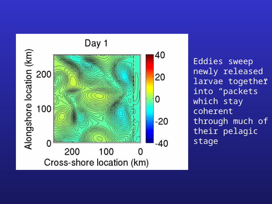
Eddies sweep newly released larvae together into “packets” which stay coherent through much of their pelagic stage

ALL larvaeRed dots = settling larvae
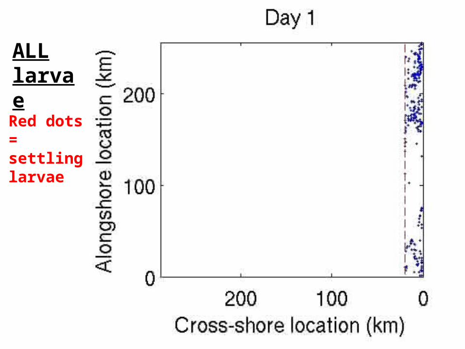
ALL larvaeRed dots = settling larvae

DEPARTURE, ARRIVAL& CONNECTIVITY
• Connectivity is inherently heterogeneous• No bathymetric or coastline variability necessary
x
'x
nxxK ',

THREE MORE REALIZATIONS
• Different realizations -> different connectivity

THREE MORE REALIZATIONS
…
• Connectivity is not diffusive

DISPERSAL KERNELSample dispersal kernel
(from a 10-km subpopulation)Ensemble averaged
(& normalized)
Gaussian fit

Stochastic settlement patterns will be most pronounced for species with…
• Short and periodic spawning seasons
• Late-stage settlement competency windows
• Little/no active swimming behaviors

Population Dynamics Implications of Stochastic Dispersal Kernel
• Habitat connectivity on annual scales is uncertain (“flow-induced uncertainty”)– Hotspots shift from year to year
– Habitat connectivity is heterogeneous & intermittent & NOT diffusive
• Even if coastline and bathymetry is smooth
– Spatial variance in hotspots likely reduced by inclusion of variable bathymetry and coastal contours
• Modeling implications– Must account for massive, local recruitment events
• Add larvae-on-larvae density dependence to represent competition for limited settlement niches at a site

• Even with perfect knowledge of current stock distribution & productivity– Recruitment and future stock predictions uncertain
• Difficult to assess appropriate escapement level– High potential for over-exploitation at recruitment-failure location
• Reliance on reserve management more practical– Network of reserves provide many potential sources
• Consequences of over-exploitation reduced due to reserves
– Fisheries can track locate and exploit “hot spots”• Fishermen can act in real time (managers have to forecast)
Fisheries Management Implications of Stochastic Dispersal Kernel
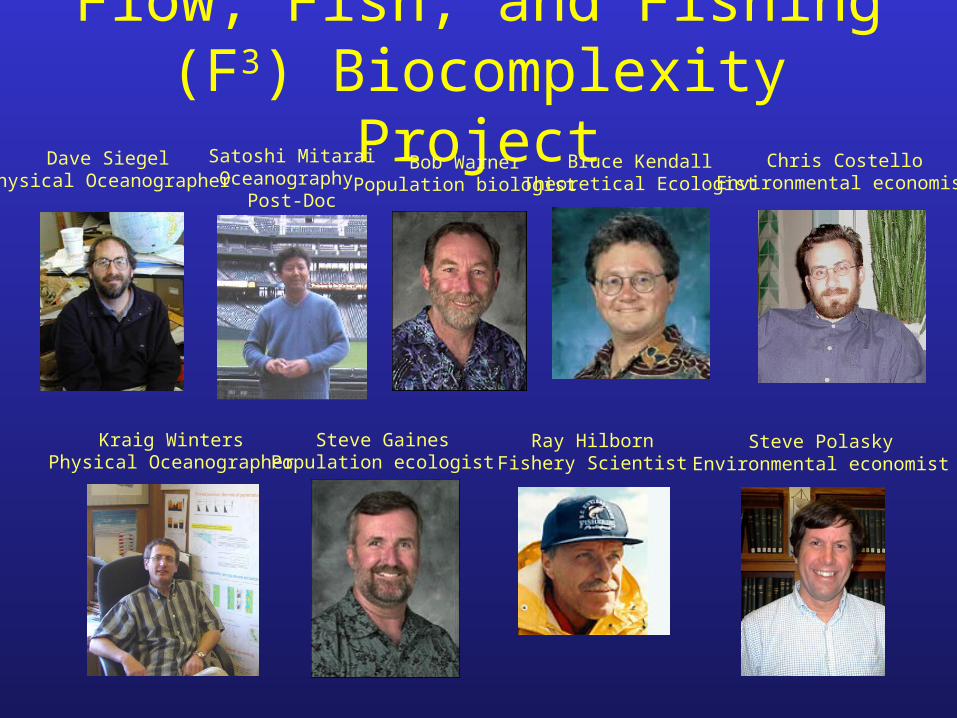
Flow, Fish, and Fishing (F3) Biocomplexity Project
Dave SiegelPhysical Oceanographer
Kraig WintersPhysical Oceanographer
Bob WarnerPopulation biologist
Steve PolaskyEnvironmental economist
Bruce KendallTheoretical Ecologist
Ray HilbornFishery Scientist
Chris CostelloEnvironmental economist
Steve GainesPopulation ecologist
Satoshi MitaraiOceanography
Post-Doc
University of California – Santa Barbara
National Science Foundation
Coastal Environmental Quality Initiative
The Canon National Parks Science Scholars Program
THANK YOU!!


SIDE VIEW ALL LARVAE
Red dots = settling larvae

SIDE VIEW ALL LARVAE
Red dots = settling larvae

Effects of age/stage structure on fish population and fishery dynamics
Per capita production increases (exponentially) with age.
But K (#fish/km) will decrease…

25% of the coast dedicated to reserves
30% escapement across all fisheries
θ = 0 - 20
θ = 5 - 20