FIRST-ORDER ORDINARY DIFFERENTIAL EQUATIONS

G(x, y, y′) = 0

♦ in normal form:

y′ = F (x, y)

♦ in differential form:

M(x, y)dx+N(x, y)dy = 0

• Last time we discussed first-order linear ODE: y′ + q(x)y = h(x).We next consider first-order nonlinear equations.

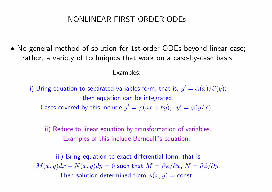
NONLINEAR FIRST-ORDER ODEs

• No general method of solution for 1st-order ODEs beyond linear case;rather, a variety of techniques that work on a case-by-case basis.

Examples:

i) Bring equation to separated-variables form, that is, y′ = α(x)/β(y);

then equation can be integrated.

Cases covered by this include y′ = ϕ(ax+ by); y′ = ϕ(y/x).

ii) Reduce to linear equation by transformation of variables.

Examples of this include Bernoulli’s equation.

iii) Bring equation to exact-differential form, that is

M(x, y)dx+N(x, y)dy = 0 such that M = ∂φ/∂x, N = ∂φ/∂y.

Then solution determined from φ(x, y) = const.

• Useful reference for the ODE part of this course(worked problems and examples)

Schaum’s Outline Series

Differential Equations

R. Bronson and G. CostaMcGraw-Hill (Third Edition, 2006)

♦ Chapters 1 to 7: First-order ODE.

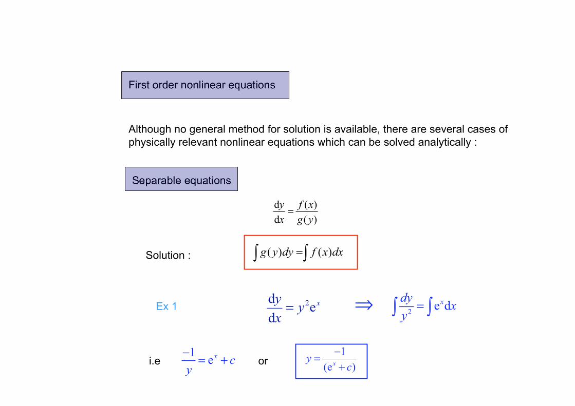
First order nonlinear equations

Although no general method for solution is available, there are several cases of

physically relevant nonlinear equations which can be solved analytically :

Separable equations

d ( )

d ( )

y f x

x g y=

( ) ( )g y dy f x dx=! !Solution :

2de

d

xyy

x=Ex 1

2e dxdyx

y=! " "

1exc

y

!= +i.e

1

(e )xy

c

!=

+or

Almost separable equations

d( )

d

yf ax by

x= +

z ax by= +dd

d d

yz

x xa b= +Change variables :

1d

( ( ))x z

a bf z= .

+!d

( )d

za bf z

x= + !

2d( 4 )

d

yx y

x= ! + 4z y x= !

2d d4 4

d d

z yz

x x! = " + = "

1 24 2ln( ) Cz

zx

!

+= +

4

4

(1 e )

(1 e )4 2

x

x

k

ky x

+

!" = +

Ex 2

k a constant

z ax by= +

d( )

d

za bf z

x= + !

d( )

d

yf y x

x= / .

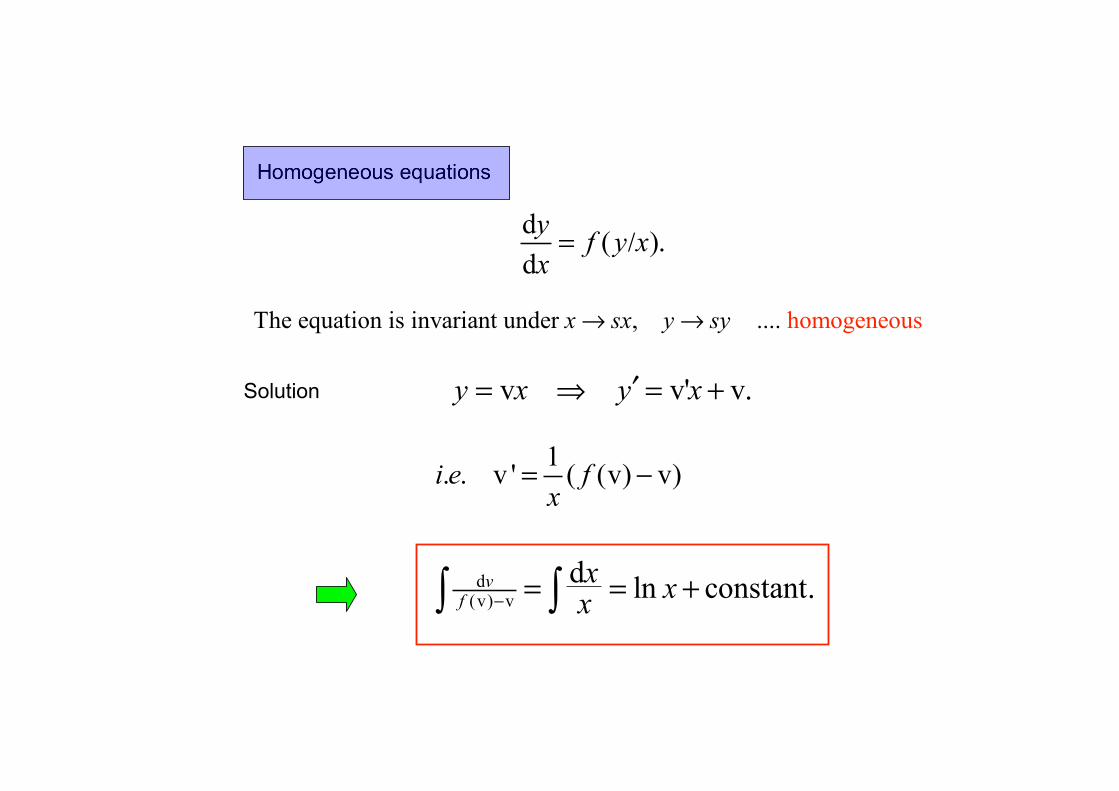
Homogeneous equations

The equation is invariant under , .. h.. omogeneousx sx y sy! !

v v' vy x y x!= " = + .Solution

d(v) v

d ln constantv

f

xx

x! = = + ." "

1. . v ' ( (v) v)i e f

x= !

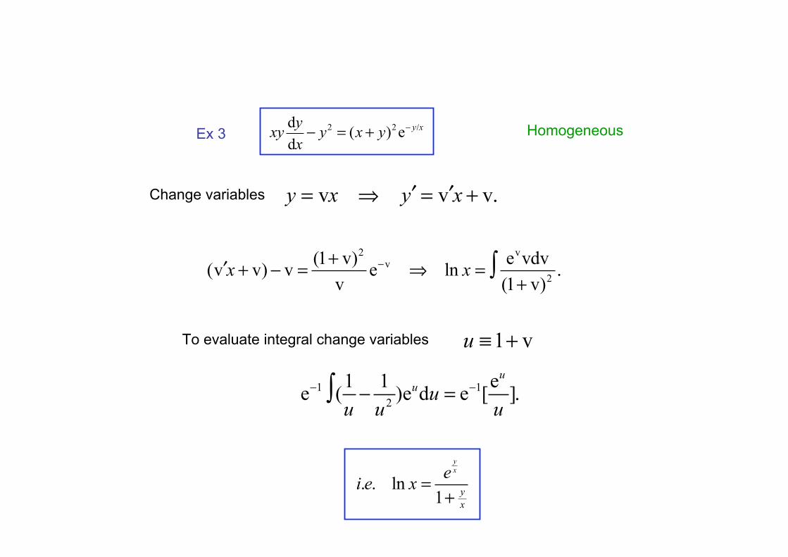
2 2d( ) e

d

y xyxy y x y

x

! /! = +Ex 3

2 vv

2

(1 v) e vdv(v v) v e ln

v (1 v)x x

!+" + ! = # = .

+$

1 vu ! +

1 1

2

1 1 ee ( )e d e [ ]

u

uu

u u u

! !! = ."

v v vy x y x! != " = + .Change variables

To evaluate integral change variables

. . ln1

y

x

y

x

ei e x =

+

Homogeneous

Homogeneous but for constants

2 1

2

dy x y

dx x y

+ +=

+ +

' , 'x x a y y b= + = +' ' ' '

.' '

dy dy dy dx dy

dx dx dx dx dx! = = =

' ' 2 ' 1 2

' ' ' 2

dy x y a b

dx x y a b

+ + + +=

+ + + +

1 2 0a b+ + =

2 0a b+ + =

3, 1a b= ! =

' ' 2 '

' ' '

dy x y

dx x y

+=

+Homogeneous

The Bernoulli equation

d( ) ( ) , 1

d

nyP x y Q x y n

x+ = !

To solve, change variable to 1 n

z y!

= (1 ) ndz dyn y

dx dx

!" = !

(1 ) ( ) (1 ) ( )dz

n P x z n Q xdx

+ ! = !Gives the equation

Ex 42/3

'y y y+ =1 1/3n

z y y!

= = 1

3'3

zz! + =

x/3Integrating factor e

1/ 3 /31

xz y ce

!= = +

/ 3 /3/ 3

x xze e dx! = "

1st order Linear

1st order linear

Exercise:

Solve the equation 2 y ′ = y/x+ x2/ywith initial condition y(1) = 2.

• This equation is Bernoulli with n = −1.

• Set z = y2. Then z′ − z/x = x2.

• Integrating factor I(x) = 1/x

⇒ z(x) = x [

∫

dx x2/x+ const.] = x3/2 + const. x

Thus y = z1/2 = ±√

x3/2 + const. x

• Initial condition y(1) = 2

⇒ y(x) =

√

x3 + 7x

2

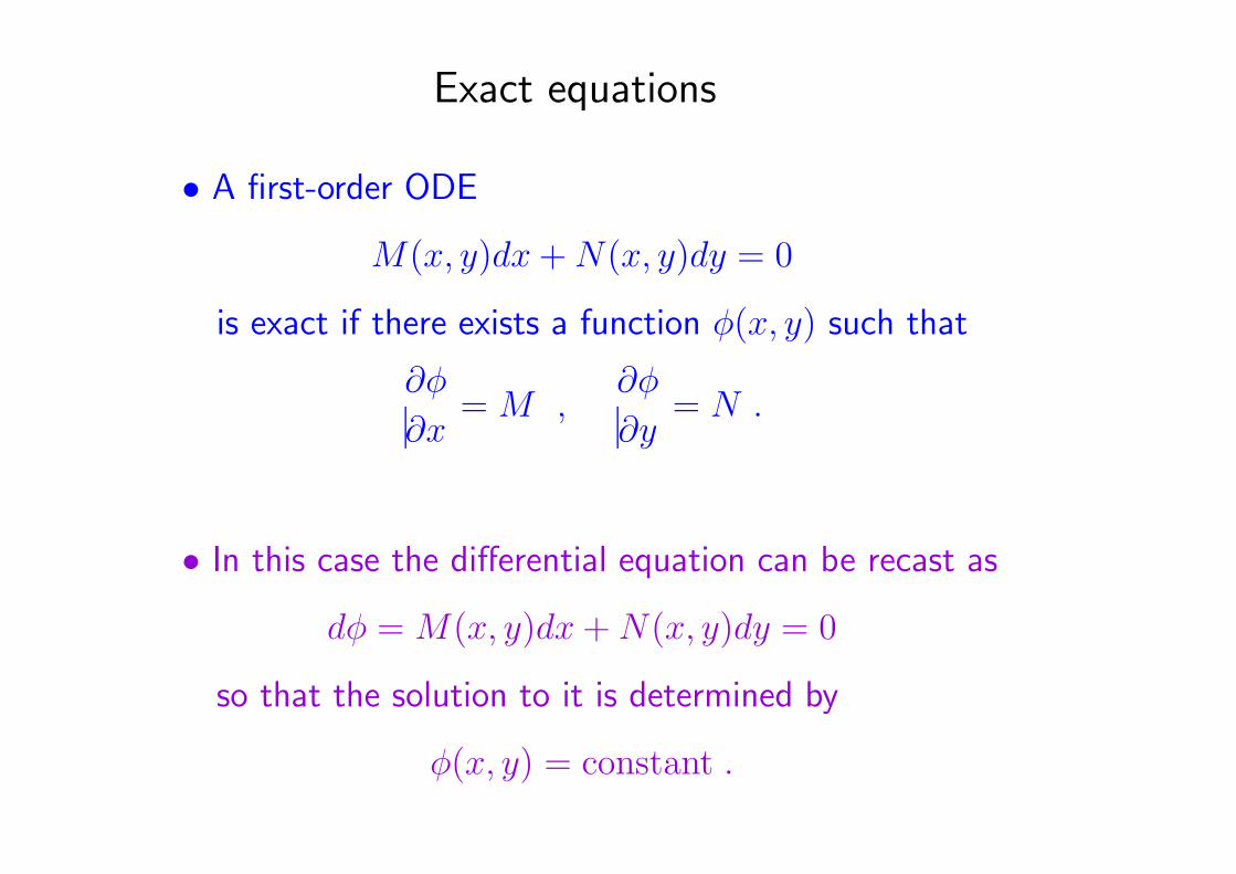
Exact equations

• A first-order ODE

M(x, y)dx+N(x, y)dy = 0

is exact if there exists a function φ(x, y) such that

∂φ

∂x= M ,

∂φ

∂y= N .

• In this case the differential equation can be recast as

dφ = M(x, y)dx+N(x, y)dy = 0

so that the solution to it is determined by

φ(x, y) = constant .

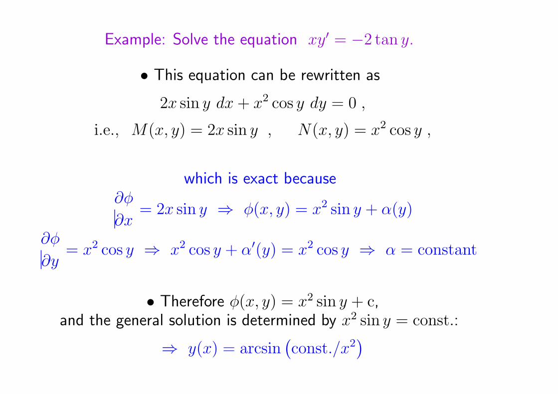
Example: Solve the equation xy′ = −2 tan y.

• This equation can be rewritten as

2x sin y dx+ x2 cos y dy = 0 ,

i.e., M(x, y) = 2x sin y , N(x, y) = x2 cos y ,

which is exact because∂φ

∂x= 2x sin y ⇒ φ(x, y) = x2 sin y + α(y)

∂φ

∂y= x2 cos y ⇒ x2 cos y + α′(y) = x2 cos y ⇒ α = constant

• Therefore φ(x, y) = x2 sin y + c,and the general solution is determined by x2 sin y = const.:

⇒ y(x) = arcsin(

const./x2)

DIFFERENTIAL EQUATIONS AND FAMILIES OF CURVES

• General solution of a first-order ODE y′ = f(x, y)

contains an arbitrary constant: y = (x, c)

⊲ one curve in x, y plane for each value of c⊲ general solution can be thought of as one-parameter family of curves

Example: y′ = −x/y.

separable equation ⇒

∫

y dy = −

∫

x dx ⇒ y2/2 = −x2/2 + c

i.e., x2 + y2 = constant : family of circles centered at origin

Fig.1

x

y

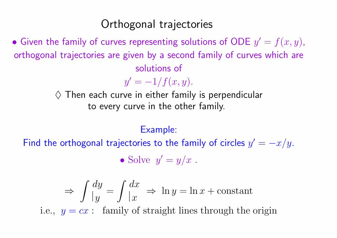
Orthogonal trajectories

• Given the family of curves representing solutions of ODE y′ = f(x, y),

orthogonal trajectories are given by a second family of curves which are

solutions of

y′ = −1/f(x, y).

♦ Then each curve in either family is perpendicularto every curve in the other family.

Example:

Find the orthogonal trajectories to the family of circles y′ = −x/y.

• Solve y′ = y/x .

⇒

∫

dy

y=

∫

dx

x⇒ ln y = ln x+ constant

i.e., y = cx : family of straight lines through the origin

a) Find the family of curves corresponding to solutions of the ODE

y′ = (y2 − x2)/(2xy).

b) Find the orthogonal trajectories to the above family of curves.

• homogeneous equation y′ = f(y/x) with f(y/x) = (y/x− x/y)/2

solvable by y→v = y/x and separation of variables

⇒ x2 + y2 = cx : family of circles tangent to y − axis at 0

y

x

Fig.2

• orthogonal trajectories found by solving y′ = −2xy/(y2 − x2)

⇒ x2 + y2 = ky : family of circles tangent to x− axis at 0

EXPLOITING FIRST-ORDER METHODS TO TREAT EQUATIONS OF

HIGHER ORDER IN SPECIAL CASES

♣ y not present in 2nd-order equation F (x, y, y′, y′′) = 0

⇒ setting y′ = q yields 1st-order equation for q(x).

♣ x not present in 2nd-order equation F (x, y, y′, y′′) = 0

⇒ setting y′ = q, y′′ = dq/dx = q(dq/dy) yields G(y, q, dq/dy) = 0.

2

x

y

T

θT

s

Example: homogeneous, flexible chain hanging under its own weight

ρ = linear mass density

Using Newton’s law, the shape y(x) of the chain obeys the 2nd−order nonlinear differential equation

y = a 1 + (y )2 , a ρ g / T

Setting y = q q = a 1 + q

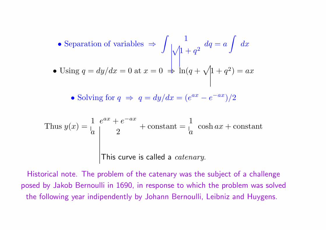
• Separation of variables ⇒

∫

1√

1 + q2dq = a

∫

dx

• Using q = dy/dx = 0 at x = 0 ⇒ ln(q +√

1 + q2) = ax

• Solving for q ⇒ q = dy/dx = (eax − e−ax)/2

Thus y(x) =1

a

eax + e−ax

2+ constant =

1

acosh ax+ constant

This curve is called a catenary.

Historical note. The problem of the catenary was the subject of a challenge

posed by Jakob Bernoulli in 1690, in response to which the problem was solved

the following year indipendently by Johann Bernoulli, Leibniz and Huygens.

Summary

♦ No general method of solution for 1st-order ODEs beyond linear case;

rather, a variety of techniques that work on a case-by-case basis.

Main guiding criteria:• methods to bring equation to separated-variables form

• methods to bring equation to exact differential form

• transformations that linearize the equation

♦ 1st-order ODEs correspond to families of curves in x, y plane⇒ geometric interpretation of solutions

♦ Equations of higher order may be reduceable to first-order problems inspecial cases — e.g. when y or x variables are missing from 2nd order

equations