ordinary differential equationspages.jh.edu/~motn/relevantnotes/usingmatlab_ode.pdf · ordinary...
TRANSCRIPT
Representing Problems . . . . . . . . . . . . . . . 8-5
ODE Solvers . . . . . . . . . . . . . . . . . . . . 8-10
Creating ODE Files . . . . . . . . . . . . . . . . . 8-14
Improving Solver Performance . . . . . . . . . . . 8-17
Examples: Applying the ODE Solvers . . . . . . . . . 8-34
8
Ordinary Differential EquationsQuick Start . . . . . . . . . . . . . . . . . . . . 8-3
8 Ordinary Differential Equations
8-2
This chapter describes how to use MATLAB to solve initial value problems of ordinary differential equations (ODEs) and differential algebraic equations (DAEs). It discusses how to represent initial value problems (IVPs) in MATLAB and how to apply MATLAB’s ODE solvers to such problems. It explains how to select a solver, and how to specify solver options for efficient, customized execution. This chapter also includes a troubleshooting guide in the Questions and Answers section and extensive examples in the Examples: Applying the ODE Solver section.
Category Function Description
Ordinary differential equation solvers
ode45 Nonstiff differential equations, medium order method.
ode23 Nonstiff differential equations, low order method.
ode113 Nonstiff differential equations, variable order method.
ode15s Stiff differential equations and DAEs, variable order method.
ode23s Stiff differential equations, low order method.
ode23t Moderately stiff differential equations and DAEs, trapezoidal rule.
ode23tb Stiff differential equations, low order method.
ODE option handling odeset Create/alter ODE OPTIONS structure.
odeget Get ODE OPTIONS parameters.
ODE output functions odeplot Time series plots.
odephas2 Two-dimensional phase plane plots.
odephas3 Three-dimensional phase plane plots.
odeprint Print to command window.
Quick Start
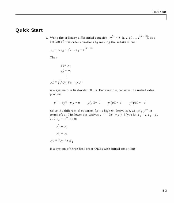
Quick Start1 Write the ordinary differential equation as a
system of first-order equations by making the substitutions
Then
is a system of n first-order ODEs. For example, consider the initial value problem
Solve the differential equation for its highest derivative, writing in terms of t and its lower derivatives . If you let , and , then
is a system of three first-order ODEs with initial conditions
y n( ) f t y y ′ .... y n 1–( ), , , ,( )=
y1 y= y2 y′ ... yn, , y n 1–( )= =,
y1′ y2=
y2′ y3=
.·
yn′ f t y1 y2 ... y, n, , ,( )=
y′′′ 3y′′– y′y 0=– y 0( ) 0= y′ 0( ) 1= y′′ 0( ) 1–=
y′′′y′′′ 3y′′ y′y+= y1 y= y2 y′=,
y3 y′′=
y1′ y2=
y2′ y3=
y3′ 3y3 y2y1+=
8-3
8 Ordinary Differential Equations
8-4
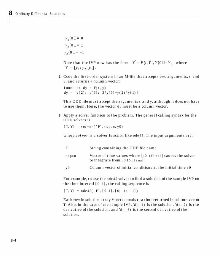
Note that the IVP now has the form , where .
2 Code the first-order system in an M-file that accepts two arguments, t and y, and returns a column vector:
function dy = F(t,y)dy = [y(2); y(3); 3*y(3)+y(2)*y(1)];
This ODE file must accept the arguments t and y, although it does not have to use them. Here, the vector dy must be a column vector.
3 Apply a solver function to the problem. The general calling syntax for the ODE solvers is
[T,Y] = solver(’F’,tspan,y0)
where solver is a solver function like ode45. The input arguments are:
For example, to use the ode45 solver to find a solution of the sample IVP on the time interval [0 1], the calling sequence is
[T,Y] = ode45('F',[0 1],[0; 1; –1])
Each row in solution array Y corresponds to a time returned in column vector T. Also, in the case of the sample IVP, Y(:,1) is the solution, Y(:,2) is the derivative of the solution, and Y(:,3) is the second derivative of the solution.
F String containing the ODE file name
tspan Vector of time values where [t0 tfinal] causes the solver to integrate from t0 to tfinal
y0 Column vector of initial conditions at the initial time t0
y1 0( ) 0=
y2 0( ) 1=
y3 0( ) 1–=
Y′ F t Y,( )= Y 0( ) Y0=,Y y1 y2 y3;;[ ]=
Representing Problems
Representing Problems This section describes how to represent ordinary differential equations as systems for the MATLAB ODE solvers.
The MATLAB ODE solvers are designed to handle ordinary differential equations. These are differential equations containing one or more derivatives of a dependent variable y with respect to a single independent variable t, usually referred to as time. The derivative of y with respect to t is denoted as
, the second derivative as , and so on. Often y(t) is a vector, having elements y1, y2, ... yn.
ODEs often involve a number of dependent variables, as well as derivatives of order higher than one. To use the MATLAB ODE solvers, you must rewrite such equations as an equivalent system of first-order differential equations in terms of a vector y and its first derivative.
Once you represent the equation in this way, you can code it as an ODE M-file that a MATLAB ODE solver can use.
Initial Value Problems and Initial ConditionsGenerally there are many functions y(t) that satisfy a given ODE, and additional information is necessary to specify the solution of interest. In an initial value problem, the solution of interest has a specific initial condition, that is, y is equal to y0 at a given initial time t0. An initial value problem for an ODE is then
If the function is sufficiently smooth, this problem has one and only one solution. Generally there is no analytic expression for the solution, so it is necessary to approximate by numerical means, such as one of the solvers of the MATLAB ODE suite.
Example: The van der Pol EquationAn example of an ODE is the van der Pol equation
y′ y′′
y′ F t y,( )=
y′ F t y,( )=
y t0( ) y0=
F t y,( )
y t( )
8-5
8 Ordinary Differential Equations
8-6
where µ > 0 is a scalar parameter.
Rewriting the SystemTo express this equation as a system of first-order differential equations for MATLAB, introduce a variable y2 such that y1′= y2. You can then express this system as
Writing the ODE FileThe code below shows how to represent the van der Pol system in a MATLAB ODE file, an M-file that describes the system to be solved. An ODE file always accepts at least two arguments, t and y. This simple two line file assumes a value of 1 for µ. y1 and y2 become y(1) and y(2), elements in a two-element vector.
function dy = vdp1(t,y)dy = [y(2); (1–y(1)^2)*y(2)–y(1)];
Note This ODE file does not actually use the t argument in its computations. It is not necessary for it to use the y argument either – in some cases, for example, it may just return a constant. The t and y variables, however, must always appear in the input argument list.
Calling the SolverOnce the ODE system is coded in an ODE file, you can use the MATLAB ODE solvers to solve the system on a given time interval with a particular initial condition vector. For example, to use ode45 to solve the van der Pol equation on time interval [0 20] with an initial value of 2 for y(1) and an initial value of 0 for y(2).
[T,Y] = ode45(’vdp1’,[0 20],[2; 0]);
y1″ µ 1 y12
–( )y1′– y1 0=+
y1′ y2=
y2′ µ 1 y12
–( )y2 y1–=
Representing Problems
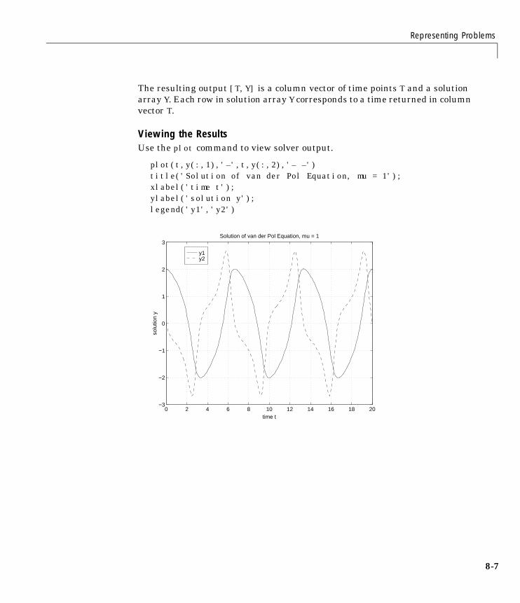
The resulting output [T,Y] is a column vector of time points T and a solution array Y. Each row in solution array Y corresponds to a time returned in column vector T.
Viewing the ResultsUse the plot command to view solver output.
plot(t,y(:,1),'–',t,y(:,2),'– –')title('Solution of van der Pol Equation, mu = 1');xlabel('time t');ylabel('solution y');legend('y1','y2')
0 2 4 6 8 10 12 14 16 18 20−3
−2
−1
0
1
2
3
time t
solu
tion
y
Solution of van der Pol Equation, mu = 1
y1y2
8-7
8 Ordinary Differential Equations
8-8
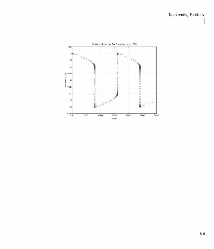
Example: The van der Pol Equation, µ = 1000 (Stiff)
Stiff ODE Problems This section presents a stiff problem. For a stiff problem, solutions can change on a time scale that is very short compared to the interval of integration, but the solution of interest changes on a much longer time scale. Methods not designed for stiff problems are ineffective on intervals where the solution changes slowly because they use time steps small enough to resolve the fastest possible change.
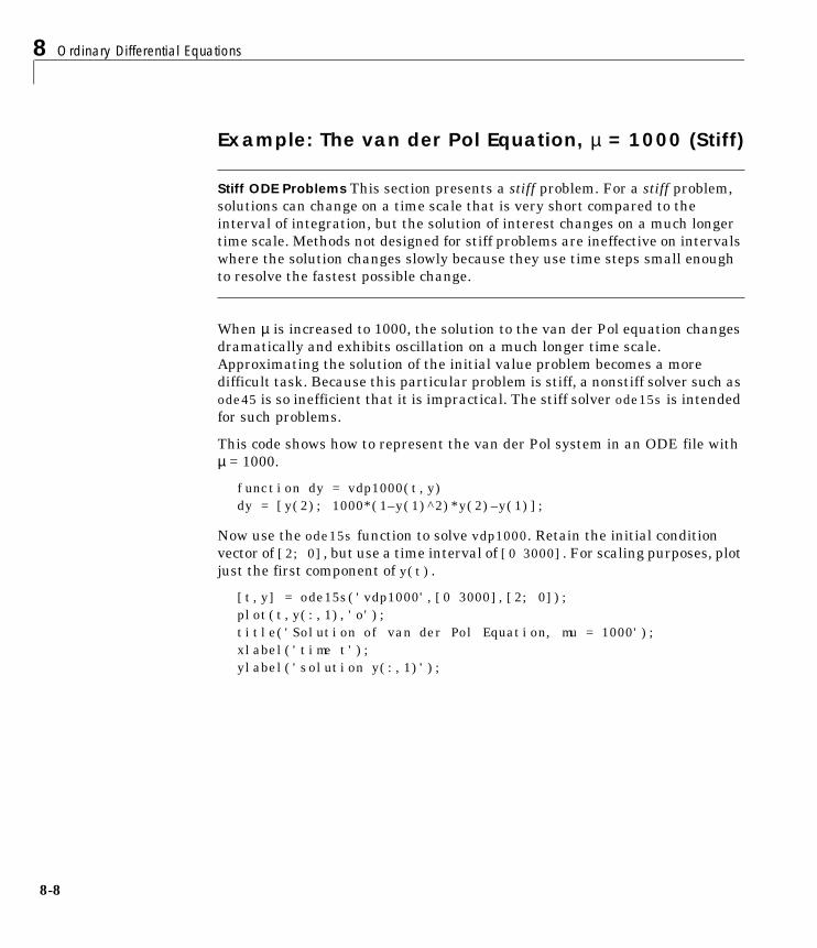
When µ is increased to 1000, the solution to the van der Pol equation changes dramatically and exhibits oscillation on a much longer time scale. Approximating the solution of the initial value problem becomes a more difficult task. Because this particular problem is stiff, a nonstiff solver such as ode45 is so inefficient that it is impractical. The stiff solver ode15s is intended for such problems.
This code shows how to represent the van der Pol system in an ODE file with µ = 1000.
function dy = vdp1000(t,y)dy = [y(2); 1000*(1–y(1)^2)*y(2)–y(1)];
Now use the ode15s function to solve vdp1000. Retain the initial condition vector of [2; 0], but use a time interval of [0 3000]. For scaling purposes, plot just the first component of y(t).
[t,y] = ode15s('vdp1000',[0 3000],[2; 0]);plot(t,y(:,1),'o');title('Solution of van der Pol Equation, mu = 1000');xlabel('time t');ylabel('solution y(:,1)');
Representing Problems
0 500 1000 1500 2000 2500 3000−2.5
−2
−1.5
−1
−0.5
0
0.5
1
1.5
2
2.5
time t
solu
tion
y(:,1
)
Solution of van der Pol Equation, mu = 1000
8-9
8 Ordinary Differential Equations
8-1
ODE SolversThe MATLAB ODE solver functions implement numerical integration methods. Beginning at the initial time and with initial conditions, they step through the time interval, computing a solution at each time step. If the solution for a time step satisfies the solver’s error tolerance criteria, it is a successful step. Otherwise, it is a failed attempt; the solver shrinks the step size and tries again.
This section describes how to represent problems for use with the MATLAB solvers and how to optimize solver performance. You can also use the online help facility to get information on the syntax for any function, as well as information on demo files for these solvers.
Nonstiff SolversThere are three solvers designed for nonstiff problems:
• ode45 is based on an explicit Runge-Kutta (4,5) formula, the Dormand-Prince pair. It is a one-step solver – in computing y(tn), it needs only the solution at the immediately preceding time point, y(tn–1). In general, ode45 is the best function to apply as a “first try” for most problems.
• ode23 is also based on an explicit Runge-Kutta (2,3) pair of Bogacki and Shampine. It may be more efficient than ode45 at crude tolerances and in the presence of mild stiffness. Like ode45, ode23 is a one-step solver.
• ode113 is a variable order Adams-Bashforth-Moulton PECE solver. It may be more efficient than ode45 at stringent tolerances and when the ODE function is particularly expensive to evaluate. ode113 is a multistep solver – it normally needs the solutions at several preceding time points to compute the current solution.
Stiff SolversNot all difficult problems are stiff, but all stiff problems are difficult for solvers not specifically designed for them. Stiff solvers can be used exactly like the other solvers. However, you can often significantly improve the efficiency of the stiff solvers by providing them with additional information about the problem. See “Improving Solver Performance” on page 8-17 for details on how to provide this information, and for details on how to change solver parameters such as error tolerances.
0
ODE Solvers
There are four solvers designed for stiff (or moderately stiff) problems:
• ode15s is a variable-order solver based on the numerical differentiation formulas (NDFs). Optionally it uses the backward differentiation formulas, BDFs, (also known as Gear’s method) that are usually less efficient. Like ode113, ode15s is a multistep solver. If you suspect that a problem is stiff or if ode45 failed or was very inefficient, try ode15s.
• ode23s is based on a modified Rosenbrock formula of order 2. Because it is a one-step solver, it may be more efficient than ode15s at crude tolerances. It can solve some kinds of stiff problems for which ode15s is not effective.
• ode23t is an implementation of the trapezoidal rule using a “free” interpolant. Use this solver if the problem is only moderately stiff and you need a solution without numerical damping.
• ode23tb is an implementation of TR-BDF2, an implicit Runge-Kutta formula with a first stage that is a trapezoidal rule step and a second stage that is a backward differentiation formula of order two. By construction, the same iteration matrix is used in evaluating both stages. Like ode23s, this solver may be more efficient than ode15s at crude tolerances.
ODE Solver Basic SyntaxAll of the ODE solver functions share a syntax that makes it easy to try any of the different numerical methods if it is not apparent which is the most appropriate. To apply a different method to the same problem, simply change the ODE solver function name. The simplest syntax, common to all the solver functions, is
[T,Y] = solver(’F’,tspan,y0)
where solver is one of the ODE solver functions listed previously.
8-11
8 Ordinary Differential Equations
8-1
The input arguments are:
The output arguments are:
Obtaining Solutions at Specific Time PointsTo obtain solutions at specific time points t0, t1, ... tfinal, specify tspan as a vector of the desired times. The time values must be in order, either increasing or decreasing.
Specifying these time points in the tspan vector does not affect the internal time steps that the solver uses to traverse the interval from tspan(1) to tspan(end) and has little effect on the efficiency of computation. All solvers in the MATLAB ODE suite obtain output values by means of continuous extensions of the basic formulas. Although a solver does not necessarily step precisely to a time point specified in tspan, the solutions produced at the specified time points are of the same order of accuracy as the solutions computed at the internal time points.
’F’ String containing the name of the file that describes the system of ODEs.
tspan Vector specifying the interval of integration. For a two-element vector tspan = [t0 tfinal], the solver integrates from t0 to tfinal. For tspan vectors with more than two elements, the solver returns solutions at the given time points, as described below. Note that t0 > tfinal is allowed.
y0 Vector of initial conditions for the problem.
T Column vector of time points
Y Solution array. Each row in Y corresponds to the solution at a time returned in the corresponding row of T.
2
ODE Solvers
Specifying Solver OptionsIn addition to the simple syntax, all of the ODE solvers accept a fourth input argument, options, which can be used to change the default integration parameters.
[t,y] = solver(’F’,tspan,y0,options)
The options argument is created with the odeset function (see “Creating an Options Structure: The odeset Function” on page 8-20). Any input parameters after the options argument are passed to the ODE file every time it is called. For example,
[T,Y] = solver(’F’,tspan,y0,options,p1,p2,...)
calls
F(t,y,flag,p1,p2,...)
Obtaining Statistics About Solver PerformanceUse an additional output argument S to obtain statistics about the ODE solver’s computations.
[T,Y,S] = solver(’F’,tspan,y0,options,...)
S is a six-element column vector:
• Element 1 is the number of successful steps.
• Element 2 is the number of failed attempts.
• Element 3 is the number of times the ODE file was called to evaluate F(t,y).
• Element 4 is the number of times that the partial derivatives matrix was formed.
• Element 5 is the number of LU decompositions.
• Element 6 is the number of solutions of linear systems.
The last three elements of the list apply to the stiff solvers only.
The solver automatically displays these statistics if the Stats property (see 8-25) is set in the options argument.
F∂ y∂⁄
8-13
8 Ordinary Differential Equations
8-1
Creating ODE FilesThe van der Pol examples in the previous sections show some simple ODE files. This section provides more detail and describes how to create more advanced ODE files that can accept additional input parameters and return additional information.
ODE File OverviewLook at the simple ODE file vdp1.m from earlier in this chapter.
function dy = vdp1(t,y)dy = [y(2); (1–y(1)^2)*y(2)–y(1)];
Although this is a simple example, it demonstrates two important requirements for ODE files:
• The first two arguments must be t and y.
• By default, the ODE file must return a column vector F(t,y).
Defining the Initial Values in the ODE FileIt is possible to specify default tspan, y0 and options in the ODE file, defining the entire initial value problem in the one file. In this case, the solver can be called as
[T,Y] = solver(’F’,[],[]);
The solver extracts the default values from the ODE file. You can also omit empty arguments at the end of the argument list. For example,
[T,Y] = solver(’F’);
When you call a solver with an empty or missing tspan or y0, the solver calls the specified ODE file to obtain any values not supplied in the solver argument list. It uses the syntax
[tspan,y0,options] = F([],[],’init’)
4
Creating ODE Files
The ODE file is then expected to return three outputs:
• Output 1 is the tspan vector.
• Output 2 is the initial value, y0.
• Output 3 is either an options structure created with the odeset function or an empty matrix [].
Coding the ODE File to Return Initial ValuesIf you use this approach, your ODE file must check the value of the third argument and return the appropriate output. For example, you can modify the van der Pol ODE file vdp1.m to check the third argument, flag, and return either the default vector F(t,y) or [tspan,y0,options] depending on the value of flag.
function [out1,out2,out3] = vdp1(t,y,flag)if strcmp(flag,’’)
% Return dy/dt = F(t,y). out1 = [y(2); (1–y(1)^2)*y(2)–y(1)];
elseif strcmp(flag,'init')
% Return [tspan,y0,options]. out1 = [0; 20]; % tspan out2 = [2; 0]; % initial conditions out3 = odeset('RelTol',1e–4); % options
end
Note The third argument, referred to as the flag argument, is a special argument that notifies the ODE file that the solver is expecting a specific kind of information. The 'init' string, for initial values, is just one possible value for this flag. For complete details on the flag argument, see “Special Purpose ODE Files and the flag Argument” on page 8-17.
8-15
8 Ordinary Differential Equations
8-1
Passing Additional Parameters to the ODE FileIn some cases your ODE system may require additional parameters beyond the required t and y arguments. For example, you can generalize the van der Pol ODE file by passing it a mu parameter, instead of specifying a value for mu explicitly in the code.
function [out1,out2,out3] = vdpode(t,y,flag,mu)if nargin < 4 | isempty(mu)
mu = 1;
endif strcmp(flag,’’)
% Return dy/dt = F(t,y). out1 = [y(2); mu*(1–y(1)^2)*y(2)–y(1)];
elseif strcmp(flag,'init')
% Return [tspan,y0,options]. out1 = [0; 20]; % tspan out2 = [2; 0]; % initial conditions out3 = odeset('RelTol',1e–4); % options
end
In this example, the parameter mu is an optional argument specific to the van der Pol example. MATLAB and the ODE solvers do not set a limit on the number of parameters you can pass to an ODE file.
Guidelines for Creating ODE Files• The ode file must have at least two input arguments, t and y. It is not
necessary, however, for the function to use either t or y.
• The derivatives returned by F(t,y) must be column vectors.
• Any additional parameters beyond t and y must appear at the end of the argument list and must begin at the fourth input parameter. The third position is reserved for an optional flag, as shown above in “Coding the ODE File to Return Initial Values.” The flag argument is described in more detail in “Special Purpose ODE Files and the flag Argument” on 8-17.
6
Improving Solver Performance
Improving Solver PerformanceIn some cases, you can improve ODE solver performance by specially coding your ODE file. For instance, you might accelerate the solution of a stiff problem by coding the ODE file to compute the Jacobian matrix analytically.
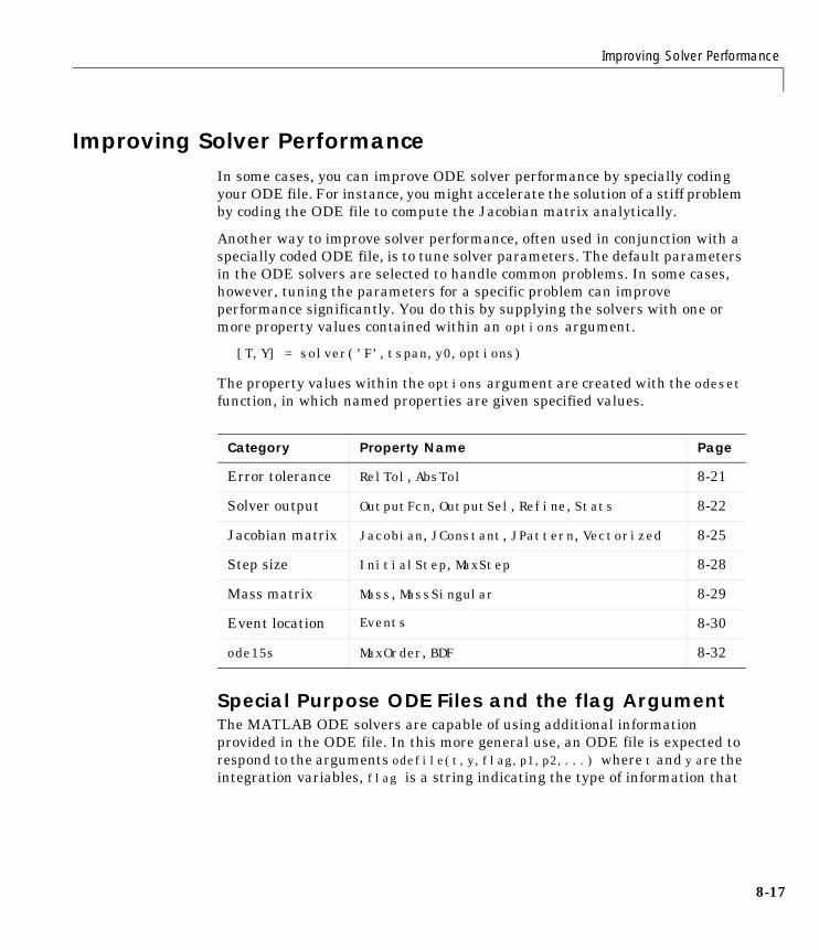
Another way to improve solver performance, often used in conjunction with a specially coded ODE file, is to tune solver parameters. The default parameters in the ODE solvers are selected to handle common problems. In some cases, however, tuning the parameters for a specific problem can improve performance significantly. You do this by supplying the solvers with one or more property values contained within an options argument.
[T,Y] = solver(’F’,tspan,y0,options)
The property values within the options argument are created with the odeset function, in which named properties are given specified values.
Special Purpose ODE Files and the flag ArgumentThe MATLAB ODE solvers are capable of using additional information provided in the ODE file. In this more general use, an ODE file is expected to respond to the arguments odefile(t,y,flag,p1,p2,...) where t and y are the integration variables, flag is a string indicating the type of information that
Category Property Name Page
Error tolerance RelTol, AbsTol 8-21
Solver output OutputFcn, OutputSel, Refine, Stats 8-22
Jacobian matrix Jacobian, JConstant, JPattern, Vectorized 8-25
Step size InitialStep, MaxStep 8-28
Mass matrix Mass, MassSingular 8-29
Event location Events 8-30
ode15s MaxOrder, BDF 8-32
8-17
8 Ordinary Differential Equations
8-1
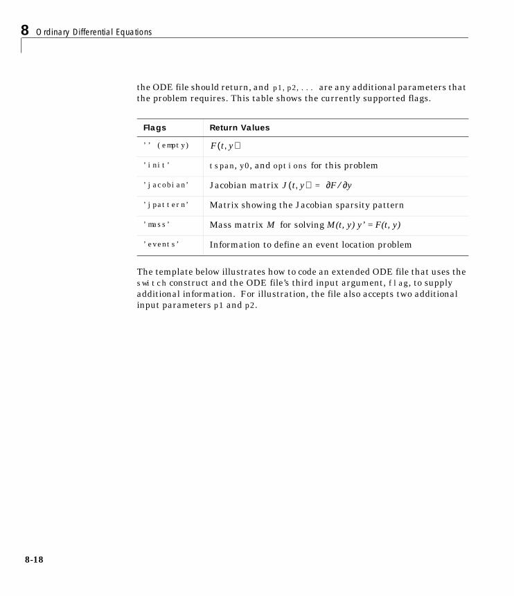
the ODE file should return, and p1,p2,... are any additional parameters that the problem requires. This table shows the currently supported flags.
The template below illustrates how to code an extended ODE file that uses the switch construct and the ODE file’s third input argument, flag, to supply additional information. For illustration, the file also accepts two additional input parameters p1 and p2.
Flags Return Values
’’ (empty)
’init’ tspan, y0, and options for this problem
’jacobian’ Jacobian matrix =
’jpattern’ Matrix showing the Jacobian sparsity pattern
’mass’ Mass matrix for solving M(t, y) y’ = F(t, y)
’events’ Information to define an event location problem
F t y,( )
J t y,( ) F∂ y∂⁄
M
8
Improving Solver Performance
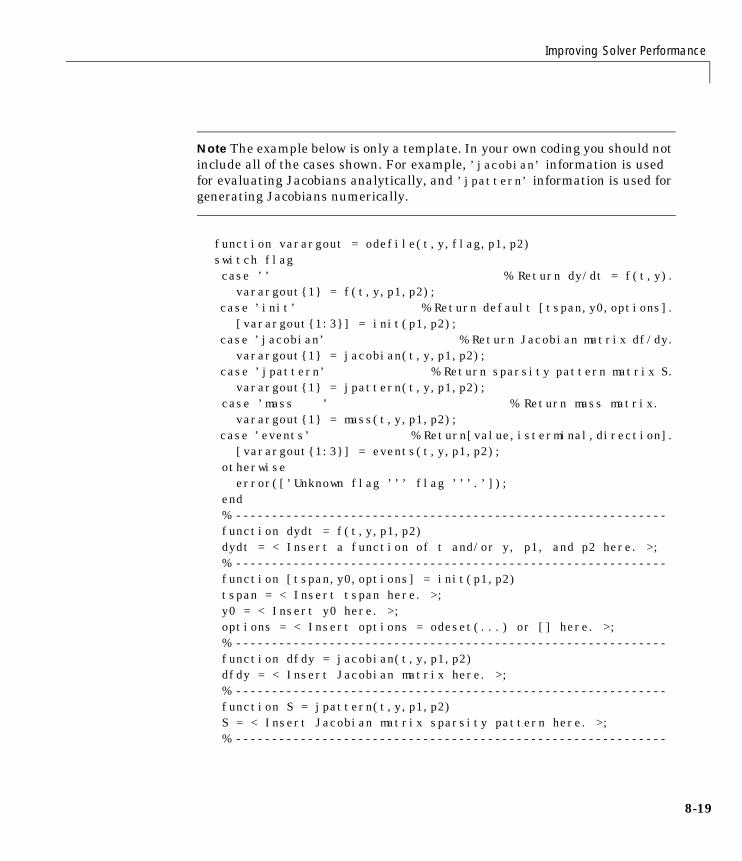
Note The example below is only a template. In your own coding you should not include all of the cases shown. For example, ’jacobian’ information is used for evaluating Jacobians analytically, and ’jpattern’ information is used for generating Jacobians numerically.
function varargout = odefile(t,y,flag,p1,p2)switch flag case ’’ % Return dy/dt = f(t,y). varargout{1} = f(t,y,p1,p2); case ’init’ % Return default [tspan,y0,options]. [varargout{1:3}] = init(p1,p2); case ’jacobian’ % Return Jacobian matrix df/dy. varargout{1} = jacobian(t,y,p1,p2); case ’jpattern’ % Return sparsity pattern matrix S. varargout{1} = jpattern(t,y,p1,p2); case ’mass ’ % Return mass matrix. varargout{1} = mass(t,y,p1,p2); case ’events’ % Return[value,isterminal,direction]. [varargout{1:3}] = events(t,y,p1,p2); otherwise error([’Unknown flag ’’’ flag ’’’.’]); end % ------------------------------------------------------------ function dydt = f(t,y,p1,p2) dydt = < Insert a function of t and/or y, p1, and p2 here. >; % ------------------------------------------------------------ function [tspan,y0,options] = init(p1,p2) tspan = < Insert tspan here. >; y0 = < Insert y0 here. >; options = < Insert options = odeset(...) or [] here. >; % ------------------------------------------------------------ function dfdy = jacobian(t,y,p1,p2) dfdy = < Insert Jacobian matrix here. >; % ------------------------------------------------------------ function S = jpattern(t,y,p1,p2) S = < Insert Jacobian matrix sparsity pattern here. >; % ------------------------------------------------------------
8-19
8 Ordinary Differential Equations
8-2
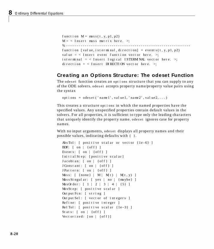
function M = mass(t,y,p1,p2)M = < Insert mass matrix here. >;% ------------------------------------------------------------function [value,isterminal,direction] = events(t,y,p1,p2)value = < Insert event function vector here. >;isterminal = < Insert logical ISTERMINAL vector here. >;direction = < Insert DIRECTION vector here. >;
Creating an Options Structure: The odeset FunctionThe odeset function creates an options structure that you can supply to any of the ODE solvers. odeset accepts property name/property value pairs using the syntax
options = odeset(’name1’,value1,’name2’,value2,...)
This creates a structure options in which the named properties have the specified values. Any unspecified properties contain default values in the solvers. For all properties, it is sufficient to type only the leading characters that uniquely identify the property name. odeset ignores case for property names.
With no input arguments, odeset displays all property names and their possible values, indicating defaults with { }.
AbsTol: [ positive scalar or vector {1e–6} ]BDF: [ on | {off} ]Events: [ on | {off} ]InitialStep: [positive scalar]Jacobian: [ on | {off} ]JConstant: [ on | {off} ]JPattern: [ on | {off} ]Mass: [ {none} | M | M(t) | M(t,y) ]MassSingular: [ yes | no | {maybe} ]MaxOrder: [ 1 | 2 | 3 | 4 | {5} ]MaxStep: [ positive scalar ]OutputFcn: [ string ]OutputSel: [ vector of integers ]Refine: [ positive integer ]RelTol: [ positive scalar {1e–3} ]Stats: [ on | {off} ]Vectorized: [on | {off}]
0
Improving Solver Performance
Modifying an Existing Options StructureTo modify an existing options argument, use
options = odeset(oldopts,’name1’,value1,...)
This sets options equal to the existing structure oldopts, overwriting any values in oldopts that are respecified using name/value pairs and adding to the structure any new pairs. The modified structure is returned as an output argument. In the same way, the command
options = odeset(oldopts,newopts)
combines the structures oldopts and newopts. In the output argument, any values in the second argument (other than the empty matrix) overwrite those in the first argument.
Querying Options: The odeget FunctionThe solvers use the odeget function to extract property values from an options structure created with odeset.
o = odeget(options,’name’)
This returns the value of the specified property, or an empty matrix [] if the property value is unspecified in the options structure.
As with odeset, it is sufficient to type only the leading characters that uniquely identify the property name; case is ignored for property names.
Error Tolerance PropertiesThe solvers use standard local error control techniques for monitoring and controlling the error of each integration step. At each step, the local error e in the i’th component of the solution is estimated and is required to be less than or equal to the acceptable error, which is a function of two user-defined tolerances RelTol and AbsTol.
|e(i)| <= max(RelTol*abs(y(i)),AbsTol(i))
• RelTol is the relative accuracy tolerance, a measure of the error relative to the size of each solution component. Roughly, it controls the number of correct digits in the answer. The default, 1e–3, corresponds to 0.1% accuracy.
8-21
8 Ordinary Differential Equations
8-2
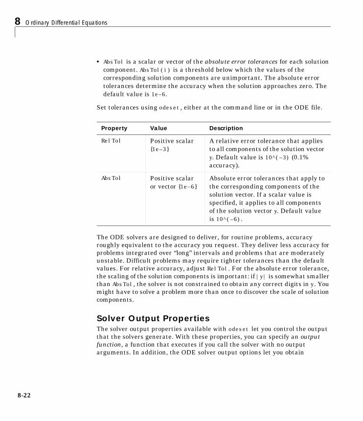
• AbsTol is a scalar or vector of the absolute error tolerances for each solution component. AbsTol(i) is a threshold below which the values of the corresponding solution components are unimportant. The absolute error tolerances determine the accuracy when the solution approaches zero. The default value is 1e–6.
Set tolerances using odeset, either at the command line or in the ODE file.
The ODE solvers are designed to deliver, for routine problems, accuracy roughly equivalent to the accuracy you request. They deliver less accuracy for problems integrated over “long” intervals and problems that are moderately unstable. Difficult problems may require tighter tolerances than the default values. For relative accuracy, adjust RelTol. For the absolute error tolerance, the scaling of the solution components is important: if |y| is somewhat smaller than AbsTol, the solver is not constrained to obtain any correct digits in y. You might have to solve a problem more than once to discover the scale of solution components.
Solver Output PropertiesThe solver output properties available with odeset let you control the output that the solvers generate. With these properties, you can specify an output function, a function that executes if you call the solver with no output arguments. In addition, the ODE solver output options let you obtain
Property Value Description
RelTol Positive scalar {1e–3}
A relative error tolerance that applies to all components of the solution vector y. Default value is 10^(–3) (0.1% accuracy).
AbsTol Positive scalar or vector {1e–6}
Absolute error tolerances that apply to the corresponding components of the solution vector. If a scalar value is specified, it applies to all components of the solution vector y. Default value is 10^(–6).
2
Improving Solver Performance
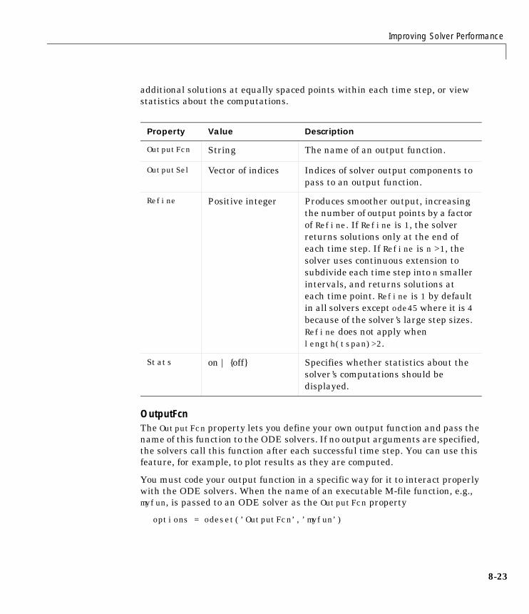
additional solutions at equally spaced points within each time step, or view statistics about the computations.
OutputFcn The OutputFcn property lets you define your own output function and pass the name of this function to the ODE solvers. If no output arguments are specified, the solvers call this function after each successful time step. You can use this feature, for example, to plot results as they are computed.
You must code your output function in a specific way for it to interact properly with the ODE solvers. When the name of an executable M-file function, e.g., myfun, is passed to an ODE solver as the OutputFcn property
options = odeset(’OutputFcn’,’myfun’)
Property Value Description
OutputFcn String The name of an output function.
OutputSel Vector of indices Indices of solver output components to pass to an output function.
Refine Positive integer Produces smoother output, increasing the number of output points by a factor of Refine. If Refine is 1, the solver returns solutions only at the end of each time step. If Refine is n >1, the solver uses continuous extension to subdivide each time step into n smaller intervals, and returns solutions at each time point. Refine is 1 by default in all solvers except ode45 where it is 4 because of the solver’s large step sizes. Refine does not apply when length(tspan)>2.
Stats on | {off} Specifies whether statistics about the solver’s computations should be displayed.
8-23
8 Ordinary Differential Equations
8-2
the solver calls it with myfun(tspan,y0,’init’) before beginning the integration so that the output function can initialize. Subsequently, the solver calls status = myfun(t,y) after each step. In addition to your intended use of (t,y), code myfun so that it returns a status output value of 0 or 1. If status = 1, integration halts. This might be used, for instance, to implement a STOP button. When integration is complete, the solver calls the output function with myfun([],[],’done’).
Some example output functions are included with the ODE solvers:
• odeplot – time series plotting
• odephas2 – two-dimensional phase plane plotting
• odephas3 – three-dimensional phase plane plotting
• odeprint – print solution as it is computed
Use these as models for your own output functions. odeplot is the default output function for all the solvers. It is automatically invoked when the solvers are called with no output arguments.
OutputSel The OutputSel property is a vector of indices specifying which components of the solution vector are to be passed to the output function. For example, if you want to use the odeplot output function, but you want to plot only the first and third components of the solution, you can do this using
options = odeset(’OutputFcn’,’odeplot’,’OutputSel’,[1 3]);
Refine The Refine property, an integer n, produces smoother output by increasing the number of output points by a factor of n. This feature is especially useful when using a medium or high order solver, such as ode45, for which solution components can change substantially in the course of a single step. To obtain smoother plots, increase the Refine property.
Note In all the solvers, the default value of Refine is 1.Within ode45, however, Refine is 4 to compensate for the solver’s large step sizes. To override this and see only the time steps chosen by ode45, set Refine to 1.
4
Improving Solver Performance
The extra values produced for Refine are computed by means of continuous extension formulas. These are specialized formulas used by the ODE solvers to obtain accurate solutions between computed time steps without significant increase in computation time.
Stats The Stats property specifies whether statistics about the computational cost of the integration should be displayed. By default, Stats is off. If it is on, after solving the problem the integrator displays:
• The number of successful steps
• The number of failed attempts
• The number of times the ODE file was called to evaluate F(t,y)
• The number of times that the partial derivatives matrix was formed
• The number of LU decompositions
• The number of solutions of linear systems
You can obtain the same values by including a third output argument in the call to the ODE solver:
[T,Y,S] = ode45(’myfun’, ...);
This statement produces a vector S that contains these statistics.
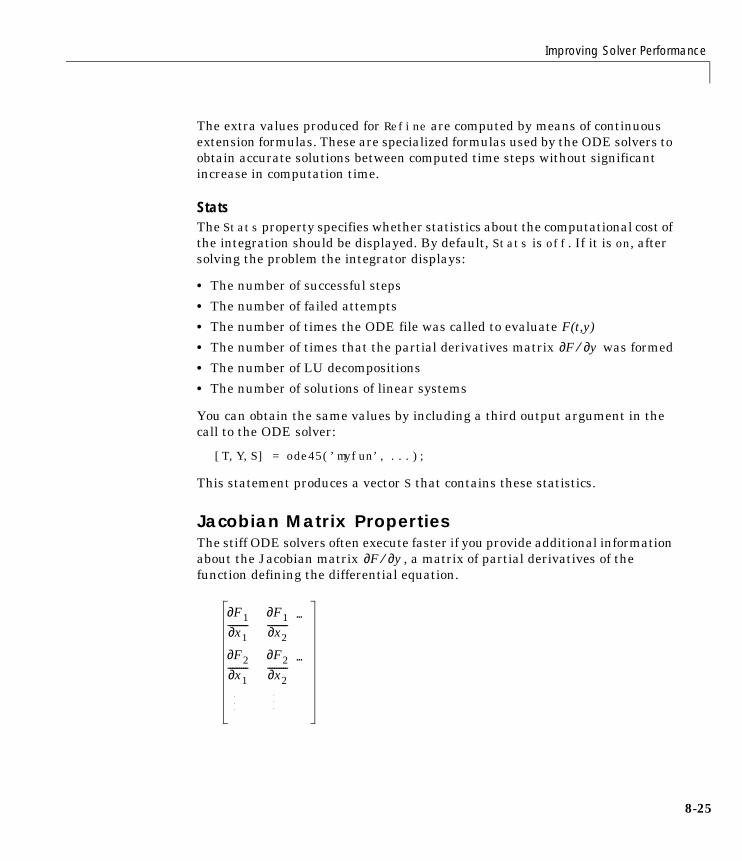
Jacobian Matrix PropertiesThe stiff ODE solvers often execute faster if you provide additional information about the Jacobian matrix , a matrix of partial derivatives of the function defining the differential equation.
F∂ y∂⁄
F∂ y∂⁄
F1∂x1∂---------
F1∂x2∂---------
···
F2∂x1∂---------
F2∂x2∂---------
···
.
.
.
.
.
.
8-25
8 Ordinary Differential Equations
8-2
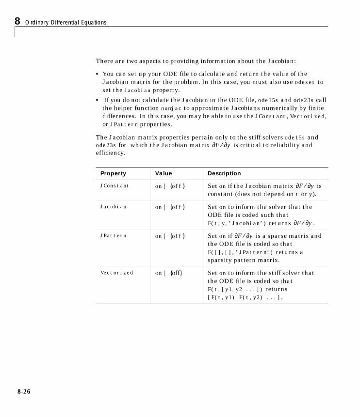
There are two aspects to providing information about the Jacobian:
• You can set up your ODE file to calculate and return the value of the Jacobian matrix for the problem. In this case, you must also use odeset to set the Jacobian property.
• If you do not calculate the Jacobian in the ODE file, ode15s and ode23s call the helper function numjac to approximate Jacobians numerically by finite differences. In this case, you may be able to use the JConstant, Vectorized, or JPattern properties.
The Jacobian matrix properties pertain only to the stiff solvers ode15s and ode23s for which the Jacobian matrix is critical to reliability and efficiency.
Property Value Description
JConstant on | {off} Set on if the Jacobian matrix is constant (does not depend on t or y).
Jacobian on | {off} Set on to inform the solver that the ODE file is coded such that F(t,y,’Jacobian’) returns .
JPattern on | {off} Set on if is a sparse matrix and the ODE file is coded so that F([],[],’JPattern’) returns a sparsity pattern matrix.
Vectorized on | {off} Set on to inform the stiff solver that the ODE file is coded so that F(t,[y1 y2 ...]) returns [F(t,y1) F(t,y2) ...].
F∂ y∂⁄
F∂ y∂⁄
F∂ y∂⁄
F∂ y∂⁄
6
Improving Solver Performance
JConstant Set JConstant on if the Jacobian matrix is constant (does not depend on t or y). Whether computing the Jacobians numerically or evaluating them analytically, the solver takes advantage of this information to reduce solution time. For the stiff van der Pol example, the Jacobian matrix is
J = [ 0 1 (–2000*y(1)*y(2) – 1) (1000*(1–y(1)^2)) ]
(not constant) so the JConstant property does not apply.
Jacobian Set Jacobian on to inform the solver that the ODE file is coded such that F(t,y,'Jacobian') returns . By default, Jacobian is off, and Jacobians are generated numerically.
Coding the ODE file to evaluate the Jacobian analytically often increases the speed and reliability of the solution for the stiff problem. The Jacobian shown above for the stiff van der Pol problem can be coded into the ODE file as
function out1 = vdp1000(t,y,flag)if strcmp(flag,’’) % return dyout1 = [y(2); 1000*(1–y(1)^2)*y(2)–y(1)];
elseif strcmp(flag,'jacobian') % return Jout1 = [ 0 1
(–2000*y(1)*y(2) – 1) (1000*(1–y(1)^2)) ];end
JPattern Set JPattern on if is a sparse matrix and the ODE file is coded so that F([],[],'JPattern') returns a sparsity pattern matrix. This is a sparse matrix with 1s where there are nonzero entries in the Jacobian. numjac uses the sparsity pattern to generate a sparse Jacobian matrix numerically. If the Jacobian matrix is large (size greater than approximately 100-by-100) and sparse, this can accelerate execution greatly. For an example using the JPattern property, see the brussode example on 8-37.
F∂ y∂⁄
F∂ y∂⁄
F∂ y∂⁄
8-27
8 Ordinary Differential Equations
8-2
Vectorized Set Vectorized on to inform the stiff solver that the ODE file is coded so that F(t,[y1 y2 ...]) returns [F(t,y1) F(t,y2) ...]. When computing Jacobians numerically, the solver passes this information to the numjac routine. This allows numjac to reduce the number of function evaluations required to compute all the columns of the Jacobian matrix, and may reduce solution time significantly.
With MATLAB’s array notation, it is typically an easy matter to vectorize an ODE file. For example, the stiff van der Pol example shown previously can be vectorized by introducing colon notation into the subscripts and by using the array power (.^) and array multiplication (.*) operators.
function dy = vdp1000(t,y)dy = [y(2,:); 1000*(1–y(1,:).^2).*y(2,:)–y(1,:)];
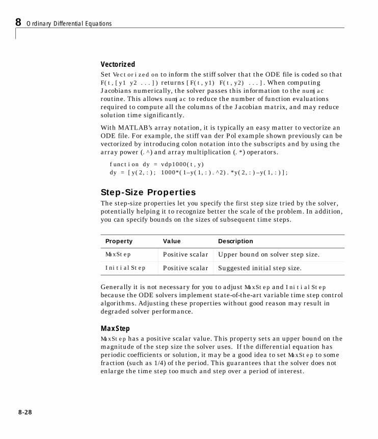
Step-Size PropertiesThe step-size properties let you specify the first step size tried by the solver, potentially helping it to recognize better the scale of the problem. In addition, you can specify bounds on the sizes of subsequent time steps.
Generally it is not necessary for you to adjust MaxStep and InitialStep because the ODE solvers implement state-of-the-art variable time step control algorithms. Adjusting these properties without good reason may result in degraded solver performance.
MaxStep MaxStep has a positive scalar value. This property sets an upper bound on the magnitude of the step size the solver uses. If the differential equation has periodic coefficients or solution, it may be a good idea to set MaxStep to some fraction (such as 1/4) of the period. This guarantees that the solver does not enlarge the time step too much and step over a period of interest.
Property Value Description
MaxStep Positive scalar Upper bound on solver step size.
InitialStep Positive scalar Suggested initial step size.
8
Improving Solver Performance
• Do not reduce MaxStep to produce more output points. This can slow down solution time significantly. Instead, use Refine (8-24) to compute additional outputs by continuous extension at very low cost.
• Do not reduce MaxStep when the solution does not appear to be accurate enough. Instead, reduce the relative error tolerance RelTol, and use the solution you just computed to determine appropriate values for the absolute error tolerance vector AbsTol. (See “Error Tolerance Properties” on page 8-21 for a description of the error tolerance properties.)
• Generally you should not reduce MaxStep to make sure that the solver doesn’t step over some behavior that occurs only once during the simulation interval. If you know the time at which the change occurs, break the simulation interval into two pieces and call the solvers twice. If you do not know the time at which the change occurs, try reducing the error tolerances RelTol and AbsTol. Use MaxStep as a last resort.
InitialStep InitialStep has a positive scalar value. This property sets an upper bound on the magnitude of the first step size the solver tries. Generally the automatic procedure works very well. However, the initial step size is based on the slope of the solution at the initial time tspan(1), and if the slope of all solution components is zero, the procedure might try a step size that is much too large. If you know this is happening or you want to be sure that the solver resolves important behavior at the start of the integration, help the code start by providing a suitable InitialStep.
Mass Matrix PropertiesThe solvers of the ODE suite can solve problems of the form M(t, y) y’ = F(t, y) with a mass matrix M that is nonsingular and (usually) sparse. Use odeset to set Mass to ’M’, ’M(t)’, or ’M(t,y)’ if the ODE file F.m is coded so that F(t,y,’mass’) returns a constant, time-dependent, or time-and-state dependent mass matrix, respectively. The default value of Mass is ’none’. The ode23s solver can only solve problems with a constant mass matrix M. For examples of mass matrix problems, see fem1ode, fem2ode, or batonode.
If M is singular, then M(t) * y’ = F(t, y) is a differential algebraic equation (DAE). DAEs have solutions only when y0 is consistent, that is, if there is a vector yp0 such that M(t0) * y0 = f(t0, y0). The ode15s and ode23t solvers can solve DAEs of index 1 provided that M is not state-dependent and y0 is
8-29
8 Ordinary Differential Equations
8-3
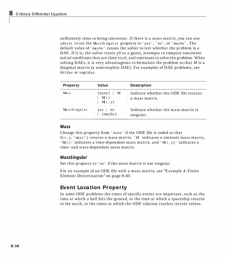
sufficiently close to being consistent. If there is a mass matrix, you can use odeset to set the MassSingular property to ’yes’, ’no’, or ’maybe’. The default value of ’maybe’ causes the solver to test whether the problem is a DAE. If it is, the solver treats y0 as a guess, attempts to compute consistent initial conditions that are close to y0, and continues to solve the problem. When solving DAEs, it is very advantageous to formulate the problem so that M is a diagonal matrix (a semi-explicit DAE). For examples of DAE problems, see hb1dae or amp1dae.
Mass Change this property from ’none’ if the ODE file is coded so that F(t,y,’mass’) returns a mass matrix. ’M’ indicates a constant mass matrix, ’M(t)’ indicates a time-dependent mass matrix, and ’M(t,y)’ indicates a time- and state-dependent mass matrix.
MassSingular Set this property to ’no’ if the mass matrix is not singular.
For an example of an ODE file with a mass matrix, see “Example 4: Finite Element Discretization” on page 8-40.
Event Location PropertyIn some ODE problems the times of specific events are important, such as the time at which a ball hits the ground, or the time at which a spaceship returns to the earth, or the times at which the ODE solution reaches certain values.
Property Value Description
Mass {none} | M | M(t) | M(t,y)
Indicate whether the ODE file returns a mass matrix.
MassSingular yes | no | {maybe}
Indicate whether the mass matrix is singular.
0
Improving Solver Performance
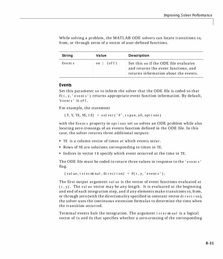
While solving a problem, the MATLAB ODE solvers can locate transitions to, from, or through zeros of a vector of user-defined functions.
Events Set this parameter on to inform the solver that the ODE file is coded so that F(t,y,’events’) returns appropriate event function information. By default, ’events’ is off.
For example, the statement
[T,Y,TE,YE,IE] = solver(’F’,tspan,y0,options)
with the Events property in options set on solves an ODE problem while also locating zero crossings of an events function defined in the ODE file. In this case, the solver returns three additional outputs:
• TE is a column vector of times at which events occur.
• Rows of YE are solutions corresponding to times in TE.
• Indices in vector IE specify which event occurred at the time in TE.
The ODE file must be coded to return three values in response to the ’events’ flag.
[value,isterminal,direction] = F(t,y,’events’);
The first output argument value is the vector of event functions evaluated at (t,y). The value vector may be any length. It is evaluated at the beginning and end of each integration step, and if any elements make transitions to, from, or through zero (with the directionality specified in constant vector direction), the solver uses the continuous extension formulas to determine the time when the transition occurred.
Terminal events halt the integration. The argument isterminal is a logical vector of 1s and 0s that specifies whether a zero-crossing of the corresponding
String Value Description
Events on | {off} Set this on if the ODE file evaluates and returns the event functions, and returns information about the events.
8-31
8 Ordinary Differential Equations
8-3
value element is terminal. 1 corresponds to a terminal event, halting the integration; 0 corresponds to a nonterminal event.
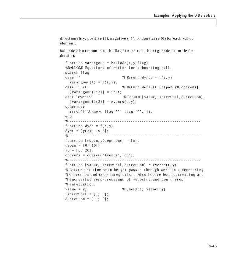
The direction vector specifies a desired directionality: positive (1), negative (–1), or don’t care (0), for each value element.
The time an event occurs is located to machine precision within an interval of [t– t+]. Nonterminal events are reported at t+. For terminal events, both t– and t+ are reported.
For an example of an ODE file with an event location, see “Example 5: Simple Event Location” on page 8-44.
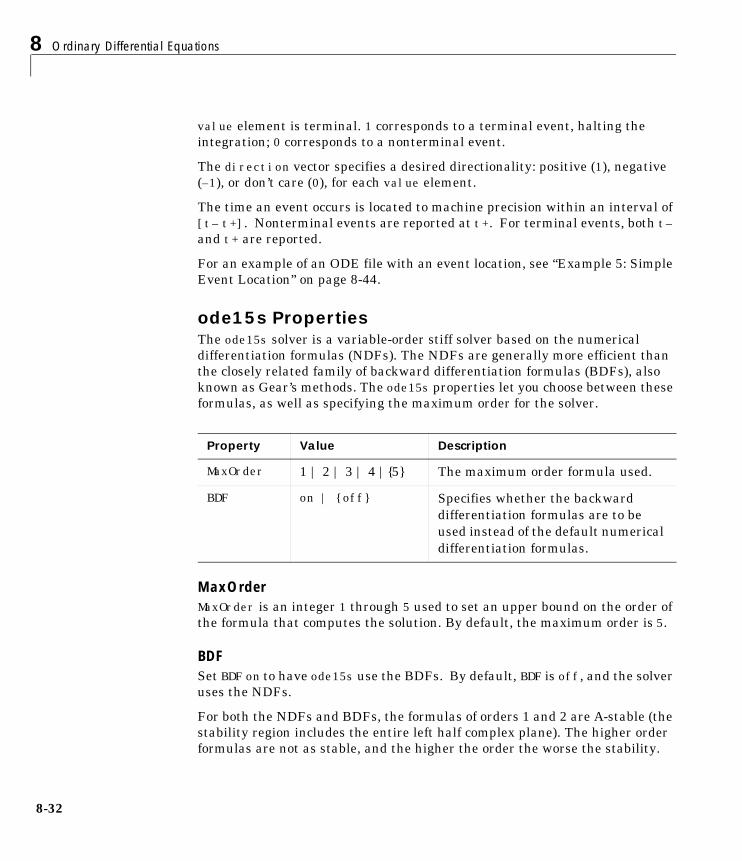
ode15s PropertiesThe ode15s solver is a variable-order stiff solver based on the numerical differentiation formulas (NDFs). The NDFs are generally more efficient than the closely related family of backward differentiation formulas (BDFs), also known as Gear’s methods. The ode15s properties let you choose between these formulas, as well as specifying the maximum order for the solver.
MaxOrderMaxOrder is an integer 1 through 5 used to set an upper bound on the order of the formula that computes the solution. By default, the maximum order is 5.
BDFSet BDF on to have ode15s use the BDFs. By default, BDF is off, and the solver uses the NDFs.
For both the NDFs and BDFs, the formulas of orders 1 and 2 are A-stable (the stability region includes the entire left half complex plane). The higher order formulas are not as stable, and the higher the order the worse the stability.
Property Value Description
MaxOrder 1 | 2 | 3 | 4 |{5} The maximum order formula used.
BDF on | {off} Specifies whether the backward differentiation formulas are to be used instead of the default numerical differentiation formulas.
2
Improving Solver Performance
There is a class of stiff problems (stiff oscillatory) that is solved more efficiently if MaxOrder is reduced (for example to 2) so that only the most stable formulas are used.
8-33
8 Ordinary Differential Equations
8-3
Examples: Applying the ODE SolversThis section contains several examples of ODE files. These examples illustrate the kinds of problems you can solve in MATLAB. For more examples, see MATLAB’s demos directory.
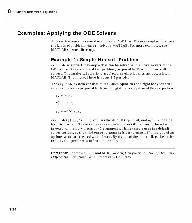
Example 1: Simple Nonstiff Problemrigidode is a nonstiff example that can be solved with all five solvers of the ODE suite. It is a standard test problem, proposed by Krogh, for nonstiff solvers. The analytical solutions are Jacobian elliptic functions accessible in MATLAB. The interval here is about 1.5 periods.
The rigidode system consists of the Euler equations of a rigid body without external forces as proposed by Krogh. rigidode is a system of three equations
rigidode([],[],’init’) returns the default tspan, y0, and options values for this problem. These values are retrieved by an ODE solver if the solver is invoked with empty tspan or y0 arguments. This example uses the default solver options, so the third output argument is set to empty, [], instead of an options structure created with odeset. By means of the ’init’ flag, the entire initial value problem is defined in one file.
Reference Shampine, L. F. and M. K. Gordon, Computer Solution of Ordinary Differential Equations, W.H. Freeman & Co., 1975.
y′3 0.51 y– 1 y2=
y′2 y– 1 y3=
y′1 y2 y3=
4
Examples: Applying the ODE Solvers
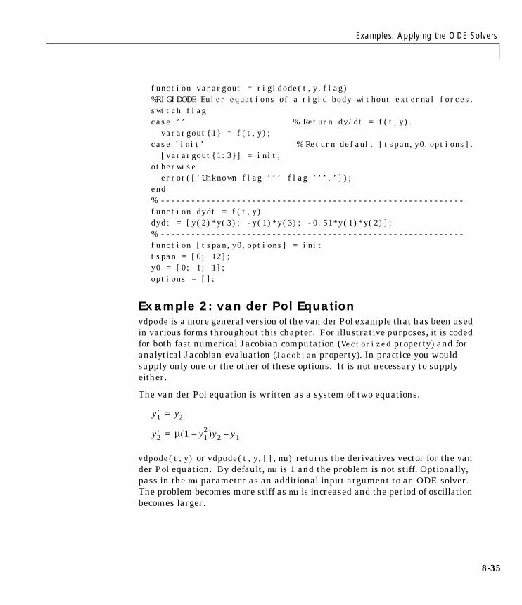
function varargout = rigidode(t,y,flag) %RIGIDODE Euler equations of a rigid body without external forces.switch flagcase ’’ % Return dy/dt = f(t,y). varargout{1} = f(t,y);case ’init’ % Return default [tspan,y0,options]. [varargout{1:3}] = init;otherwise error([’Unknown flag ’’’ flag ’’’.’]);end% ------------------------------------------------------------function dydt = f(t,y)dydt = [y(2)*y(3); -y(1)*y(3); -0.51*y(1)*y(2)];% ------------------------------------------------------------function [tspan,y0,options] = inittspan = [0; 12];y0 = [0; 1; 1];options = [];
Example 2: van der Pol Equation vdpode is a more general version of the van der Pol example that has been used in various forms throughout this chapter. For illustrative purposes, it is coded for both fast numerical Jacobian computation (Vectorized property) and for analytical Jacobian evaluation (Jacobian property). In practice you would supply only one or the other of these options. It is not necessary to supply either.
The van der Pol equation is written as a system of two equations.
vdpode(t,y) or vdpode(t,y,[],mu) returns the derivatives vector for the van der Pol equation. By default, mu is 1 and the problem is not stiff. Optionally, pass in the mu parameter as an additional input argument to an ODE solver. The problem becomes more stiff as mu is increased and the period of oscillation becomes larger.
y′2 µ(1 y12– )y2 y1–=
y′1 y2=
8-35
8 Ordinary Differential Equations
8-3
When mu is 1000 the equation is in relaxation oscillation and the problem is very stiff. The limit cycle has portions where the solution components change slowly and the problem is quite stiff, alternating with regions of very sharp change where it is not stiff (quasi-discontinuities).
This example sets Vectorized on with odeset because vdpode is coded so that vdpode(t,[y1 y2 ...]) returns [vdpode(t,y1) vdpode(t,y2) ...] for scalar time t and vectors y1,y2,... The stiff ODE solvers take advantage of this feature only when approximating the columns of the Jacobian numerically.
vdpode([],[],’init’) returns the default tspan, y0, and options values for this problem. The entire initial value problem is defined in this one file.
vdpode(t,y,’jacobian’) or vdpode(t,y,’jacobian’,mu) returns the Jacobian matrix evaluated analytically at (t,y). By default, the stiff solvers of the ODE suite approximate Jacobian matrices numerically. However, if Jacobian is set on with odeset, a solver calls the ODE file with the flag ’jacobian’ to obtain . Providing the solvers with an analytic Jacobian is not necessary, but it can improve the reliability and efficiency of integration.
F∂ y∂⁄
F∂ y∂⁄
6
Examples: Applying the ODE Solvers
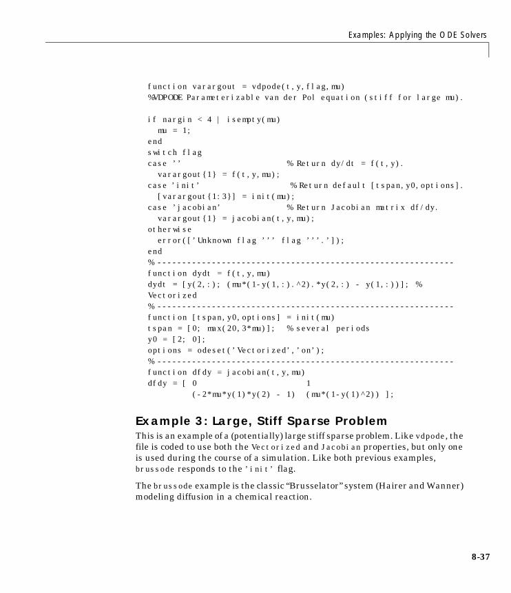
function varargout = vdpode(t,y,flag,mu)%VDPODE Parameterizable van der Pol equation (stiff for large mu).
if nargin < 4 | isempty(mu) mu = 1;endswitch flagcase ’’ % Return dy/dt = f(t,y). varargout{1} = f(t,y,mu);case ’init’ % Return default [tspan,y0,options]. [varargout{1:3}] = init(mu);case ’jacobian’ % Return Jacobian matrix df/dy. varargout{1} = jacobian(t,y,mu);otherwise error([’Unknown flag ’’’ flag ’’’.’]);end% ------------------------------------------------------------function dydt = f(t,y,mu)dydt = [y(2,:); (mu*(1-y(1,:).^2).*y(2,:) - y(1,:))]; % Vectorized% ------------------------------------------------------------function [tspan,y0,options] = init(mu)tspan = [0; max(20,3*mu)]; % several periodsy0 = [2; 0];options = odeset(’Vectorized’,’on’);% ------------------------------------------------------------function dfdy = jacobian(t,y,mu)dfdy = [ 0 1 (-2*mu*y(1)*y(2) - 1) (mu*(1-y(1)^2)) ];
Example 3: Large, Stiff Sparse ProblemThis is an example of a (potentially) large stiff sparse problem. Like vdpode, the file is coded to use both the Vectorized and Jacobian properties, but only one is used during the course of a simulation. Like both previous examples, brussode responds to the ’init’ flag.
The brussode example is the classic “Brusselator” system (Hairer and Wanner) modeling diffusion in a chemical reaction.
8-37
8 Ordinary Differential Equations
8-3
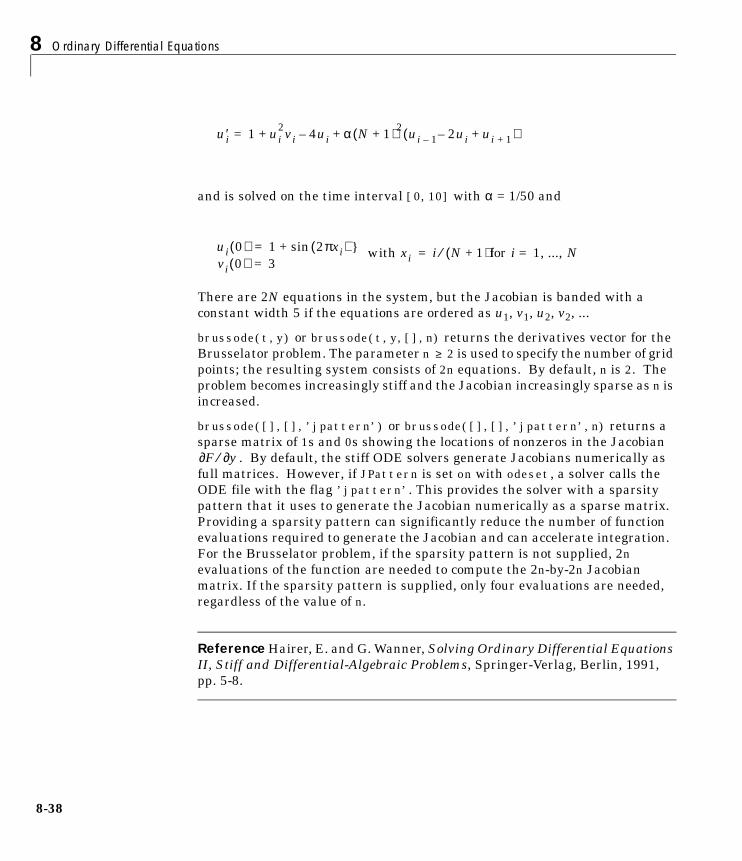
and is solved on the time interval [0,10] with α = 1/50 and
There are 2N equations in the system, but the Jacobian is banded with a constant width 5 if the equations are ordered as u1, v1, u2, v2, ...
brussode(t,y) or brussode(t,y,[],n) returns the derivatives vector for the Brusselator problem. The parameter n ≥ 2 is used to specify the number of grid points; the resulting system consists of 2n equations. By default, n is 2. The problem becomes increasingly stiff and the Jacobian increasingly sparse as n is increased.
brussode([],[],’jpattern’) or brussode([],[],’jpattern’,n) returns a sparse matrix of 1s and 0s showing the locations of nonzeros in the Jacobian
. By default, the stiff ODE solvers generate Jacobians numerically as full matrices. However, if JPattern is set on with odeset, a solver calls the ODE file with the flag ’jpattern’. This provides the solver with a sparsity pattern that it uses to generate the Jacobian numerically as a sparse matrix. Providing a sparsity pattern can significantly reduce the number of function evaluations required to generate the Jacobian and can accelerate integration. For the Brusselator problem, if the sparsity pattern is not supplied, 2n evaluations of the function are needed to compute the 2n-by-2n Jacobian matrix. If the sparsity pattern is supplied, only four evaluations are needed, regardless of the value of n.
Reference Hairer, E. and G. Wanner, Solving Ordinary Differential Equations II, Stiff and Differential-Algebraic Problems, Springer-Verlag, Berlin, 1991, pp. 5-8.
u′i 1 ui2vi 4ui– α N 1+( )2 ui 1– 2ui– ui 1++( )+ +=
ui 0( ) 1 2πxi( )vi 0( )
sin+3
==
with xi i N 1+( )⁄ for i 1, ..., N==}
F∂ y∂⁄
8
Examples: Applying the ODE Solvers
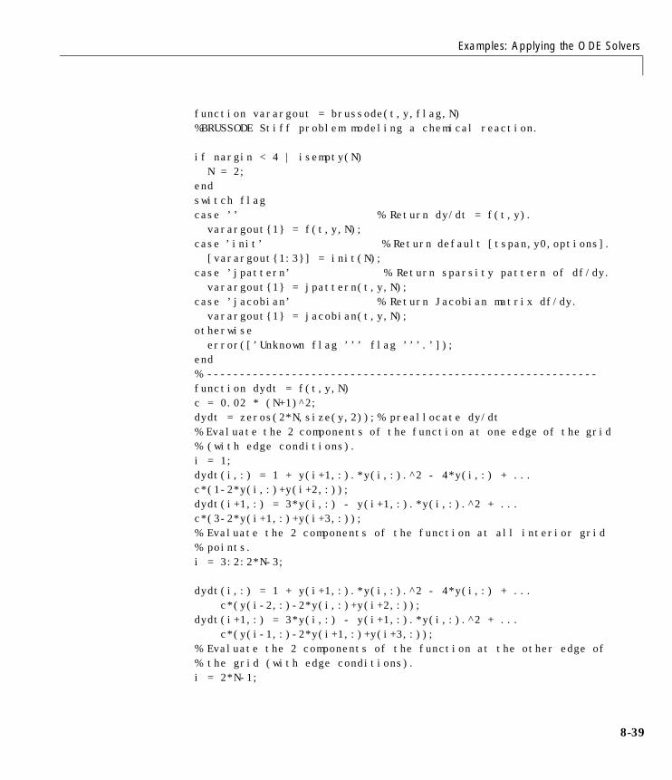
function varargout = brussode(t,y,flag,N)%BRUSSODE Stiff problem modeling a chemical reaction.
if nargin < 4 | isempty(N) N = 2;endswitch flagcase ’’ % Return dy/dt = f(t,y). varargout{1} = f(t,y,N);case ’init’ % Return default [tspan,y0,options]. [varargout{1:3}] = init(N);case ’jpattern’ % Return sparsity pattern of df/dy. varargout{1} = jpattern(t,y,N);case ’jacobian’ % Return Jacobian matrix df/dy. varargout{1} = jacobian(t,y,N);otherwise error([’Unknown flag ’’’ flag ’’’.’]);end% ------------------------------------------------------------function dydt = f(t,y,N)c = 0.02 * (N+1)^2;dydt = zeros(2*N,size(y,2));% preallocate dy/dt% Evaluate the 2 components of the function at one edge of the grid% (with edge conditions).i = 1;dydt(i,:) = 1 + y(i+1,:).*y(i,:).^2 - 4*y(i,:) + ... c*(1-2*y(i,:)+y(i+2,:));dydt(i+1,:) = 3*y(i,:) - y(i+1,:).*y(i,:).^2 + ... c*(3-2*y(i+1,:)+y(i+3,:));% Evaluate the 2 components of the function at all interior grid % points.i = 3:2:2*N-3;
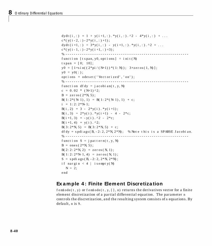
dydt(i,:) = 1 + y(i+1,:).*y(i,:).^2 - 4*y(i,:) + ... c*(y(i-2,:)-2*y(i,:)+y(i+2,:));dydt(i+1,:) = 3*y(i,:) - y(i+1,:).*y(i,:).^2 + ... c*(y(i-1,:)-2*y(i+1,:)+y(i+3,:));% Evaluate the 2 components of the function at the other edge of % the grid (with edge conditions).i = 2*N-1;
8-39
8 Ordinary Differential Equations
8-4
dydt(i,:) = 1 + y(i+1,:).*y(i,:).^2 - 4*y(i,:) + ... c*(y(i-2,:)-2*y(i,:)+1);dydt(i+1,:) = 3*y(i,:) - y(i+1,:).*y(i,:).^2 + ... c*(y(i-1,:)-2*y(i+1,:)+3);% ------------------------------------------------------------function [tspan,y0,options] = init(N)tspan = [0; 10];y0 = [1+sin((2*pi/(N+1))*(1:N)); 3+zeros(1,N)];y0 = y0(:);options = odeset(’Vectorized’,’on’);% ------------------------------------------------------------function dfdy = jacobian(t,y,N)c = 0.02 * (N+1)^2;B = zeros(2*N,5);B(1:2*(N-1),1) = B(1:2*(N-1),1) + c;i = 1:2:2*N-1;B(i,2) = 3 - 2*y(i).*y(i+1);B(i,3) = 2*y(i).*y(i+1) - 4 - 2*c;B(i+1,3) = -y(i).^2 - 2*c;B(i+1,4) = y(i).^2;B(3:2*N,5) = B(3:2*N,5) + c;dfdy = spdiags(B,-2:2,2*N,2*N); % Note this is a SPARSE Jacobian.% ------------------------------------------------------------function S = jpattern(t,y,N)B = ones(2*N,5);B(2:2:2*N,2) = zeros(N,1);B(1:2:2*N-1,4) = zeros(N,1);S = spdiags(B,-2:2,2*N,2*N);if nargin < 4 | isempty(N) N = 2;end
Example 4: Finite Element Discretization fem1ode(t,y) or fem1ode(t,y,[],n) returns the derivatives vector for a finite element discretization of a partial differential equation. The parameter n controls the discretization, and the resulting system consists of n equations. By default, n is 9.
0
Examples: Applying the ODE Solvers
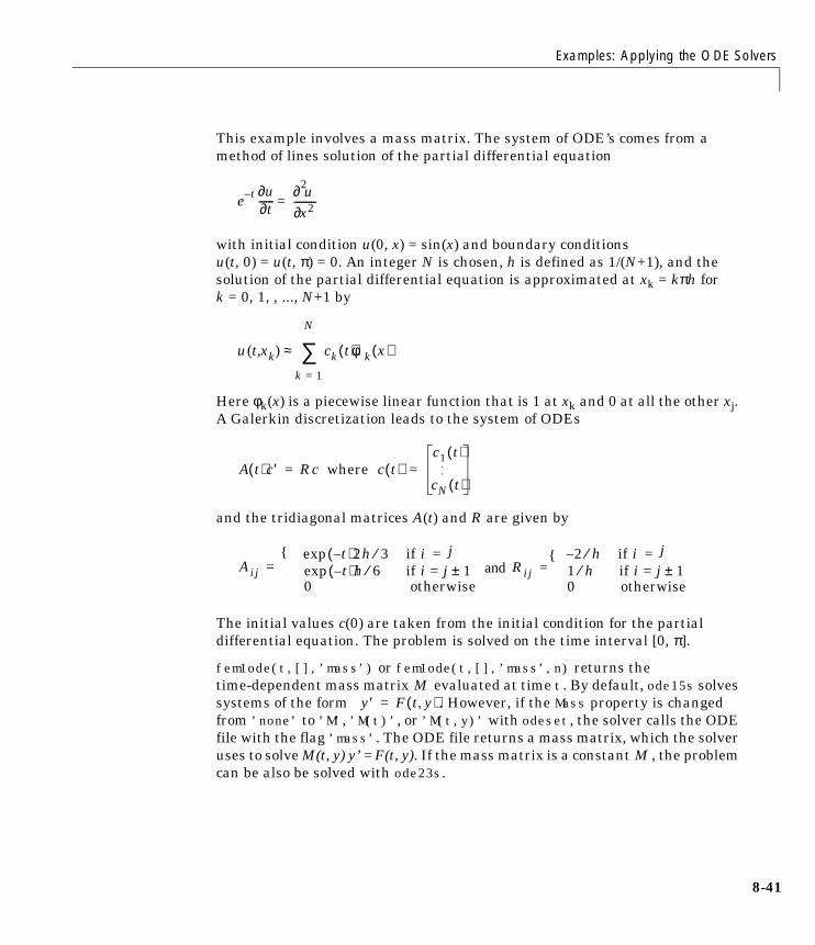
This example involves a mass matrix. The system of ODE’s comes from a method of lines solution of the partial differential equation
with initial condition u(0, x) = sin(x) and boundary conditions u(t, 0) = u(t, π) = 0. An integer N is chosen, h is defined as 1/(N+1), and the solution of the partial differential equation is approximated at xk = kπh fork = 0, 1, , ..., N+1 by
Here φk(x) is a piecewise linear function that is 1 at xk and 0 at all the other xj. A Galerkin discretization leads to the system of ODEs
and the tridiagonal matrices A(t) and R are given by
The initial values c(0) are taken from the initial condition for the partial differential equation. The problem is solved on the time interval [0, π].
fem1ode(t,[],’mass’) or fem1ode(t,[],’mass’,n) returns the time-dependent mass matrix evaluated at time t. By default, ode15s solves systems of the form . However, if the Mass property is changed from ’none’ to ’M’, ’M(t)’, or ’M(t,y)’ with odeset, the solver calls the ODE file with the flag ’mass’. The ODE file returns a mass matrix, which the solver uses to solve M(t, y) y’ = F(t, y). If the mass matrix is a constant , the problem can be also be solved with ode23s.
e t– u∂t∂------
∂2u∂x2---------=
u t xk( , ) ck t( )φk x( )
k 1=
N
∑≈
A t( )c′ Rc where c t( )c1 t( )
cN t( )= = .
.
exp t–( )2h 3⁄ if i jexp t–( )h 6⁄ if i j 10 otherwise
±=={
Aij = and2– h⁄ if i j
1 h⁄ if i j 10 otherwise
±==
Rij ={
My′ F t y,( )=
M
8-41
8 Ordinary Differential Equations
8-4
For example, to solve a system of 20 equations, use
[T,Y] = ode15s(’fem1ode’,[],[],odeset(’Mass’,’M(t)’),20);
2
Examples: Applying the ODE Solvers
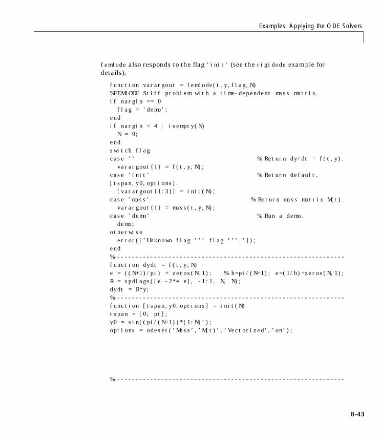
fem1ode also responds to the flag ’init’ (see the rigidode example for details).
function varargout = fem1ode(t,y,flag,N)%FEM1ODE Stiff problem with a time-dependent mass matrix.if nargin == 0 flag = ’demo’;endif nargin < 4 | isempty(N) N = 9;endswitch flagcase ’’ % Return dy/dt = f(t,y). varargout{1} = f(t,y,N);case ’init’ % Return default. [tspan,y0,options]. [varargout{1:3}] = init(N);case ’mass’ % Return mass matrix M(t). varargout{1} = mass(t,y,N);case ’demo’ % Run a demo. demo;otherwise error([’Unknown flag ’’’ flag ’’’.’]);end%---------------------------------------------------------------function dydt = f(t,y,N)e = ((N+1)/pi) + zeros(N,1); % h=pi/(N+1); e=(1/h)+zeros(N,1);R = spdiags([e -2*e e], -1:1, N, N);dydt = R*y;%---------------------------------------------------------------function [tspan,y0,options] = init(N)tspan = [0; pi];y0 = sin((pi/(N+1))*(1:N)’);options = odeset(’Mass’,’M(t)’,’Vectorized’,’on’);
%---------------------------------------------------------------
8-43
8 Ordinary Differential Equations
8-4
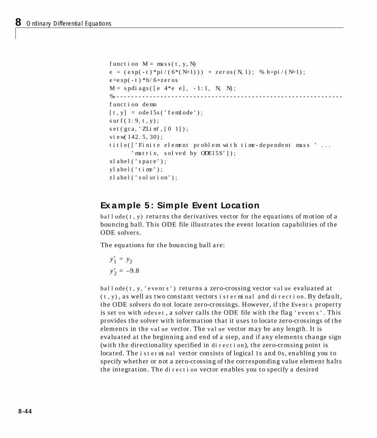
function M = mass(t,y,N)e = (exp(-t)*pi/(6*(N+1))) + zeros(N,1); % h=pi/(N+1); e=exp(-t)*h/6+zerosM = spdiags([e 4*e e], -1:1, N, N);%---------------------------------------------------------------function demo[t,y] = ode15s(’fem1ode’);surf(1:9,t,y);set(gca,’ZLim’,[0 1]);view(142.5,30);title([’Finite element problem with time-dependent mass ’ ... ’matrix, solved by ODE15S’]);xlabel(’space’);ylabel(’time’);zlabel(’solution’);
Example 5: Simple Event Locationballode(t,y) returns the derivatives vector for the equations of motion of a bouncing ball. This ODE file illustrates the event location capabilities of the ODE solvers.
The equations for the bouncing ball are:
ballode(t,y,’events’) returns a zero-crossing vector value evaluated at (t,y), as well as two constant vectors isterminal and direction. By default, the ODE solvers do not locate zero-crossings. However, if the Events property is set on with odeset, a solver calls the ODE file with the flag ’events’. This provides the solver with information that it uses to locate zero-crossings of the elements in the value vector. The value vector may be any length. It is evaluated at the beginning and end of a step, and if any elements change sign (with the directionality specified in direction), the zero-crossing point is located. The isterminal vector consists of logical 1s and 0s, enabling you to specify whether or not a zero-crossing of the corresponding value element halts the integration. The direction vector enables you to specify a desired
y′2 9.8–=
y′1 y2=
4
Examples: Applying the ODE Solvers
directionality, positive (1), negative (–1), or don’t care (0) for each value element.
ballode also responds to the flag ’init’ (see the rigidode example for details).
function varargout = ballode(t,y,flag)%BALLODE Equations of motion for a bouncing ball.switch flagcase ’’ % Return dy/dt = f(t,y). varargout{1} = f(t,y);case ’init’ % Return default [tspan,y0,options]. [varargout{1:3}] = init;case ’events’ % Return [value,isterminal,direction]. [varargout{1:3}] = events(t,y);otherwise error([’Unknown flag ’’’ flag ’’’.’]);end% ------------------------------------------------------------function dydt = f(t,y)dydt = [y(2); -9.8];% ------------------------------------------------------------function [tspan,y0,options] = inittspan = [0; 10];y0 = [0; 20];options = odeset(’Events’,’on’);% ------------------------------------------------------------function [value,isterminal,direction] = events(t,y)% Locate the time when height passes through zero in a decreasing % direction and stop integration. Also locate both decreasing and % increasing zero-crossings of velocity,and don’t stop % integration.value = y; % [height; velocity]isterminal = [1; 0];direction = [-1; 0];
8-45
8 Ordinary Differential Equations
8-4
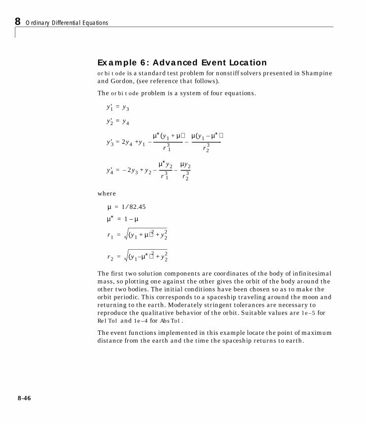
Example 6: Advanced Event Locationorbitode is a standard test problem for nonstiff solvers presented in Shampine and Gordon, (see reference that follows).
The orbitode problem is a system of four equations.
where
The first two solution components are coordinates of the body of infinitesimal mass, so plotting one against the other gives the orbit of the body around the other two bodies. The initial conditions have been chosen so as to make the orbit periodic. This corresponds to a spaceship traveling around the moon and returning to the earth. Moderately stringent tolerances are necessary to reproduce the qualitative behavior of the orbit. Suitable values are 1e–5 for RelTol and 1e–4 for AbsTol.
The event functions implemented in this example locate the point of maximum distance from the earth and the time the spaceship returns to earth.
y′2 y4=
y′1 y3=
y′3 2y4 y1
µ∗ y1 µ+( )
r31
---------------------------–µ y1 µ∗–( )
r23---------------------------–+=
y′4 2y3– y2
µ∗y2
r31
------------–µy2
r23---------–+=
µ 1 82.45⁄=
r2 y1 µ– ∗( )2 y22+=
r1 y1 µ+( )2 y22+=
µ∗ 1 µ–=
6
Examples: Applying the ODE Solvers
Reference Shampine, L. F. and M. K. Gordon, Computer Solution of Ordinary Differential Equations, W.H. Freeman & Co., 1975, p. 246.
8-47
8 Ordinary Differential Equations
8-4
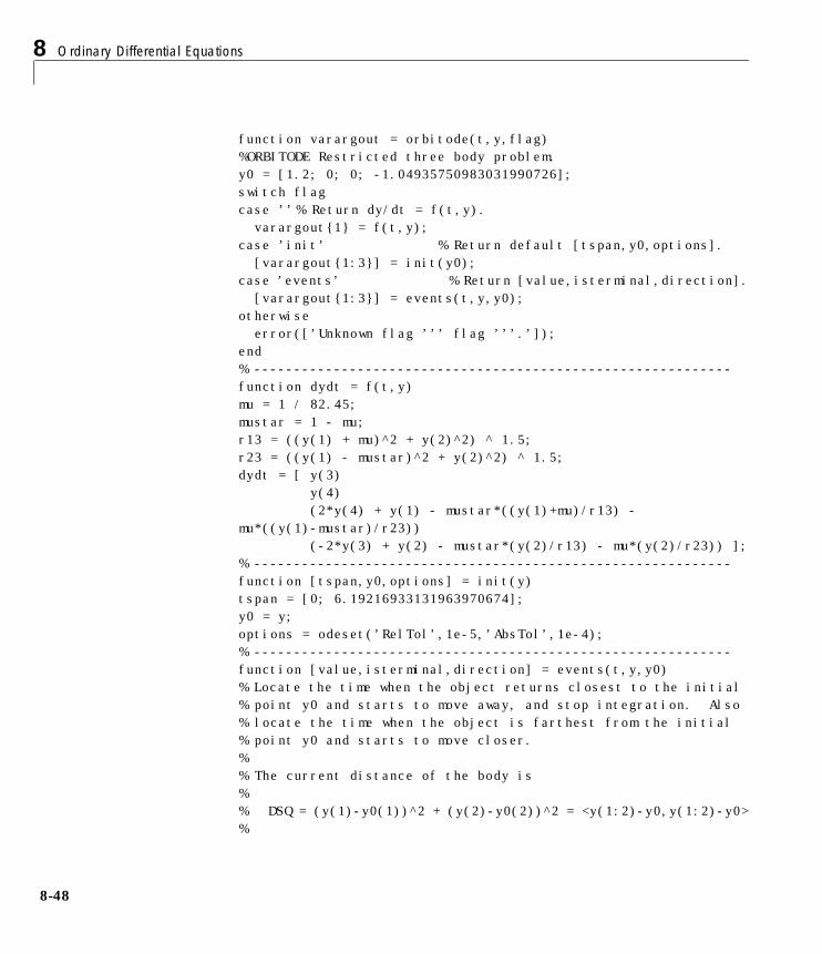
function varargout = orbitode(t,y,flag)%ORBITODE Restricted three body problem.y0 = [1.2; 0; 0; -1.04935750983031990726];switch flagcase ’’% Return dy/dt = f(t,y). varargout{1} = f(t,y);case ’init’ % Return default [tspan,y0,options]. [varargout{1:3}] = init(y0);case ’events’ % Return [value,isterminal,direction]. [varargout{1:3}] = events(t,y,y0);otherwise error([’Unknown flag ’’’ flag ’’’.’]);end% ------------------------------------------------------------function dydt = f(t,y)mu = 1 / 82.45;mustar = 1 - mu;r13 = ((y(1) + mu)^2 + y(2)^2) ^ 1.5;r23 = ((y(1) - mustar)^2 + y(2)^2) ^ 1.5;dydt = [ y(3) y(4) (2*y(4) + y(1) - mustar*((y(1)+mu)/r13) - mu*((y(1)-mustar)/r23)) (-2*y(3) + y(2) - mustar*(y(2)/r13) - mu*(y(2)/r23)) ];% ------------------------------------------------------------function [tspan,y0,options] = init(y)tspan = [0; 6.19216933131963970674];y0 = y;options = odeset(’RelTol’,1e-5,’AbsTol’,1e-4);% ------------------------------------------------------------function [value,isterminal,direction] = events(t,y,y0)% Locate the time when the object returns closest to the initial % point y0 and starts to move away, and stop integration. Also % locate the time when the object is farthest from the initial% point y0 and starts to move closer.% % The current distance of the body is% % DSQ = (y(1)-y0(1))^2 + (y(2)-y0(2))^2 = <y(1:2)-y0,y(1:2)-y0>%
8
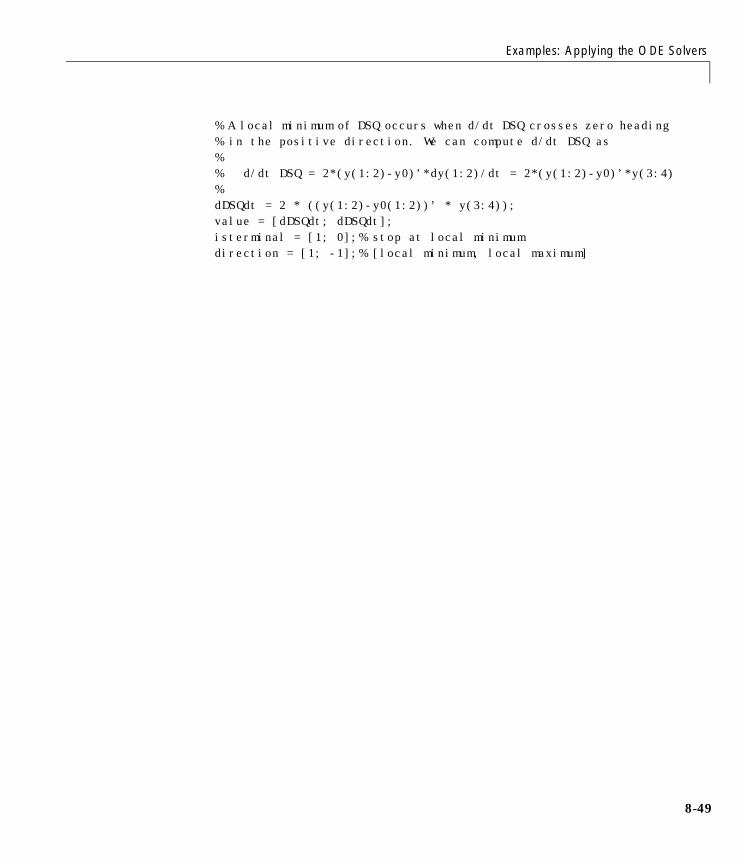
Examples: Applying the ODE Solvers
% A local minimum of DSQ occurs when d/dt DSQ crosses zero heading % in the positive direction. We can compute d/dt DSQ as% % d/dt DSQ = 2*(y(1:2)-y0)’*dy(1:2)/dt = 2*(y(1:2)-y0)’*y(3:4)% dDSQdt = 2 * ((y(1:2)-y0(1:2))’ * y(3:4));value = [dDSQdt; dDSQdt];isterminal = [1; 0];% stop at local minimumdirection = [1; -1];% [local minimum, local maximum]
8-49
8 Ordinary Differential Equations
8-5
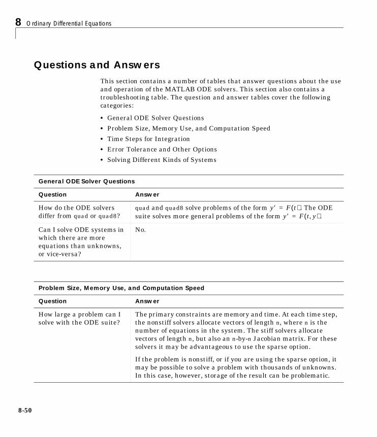
Questions and AnswersThis section contains a number of tables that answer questions about the use and operation of the MATLAB ODE solvers. This section also contains a troubleshooting table. The question and answer tables cover the following categories:
• General ODE Solver Questions
• Problem Size, Memory Use, and Computation Speed
• Time Steps for Integration
• Error Tolerance and Other Options
• Solving Different Kinds of Systems
General ODE Solver Questions
Question Answer
How do the ODE solvers differ from quad or quad8?
quad and quad8 solve problems of the form . The ODE suite solves more general problems of the form .
Can I solve ODE systems in which there are more equations than unknowns, or vice-versa?
No.
y′ F t( )=y′ F t y,( )=
Problem Size, Memory Use, and Computation Speed
Question Answer
How large a problem can I solve with the ODE suite?
The primary constraints are memory and time. At each time step, the nonstiff solvers allocate vectors of length n, where n is the number of equations in the system. The stiff solvers allocate vectors of length n, but also an n-by-n Jacobian matrix. For these solvers it may be advantageous to use the sparse option.
If the problem is nonstiff, or if you are using the sparse option, it may be possible to solve a problem with thousands of unknowns. In this case, however, storage of the result can be problematic.
0
Questions and Answers
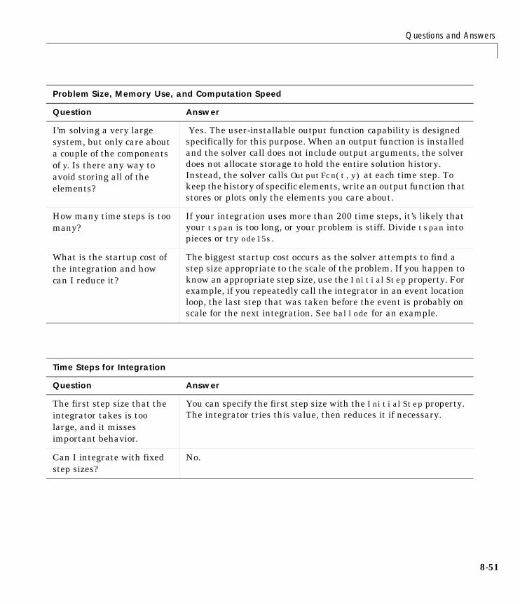
I’m solving a very large system, but only care about a couple of the components of y. Is there any way to avoid storing all of the elements?
Yes. The user-installable output function capability is designed specifically for this purpose. When an output function is installed and the solver call does not include output arguments, the solver does not allocate storage to hold the entire solution history. Instead, the solver calls OutputFcn(t,y) at each time step. To keep the history of specific elements, write an output function that stores or plots only the elements you care about.
How many time steps is too many?
If your integration uses more than 200 time steps, it’s likely that your tspan is too long, or your problem is stiff. Divide tspan into pieces or try ode15s.
What is the startup cost of the integration and how can I reduce it?
The biggest startup cost occurs as the solver attempts to find a step size appropriate to the scale of the problem. If you happen to know an appropriate step size, use the InitialStep property. For example, if you repeatedly call the integrator in an event location loop, the last step that was taken before the event is probably on scale for the next integration. See ballode for an example.
Problem Size, Memory Use, and Computation Speed
Question Answer
Time Steps for Integration
Question Answer
The first step size that the integrator takes is too large, and it misses important behavior.
You can specify the first step size with the InitialStep property. The integrator tries this value, then reduces it if necessary.
Can I integrate with fixed step sizes?
No.
8-51
8 Ordinary Differential Equations
8-5
Error Tolerance and Other Options
Question Answer
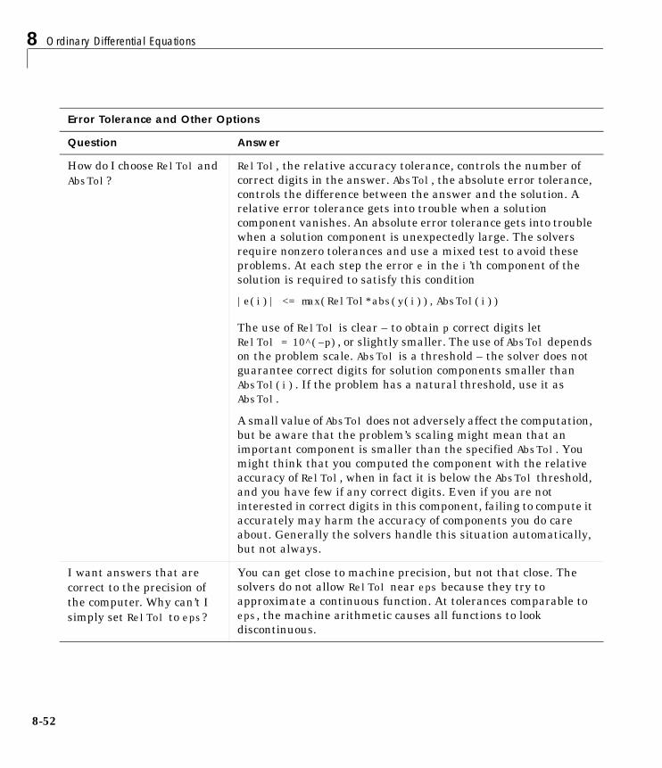
How do I choose RelTol and AbsTol?
RelTol, the relative accuracy tolerance, controls the number of correct digits in the answer. AbsTol, the absolute error tolerance, controls the difference between the answer and the solution. A relative error tolerance gets into trouble when a solution component vanishes. An absolute error tolerance gets into trouble when a solution component is unexpectedly large. The solvers require nonzero tolerances and use a mixed test to avoid these problems. At each step the error e in the i’th component of the solution is required to satisfy this condition
|e(i)| <= max(RelTol*abs(y(i)),AbsTol(i))
The use of RelTol is clear – to obtain p correct digits let RelTol = 10^(–p), or slightly smaller. The use of AbsTol depends on the problem scale. AbsTol is a threshold – the solver does not guarantee correct digits for solution components smaller than AbsTol(i). If the problem has a natural threshold, use it as AbsTol.
A small value of AbsTol does not adversely affect the computation, but be aware that the problem’s scaling might mean that an important component is smaller than the specified AbsTol. You might think that you computed the component with the relative accuracy of RelTol, when in fact it is below the AbsTol threshold, and you have few if any correct digits. Even if you are not interested in correct digits in this component, failing to compute it accurately may harm the accuracy of components you do care about. Generally the solvers handle this situation automatically, but not always.
I want answers that are correct to the precision of the computer. Why can’t I simply set RelTol to eps?
You can get close to machine precision, but not that close. The solvers do not allow RelTol near eps because they try to approximate a continuous function. At tolerances comparable to eps, the machine arithmetic causes all functions to look discontinuous.
2
Questions and Answers
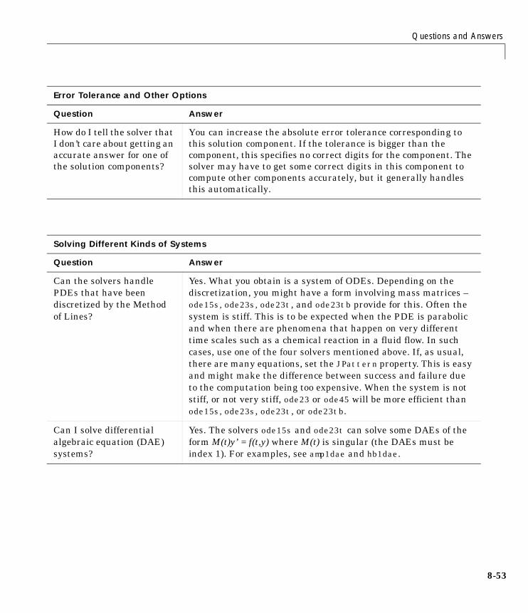
How do I tell the solver that I don’t care about getting an accurate answer for one of the solution components?
You can increase the absolute error tolerance corresponding to this solution component. If the tolerance is bigger than the component, this specifies no correct digits for the component. The solver may have to get some correct digits in this component to compute other components accurately, but it generally handles this automatically.
Error Tolerance and Other Options
Question Answer
Solving Different Kinds of Systems
Question Answer
Can the solvers handle PDEs that have been discretized by the Method of Lines?
Yes. What you obtain is a system of ODEs. Depending on the discretization, you might have a form involving mass matrices – ode15s, ode23s, ode23t, and ode23tb provide for this. Often the system is stiff. This is to be expected when the PDE is parabolic and when there are phenomena that happen on very different time scales such as a chemical reaction in a fluid flow. In such cases, use one of the four solvers mentioned above. If, as usual, there are many equations, set the JPattern property. This is easy and might make the difference between success and failure due to the computation being too expensive. When the system is not stiff, or not very stiff, ode23 or ode45 will be more efficient than ode15s, ode23s, ode23t, or ode23tb.
Can I solve differential algebraic equation (DAE) systems?
Yes. The solvers ode15s and ode23t can solve some DAEs of the form M(t)y’ = f(t,y) where M(t) is singular (the DAEs must be index 1). For examples, see amp1dae and hb1dae.
8-53
8 Ordinary Differential Equations
8-5
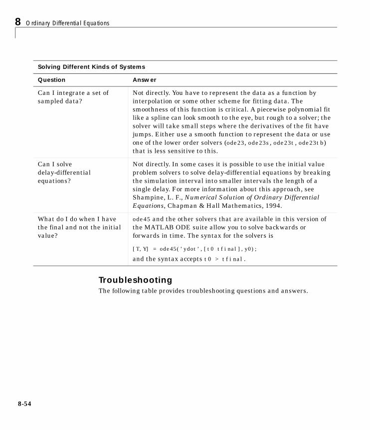
TroubleshootingThe following table provides troubleshooting questions and answers.
Can I integrate a set of sampled data?
Not directly. You have to represent the data as a function by interpolation or some other scheme for fitting data. The smoothness of this function is critical. A piecewise polynomial fit like a spline can look smooth to the eye, but rough to a solver; the solver will take small steps where the derivatives of the fit have jumps. Either use a smooth function to represent the data or use one of the lower order solvers (ode23, ode23s, ode23t, ode23tb) that is less sensitive to this.
Can I solve delay-differential equations?
Not directly. In some cases it is possible to use the initial value problem solvers to solve delay-differential equations by breaking the simulation interval into smaller intervals the length of a single delay. For more information about this approach, see Shampine, L. F., Numerical Solution of Ordinary Differential Equations, Chapman & Hall Mathematics, 1994.
What do I do when I have the final and not the initial value?
ode45 and the other solvers that are available in this version of the MATLAB ODE suite allow you to solve backwards or forwards in time. The syntax for the solvers is
[T,Y] = ode45(’ydot’,[t0 tfinal],y0);
and the syntax accepts t0 > tfinal.
Solving Different Kinds of Systems
Question Answer
4
Questions and Answers
Troubleshooting
Question Answer
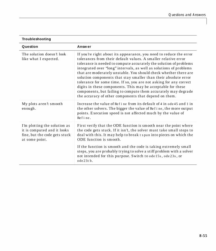
The solution doesn’t look like what I expected.
If you’re right about its appearance, you need to reduce the error tolerances from their default values. A smaller relative error tolerance is needed to compute accurately the solution of problems integrated over “long” intervals, as well as solutions of problems that are moderately unstable. You should check whether there are solution components that stay smaller than their absolute error tolerance for some time. If so, you are not asking for any correct digits in these components. This may be acceptable for these components, but failing to compute them accurately may degrade the accuracy of other components that depend on them.
My plots aren’t smooth enough.
Increase the value of Refine from its default of 4 in ode45 and 1 in the other solvers. The bigger the value of Refine, the more output points. Execution speed is not affected much by the value of Refine.
I’m plotting the solution as it is computed and it looks fine, but the code gets stuck at some point.
First verify that the ODE function is smooth near the point where the code gets stuck. If it isn’t, the solver must take small steps to deal with this. It may help to break tspan into pieces on which the ODE function is smooth.
If the function is smooth and the code is taking extremely small steps, you are probably trying to solve a stiff problem with a solver not intended for this purpose. Switch to ode15s, ode23s, or ode23tb.
8-55
8 Ordinary Differential Equations
8-5
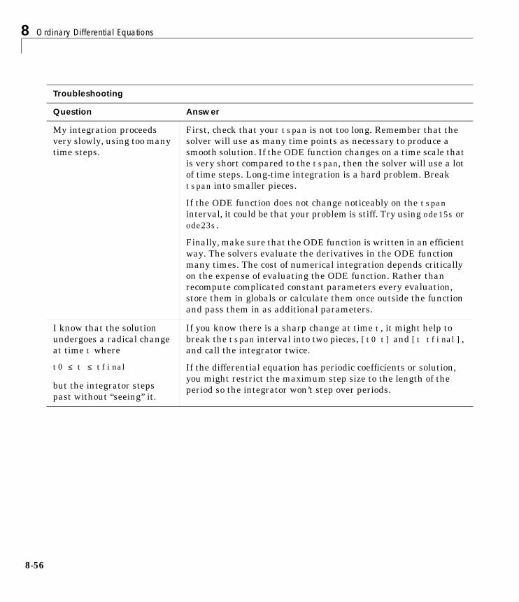
My integration proceeds very slowly, using too many time steps.
First, check that your tspan is not too long. Remember that the solver will use as many time points as necessary to produce a smooth solution. If the ODE function changes on a time scale that is very short compared to the tspan, then the solver will use a lot of time steps. Long-time integration is a hard problem. Break tspan into smaller pieces.
If the ODE function does not change noticeably on the tspan interval, it could be that your problem is stiff. Try using ode15s or ode23s.
Finally, make sure that the ODE function is written in an efficient way. The solvers evaluate the derivatives in the ODE function many times. The cost of numerical integration depends critically on the expense of evaluating the ODE function. Rather than recompute complicated constant parameters every evaluation, store them in globals or calculate them once outside the function and pass them in as additional parameters.
I know that the solution undergoes a radical change at time t where
t0 ≤ t ≤ tfinal
but the integrator steps past without “seeing” it.
If you know there is a sharp change at time t, it might help to break the tspan interval into two pieces, [t0 t] and [t tfinal], and call the integrator twice.
If the differential equation has periodic coefficients or solution, you might restrict the maximum step size to the length of the period so the integrator won’t step over periods.
Troubleshooting
Question Answer
6