first emptiness in queueing, storage, and traffic

FIRST EMPTINESS PROBLEMSIN QUEUEING, STORAGE,AND TRAFFIC THEORY

J. GANIMANCHESTER-SHEFFIELD

SCHOOL OF PROBABILITY AND STATISTICS

1. Introduction

One of the aims of the Berkeley Symposium is to encourage research workersto present a summary of results newly obtained in their fields during theprevious five years. In accordance with this intention, the earlier part of thepresent paper will describe some interesting developments in problems of firstemptiness since 1965. For simplicity, only first passage problems (to the zerostate) for certain discrete time random walks on the integers 0, 1, 2, * , will bediscussed. As is already known, first emptiness probabilities are of considerableimportance in queueing, storage, and traffic problems. Their distributions maybe interpreted

(a) in queueing theory, as probability distributions of the length of a busyperiod during which all waiting customers have been served, so that the queueis empty;

(b) in storage theory, as probability distributions of the times to first empti-ness of a reservoir, all the stored water having been released;

(c) in traffic theory, as probability distributions of periods to a first gap at a"give way" intersection on a minor road, all vehicles crossing the road havingpassed, so that the intersection becomes empty and through traffic on the roadcan proceed.A graphical representation of a random walk in discrete time of the type

which arises in queueing, storage, and traffic processes is provided in Figure 1.Here Z0 = u is the initial state of the random walk at time t = 0; this representsthe number of customers initially waiting for service in a queue, the units ofwater initially contained in a reservoir, or the number of vehicles initially waitingto cross a minor road, thus blocking the traffic along it.The sequence of discrete nonnegative random variables {X,},o'0 constitutes the

inputs into the system during the time intervals (t, t + 1), t = 0, 1, . At theend of each time interval, there is a unit output if the random walk lies in anyone of the states 1, 2, 3, . *, or a zero output if it is in state zero. Inputsrepresent new arrivals at a queue, new water inflows into a reservoir, or new

Research supported by the Office of Naval Research and the Federal Highway Administration.

515

516 SIXTH BERKELEY SYMPOSIUM: GANI

U -0 1X -- T,

0 I 2 3 4 5 T-3 T-2 T- T- t t+FIGURE 1

Random walk with first emptiness at T = T(u).

vehicles preparing to cross a minor road in traffic; outputs denote a servicedcustomer in queueing, a released unit of water from a reservoir, or a vehiclewhich has crossed the minor road in traffic. For such processes, the randomwalk {Z,}t - may be characterized by the relation

(1.1) Zt+1 = {Zt + X, - 1}+ t = 0O l, 2, *,where the positive index indicates the greater of Z, + X, - 1 and 0.The time to first emptiness of the process starting from ZO = u will be denoted

by T = T(u); it is clear that for t = 0O l,1 , T,

(1.2) Zt+ = Z, + Xt-l,with Zt becoming zero for the first time when t = T. Note that in Figure 1 wehave written Tj, j = 1. , u, for the first passage time of the random walk tostate u - j starting from state u + 1 - j, so that

U

(1.3) T(u) = T1 + T2 + + Tu =Z Tjj= ,

rhe first part of this paper will deal mainly with recent research on the propertiesof T(u) when the inputs {X,} form a Markov chain with a finite or denumerablyinfinite state space. We shall see that the newly derived results are similar tothose previously known for independently and identically distributed (i.i.d.)inputs.We shall also denote by Wj, j = 1, , u, the stochastic integral under the

first passage path leading from state u + - j to state u - j and lying above

FIRST EMPTINESS PROBLEMS 517

the line u-j (see Figure 1). The path integral WH corresponds to the firstpassage time Tj. Clearly, the stochastic integral W(u) lying under the path tofirst emptiness starting from state u is given by

(1.4) W(u) = {W1 + (u - 1)T1} + {W2 + (u - 2)T2} + + {W.}U

- E {Wi + (U-j)Tj}j=1

In the second part of the paper, we formulate some problems for stochastic pathintegrals of this type when the inputs {X,} are either i.i.d. or Markovian, andderive initial results for their probability distributions. Much remains to bedone in this area; it is hoped that research workers will be encouraged to attacksome of the many unsolved problems in the field.

2. Known results on first emptiness for i.i.d. inputs {X,}From Figure 1, it is intuitively obvious that if the inputs {X,} are i.i.d., the

random variables Tp, j = 1, , u, will also be i.i.d: It follows that the distri-bution of T(u) in (1.3) is the uth convolution of the distribution of Ti. This maybe demonstrated more formally as follows. Let

00(2.1) g(O; U) = E g(T; u)OT? 0 . 0 < 1,T=u

be the probability generating function (p.g.f.) for the first emptiness time T(u)of the random walk (1.1) with initial state ZO = u > 1, subject to i.i.d. inputs{X,}. It is readily shown that

(2.2) g(0; U) = {g(0; l)}U.Assume z to be the line of first descent of the random walk from state u to

state 1; then clearly, the first emptiness probability g(T; u) may be decomposedas

T-1

(2.3) g(T; u) = g(z; u - 1)g(T - z: 1).r=u-1

Forming the p.g.f. of this distribution, we obtain.o T-1

(2.4) g(0; U) = E 0T 1 g(z; u - l)g(T - z; 1)T=u r=u-1

= g(z: u - 1)0 g(T - z;r=u-1 T=r+ 1

= g(0: u - 1)g(0; 1).Continuing the reduction of g(0: u - 1), we readily find result (2.2); this wasoriginally derived in a somewhat different form by Kendall [13] in 1957.


Following (2.2), a second more interesting result, reminiscent of that holdingfor probabilities of first extinction in branching processes may be derived for thep.g.f. g(0; 1). Namely, if p(0) = = piO denotes the p.g.f. of any one of therandom variables X,, then g(O; 1) satisfies the functional equation

(2.5) g(6; 1) = Op(g(6; 1))subject to the condition g(O; 1) = 0. A proof of the equivalent result for a par-ticular continuous time process in queueing may be found in the basic 1955paper of Takdcs [24]; its derivation for the more general case was sketched byKendall [13] in 1957. The argument in discrete time may be given very simplyas follows. Let the input XO during the time interval (0, 1) in a random walkwith initial state ZO = 1 be i = 0, 1, 2, - - . If the input is zero, first emptinessoccurs at T = 1, but if i > 1, the first emptiness process will continue from timet = 1, starting now from Z1 = i. Thus, the p.g.f. g(O; 1) will be given by theequation

(2.6) g(0; 1) = Po0 + 0 E pig(o; i);

but from (2.2), we see that this may be rewritten as

(2.7) g(O; 1) = Po0 + 0 E pi{g(6; 1)}W= Op(g(O; 1))

leading to the result (2.5), where g(O; 1) = 0.Precisely as in branching process theory, it is easily shown that

g(l-; 1) = C = 1 if E(XJ) = p'(l) < 1,(2.8) g(l-; 1) = C < 1 if E(XJ) = p'(l) > 1.

Takics [24] first obtained the explicit form of g(T; 1) for Poisson inputs offixed size, and Kendall [13] later derived the general formula (but in continuoustime, from an integral equation) of type

(2.9) g(T; u) =- (T) = 1, 2, ,

where p(T) - Pr {X0 + X1 + * + XT.- 1 = T - u} for arbitrary i.i.d. inputdistributions. Perhaps the simplest analytic method of obtaining this result isfrom the functional equation (2.5), using Lagrange's method of reversion ofseries. It has also been derived in an elementary manner by Lloyd [15] in 1963,using difference equation methods. But (2.9) is perhaps best viewed com-binatorially as recording the proportion ulT of permissible paths leading toemptiness from among all those satisfying the condition XO + X1 + ... +

XTl1 = T -U.


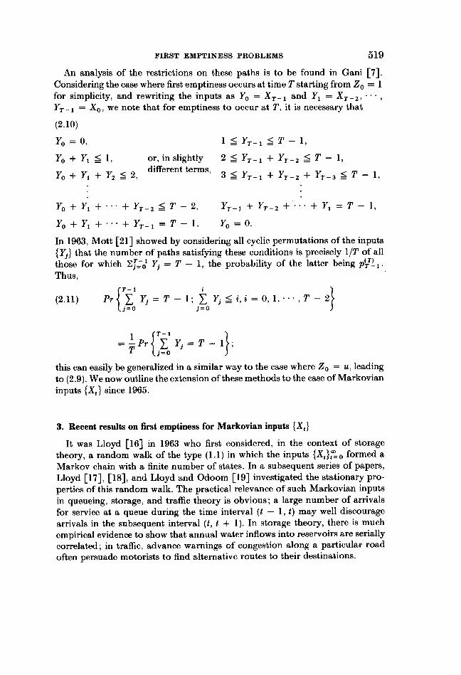
An analysis of the restrictions on these paths is to be found in Gani [7].Considering the case where first emptiness occurs at time T starting from Z0 = 1for simplicity, and rewriting the inputs as YO = XT-1 and Y1 = XT-2,'YT- 1 = X0, we note that for emptiness to occur at T, it is necessary that

(2.10)

YO = °, 1<l YT-1 -T- ,

Y0+ Y1 < 1, or, in slightly 2 -YT-1 + YT-2 < T -1,

YO + Y1 + Y2 . 2, different terms, 3 < YT-1 + YT-2 + YT-3 = T

YO+ Y1 + + YT-2 _ T - 2, YT-1 + YT-2 + + Y1 =T -1,

Yo+ Y1 + + YT-1 T-1, YO = 0.

In 1963, Mott [21] showed by considering all cyclic permutations of the inputs{Yj} that the number of paths satisfying these conditions is precisely 1/T of allthose for which EJT- 1 Yj = T -1, the probability of the latter being p(T)1.Thus,

T-1

j=0 j=o

TPr{ Yj = T -1

this can easily be generalized in a similar way to the case where Z0 = u, leadingto (2.9). We now outline the extension of these methods to the case of Markovianinputs {X,} since 1965.

3. Recent results on first emptiness for Markovian inputs {XJIt was Lloyd [16] in 1963 who first considered, in the context of storage

theory, a random walk of the type (1.1) in which the inputs {X,}t'=o formed aMarkov chain with a finite number of states. In a subsequent series of papers,Lloyd [17], [18], and Lloyd and Odoom [19] investigated the stationary pro-perties of this random walk. The practical relevance of such Markovian inputsin queueing, storage, and traffic theory is obvious; a large number of arrivalsfor service at a queue during the time interval (t - 1, t) may well discouragearrivals in the subsequent interval (t, t + 1). In storage theory, there is muchempirical evidence to show that annual water inflows into reservoirs are seriallycorrelated; in traffic, advance warnings of congestion along a particular roadoften persuade motorists to find alternative routes to their destinations.


For convenience we shall assume, unless it is stated otherwise, that the inputX_-1 in the interval (- 1, 0) before the process {Z,} begins is zero. For inputs{X,}'o forming an irreducible Markov chain with stationary transitionprobabilities

(3.1) Pij = Pr {X,+, = j|X, = i}, i,j = 0, 1, , r,

it is known that the Tjj = 1, * , u, in Figure 1 are once again i.i.d. (seeChung [4]). It follows as before that the distribution of T(u) in (1.3) will be theuth convolution of the distribution of T1. As in the case of i.i.d. inputs, thismay be proved formally as follows. Let

(3.2) g(0; u,0) = E g(T; U,0)0T, 0 _ 0 < 1,T=u

be the p.g.f. of the first emptiness probabilities g(T; u, 0) = g(T; u, X 1 = 0)of T(u), subject to Markovian inputs {X,}. Again assuming r to be the time offirst descent to state 1, we may write

T-1

(3.3) g(T; u, 0) = E g(z; u - 1, 0)g(T - r; 1, 0).z=u-1

Forming the p.g.f. with respect to T we find, much as in (2.2) through (2.4),that

X T-1

(3.4) g(O; U, 0) = E ST E g(r; u - 1, 0)g(T - T; 1, 0)T=u T=u-1

= g(0; u - 1, 0)g(0; 1, 0) = {g(0; 1, 0)}".

For Markovian inputs, Ali Khan and Gani [1] showed in 1968 that g(0; 1, 0)satisfies a functional equation similar to (2.5), of the form

(3.5) g(0; 1, 0) = 0)(g(O; 1, 0))

subject to g'(0; 1, 0) = poo. Here A(0) is the simple maximum eigenvalue of thepositive matrix

Poo Po00 V020 ... POr0'

(3.6) {PijO}ij=o = P1o Pu10 P1202 ** Plr0 , 0 < 0 . 1,

[PrO Pr10 Pr202 .. PrroJsuch that A(1) = 1 and A(0) = poo, where all pij may be taken positive forsimplicity. This eigenvalue, though positive and strictly monotonic increasingfor 0 > 0, is not in general a p.g.f.; it is shown in Gani [8] that when expanded inpowers of 0, the generating function

- AW(Oi},(3.7) A(0) = 1 ()o0

i=o


may have negative coefficients 2(i)(0) for i . 2. When the {X,} are i.i.d. so thatpij = pj, equation (3.5) reduces to the better known functional relation (2.5).We now proceed to prove (3.5).

Following precisely the same approach as that leading to (2.6), we readilyfind for the random walk with Markovian inputs starting from ZO = 1 that

(3.8) g(0 1.0i) = pOo0 ± 0 E p0ig(0: i. i),

where

(3.9) g(f: i, i) = g(0: Z1 =. i X0 = i)

denotes the p.g.f. of first emptiness times starting from Z1 = i. with prior inputX0 = i instead of the usual zero. A decomposition similar to (3.4) yields

(3.10) g(0: i) = g(0: 1. i){g(0; 1, 0)}'1 i _1substituting this in (3.8). we are led directly to the relation

(3.11) g(O; 1.0) = 0 E poig(O; 1, i){g(0; 1, 0)}i 1.i=o

In exactly the same way, we may show that

(3.12) g(0: 1. k) = 0 E pkig(O: 1, i){g(O: 1. 0)}i-. k = 1, . r.i=o

Hence, multiplying both (3.11) and (3.12) by g(O; 1, 0) and setting out theresults in matrix form, we obtain

g(O);I0) OPoo p01g POr'gr g(O; 1, 0)

( g(0 1 1) P p11g ... p gr g(O: 1.I)

( g(O:1. r) 1=0 KP;g ...Prrg_jg(O:1.r)where g = g(O; 1, 0) is subject to the condition that g'(0; 1. 0) = poo.

For (3.13) to hold, it is necessary that

(3.14) gI -OpG| = 0,

where I is the unit matrix, p = {Pij}ir j=0. and G = diag {1. g, . gr} Hence,resolving pG spectrally in terms of its eigenvalues, we obtain (3.5) as required.Once again, as in (2.8),

g(l- 1. 0) = 4 = 1 if A'(1) . 1.

(3.15) g( -: 1. 0) = 4 < l if A'(1) > l.

It is proved in Gani [8]. using Lagrange's method of reversion of series, thatg(T; u, 0) can be expressed in the form


(3.16) g(T; u, 0) = " A(T), u = 1, 2,---T,T Tu

where i(T) U is the coefficient of 0T-U in {2(0)}T. In a recent paper, Lehoczky [14]has indicated in the case of i.i.d. inputs, how this result may be given a com-binatorial interpretation in terms of paths.

Result (3.5) was generalized in the summer of 1969 by Brockwell and Gani[3] to the case where the inputs {X,} form a Markov chain with a denumerableinfinity of states. It is assumed for convenience that each n x n top left trun-cation of the transition probability matrix is irreducible for n = 1, 2, 3, * * *The method used is essentially that of n truncation of the relevant infinite vectorsand matrices, followed by a limiting argument as n -- cc. In this case, Af(0) in(3.5) must be interpreted as the convergence norm of the infinite matrix

POO P019J p02g ...

(3.17) {Pijgj}zIj=0 _P1P1P19 P12 _,-

as defined by Vere-Jones [25], [26] where g = g(O; 1, 0) remains the p.g.f. offirst emptiness probabilities starting from Z0 = 1 with X 1 = 0. An algorithmis obtained for the coefficients of A(0), and result (3.16) is shown to hold equallywell for the case of a denumerable state space.

It may be of some interest to point out, following the analogy with extinctionprobabilities of the branching process mentioned in Section 2, that the presentmodel may also be interpreted as a special type of population extinction processin discrete time. The population is now such that its progeny in consecutivetime intervals is Markovian with one individual dying at the end of each interval.Whereas in a branching process each individual offspring produces its progenyindependently, the present process differs in that the total progeny in onegeneration determines the offspring in the next.

4. New problems of stochastic integrals under first emptiness paths

The probabilistic properties of the stochastic integral under a first emptinesspath have recently attracted some interest; this is the random area W(u) of (1.4)enclosed under a path of the kind depicted in Figure 1. In queueing, such anarea will represent the total amount of customer time (in man hours, say) lostby those waiting for service during a busy period; in storage, W(u) is a measureof the total storage time capacity of a reservoir during a wet period; while fortraffic it denotes the total vehicle time elapsed before an intersection is freed.Although several results are known for stochastic path integrals associated withcontinuous time processes, particularly of the birth and death type (see Bartlett[2], Daley [5], Daley and Jacobs [6], Mc Neil [20], Puri [22], [23]), few yet seemto have been obtained in the discrete time case. One of these, a result of Good'sl 1] in branching processes, which can also be interpreted as a stochastic path


integral, has been pointed out to me by P. J. Brockwell (see also Harris [12],p. 32). In this section, we show that problems of the stochastic integral W(u)effectively reduce to the study of a weighted sum of a set of constrained randomvariables.

Let us first examine the structure of W(u) in (1.4). We have seen that for inputs{XJ both i.i.d. and Markovian, the passage times T,j = 1, 2, * * *, u, are i.i.d.;the associated integrals Wj will also clearly be i.i.d., though each pair of randomvariables (Tj, Wj) will not be mutually independent. Thus, W(u) can be con-sidered as the sum of u independent random variables { Wj + (u - j)Tj}; if wecould find the joint distribution of (7j, Wj), the distribution of W(u) would beknown. In what follows, we write W(1) for Wp, T for Tp, and denote by W(1 | t)the random variable W( 1) conditioned on the particular value T = t of the firstemptiness time.

Let us assume for simplicity that during any unit time interval, inputs arrivein single units with independent uniformly distributed arrival times; then aninput Xi during (i, i + 1) will contribute the expected area 'X,. This may alter-natively be assumed to be an approximation to the exact area in question. Thusfor the time interval (i, i + 1), the total area under the path will be Zi + 'Xi.It follows from (1.2), for a random walk starting from Z0 = 1 and first emptyingat T = t, that

Zo= 1,

Z1 = zo + Xo- 1 = XO,

(4.1) Z2 = Z1 + X1-1 =X +X1-1,

t- 2

Zti = ZO + XO + *- +X1-2-t1 = Xi -(t -2).i=o

Hence, we may write for W(1 It) the sum

t- 1

(4.2) W(l t) = 1 Zi + Xii=o

= (t -21)XO + (t- 3X1 + *-+ 32Xl_2 -2t(t -3)t- 1

= (i + 12)Yi - 12t(t-3)i=o

where Y,-i-1 = Xi, i = 1, , t - 1, with Y0 = X,1 = 0; this sum will besubject to the usual constraints (2.10). It is clear that for a fixed value T = t ofthe first emptiness time, W(1 |t) is a weighted sum of constrained i.i.d. orMarkovian random variables Yi.We can make use of (4.2) to obtain simple bounds for the moments of W(1) or

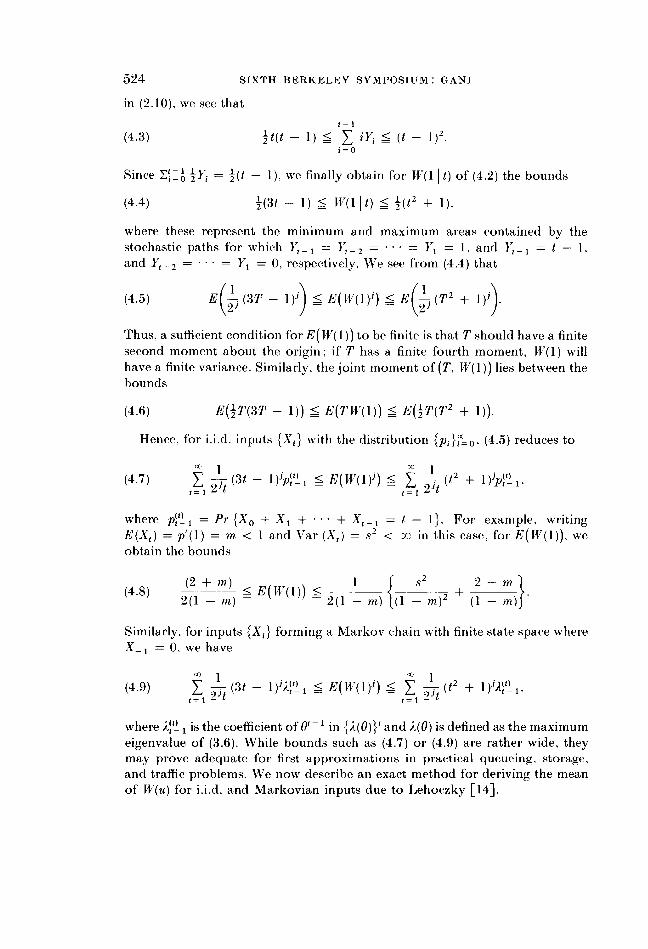
the joint moments of (T, W(1)), since, in summing the second set of inequalities


in (2.10), we see thatt- 1

(4.3) 2tt1) _ i i _ (t _1)2.i=o

Since Ei- = -(t- 1). we finally obtain for W(1 I t) of (4.2) the bounds

(4.4) -(3t - l) _ W(1 1t) < 1 (t2 + 1),

where these represent the minimum and maximum areas contained by thestochastic paths for which Y,-1 = Y2 = = Y1 = 1, and Y,,1= t- 1.and Y2= = Y1 = 0, respectively. We see from (4.4) that

(4.5) E 2J (3T- l)i) _ E(W(1)i) _ E2J (T2 + )J).

Thus, a sufficient condition for E(W(1)) to be finite is that T should have a finitesecond moment about the origin: if T has a finite fourth moment, W(1) willhave a finite variance. Similarly, the joint moment of (T, W(1)) lies between thebounds

(4.6) E('T(3T - 1)) . E(TW(1)) < E('T(T2 + 1)).

Hence, for i.i.d. inputs {Xi} with the distribution {pi}tt-o. (4.5) reduces to

(4.7) E 2' (3t - 1)jp,') 1 _ E(W(1)i) . (t2 + 1)jp4,.

where p,1i = Pr {X0 + X, + * + X, = t - 1}. For example. writingE(X,) = p'(l) = m < 1 and Var (X,) = s2 < cc in this case, for E(W(1)), weobtain the bounds

(2 ± rn) 1 $ 2 2-m(4.8) 2

<m-E( W( 1))-<

l { +2- }(.) 2(1 - m) -(() 2(1 - m) }(i M)2 (1 M)

Similarly, for inputs {Xi} forming a Markov chain with finite state space whereX_ 1 = 0, we have

10 1 "C 1(4.9) -J (3t - l)jA(,') 1 < E(W(1)i)-< J (t2 + 1j,)1

where i," 1 is the coefficient of Ot 1 in {2(O)}' and A(0) is defined as the maximumeigenvalue of (3.6). While bounds such as (4.7) or (4.9) are rather wide, theymay prove adequate for first approximations in practical queueing, storage,and traffic problems. We now describe an exact method for deriving the meanof W(u) for i.i.d. and Markovian inputs due to Lehoczky [14].


5. Exact results for the mean E(W (1))

Let us first consider the case of i.i.d. inputs {Xi}:. we follow Lehoczky's tech-nique [14] of conditioning the process on the input XO = i during the initialtime interval (0. 1), and so write the expectation of the path integral 11'(1) as

(5.1) E(W(1)) = 1 + Pi - + E(W(i))}.i=o 2

Now, from (1.4),

(5.2) E(W(i)) = Et {Wk + (i - k)Tk}) = iE(W(1)) + 'i(i - 1)E(T).

Hence substituting this in (5.1), we finally obtain

(5.3) E(W(1)) = 1 + m + E ipiE(W(1)) + , 4i(i - 1)piE(T).i=o o

or

(5.4) E(W(1)) = 1 + ! ( 21-rn 2(1-rn)2'

where E(X,) = m < 1, Var (X,) = s2 and E(T) = 1/(1 - m) as in Section 4.Thus for W(u), we find the expectation

(5.5) E(W(u)) = uE(W(1)) + u(u - 1)E(T) = u + }

The technique may be applied equally well to Markovian inputs {Xi} withfinite or denumerable state space. Assume as usual that the input X_ in thetime interval (- 1, 0) is zero, and for convenience allow the number of states inthe chain to be denumerably infinite. Then, once again conditioning on theinput XO = i during the interval (0. 1), we obtain

(5.6) E(W0(1)) = 1 + E poif{i + E(Wi(i))} = 1 + m + , poiE(Wi(i))i=o i=o

where mo = l'S. 0 ipoi < 1, and the subscripts in WO(1) and Wi(i) indicate thatthe inputs prior to the start of the two processes are 0 and i, respectively. Nowfor any prior input j, considering the first descent to state i - 1 of a processstarting from state i, we obtain

(5.7) E(^J(i)) = E(WV(1)) + (i - 1)E(Tj) + E(Wo(i - 1))= E(1V(1)) + (i - l)E(Tj) + (i - 1)E(Wo(I))

2(i - 1)(i - 2)E(T),

where Tj now denotes the time to first emptiness starting from state 1 withprior inputj, and we decompose WO(i - 1) according to (1.4).


Thus, we may rewrite (5.6) as

(5.8) E(Wo(1))

= 1 + Ymo+ pPoi{E(Wi(l)) + (i - 1)E(Wo(l))i=O

+ (i - l)E(Tj) + j(i- 1)(i - 2)E(T)}

= 1 + 2mO + (MO- 1)E(WO (1)) + E(T) Z 2(i - 1) (i - 2)poii-o

+ Z poiE(Wi(1)) + E (i 1)poiE(Ti).i=0 i=o

More generally, for Wk(1) starting from state 1 with prior input k and usingprecisely the same arguments, we have that

(5.9) E(Wk(I)) = 1 + 2mk + (mk - 1)E(WO(1)) + E(T) Z 2(i - 1)(i - 2)Pkii=0

+ Z PkiE(Wi(I)) + Y (i - 1)pkiE(Ti'),i=o i=0

where ik = ELT= 0 iPki < 1. Thus, expressing these results in matrix form, weobtain

(5.10) E(W(1)) = 1 + 'm + (m - 1)E(Wo(I)) + pE(W(1)) + R,

where W(1), 1, and m are column vectors with kth elements Wk(l), 1, and Mik,respectively, and R is the column vector with kth elements

OD 00~~~~~~~~~O

(5.11) E(T) Z 2(i - 1)(i - 2)Pki + Z (i - 1)PkiE(Ti).i=0 i=o

Note that E(T) and E(Ti') can be found from the p.g.f. g(6; 1, 0) and g(6; 1, i)of Section 3, so that R is assumed to be known.

If the Markov chain considered is stationary, E(WO(1)) = E(W(1)) can beobtained without difficulty. Rewriting (5.10) as

(5.12) {I - p}E(W(1)) = 1 + 'm + (m - 1)E(Wo(I)) + R

and premultiplying by the row vector n' of stationary probabilities {7rk}, weobtain

(5.13) n'{1 + 4m} + nc'(m- 1)E(WO(I)) + n'R = 0.

Hence, 00 0

1 + I1rimi +(5.14) E(WO(1)) i=0 i=0

1 - Irimii=0


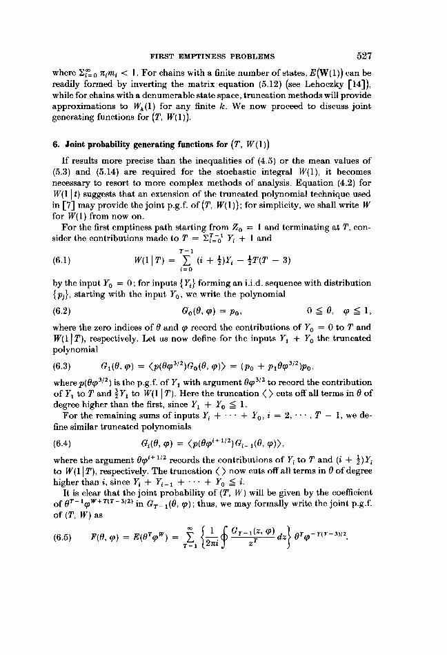
where E, 0 nimi < 1. For chains with a finite number of states, E(W(1)) can bereadily formed by inverting the matrix equation (5.12) (see Lehoczky [14]),while for chains with a denumerable state space, truncation methods will provideapproximations to Wk(l) for any finite k. We now proceed to discuss jointgenerating functions for (T, W(1)).

6. Joint probability generating functions for (T, W(1))

If results more precise than the inequalities of (4.5) or the mean values of(5.3) and (5.14) are required for the stochastic integral W(1), it becomesnecessary to resort to more complex methods of analysis. Equation (4.2) forW(1 It) suggests that an extension of the truncated polynomial technique usedin [7] may provide the joint p.g.f. of (T, W(1)); for simplicity, we shall write Wfor W(1) from now on.For the first emptiness path starting from ZO = 1 and terminating at T, con-

sider the contributions made to T = ET-7 Yi + 1 andT-1

(6.1) WQ 1 T) =E(i + ')Yi - T(T -3)i=o

by the input YO = 0; for inputs {Yi} forming an i.i.d. sequence with distribution{pj}, starting with the input YO, we write the polynomial

(6.2) G0(0 (P) = Po, 0 _ 0, U < 1,

where the zero indices of 0 and qp record the contributions of YO = 0 to T andW(1 | T), respectively. Let us now define for the inputs Y1 + YO the truncatedpolynomial

(6.3) G1(0, p) = (p0p93/2)G0(0, A')> = (Po + P10(P312)Po,where p(0gp312) is the p.g.f. of Y1 with argument 0'3/2 to record the contributionof Y1 to T and 3 Y1 to W(1 | T). Here the truncation < > cuts off all terms in 0 ofdegree higher than the first, since Y1 + YO _ 1.For the remaining sums of inputs Yi + * + YO, i = 2, , T - 1, we de-

fine similar truncated polynomials

(6.4) Go(0p ) = <P(OqPi+112)G 1(0, q,)>

where the argument 0(p'1/2 records the contributions of Yi to T and (i + 2)Yito W( 1| T), respectively. The truncation < > now cuts off all terms in 0 of degreehigher than i, since Yi + Yi- 1 + * * * + Yo _ i.

It is clear that the joint probability of (T, W) will be given by the coefficientof OT-1W+T(T-3/2) in GT-1(0 p); thus, we may formally write the joint p.g.f.of (T, W) as

(6.5) F(O, () = E(OT ) = E j G T dz} P T


where i = 1 and z is now a complex variable. Note that the integral mustbe taken on a suitable contour around the origin, and that (-T(T-3)/2 providesthe appropriate correction to the contributions of the {Y,} to W(1 | T).When the inputs {Yi} form a Markov chain with transition matrix {pij},

assumed to be infinite, we may write for the input YO the vector

P00

(6.6) Go( (p) = [Pio1 O 0, ( ,

where the zero indices of 0 and (p record the contributions of YO = 0 to T andW(1 | T), respectively. We now define for the sums of inputs Yi + + YO theith vector of truncated polynomials

POO P010(PiL+ 1/2 P02((Pi + 1/2)2 ...

(6.7) G1(O, 9) =< P10 P1 i+ 1/2 Al2(A0i+ 1/2)2 ... Gi- 1(0, (p)>.

where for i = 1,*, T - 2, the argument 09i+ 1/2 records the contributions ofYi to T and (i + 1)Yi to W(1 IT), respectively. The truncation <> cuts off allterms in 0 of degree higher than i, since Yi + Yi- 1 + Y+.o i; it followsin practice that one can neglect all elements of the matrix {Pkj(0i + 1/2 j} beyondthose of the (i + 1)th column and (i + 2)th row. Starting with GO(0. (P), thismeans we need only consider its first two elements [P].

Finally, since we assume once again that the input prior to the start of theprocess is X_ 1 = YT = 0, the truncated polynomial

(6.8) GTl- 1 (0 (P ) = <[Poo,polOpT-1,1*.. ,POT(-91( ]GT-1/2 )2T-(O]G ,(9)>will provide in the coefficient of OT- 19W+T(T-3)/2 the joint probability of(T, W). Hence, as before, we may formally write the joint p.g.f. of (T, W) as

(6.9) F(O, 9) = E(OT9W) = E T- 1( (P)dz9OT)-T(T-3)/2T=1 (22t J ZT z.09TT3/where z is a complex variable and the integral is taken on a suitable contour

around the origin. For a finite (r + 1) x (r + 1 ) matrix {pij}i j=o and a finitestate space, the same methods apply with appropriate modifications fromG, 1 (0, () onwards, due to the finiteness of the transition probability matrix.As simple illustrations of these techniques, we consider the following two

random walks.EXAMPLE 6.1. Let the {Xi} be i.i.d. with p(O) = pO + q, forO < p < 1 and

p + q = 1. In this case W = 2(3T - 1) and the joint p.g.f. of(T, W) is


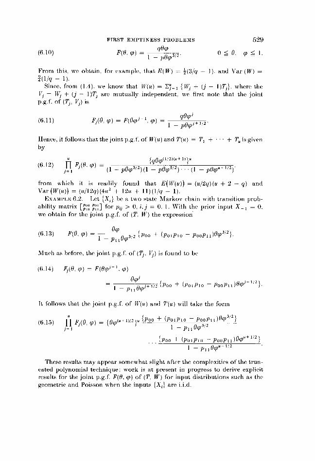
(6.10) F(0, ) = p 0 0, .< 1.

From this, we obtain. for example, that E(RW) = (3/q - 1), and Var (W) =49(l/q- 1).

Since, from (1.4), we know that W(u) = Y"=> {Wj + (j - 1)Tj}, where theVj = Wj +±(j-)Tj are mutually independent. we first note that the jointp.g.f. of (Tj, Vj) is

(6.11) Fj(0, () = F(0i',, p) = -0_po9p+1/2'Hence, it follows that the joint p.g.f. of IW(u) and T(u) = T1 + * + T. is givenby

(6.12) 11 Fj(O. 9) = (1 - pO312) {q09l_ +1)}..U+1/2

from which it is readily found that E(W(u)) = (u/2q)(u + 2 -q) andVar (W(u)) = (u/12q)(4u2 + 12u + 11)(1/q - 1).EXAMPLE 6.2. Let {Xi} be a two state Markov chain with transition prob-

ability matrix [~Po Pot] for pij > 0, i,j 0, 1. With the prior input X1 = 0.we obtain for the joint p.g.f. of (T. W) the expression

(6.13) F(O. )( 1 -P03 2 {poo + (PoiPio - PooPll)09312}.

Much as before, the joint p.g.f. of (Tj. Vj) is found to be

(6.14) Fj(O, () = F(091-'. ()

l_ 09J±1/2 {Poo + (PolPio -poop, )0pi+ 12}

It follows that the joint p.g.f. of W(u) and T(u) will take the form

(61U

E(,)-{0(+)2}u {poo ± (PoiPio - PooPii)O93112}6.1) fl, Fj ( 0, (p) = { 0?o( +3/2u{~(olplOPoPl1)0 /

J= 1 1 - pilo931{poo + (PoiPio -POooP11)O0u+112}

1 - P110l +/2

These results may appear somewhat slight after the complexities of the trun-cated polynomial technique; work is at present in progress to derive explicitresults for the joint p.g.f. F(0, 9o) of (T, J') for input distributions such as thegeometric and Poisson when the inputs {Xi} are i.i.d.


7. Random walks imbedded in birth and death processes and an asymptotic result

Joint distribution problems for the analogous time to first emptiness T'(u)and stochastic path integral W'(u) have been investigated for birth and deathprocesses in continuous time by Gani and McNeil [10]. For these, the doubleLaplace transform of T'(u), W'(u) when the birth and death parameters are,respectively, A and Au, has been shown to be

(7.1) u(o, p) = E(exp {-ciT'(u) - flW'(u)})()2 Ju+2(2(f)L)-1)I ' Re c, p _ 0,

where v = (a + A + p)f31. From (7.1), it is possible to find the expectation ofW'(u), as well as the regression of W'(u) on T'(u).A similar approach is applicable to the discrete time random walk imbedded

in a birth and death process. This is the random walk starting from ZO = u withi.i.d. inputs {X,},' 1 of size + 1 arriving at times t - 0, such that its state attimes t = 1, 2, T(u) is

(7.2) Zt = (Zt-l + Xt),with ZT(U) = 0 for the first time. The probabilities that X, = + 1 and -1 are,respectively, p = A/(2 + i) and q = p/(2 + p). If Fu(6, A) = E(6T(u)qW(u)) isthe joint p.g.f. of (T(u), W(u)), it is readily seen for u > 1, considering the inputX, = +1 during (0,1), that

(7.3) Fu(0, 9() = 0(pu{pFu+i(0, 9) + qPu (0, A))},

where FO0(, ) is put equal to 1 for convenience.We can solve these difference equations by setting

(7-4) F (6,(0 = (06, (P), u =1, 2,

whence

(7.5) u(6, (p) 1-=p'= (112 (qp) 11209u

VPJ 1 _(qp)1/20"(pu p 4 (0 (p)

The function cu(6, 9p) may be identified as the ratio of two Bessel functions ofinteger order, of the first kind, so that

(7.6) X(, (p) - ( J)J1(2u(qp) 120u)

FIRST EMPTINESS PROBLE'MS 531

Hence,

Un u/2 u=J)nk(2k(qp) 110(p)(7.7) F.(O, = 1u j(()U2 1 4,_(21(qp) 1120(pk)j=11~

a rather complicated explicit expression, somewhat reminiscent of (7.1).The analogy between this random walk and the continuous time birth and

death process suggests that the asymptotic normality proved for (T'(u), W'(u))in [10] will extend not only to the imbedded random walk, but also to thegeneral random walk (1.1) with regular unit output previously considered. Infact, this is the case, as is proved in detail in a recent note by Gani and Lehoczky[9]. Briefly, one begins by showing that for i.i.d. inputs contributing to thestochastic integral

(7.8) W(u)= WV+ (j-l )Tj.j= 1

the normalized sum u - 3/2 E'= IWj tends to zero almost surely. It is then provedthat, as u - o, the normalized random variables

{ W(u)-u(u- 1)} {T(U) - u}

where pu = E(Tj) and U2 = Var (j), are jointly normally distributed with cor-relation coefficient p = 3/2. For large u, this means the asymptotic regressionof W(u) on T(u) will be known. I would conjecture that it might be possible toobtain sharper asymptotic results for the stochastic integral W(u).No account of the wide field I have tried to cover could hope to be entirely

complete; despite its condensed form, I hope this brief sketch of unansweredproblems in the area may encourage applied probabilists to work on them andfind their solutions.

REFERENCES

[1] M. X. ALM KHAN and J. GANI, "Infinite dams with inputs forming a Markov chain." J. Appl.Prob., Vol. 5 (1968), Pp. 72-84.

[2] M. S. BARTLETT. "Equations for stochastic path integrals." Proc. Cambridge Philos. Soc.,Vol. 57 (1961), pp. 568-573.

[3] P. J. BROCKWELL and J. GANI.-"A population process with Markovian progenies." J. Math.Anal. Appl., Vol. 32 (1970). pp. 264-273.

[4] K. L. CHUNG, Markov Chains with Stationary Transition Probabilities, New York. Springer-Verlag, 1967.

[5] D. J. DALEY, "The total waiting time in a busy period of a stable single-server queue, I,'J. Appl. Prob., Vol. 6 (1969), pp. 550-564.

[6] D. J. DALEY and 1). R. JACOBS, "The total waiting time in a busy period of a stable single-server queue, 11," J. Appl. Prob., Vol. 6 (1969), pp. 565-;572.

[7] J. GANI, "Elementary methods for an occupancy problem of storage," Math. Ann., Vol. 136

(1958), pp. 454-465.


[8] 'A note on the first emptiness of (lams with Markovian inputs," J. Math. Anal.Appl.. Vol. 26 (1969). pp. 270-274.

[9] J. CANM and J. P. LEHOCZKY, 'An asymptotic result in traffie theory.'' Department ofStatistics Technical Report No. 23. Stanford University. 1970; J. Appl. Prob.. Vol. 8 (1971).pp. 815-820.

[10] J. CANi and D. R. MICNEIL. Applications of eertain birth-death and diffusion processes intraffic flow.'- D)epartment of Statistics Technical Report No. 17. Stanford University.1969: Adv. Appl. Prob., Vol. 3 (1971). pp. 339-352.

[11] 1. J. GOODn "The number of individuals in a cascade process," Proc. Cambridge Philos. Soc..Vol. 45 (1949). pp. 360-363.

[12] T. E. HARRIS, The Theory of Branching Processes, Berlin. Springer-Verlag, 1963.[13] D. G. KENDALL. "Some problems in the theory of (lams." J. Roy. Statist. Soc. Ser. B.

Vol. 19 (1957). pp. 207-212.[14] J. P. LEHOCZKY. "A note on the first emptiness time of an infinite reservoir with inputs

forming a Markov chain." J. Appl. Prob., Vol. 8 (1971). pp. 276-284.[15] E. H. I.OYD. "The epo('hs of emptiness of a semi-infinite discrete reservoir.' J. Roy. Statist.

Soc. Ser. B. Vol. 25 (1963). pp. 131-136.[16] "A probability theory of reservoirs with serially correlated inputs,' J. Hydrol..

Vol. 1 (1963). pp. 99-128.[17] "Reservoirs with serially correlated inflows." Technometrics. Vol. 5 (1963). pp.

85-93.[18] "Stochastic reservoir theory." Adcances in Hydroscience. Vol. 4. New York. Academic

Press. 1967.[19] E. H. LLOYD and S. ODOOM. "A note on the equilibrium distribution of' levels in a semi-

infinite reservoir subject to Markovian inputs and unit withdrawals." J. Appl. Prob.. Vol. 2(1965). pp. 215-222.

[20] 1). R. MCNEIL, "Integral functionals of birth and death processes and related limiting distri-butions." Ann. Math. Statist., Vol. 41 (1970). pp. 480-485.

[21] J. L. MOTT. "The distribution of the time to emptiness of a discrete dam under steady demand,"J. Roy. Statist. Soc. Ser. B. Vol. 25 (1963). pp. 137-139.

[22] P. S. PTaRI. "On the homogeneous birth-and-death process and its integral." Biomletrika.Iol. 53 (1966). pp. 61-71.

[23] "Some further results on the birth-and-death process and its integral," Proc. Cam-bridge Philos. Soc.. Vol. 64 (1968). pp. 141-154.

[24] I,. T'AKACS. "Investigation of waiting time problems by reduction to Markov processes,"Acta. Math. Acad. Sci. Hungar.. Vol. 6 (1955), pp 101-129.

[25] 1). VERE-JONES. "Ergodic properties of non-negative matrices. 1V" Pacific J. Math.. Vol. 22(1967). pp. 361-386.

[26] "Ergodic properties of non-negative matrices. 11." Pacific J. Math., Vol. 26 (1968).pp. 601-620.

first emptiness in queueing, storage, and traffic

Documents