Firms and Collective Reputation: a Study of theVolkswagen Emissions Scandal*

Rudiger Bachmann Gabriel Ehrlich Ying Fan

University of Notre Dame University of Michigan University of Michigan

CEPR, CESifo, and ifo CEPR and NBER

Dimitrije Ruzic Benjamin Leard

INSEAD University of Tennessee

September 20, 2021

Abstract

This paper uses the 2015 Volkswagen (VW) emissions scandal as a natural experiment

to provide evidence that collective reputation externalities are economically significant.

Using a combination of difference-in-differences and demand estimation approaches,

we document a spillover effect from the scandal to the non-VW German auto manufac-

turers. The spillover amounts to an average drop of $2,057 in consumer valuations of

these manufacturers’ vehicles and to a 34.6% reduction in their annual sales. We sub-

stantiate our interpretation that the estimates reflect a reputation spillover using data

on internet search behavior and direct measures of consumer sentiment from Twitter.

JEL Codes: D12, L14, L62.

Keywords: automobiles, collective reputation, demand estimation, difference-in-

differences, Google trends, reputation externalities, Twitter sentiment, Volkswagen

emissions scandal.

*We would like to thank Networked Insights for providing data, as well as seminar and confer-ence participants for helpful discussions. All errors are our own. E-mail contact: rbachman@nd.edu,gehrlich@umich.edu, yingfan@umich.edu, dimitrije.ruzic@insead.edu, or bleard@utk.edu. This version ofthe paper supersedes its first version titled “Firms and Collective Reputation: the Volkswagen EmissionsScandal as a Case Study” and published as CEPR-DP 12504 and CESifo-WP 6805 in December 2017.

“Collective reputations play an important role in economics and the social sciences. Countries,

ethnic, racial or religious groups are known to be hard-working, honest, corrupt, hospitable or

belligerent. Some firms enjoy substantial rents from their reputations for producing

high-quality goods.”

— Jean Tirole, 1996

1 Introduction

Reputation plays an important role in mitigating problems that arise from incomplete

information. While firms have individual reputations, groups of firms may also share col-

lective reputations. These collective reputations can come about through formal associa-

tions such as franchises or through informal associations such as country-of-origin labels,

for instance French wine, Swiss watches, or German engineering. With collective reputa-

tions come externalities: the action of one franchised store may affect the reputation of the

whole chain; similarly, an industrial scandal implicating one firm might spill over to other

firms in the industry. While such relationships among firms are common and frequently

in the public eye, measuring the externalities arising from collective reputations remains

challenging. In this paper, we identify and quantify the economic significance of collective

reputation externalities. We do so in the context of a major industrial scandal in the United

States, the 2015 Volkswagen (VW) emissions scandal.

In addition to being widespread, collective reputations merit attention both because

economists have often theorized that they play an important role in how the economy

functions, and because they raise questions about market discipline for firm misbehavior.

First, as Tirole (1996) notes, “Collective reputations play an important role in economics

and the social sciences,” and there is a well-developed theoretical literature on the topic.1

Nonetheless, the literature that empirically documents collective reputations among firms

and measures the resulting externalities remains thin. Second, the externalities arising

from collective reputation imply that firms may not fully bear the costs or reap the benefits

of decisions that affect the collective reputation of their group. In that sense, there may be

a public goods problem in which firms underinvest in behaviors that build and sustain col-

lective reputations. Conversely, firms may be insufficiently averse to engaging in behaviors

that, if discovered, would cause harmful reputational spillovers. The collective reputa-

tion externalities we document in this paper thus provide a counterpoint to the common

argument that consumer responses to firm misbehavior effectively discipline firms.1In addition to Tirole (1996), see for example Levin (2009) and Neeman et al. (2019).

1

A challenge in identifying and measuring collective reputation spillovers is that prod-

ucts are potentially substitutes. Consider a stylized example of a market with three firms.

Two firms share a collective reputation (e.g., VW and BMW are associated with “German

Engineering”) while a third does not (e.g., Ford). Suppose a negative shock harms the

reputation of the first firm and that the shock spills over to harm the reputation of the

second firm as well (e.g., misbehavior at VW tarnishes the reputation of “German Engi-

neering” and hence BMW). At the same time, substitution away from the first firm may

drive demand toward the second firm (BMW) as well as the third firm (Ford). These sub-

stitution effects generate two challenges to measuring the reputation spillover correctly.

First, no firm in the market is completely “untreated” by the shock. Second, the observed

change in sales for the second firm (BMW) is the combination of two potential effects: the

reputational spillover effect of interest and the substitution effect.

We overcome these challenges by combining difference-in-differences and structural

estimation approaches and by providing direct evidence on the scandal’s reputational con-

sequences in the United States. First, we use a difference-in-differences approach to show

that the VW emissions scandal reduced the U.S. vehicle sales of the non-VW German auto

manufacturers—BMW, Mercedes-Benz, and Smart—relative to their non-German coun-

terparts.2 We consider this result to be initial evidence that there was a country-specific

spillover from the VW scandal to the other German auto manufacturers. Second, we esti-

mate a model of vehicle demand with flexible substitution patterns to quantify the spillover

and the substitution effects separately. Third, we provide supplementary evidence that this

spillover effect is reputational in nature.

To relate the two approaches, we provide a framework to conceptualize the difference

between the difference-in-differences estimates and the true spillover effect of an indus-

trial scandal. We clarify how the two are related and provide conditions on the patterns of

substitution under which difference-in-differences results constitute evidence for the exis-

tence of a spillover effect. In our setting, the estimated patterns of demand confirm the

validity of these conditions. In other settings, researchers may lack the rich data needed

to estimate flexible substitution patterns but have supplementary information about these

patterns. Our framework establishes how and when difference-in-differences estimates

can indicate the existence of a spillover effect in those settings.

We find an economically significant reputational spillover from the scandal,

amounting to an average drop of $2,057 in consumer valuations of the non-VW German

manufacturers’ vehicles and a 34.6% reduction in those manufacturers’ annual U.S. unit

sales. The scandal’s total effect is smaller than its spillover effect because the spillover and

2Opel, a German auto manufacturer formerly owned by General Motors, does not sell in the United States.

2

substitution effects move in opposite directions. While the reputational spillover harmed

the non-VW German auto manufacturers, substitution away from VW benefited them. We

estimate that substitution away from VW led to an 11.0% increase in the other German

auto manufacturers’ unit sales, implying that the scandal’s net total effect (a 23.5% reduc-

tion in sales) was smaller than the reputational spillover on its own.

The finding that the spillover effect coexists with a countervailing substitution effect

away from VW—and that, therefore, the spillover effect is larger in absolute value than

the scandal’s combined effects—is unlikely to be a coincidence. Firms that are associated

closely enough to have a collective reputation (so that the spillover effect exists) are also

likely to produce close substitutes (which determines the substitution effect). Our results

show the economic importance of these spillovers and indicate that the spillovers can be

systematically undermeasured when substitution patterns are not taken into account.

We supplement our estimates of the scandal’s effects with Twitter data to document

changes in sentiment showing harm to the non-VW German automakers’ collective rep-

utation. These directly-observable changes in sentiment support our argument that the

estimated German-specific spillover was a reputational spillover. Moreover, we show pat-

terns of internet search behavior that cast doubt on an alternative interpretation of the

spillover effect that works through information rather than reputation. Finally, we provide

evidence that consumers at the time would have had no technical or economic reason to

believe that the other German auto manufacturers were implicated in the scandal.

The sudden revelation and intense media prominence of the VW emissions scandal, one

of the largest industrial scandals in recent history, make it an attractive natural experiment

to study spillovers from collective reputation. On September 18, 2015, the U.S. Environ-

mental Protection Agency (EPA) served a Notice of Violation to the VW Group alleging

that approximately 500,000 VW and Audi diesel-engine vehicles sold between 2009 and

2015 in the United States contained a defeat device allowing these vehicles to appear to

comply with emissions regulations in the test box, while having higher on-road emissions.3

For the general public, the scandal was a clear surprise in September 2015, and it immedi-

ately generated extensive media coverage. Moreover, the scandal occurred in an important

industry in the United States, of which German vehicles constitute a large share.4

The automotive sector is well-suited for the study of spillovers from collective reputa-

tion because of the salience of automotive brands, the existence of well-developed tools

for studying vehicle demand, and the richness of available data. In addition to individual

3The Volkswagen Group consists of Volkswagen proper plus Audi and Porsche.4In 2014, German auto manufacturers accounted for 8.1 percent of all U.S. light vehicle sales, making

Germany the second-largest source for foreign-branded vehicles.

3

automotive makes being salient to consumers, the German auto manufacturers featured

the notion of “German engineering” prominently in their U.S. advertising, creating a nat-

ural reputational group. To capture consumer substitution patterns across vehicles—and

thereby separate substitution from spillovers—we leverage the tools that the industrial

organization literature has developed for estimating vehicle demand. Our estimation pro-

cedure uses detailed data not only on vehicle sales and characteristics, but also surveys

that describe consumers’ demographics and their second-choice vehicles.5

Our work incorporates reputational spillovers in a large literature on demand estima-

tion in the auto industry (e.g., Berry, Levinsohn and Pakes, 1995; Petrin, 2002; Berry,

Levinsohn and Pakes, 2004; Train and Winston, 2007; Li, 2019; Springel, 2020; Grieco,

Murry and Yurukoglu, 2021; Xing, Leard and Li, 2021). We use a similar combination of

automotive and survey data to estimate our model as Grieco, Murry and Yurukoglu (2021),

who study the evolution of market power in the U.S. auto industry. Our discrete-choice

model allows consumers to value certain vehicle characteristics—such as a VW nameplate,

a diesel engine, or a non-VW German origin—differently before and after the VW scan-

dal. The coefficients on the latter two characteristics allow the scandal to have potential

spillovers on vehicles with diesel engines and on the German reputational group.

We also contribute to the literature on reputation by studying collective reputation and

by quantifying the reputation spillovers on the economic outcomes of firms. The focus

on group reputation distinguishes our paper from the literature on individual and plat-

form reputations, including Cabral and Hortacsu (2010), Li (2010), Mayzlin, Dover and

Chevalier (2014), Nosko and Tadelis (2015), Fan, Ju and Xiao (2016), Luca (2016), and

Li, Tadelis and Zhou (2020).6 Our paper also relates to work studying the reputational

effects of industrial scandals, such as Jonsson, Greve and Fujiwara-Greve (2009) for the

Swedish finance industry, Freedman, Kearney and Lederman (2012) for the U.S. toy indus-

try, Barrage, Chyn and Hastings (2020) for the British Petroleum oil spill, and Bai, Gazze

and Wang (2021) for the Chinese dairy industry.

Additionally, there is a small but growing literature that studies the consequences of the

Volkswagen emissions scandal. Strittmatter and Lechner (2020), Che, Katayama and Lee

5Specifically, we combine product-level data from WardsAuto with household-level survey data from amajor market research company. The addition of household-level data—which includes information ondemographics, actual purchase decisions, and second-choice purchase intentions—aids our estimation ofsubstitution patterns by providing direct information about: (1) which types of households purchase whichtypes of vehicles, and (2) which pairs of vehicles are close substitutes for particular households.

6There is also a finance literature that studies how a variety of corporate events adversely affect firmvalues and interprets such effects as reputational losses; see, for example, Fiordelisi, Soana and Schwizer(2014) for a summary of this literature. We have conducted a similar analysis using stock prices in a previousversion of the paper (Bachmann, Ehrlich, Fan and Ruzic, 2019). The analysis shows that the VW emissionsscandal reduced the cumulative abnormal stock returns of the non-VW German auto manufacturers.

4

(2018), and Ater and Yoseph (2020) study the scandal’s effect on Volkswagen vehicles in

the used car market. Griffin and Lont (2018) and Barth, Eckert, Gatzert and Scholz (2019)

investigate the financial market effects for VW and other large automakers. Alexander and

Schwandt (2019) use the scandal as a natural experiment to study the health effects of

vehicle exhaust. Relatedly, Ale-Chilet, Chen, Li and Reynaert (2021) study the German

auto manufacturers’ choice of the emission control technology underlying the scandal.

The remainder of the paper is organized as follows: Section 2 provides a more detailed

explanation and timeline of the VW emissions scandal and describes the scandal’s effect

on VW. Section 3 provides difference-in-differences estimates that indicate the existence

of a German-specific spillover effect from the scandal. Section 4 presents a model of

vehicle demand and quantifies the spillover effect. Section 5 provides support for our

interpretation of the spillover effect as a reputational spillover, and discusses alternative

interpretations. A final Section 6 concludes.

2 The VW Emissions Scandal as a Natural Experiment

In this section, we describe the timeline of the VW emissions scandal in more detail

and argue that it provides a good setting to study the spillovers arising from collective

reputation. Using data from print publications, the stock market, and social media, we

show that the scandal was largely unanticipated. We then provide evidence substantiating

the claim that German auto manufacturers share a group identity.

2.1 Timeline of the Scandal

In May 2014, West Virginia University’s Center for Alternative Fuels Engines and Emis-

sions found discrepancies between high on-road emissions by VW diesel vehicles and ear-

lier test results. The EPA and the California Air Resources Board (CARB) permitted a

voluntary recall of VW diesel vehicles in December 2014. In May 2015, CARB conducted

new tests, and again the on-road emissions failed to match the test-box results for VW

diesel vehicles. In July 2015, the agencies informed VW about these tests and threatened

not to certify the 2016 diesel vehicles. On September 3, 2015, VW admitted to the EPA

and CARB that it had used a defeat device in its software, which regulated emissions and

produced fake test results in the test box (see Breitinger (2018) for a more complete time-

line). The scandal entered its public phase on September 18, 2015, when the EPA served

a Notice of Violation to the Volkswagen Group.

Volkswagen’s culpability quickly became a matter of public knowledge: on September

5

20, two days after the start of the scandal, Volkswagen admitted publicly to the deception

and issued an apology. VW Chief Executive Officer Martin Winterkorn resigned three days

later, on September 23. He was eventually charged with fraud in the United States in

May 2018. On September 28, German authorities opened a fraud investigation of the

former CEO, and in October they authorized a police raid on the VW headquarters. The

U.S. Congress called the VW U.S. CEO Michael Horn to testify on October 8, 2015, and he

formally resigned his post in early March 2016. In anticipation of the fines and settlements

associated with the scandal, VW set aside more than $18 billion in fiscal year 2015. The

scandal’s legal resolution in the United States began in April 2016. On July 26, 2016, VW

and a U.S. court agreed on a civil settlement totaling $15 billion.

Major news outlets across many countries covered the scandal and its aftermath. On

September 19, the morning after the scandal, the front page of the New York Times read:

“U.S. Orders Major VW Recall Over Emissions Test Trickery.” The Wall Street Journal used

a more accusatory tone: “Volkswagen Faked EPA Exhaust Test, U.S. Alleges.” Spiegel On-

line and Zeit Online, the online platforms of two major German newspapers, frequently

reported about the scandal, which also quickly spilled over into popular culture. For ex-

ample, on October 13, 2015, Paramount Pictures and Leonardo DiCaprio’s production

company announced that they had secured the rights to shoot a film about the scandal,

and on September 22, 2016, VW was awarded the satirical Ig Noble Prize in chemistry

(Improbable Research, 2016).

2.2 The Scandal Surprised the General Public

Monthly print media mentions of “Volkswagen” more than tripled in September 2015,

suggesting that the scandal came as a complete surprise to the general public. We quantify

the media prominence of the scandal using data from the Newsbank news aggregator on

print media mentions of “Volkswagen” in the United States. The database covers roughly

5,000 U.S. newspapers, newswires, journals, and magazines. Figure 1 shows that men-

tions of “Volkswagen” spiked from a pre-scandal monthly average of 1,500 to 5,500 in

September 2015. This sudden increase suggests that the scandal caught the media and

public by surprise.

Along with the adverse attention in the media, VW’s stock price declined precipitously

following the EPA’s announcement; the visually evident discontinuity on September 18 in

Figure 2 suggests that the scandal came as a surprise to market participants. Volkswagen’s

end-of-day stock price fell by 33 percent in the two trading days following the scandal.

The stock price subsequently recovered some of its losses over the rest of the year, but at

6

Figure 1: Monthly Print Media Mentions of “Volkswagen” in the United States

010

0020

0030

0040

0050

0060

00C

ount

Jan. 2011 Jan. 2012 Jan. 2013 Jan. 2014 Jan. 2015 Jan. 2016Month

Note: Dashed line shows the month of the Volkswagen emissions scandal, September 2015. Data comefrom the Newsbank news aggregator, which covers roughly 5,000 U.S. newspapers, newswires, journals, andmagazines. Time period covered is January 2011 to August 2016.

the end of August 2016 it remained 24 percent lower than its pre-scandal closing price.7

Furthermore, the tone of social media discussion regarding Volkswagen suddenly

shifted, with positive sentiment declining and negative sentiment spiking in the aftermath

of the scandal. We document this pattern with novel sentiment measures from Networked

Insights.8 We focus on sentiment data from Twitter, an online social media networking ser-

vice where roughly 300 million active monthly users share short messages. The sentiment

measures in our data set are calculated from a 10 percent random sample from Twitter.

Networked Insights categorizes tweets as displaying positive, neutral, or negative senti-

ment toward the mentioned company. Posts are excluded from the analysis if they are not

written in English or if the user accounts are associated with locations outside the United

States. Networked Insights also constructs brand identifiers. An identifier for Volkswagen,

for instance, is meant to collate mentions of “Volkswagen,” “VW,” “#Volkswagen,” and the

7To focus on the effects within the United States and to avoid currency effects from the euro-based VWlisting on the Frankfurt Stock Exchange, we use the price of the VW American Depository Receipt (ADR)traded on U.S. markets. ADRs are issued by a U.S. depository bank, entitle the owner to shares in aninternational security and are priced and pay dividends in U.S. dollars.

8Networked Insights is a data analytics company, founded in 2006, that provides a platform for real-timesemantic analyses of social media posts; its primary clients are consumer-facing companies that use theplatform to manage their brands.

7

Figure 2: End-of-Day Stock Price for Volkswagen Group

2030

4050

60St

ock

Pric

e, D

olla

rs

Jan. 2011 Jan. 2012 Jan. 2013 Jan. 2014 Jan. 2015 Jan. 2016Day

Note: Dashed line shows the date of the Volkswagen emissions scandal, dated September 18, 2015. End-of-day price shown for Volkswagen ADR listed on U.S. stock exchanges. Data come from the Bloombergdatabase. Time period covered is January 2011 to August 2016.

like. Given the size of the underlying data set, Networked Insights only retains the past

13 months of data. We requested the data in September 2016, so our time series begins

on August 10, 2015, a little over a month before the scandal became public. We first cre-

ate average daily sentiment shares (positive/negative/neutral) for August 2015 for each

vehicle make in our data to serve as a pre-scandal baseline. We then construct sentiment

shares in excess of this August baseline for each day.

Figure 3 displays these sentiment metrics for VW and the VW Group two weeks before

and after the scandal. Panel A shows a decrease in positive sentiment toward VW, from

an average of 3 percentage points higher than its August baseline in the two weeks prior

to the scandal to an average of 8 percentage points below in the two weeks following

the scandal. Panel B displays a sharp increase in negative sentiment toward VW: from an

average of 3 percentage points below to an average of 26 percentage points above.9 The

results for the entire Volkswagen group (which includes Audi and Porsche) are similar.

Together, these two panels suggest that Volkswagen’s reputation suffered in the aftermath

of the September 18 EPA announcement.

9The pre-scandal and post-scandal means are statistically different at the 1 percent significance level forboth positive and negative sentiment.

8

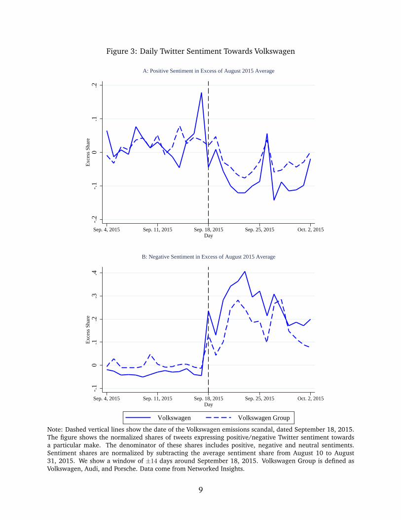
Figure 3: Daily Twitter Sentiment Towards Volkswagen

-.2

-.1

0.1

.2E

xces

s Sh

are

Sep. 4, 2015 Sep. 11, 2015 Sep. 18, 2015 Sep. 25, 2015 Oct. 2, 2015Day

A: Positive Sentiment in Excess of August 2015 Average

-.1

0.1

.2.3

.4E

xces

s Sh

are

Sep. 4, 2015 Sep. 11, 2015 Sep. 18, 2015 Sep. 25, 2015 Oct. 2, 2015Day

Volkswagen Volkswagen Group

B: Negative Sentiment in Excess of August 2015 Average

Note: Dashed vertical lines show the date of the Volkswagen emissions scandal, dated September 18, 2015.The figure shows the normalized shares of tweets expressing positive/negative Twitter sentiment towardsa particular make. The denominator of these shares includes positive, negative and neutral sentiments.Sentiment shares are normalized by subtracting the average sentiment share from August 10 to August31, 2015. We show a window of ±14 days around September 18, 2015. Volkswagen Group is defined asVolkswagen, Audi, and Porsche. Data come from Networked Insights.

9

2.3 “German Engineering” as a Group Identity

Having established that the VW scandal was a shock and that it affected VW’s reputa-

tion, we now provide evidence that there is a collective German reputation through which

the scandal may have had a spillover effect on the other German automakers.

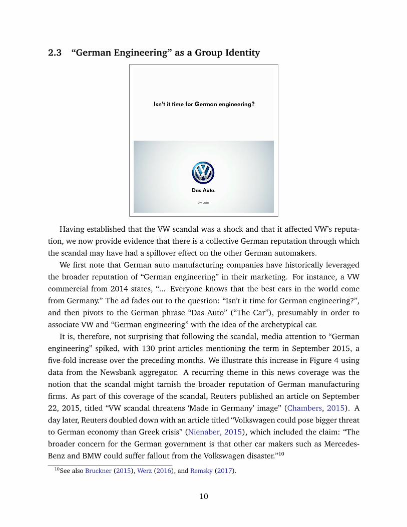
We first note that German auto manufacturing companies have historically leveraged

the broader reputation of “German engineering” in their marketing. For instance, a VW

commercial from 2014 states, “... Everyone knows that the best cars in the world come

from Germany.” The ad fades out to the question: “Isn’t it time for German engineering?”,

and then pivots to the German phrase “Das Auto” (“The Car”), presumably in order to

associate VW and “German engineering” with the idea of the archetypical car.

It is, therefore, not surprising that following the scandal, media attention to “German

engineering” spiked, with 130 print articles mentioning the term in September 2015, a

five-fold increase over the preceding months. We illustrate this increase in Figure 4 using

data from the Newsbank aggregator. A recurring theme in this news coverage was the

notion that the scandal might tarnish the broader reputation of German manufacturing

firms. As part of this coverage of the scandal, Reuters published an article on September

22, 2015, titled “VW scandal threatens ‘Made in Germany’ image” (Chambers, 2015). A

day later, Reuters doubled down with an article titled “Volkswagen could pose bigger threat

to German economy than Greek crisis” (Nienaber, 2015), which included the claim: “The

broader concern for the German government is that other car makers such as Mercedes-

Benz and BMW could suffer fallout from the Volkswagen disaster.”10

10See also Bruckner (2015), Werz (2016), and Remsky (2017).

10

Figure 4: Monthly Print Media Mentions of “German Engineering” in the United States

050

100

150

Cou

nt

Jan. 2011 Jan. 2012 Jan. 2013 Jan. 2014 Jan. 2015 Jan. 2016Month

Note: Dashed line shows the month of the Volkswagen emissions scandal, September 2015. Data comefrom the Newsbank news aggregator, which covers roughly 5,000 U.S. newspapers, newswires, journals, andmagazines. Time period covered is January 2011 to August 2016.

3 Difference-in-Differences Evidence on the Spillover Effect

In this section, we present difference-in-differences evidence that the VW emissions

scandal indeed had a spillover effect on the other German auto manufacturers (BMW,

Mercedes-Benz, and Smart). We show that the scandal substantially reduced the U.S. sales

growth of the other German automakers relative to their non-German counterparts. We

then interpret our difference-in-differences estimates through the lens of a general demand

system to clarify how they relate to spillovers.

3.1 Regression Results

To study the effects of the VW emissions scandal, we obtain data on U.S. light vehicle

sales from WardsAuto. WardsAuto receives sales data from all auto manufacturers in the

United States. It is thus in principle a complete count of light vehicle sales in the United

States.11 An individual observation in the data contains identifiers for the vehicle make

(e.g., Honda or Volkswagen), the vehicle model (e.g., Civic or Jetta), and the vehicle11The official U.S. vehicle sales statistics in national accounting data are based on the same data we use.

11

powertype (e.g., gas or diesel). The estimation uses data on 37 makes, listed in appendix

Table A.1, and 357 distinct models. The sample period is January 2010 to August 2016.

We identify six makes as of German origin: Audi, BMW, Mercedes-Benz, Porsche, Smart,

and Volkswagen.12

We use a difference-in-differences regression specification to show how the scandal af-

fected German auto manufacturers relative to the non-German auto manufacturers. We

begin the analysis by constructing a total sales measure for each make, so that an obser-

vation is a make-month (e.g., Honda in January 2016). Following a standard difference-

in-differences regression specification (e.g., Angrist and Krueger, 1999), we estimate the

following regression:

ykt = ηk + γt + ρTkt + εkt, (1)

where ykt = ln Saleskt − ln Saleskt−12 is the 12-month log sales growth rate of vehicle make

k at time t. ηk is a make-specific fixed effect, capturing potential make-level heterogeneity

in growth rates. γt is a fixed effect for each month in the sample, capturing potential

Figure 5: Differences in U.S. Light Vehicle Sales Growth

-.10

.1.2

.3Y

ear-

over

-Yea

r Log

Sal

es G

row

th

Jan. 2011 Jan. 2012 Jan. 2013 Jan. 2014 Jan. 2015 Jan. 2016Month

German excl. VW Group Non-German

Note: Dashed vertical line shows the month of the Volkswagen emissions scandal, September 2015. Datacome from WardsAuto. Volkswagen Group is defined as Volkswagen, Audi, and Porsche.

12Mini, the present-day incarnation of a line manufactured by the British Motor Corporation and its suc-cessors between 1959 and 2000, is currently owned by BMW. Given its historical association with Britain,we classify Mini as not of German origin. We consider alternative classifications in Appendix B.1 and showthat the results are not sensitive to this choice.

12

seasonality in vehicle sales and the potential impacts of time-varying fuel prices. Tkt is

an indicator taking value one for the German auto manufacturers during and after the

scandal month, and zero otherwise. The coefficient of interest, ρ, captures the scandal’s

differential impact on non-VW German auto manufacturers relative to non-German auto

manufacturers.

We exclude the Volkswagen Group from the sample to focus the analysis on the eco-

nomic consequences of reputation for German automakers not directly implicated by the

scandal. We weight this regression by the square root of sales volumes to dampen the

impact of highly volatile sales growth rates of small sales levels. Figure 5 shows that the

pre-scandal trends in sales growth for the non-VW German and non-German auto man-

ufacturers were comparable.13 Figure 5 also shows that the sales growth of the non-VW

German manufacturers turned negative following the scandal, offering a first indication

that there was an adverse spillover effect from the scandal.

The estimation results in Table 1 show that the scandal reduced the sales growth rates

of the non-VW German automakers by 9.2 percentage points relative to their non-German

counterparts (column 1). Given the scandal’s origins in the diesel market, a natural con-

cern is that this estimated effect could be driven by substitution away from diesel vehicles,

Table 1: Difference-in-Differences EstimatesGerman vs. Non-German Auto Manufacturers, Excl. VW Group

Dependent Variable 12-month Log Sales GrowthPower Type Baseline non-Diesel

(1) (2)

German × Post-Scandal -0.092∗∗∗ -0.084∗∗

(0.030) (0.033)

Time Fixed Effects Yes YesMake Fixed Effects Yes YesR2 0.303 0.300N 2150 2150

Note: Unit of observation is a make-month (e.g., the log growth of all BMW sales from January2014 to January 2015). Time period covered is January 2011 to August 2016. Standard errorsclustered at the make level in parentheses. VW Group (VW, Audi, and Porsche) excluded from allregressions. VW emissions scandal dated September 18, 2015. Sales are measured in units sold.All regressions are weighted by the square root of sales volumes. Data come from WardsAuto.*** p < 0.01, ** p < 0.05, * p < 0.1.

13Appendix B.2 adds some additional evidence for this assessment.

13

especially given that German and non-German auto manufacturers differ in their exposure

to the diesel market. Columns (2) assuages such concerns by repeating the difference-in-

differences regression for non-diesel vehicle sales only. We find that the scandal reduced

German automakers’ sales growth of non-diesel vehicles by 8.4 percentage points relative

to that of the non-German auto manufacturers. These results suggest that substitution

away from diesel cannot, on its own, explain the scandal’s relative effects on the other

German automakers: an additional channel must have been at play.14

3.2 Interpreting the Difference-in-Differences Estimate

In this section, we propose a framework to clarify how difference-in-differences (DID)

estimates such as those in the previous section relate to the true spillover effect of an

industrial scandal. Although the DID approach may misestimate the true spillover effect

because of substitution, we provide a condition under which the DID estimate indicates

that a spillover exists. We argue that this condition is likely to apply in many settings in

which researchers use scandals to study spillovers from collective reputations.

We consider a market with three groups of firms producing potentially substitutable

products: first, the “source” firm, which is directly implicated in scandalous behavior;

second, a group of “treated” firms, which are not directly implicated but which share

a collective reputation with the source firm; and third, a group of “comparison” firms,

which are not implicated in the scandal and do not share a collective reputation with the

source firm. Let θsource and θspillover denote, respectively, the deterioration of the source

and treated firms’ reputations following the scandal.

In what follows, we write demand for firm k’s products as qk(θsource, θspillover). Implicitly,

the demand function qk depends on each individual firm’s and its competitors’ product

prices and characteristics as well as consumer demographics and incomes. We suppress

this dependence in the notation in this section for expositional simplicity. We assume the

following properties of the demand function:

∂qk∂θsource

≥ 0 for all k ∈ treated, comparison (2a)

∂qk∂θspillover

≤ 0 for all k ∈ treated, ∂qk∂θspillover

≥ 0 for all k ∈ comparison. (2b)

These properties are implications of any demand model in which products are substitutes,

so that a firm’s demand increases in its own reputation and decreases in its competitors’

14In Appendix B.3 we show that the relative decline in the non-VW German automakers’ sales holds foralternative econometric specifications such as an unweighted regression or calculating sales growth ratesrelative to the average of sales in consecutive periods.

14

reputations. Examples of models with potentially substitutable products include discrete-

choice demand models such as McFadden (1974) and models of monopolistic competition

such as Dixit and Stiglitz (1977).

What the DID Estimate Captures

Let yk = f(qk) be a strictly monotonic transformation of qk used as the dependent

variable in a DID regression. We define the true spillover effect Ωspillover that we would like

to measure as:

Ωspillover , meank∈treated

[yk(θsource, θspillover)− yk(θsource, 0)].15 (3)

By contrast, the differences-in-differences estimator ΩDID compares the change in treatedfirms’ outcomes before and after the scandal to the change in the comparison firms’ out-comes. The empirical DID estimates include controls for time-varying factors other thanthe scandal. Therefore, in this stylized framework, we can define the DID estimate asshown in equation (4), which can be decomposed into the four terms in equation (5):

ΩDID , meank∈treated

[yk(θsource, θspill.)− yk(0, 0)]− meank∈comparison

[yk(θsource, θspill.)− yk(0, 0)] (4)

=

(meank∈treated

[yk(θsource, θspill.)− yk(θsource, 0)

]︸ ︷︷ ︸

spillover effect on treatment group , Ωspillover

+ meank∈treated

[yk(θsource, 0)− yk(0, 0)

]︸ ︷︷ ︸substitution effect on treatment group , Ω2

)(5)

−

(mean

k∈comparison

[yk(θsource, θspill.)− yk(θsource, 0)

]︸ ︷︷ ︸substitution effect on comparison group due to θspill. , Ω3

+ meank∈comparison

[yk(θsource, 0)− yk(0, 0)

]︸ ︷︷ ︸

substitution effect on comparison group , Ω4

).

The first term, Ωspillover, is the spillover effect of interest, while the second and fourth

terms, Ω2 and Ω4, arise as consumers substitute away from the source firm; by inequality

(2a), they are both positive. The third term, Ω3, captures how the comparison group’s

demand changes as a result of the spillover’s harm to the treatment firms’ reputations;

both Ωspillover and Ω3 would be zero in the absence of a spillover.

This decomposition illustrates three challenges to inferring Ωspillover from ΩDID. First,

the comparison group may be treated by the shock (i.e., Ω3,Ω4 6= 0), so ostensibly “un-

treated” firms may not be appropriate controls for the treatment group. Second, substitu-

tion away from the source firm toward the treatment group will bias ΩDID away from find-

ing a spillover effect (i.e., Ω2 ≥ 0 by inequality 2a). Third, following the shock to the source

15If the spillover were defined in the absence of the “source” shock, i.e., setting θsource = 0 in equation (3),all of the arguments in this section would still apply. We need only to replace yk(θsource, 0) by yk(0, θspillover)in equation (5) and swap the labels for the Ω terms in each row.

15

firm, even if there were no true spillover effect (θspillover = 0 and thus Ωspillover = Ω3 = 0),

ΩDID may still be non-zero because of differential substitution patterns across the treat-

ment and comparison groups.

Relationship between DID Estimates and Spillovers

Despite these challenges, we provide an intuitive condition under which the ΩDID es-

timator guarantees the existence of a spillover even if it does not provide a quantitatively

accurate estimate of the spillover.

Assumption 1 The shock to the source firm, θsource, induces a larger substitution effect to-ward the treatment group than toward the comparison group (i.e., Ω2 > Ω4).

Proposition 1 Under Assumption 1, if the DID estimate is negative (i.e., ΩDID < 0), then thespillover effect exists (i.e., θspillover > 0 and Ωspillover < 0).

Proof. Assumption 1 (i.e., Ω2 > Ω4) implies that if ΩDID(= Ωspillover + Ω2 − Ω3 − Ω4) < 0,

then Ωspillover − Ω3 < 0. Note that inequalities (2b) imply that sign(Ωspillover) 6= sign(Ω3).

Therefore Ωspillover < 0 (and Ω3 > 0). By (2b) we also have that θspillover < 0.

We believe that Assumption 1 is natural in settings with collective reputations, because

products close enough to share a collective reputation are likely to be closer substitutes

than products from other groups.16 Although the U.S. auto market features rich data and

well-developed tools to study demand, researchers attempting to estimate firm reputation

spillovers in other settings may be less fortunate. Proposition (1) shows that, in those

cases, difference-in-differences estimation can indicate the existence of a spillover effect

under an assumption about substitution patterns, especially when researchers have sup-

plementary knowledge regarding likely substitution patterns.

In the next section, we estimate a model of vehicle demand that allows for flexible

substitution patterns, and we use it to quantify the VW emissions scandal’s spillover effects

separately from its substitution effects. Those estimates confirm Assumption 1 in the con-

text of the VW emissions scandal, i.e., substitution away from VW Group sales following

the scandal was disproportionately toward the other German auto manufacturers. There-

fore, in line with our Proposition 1, we argue that our difference-in-differences estimates

indicate the existence of a spillover effect from the scandal.16Under a stronger set of conditions, we can also discuss the quantitative relationship between ΩDID and

the true spillover effect, Ωspillover. Equation (5) shows that if the comparison group were not affected bythe scandal (i.e., Ω3 = Ω4 = 0), then ΩDID = Ωspillover + Ω2, where Ω2 ≥ 0. By continuity, if the firmsin the comparison group are weak substitutes to the source and treatment firms (so that Ω3,Ω4 ≈ 0), thenthe DID estimate ΩDID will be a lower bound for the scandal’s spillover harm to the treatment group (i.e.,ΩDID > Ωspillover, noting that a negative value of Ωspillover represents harm).

16

4 Quantifying the Spillover Effect: Demand Estimation

and Decomposition

In this section, we estimate a model of vehicle demand that features flexible substi-

tution patterns as a means of disentangling the spillover and substitution effects of the

VW emissions scandal. We use this model to decompose the scandal’s impact on the U.S.

sales of the non-VW German automakers into three potential forces: a substitution effect,

a spillover effect, and a diesel effect. We allow for a diesel effect in the model because of

diesel technology’s role at the center of the scandal.

4.1 Demand Model

We assume that U.S. households’ vehicle demand is described by a discrete-choice

model. The indirect utility that household i derives from purchasing a vehicle of make-

model-power type j (hereafter, product j) in year t is given by:

uijt = xjtβi + ξjt + εijt, (6)

where the vector xjt includes the price of product j in year t, key observable attributes of

each product such as miles per gallon and vehicle weight, and fixed effects for country of

manufacturer and power type. Of particular importance for our purposes, xjt also contains

three dummy interaction terms, 1+(Scandal Makej × Post-Scandalt), 1+(Other Germanj ×Post-Scandalt) and 1+(Dieselj × Post-Scandalt). These interaction terms allow for potential

changes in consumer valuations of makes in the VW Group, for spillovers to other German

makes, and for potential changes in consumer valuations of diesel engines.17 The term

ξjt captures product characteristics that are not observable to the econometrician but are

known to households and auto manufacturers. Finally, εijt is an idiosyncratic taste shock.

We normalize the utility of household i’s outside option of not purchasing a vehicle during

year t to ui0t = εi0t.

To flexibly capture substitution patterns, we allow households to have heterogeneous

tastes with respect to product prices and characteristics. Specifically, we assume that the

coefficient vector βi can vary with household demographics di such as income and house-

hold size, so that βi = β + φdi.17The product-level dummy variables Scandal Makesj , Other Germanj , and Dieselj take the value 1 if,

respectively, product j belongs to the Volkswagen group, other German makes, or uses diesel fuel, and takethe value 0 otherwise. The time-varying dummy variable Post-Scandalt takes the value 1 if year t is after thescandal and 0 before the scandal.

17

We also allow households’ idiosyncratic tastes to be correlated across products. Specif-

ically, we assume that idiosyncratic tastes εijt follow a Generalized Extreme Value distri-

bution that allows for correlation in εijt for products of the same country origin.18 Let

λ ∈ [0, 1) be the within-country correlation parameter. A λ equal to zero represents the

case of no differential correlation. Positive estimates of λ would suggest that idiosyncratic

tastes are more closely correlated for products that share a common country origin.

To derive choice probabilities for households and market shares for products, we first

define the mean utility over all households that purchase product j in year t as:

δjt = xjtβ + ξjt. (7)

We denote by Jt the set of products available in year t, by Jgt the set of products with

country origin group g, and by (δt,xt) the collection of (δjt, xjt) for all j ∈ Jt. The prob-

ability that household i chooses product j of group g is Pr(uijt ≥ uij′t, ∀j′ ∈ Jt), which is

given by:

Prjt(δt,xt, di;φ, λ) =exp(δjt + xjtφdi)/(1− λ)

Iλigt[1 +∑

g′ I(1−λ)ig′t ]

, (8)

where Iigt =∑j′∈Jgt

exp(δj′t + xj′tφdi)/(1− λ).

Aggregating this choice probability using the distribution of demographics di across house-

holds, denoted by Gt(di), gives the market share of each product as follows:

sjt(δt,xt;φ, λ) =

∫Prjt(δt,xt, di;φ, λ)dGt(di). (9)

In Section 4.2, we describe how we map this model market share to the data as a means

of estimating the key model parameters. We also use this market share function for quan-

tifying the effects of the scandal in Section 4.3.

4.2 Data and Estimation

4.2.1 Combining Product and Household Data

To estimate our model of vehicle demand, we combine sales and characteristic data

at the product-year level from WardsAuto and survey data at the household level from a18In other words, εijt follows a nested Logit structure where a group (nest) consists of products with the

same country origin: Germany, Japan, Korea, United States, and All Other country origins. The outsideoption is its own group.

18

major market research company. As noted, a product in our analysis is a make-model-

power type combination (e.g., a Honda Civic with a gasoline engine). We define market

size by the number of households in the United States, and we use the all-items Consumer

Price Index for all urban consumers published by the Bureau of Labor Statistics to express

prices in constant 2015 dollars.

The WardsAuto data provide information on unit sales, prices (manufacturers’ sug-

gested retail prices), and key product attributes for all products between 2010 and 2016.

While the sales volume data is at the monthly frequency, the product characteristics data

(including prices) is at the annual frequency. Consequently, following much of the broader

literature on estimating vehicle demand, we estimate the model at the annual frequency.

Because the VW emissions scandal became public in September 2015, we define all years

prior to 2015 as the pre-scandal period and 2016 as the post-scandal period; we exclude

2015 from our estimation sample. Furthermore, the vehicle characteristics data are re-

ported at the product-trim level, while the sales volume data are at the product level. We

thus aggregate the characteristics data by taking the minimum across trims within each

product. As a robustness analysis, we also consider the median across trims. Appendix C.1

provides summary statistics of prices and product attributes.

Our household-level survey data provides information on households who have pur-

chased new vehicles. For each household in the dataset, we observe household demo-

graphics (i.e., household income, size, and the age of the respondent), the vehicle pur-

chased and other vehicles considered (e.g., vehicle “most seriously considered”). Consis-

tent with the WardsAuto data, we use the survey data for the years 2010 to 2016.

4.2.2 Estimation Procedure

We carry out the estimation in two steps, as in Goolsbee and Petrin (2004) and Train

and Winston (2007). In the first step, we leverage the household-level data and use maxi-

mum likelihood to estimate the parameters that capture heterogeneity in consumer tastes:

φ, which governs how consumer tastes vary with demographics, and λ, the within-country

correlation of idiosyncratic taste shocks. We also obtain the mean utility δjt for each prod-

uct. In the second step, we use an instrumental-variables approach to regress mean utility

δjt on product characteristics xjt to obtain an estimate of β, the parameters that capture

the mean tastes of consumers.

To conduct the first step, we leverage the fact that households in the surveys report

both the vehicle they purchased as well as the vehicle that the household “most seriously

considered” to construct the likelihood function with which we estimate parameters φ and

λ. We interpret those two survey responses as the household’s first- and second-most pre-

19

ferred product choices (see Berry, Levinsohn and Pakes (2004) for a similar interpretation

of similar survey data from General Motors).19 Let j1i and j2

i represent household i’s first

and second choices, respectively. The joint probability of household i choosing j1i as its

first choice and j2i as its second choice is the probability that j2

i is a better choice than any

j′ 6∈ j1i , j

2i , minus the probability that j2

i is a better choice than any j′ 6= j2i . In other

words, the probability is Pr(uij2i t ≥ uij′t for ∀j′ ∈ Jt\j1i ) − Pr(uij2i t ≥ uij′t for ∀j′ ∈ Jt),20

where the latter is given by equation (8) and the former can be analogously computed

from the choice set excluding j1i . With a slight abuse of notation, we rewrite the choice

probability in (8) as Prj(δt,xt, di;Jt;φ, λ) to make its dependence on the choice set Jtexplicit. Then the likelihood of observing household i’s first two choices as j1

i and j2i is the

following difference:

Prj2i (δt,xt, di;Jt\j1i ;φ, λ)− Prj2i (δt,xt, di;Jt;φ, λ). (10)

Instead of maximizing the likelihood over the entire parameter space of (φ, λ, δ) di-

rectly, we invert out the vector of mean utilities δ(φ, λ) and search over the parameter

space (φ, λ). Specifically, we invert out the vector of mean utilities δ by matching the ob-

served market shares in the data and the market shares predicted by the demand model

(i.e., equation 9), in the spirit of Berry (1994) and Berry, Levinsohn and Pakes (1995).21

Let δt(φ, λ) be the solution to sjt(δt,xt;φ, λ) = sjt for all j ∈ Jt, where the right-hand side

is the observed market share. Plugging δt(φ, λ) into (10) yields the likelihood function for

estimation:

L(φ, λ) =∑t

∑i∈It

log(Prj2i (δt(φ, λ),xt, di;Jt\j1

i ;φ, λ) (11)

− Prj2i (δt(φ, λ),xt, di;Jt;φ, λ)),

where It represents the households in a specific year’s survey. We randomly sample 10,000

households from each year of the survey to form the likelihood function (11). This step

also produces estimates of the mean utilities δjt.

To conduct the second step, we regress the estimated mean utility of each product δjt19The survey data provides information on the third and fourth choices as well. Due to a large number of

missing observations for these choices, we use only the first- and second-choice data.20This is because the probability of household i choosing j1i and j2i as its first and second choices is

Pr(uij1i t ≥ uij2i t ≥ uij′t,∀j′ ∈ Jt\j1i ). This probability is equivalent to Pr(uij1i t ≥ uij2i t and uij2i t ≥uij′t,∀j′ ∈ Jt\j1i ), which can be written as the difference between Pr(uij2i t ≥ uij′t,∀j′ ∈ Jt\j1i ) andPr(uij1i t < uij2i t and uij2i t ≥ uij′t,∀j

′ ∈ Jt\j1i ). Note that the second term equals Pr(uij2i t ≥ uij′t,∀j′ ∈ Jt).

21We compute the expectation in equation (9) by drawing a sample of household characteristics di fromthe Current Population Survey (CPS) using the household CPS weights.

20

on its price and characteristics using equation (7) and thereby estimate β, the parameters

capturing the average taste. Because product prices may be correlated with their unob-

servable demand shocks (i.e., the error term ξjt in equation 7), ordinary least squares

estimation could lead to biased estimates. Consequently, we use an instrumental-variables

approach. Specifically, we construct instrumental variables based on the characteristics

of close competing products (Gandhi and Houde, 2019). In the oligopolistic market for

automobiles, the price of product j depends not only on its own product characteristics,

but also on the attributes of the other products available in the market, especially close

substitutes as measured by the distance in attributes. The correlation between the char-

acteristics of other products and the potentially endogenous price makes those products’

characteristics relevant instruments. Under the timing assumption that automakers decide

the characteristics of their products before the realization of the demand shocks, the char-

acteristics of other products are uncorrelated with product j’s demand shock. Appendix

C.2 presents the first-stage regressions and details the instrumental variables we use.

4.2.3 Estimation Results

Table 2 reports the estimation results. The estimates show that consumer utility de-

creases with a vehicle’s price and increases with a vehicle’s size, its fuel efficiency, and its

horsepower relative to size. We also find that price sensitivity decreases both with house-

hold income and with household age. Larger and older households tend to prefer larger

vehicles. These estimates are robust to different ways of aggregating characteristics across

a product’s trims: for our baseline results in column (1) we use the minimum characteris-

tic, and in column (2) we use the median characteristic. The results are robust across the

two aggregation methods, so we focus on the baseline in what follows.

The estimated coefficient on VW Group × Post-Scandal is negative (–0.486), implying

that the scandal reduced consumer valuations of VW vehicles. This coefficient equates to

an average decline of $3,057 in consumer valuations of VW Group vehicles.22

The estimated coefficient for Other German × Post-Scandal is also negative (–0.327),

implying that the scandal reduced consumer valuations of the other German manufactur-

ers’ vehicles by an average of $2,057. This estimated change in valuations reflects the

scandal’s spillover effect on the other German automakers.

We find little change in consumers’ tastes for diesel vehicles following the VW scandal.

22We compute this decline in consumer valuations based on the change in consumer utility from purchasinga VW product post scandal and the average price coefficient. The former is the coefficient of VW Group ×Post-Scandal, i.e., −0.486; the latter is the price coefficient averaged across demographics, which is 1.590.Since our price variable is denominated in $10,000, the implied decline in consumer valuations of VWproducts is −0.486× $10, 000/1.590 = $3, 057.

21

Table 2: Demand Estimation Results—U.S. Light Vehicle Sales

Trim Aggregation:Min Median

(1) (2)

Price ($10,000) -2.439∗∗∗ -1.932∗∗∗

(0.104) (0.062)Price × Income ($1m) 3.807∗∗∗ 3.531∗∗∗

(0.060) (0.070)Price × Income2 -1.382∗∗∗ -1.729∗∗∗

(0.092) (0.141)Price × Age 1.096∗∗∗ 0.917∗∗∗

(0.017) (0.017)ln Weight 5.319∗∗∗ 4.721∗∗∗

(0.444) (0.312)ln Weight × 1(Household Size≥3) 0.176∗∗∗ 0.171∗∗∗

(0.010) (0.010)ln Weight × Income -2.055∗∗∗ -2.543∗∗∗

(0.143) (0.144)ln Weight × Income2 -1.451∗∗∗ -0.544∗∗∗

(0.199) (0.191)ln Weight × Age 1.317∗∗∗ 1.270∗∗∗

(0.030) (0.043)Horsepower/Weight (HP/1000lb) 0.035∗∗∗ 0.025∗∗∗

(0.006) (0.004)ln Miles-Per-Gallon 1.521∗∗∗ 1.610∗∗∗

(0.164) (0.165)VW Group × Post-Scandal -0.486∗∗∗ -0.391∗∗

(0.159) (0.159)Other German × Post-Scandal -0.327∗ -0.413∗∗

(0.175) (0.165)Diesel × Post-Scandal 0.071 0.145

(0.241) (0.239)Nest parameter 0.395∗∗∗ 0.396∗∗∗

(0.002) (0.002)

Country Fixed Effects yes yesPower-Type Fixed Effects yes yes

Note: Column (1) uses the minimum characteristic across trims as the product characteristic,and Column (2) uses the median. A product is defined as a make-model-power type (e.g., aHonda Civic with a gasoline engine). Time period covered is 2010 to 2016, with 2015 omittedas the scandal year. Country Fixed Effects comprises indicators for German, Japanese, Korean,U.S., and All Other country origins. *** p < 0.01, ** p < 0.05, * p < 0.1.

22

The estimated coefficients are small and statistically insignificant. The finding that the

scandal changed consumer valuations of German vehicles more noticeably than the con-

sumer valuation of diesel is consistent with our results in Table 1, where our difference-in-

differences estimates are quantitatively similar whether we consider all vehicles or focus

on non-diesel sales.

The estimated nest parameter λ is 0.395, indicating that, conditional on vehicle charac-

teristics, consumers viewed vehicles within the same country grouping as closer substitutes

than vehicles across country groupings. Overall, our estimated demand model implies that

the decline in consumer valuations of the VW Group led to a 12% increase in the non-VW

German auto manufacturers’ sales, while Japanese, Korean, U.S., and “Other National Ori-

gin” makes saw unit sales increase by only 0.6% to 0.7%. These results indicate that Ger-

man vehicles are closer substitutes than vehicles of other national origins, consistent with

Assumption 1 from Section 3.2, which we used to interpret the difference-in-differences

results as indicating the existence of a German-specific spillover from the scandal.

On the whole, the estimation results suggest three channels through which the VW

scandal affected the sales of the non-VW German auto manufacturers. First, we estimate a

significant decline in consumer valuations of VW vehicles. In a market where differentiated

vehicles are (imperfect) substitutes, this decline in valuations drove sales away from VW

toward vehicles produced by other manufacturers. Furthermore, this force drove sales

disproportionately toward the other German auto manufacturers, because their vehicles

are closer substitutes to VW than are non-German vehicles. We refer to this increase in

sales as the “substitution effect.” Second, consumer valuations of the other German auto

manufacturers also declined, reducing their sales. We refer to this decline in sales as the

“spillover effect.” Third, we allow but find little support for the idea that the scandal

changed consumers’ taste for diesel vehicles. In the next section, we quantify the scandal’s

overall effects on the non-VW German manufacturers’ vehicle sales and revenues, as well

as the relative contributions of each of these channels.

4.3 Quantifying the Effects

We now quantify how the scandal and its individual channels shifted vehicle demand

for the non-VW German auto manufacturers. To do so, we consider the U.S. light vehicle

market from 2014, the year prior to the scandal, and simulate how vehicle sales would

have changed had one or more of the scandal’s effects been present. We hold the set of

products and their characteristics—including prices—fixed in this exercise. Our exercise is

thus akin to asking how far the demand curve shifts in a simple supply-demand diagram;

it is distinct from asking how the scandal affected equilibrium outcomes. We focus on

23

this demand quantification as a transparent way to isolate the VW emissions scandal’s

individual channels. We show in the appendix that our decomposition is robust to an

alternative quantification of the scandal’s effects that considers equilibrium outcomes.

Table 3 summarizes the design of the three main simulations we use to quantify the

scandal’s effects. As the scandal took place in 2015, the 2014 data reflect none of those

effects. In Simulation 1, we turn on all three channels by setting all three post-scandal

interaction dummies to one and then recompute vehicle sales. Comparing the simulated

sales and revenues from Simulation 1 to those in the data gives us the overall effect of

the scandal. In Simulation 2, we turn on only two channels of the VW scandal: the diesel

channel and the spillover channel. Specifically, we set to one the post-scandal interaction

dummies for changes in the consumer valuations of the non-VW German auto manufac-

turers and for changes in the consumer valuation of diesel; we leave as zero the remaining

interaction dummy for the change in consumer valuations for VW Group vehicles after

the scandal. The difference between Simulations 1 and 2 is therefore only in whether

substitution away from the VW Group is present; comparing outcomes for these two sim-

ulations thus quantifies the substitution effect. Simulation 3 allows for only one channel:

the spillover driven by the estimated change in consumers’ tastes for the non-VW German

auto manufacturers. The comparison between Simulations 2 and 3 isolates the diesel ef-

fect that is present in Simulation 2 but not in Simulation 3. Finally, because Simulation 3

includes only the country-specific spillover channel, the difference between Simulation 3

and the (pre-scandal) data quantifies the spillover effect.

Table 3: Simulation Designs

Simluation 1 Simulation 2 Simulation 3 Data

Substitution Effect yes no no noDiesel Effect yes yes no noSpillover Effect yes yes yes no

Table 4 reports the overall effects of the scandal on non-VW German auto manufactur-

ers and a decomposition of the overall effects into the three channels. Together, the scan-

dal’s three channels reduce the sales of non-VW German auto manufacturers by 165,965

units worth $7.7 billion, roughly 23.5% of their 2014 sales. This decline is driven by the

spillover effect, which lowers sales for the non-VW German automakers by 244,607 ve-

hicles and reduces their revenues by $11.2 billion. This effect is partially offset by the

substitution effect, which increases sales for the non-VW German auto manufacturers by

24

Table 4: Scandal’s Impact on Other German Manufacturers

Comparison Vehicle Sales Revenue($ billion)

Overall Scandal Simulation 1 − Data –165,965 –7.74–23.50% –23.66%

Substitution Effect Simulation 1 − Simulation 2 77,342 3.4410.95% 10.52%

Diesel Effect Simulation 2 − Simulation 3 1,300 0.060.18% 0.17%

Spillover Effect Simulation 3 − Data –244,607 –11.24–34.63% –34.35%

Note: Simulation designs are defined in Table 3. Revenue effects are expressed in 2015 dollars.

77,342 units worth $3.4 billion as consumers switch away from Volkswagen. The changes

in unit sales and revenue ascribed to the changing consumer valuation for diesel are much

smaller than the substitution and spillover effects. Because the spillover and substitution

effects move in opposite directions, and the diesel effect is quantitatively negligible, the

scandal’s total net effect is substantially smaller than the spillover effect individually.

Our finding that the spillover effect is significant and larger than the overall effect of

the VW scandal is robust to alternative decompositions of the scandal’s impact on vehicle

demand. The three simulations we consider in this section are not the only way to isolate

the scandal’s effects. For instance, in Table 4, we quantify the spillover effect by comparing

Simulation 3 (where only the spillover channel is active) with the data (where no channel

is active). However, the comparison of any two simulations that differ only in whether the

spillover channel is active would be a valid quantification. In principle, the non-linearity

of the demand model means that the order in which each channel is turned on or off could

affect the decomposition results. We detail all possible simulations and comparisons in

Appendix C.3. The possible ranges for the individual effect sizes over all possible decom-

positions, including the baseline decomposition presented in Table 4, are quantitatively

narrow. Therefore, we conclude that the order in which consider the individual channels

is practically unimportant for isolating their effects.

Our findings are also robust to quantifying the scandal’s effect on the equilibrium

change in vehicle sales rather than focusing on the change in vehicle demand. To quantify

25

the change in vehicle demand in this section, we hold the product prices fixed at the level

we observe in the data. In Appendix C.4, we repeat all simulations allowing firms to ad-

just prices. Doing so requires additional assumptions about the supply side of the model.

Specifically, we model firms as setting prices in a Bertrand competition and back out the

(constant) marginal cost for each product based on the first-order conditions with respect

to prices. We then recompute the equilibrium prices while turning on some or all of the

scandal’s channels, using the backed-out marginal costs. In this alternative quantification,

the equilibrium change in vehicles sold comes both from a shift in the demand curve and

from a movement along the demand curve. By contrast, the quantification in this section

isolates the scandal’s channels by restricting attention to changes in consumer demand.

Nonetheless, we obtain quantitatively similar effects from the alternative exercise.

5 Interpretation of the Spillover Effect

In this section, we argue that the most plausible interpretation of the spillover effect

documented and quantified in the previous two sections is that it arises from a collective

reputation shared by all German automakers selling vehicles in the United States. As men-

tioned in Section 2, German auto manufacturers used the notion of “German engineering”

in their advertising, providing prima facie evidence that they share a collective reputation.

Here, we begin by presenting more direct evidence that the VW emissions scandal led to

a deterioration in public perceptions of the other German automakers sharing a collective

reputation. We then discuss an alternative information-based interpretation and argue

that it is less persuasive. Finally, we describe subsequent scandals involving the German

automakers that occurred after the end of our analysis period, and thus conclude that these

subsequent scandals cannot explain our documented spillover effect.

We use the Twitter sentiment data described in Section 2.2 to show that perceptions of

the non-VW German automakers suffered in the aftermath of the VW emissions scandal.

Specifically, we estimate the difference-in-differences specification in equation (1) with

Twitter sentiment data for the non-VW German automakers. The unit of observation is a

make-day.23 Column (1) of Table 5 shows a statistically significant decline of 3.5 percent-

age points in positive sentiment toward non-VW German auto manufacturers as a result

of the scandal (we discuss the results for negative Twitter sentiment in column (2) later

23The Networked Insights database does not include identifiers for some makes in the WardsAuto data.Table A.2 in Appendix A lists the makes with Twitter sentiment data. The estimation sample is a window of±14 days around the scandal eruption date of September 18, 2015, and the outcome variable is the share oftweets expressing positive/negative Twitter sentiment towards a particular make. The denominator of theseshares includes positive, negative and neutral sentiments.

26

Table 5: Difference-in-Differences Estimates—Twitter SentimentGerman vs. Non-German Auto Manufacturers, Excl. VW Group

Dependent Variable Positive Sentiment Negative Sentiment

(1) (2)

German × Post-Scandal -0.035 0.002(0.006) (0.006)

Time Fixed Effects Yes YesMake Fixed Effects Yes YesR2 0.348 0.268N 840 840

Note: Unit of observation is a make-day. Sentiment shares are normalized by subtracting theaverage sentiment share from August 10 to August 31, 2015. The denominator of these sharesincludes positive, negative and neutral sentiments. The estimation period comprises 14 daysbefore and after scandal date of September 18, 2015. Volkswagen Group is defined as Volkswa-gen, Audi, and Porsche. All regressions include make and time fixed effects, and are weightedby tweet volume. Data come from Networked Insights.

in this section). To put this number in perspective, the share of tweets expressing positive

sentiment toward those companies averaged 12.3 percent in August 2015. We consider

this deterioration in positive social-media sentiment towards the other German automak-

ers as suggesting that the sales spillover effect we document arose from a country-specific

collective reputation.

An alternative interpretation of the spillover effect to the non-VW German auto man-

ufacturers is that, following the scandal, consumers suspected these other German auto

manufacturers of having engaged in cheating behavior similar to VW’s. Such a suspicion

could have arisen from a shared German identity, in which case this alternative channel

is ultimately connected to group reputation. If, however, such a suspicion arose from

independent information available to consumers around the time of the scandal, this al-

ternative interpretation would indeed be distinct from our notion of collective reputation.

We present three arguments against this alternative interpretation. Our first argument

provides evidence suggesting that any such “shared suspicion” was not substantiated by

information available to consumers around the time of the VW scandal. Our second ar-

gument is that patterns of social media sentiment are indeed inconsistent with consumers

possessing information that implicated the other German auto manufacturers in malfea-

sance similar to VW’s. Our third argument goes further and presents online search patterns

suggesting that consumers did not possess such suspicions in the first place.

27

First, there was no concurrent notion of malfeasance by the non-VW German automak-

ers. The West Virginia University study that ultimately led to the discovery of the VW

scandal focused on three diesel vehicles: a VW Passat, a VW Jetta, and a BMW X5. The

VW vehicles failed the test, whereas the BMW vehicle passed. No Mercedes-Benz vehicles

were tested (see Thompson, Carder, Besch, Thiruvengadam and Kappanna, 2014). In ad-

dition, Mercedes-Benz and BMW had little technical reason to resort to cheating devices,

as their diesel vehicles tended to be larger than VW’s. As a result, they used exclusively

the Selective Catalytic Reduction (SCR) system as their NOx-control system, which adds

urea and water to the exhaust flows. This system is more effective and more reliable in

reducing NOx emissions but requires more space for the urea and water containers. VW,

with on average smaller vehicles in its fleet, developed a different system, a nitrogen oxide

trap, which the VW engineers could never get to operate with the same efficiency as SCR

systems.24 This difficulty was what led to VW’s deception in the first place: VW would

not have been able to comply with U.S. regulations without cheating (Zycher, 2017). Fi-

nally, media at the time wrote that non-VW German automakers were not implicated in

the scandal. On September 22, 2015, for instance, CNN wrote (Petroff, 2015): “But before

you start worrying about the complete collapse of the German auto industry, it’s worth

repeating that—at least for now—the scandal is limited to Volkswagen. Other German

automakers such as Daimler, which owns Mercedes-Benz, and BMW have said they’re not

affected.” Even in the fall of 2017, Zycher wrote (Zycher, 2017): “Note that VW is the

only manufacturer accused of explicitly installing such systems to defeat NOx emissions

control systems. [...] In short, it is perverse to fail to distinguish between the behavior of

VW and that of the rest of the industry.”

Second, Twitter sentiment toward the other German automakers displayed a very dif-

ferent pattern after the scandal than did Twitter sentiment toward VW. As mentioned

in Section 2.2, negative sentiment toward VW increased sharply following the scandal,

while positive sentiment declined moderately. This evidence suggests that suspicion of

malfeasance manifests mainly as an increase in negative sentiment towards the wrong-

doer. Therefore, if consumers indeed had information that other German automakers were

cheating too, we should expect a similar pattern for their social-media sentiment. How-

ever, as shown in column (2) of Table 5, we find no meaningful change in negative Twitter

sentiment following the scandal for the other German automakers. By contrast, positive

sentiment toward them declined, as shown in column (1). This decline in positive senti-

ment without a corresponding increase in negative sentiment suggests that perceptions of

24Of the three tested vehicles, only the VW Passat had a SCR system installed, but, according to Zycher(2017), the system was operating with reduced efficiency to not inconvenience the driver with too frequentrefills of the urea.

28

non-VW German automakers suffered after the scandal for reasons other than consumers

possessing information about malfeasance.

Third, although online searches for Volkswagen spiked following the scandal, con-

sumers showed no heightened inquisitiveness toward the other German auto manufac-

turers. Figure 6 contains four panels, each of which plots a time series of a single Google

search term (“Volkswagen”, “VW”, “BMW”, and “Mercedes”).25 Searches for “Volkswagen”

and “VW” in panels A and B increased dramatically in the aftermath of the scandal, with

respective z-scores of 22 and 15 in the week of September 18, the date of the EPA an-

nouncement. By contrast, searches for the two main non-VW German makes, “BMW” in

panel C and “Mercedes” in panel D, are indistinguishable from their regular fluctuations.

The Google search data implies that consumers did not become more inquisitive about the

other German auto manufacturers following the scandal. If consumers suspected those

automakers of cheating similar to VW’s, they did not display it in a similar accompanying

search for information.

Taken together, these three arguments suggest that the scandal’s effects on non-VW

German automakers were unlikely to be driven by information. Rather, the scandal must

have tarnished the reputations of the other German auto manufacturers through their

association with Volkswagen, consistent with the notion of a collective reputation.

We conclude this section with a brief discussion of some scandals involving the Ger-

man auto manufacturers, clarifying both that they are unrelated to the 2015 VW emissions

scandal and that they erupted well after the end of our study period. In the summer of

2017, it was suggested that Mercedes-Benz had also manipulated emissions (Zeit Online,

2017), although Mercedes-Benz never admitted to wrongdoing in the United States. Note

that these accusations arose almost two years after the VW scandal broke and one year

after the end of our study period. Later, in the spring of 2018, BMW had its own cheat-

ing device scandal, which led to raids of its corporate offices in Germany (Ewing, 2018).

However, as Ewing (2018) also reports, this affair was much smaller (11 thousand vehicles

affected versus 11 million in the VW scandal). More importantly, it had no U.S. impact as

none of the affected vehicles were in the United States.26

25The underlying data on Google trends is weekly, and it id by Google so that 100 corresponds to thelargest number of searches per week in the search period. For weekly data, Google trends only allows usersto download a few pre-defined search periods. We chose a five-year window from August 2011 to August2016. We normalize the series and express weekly values as z-scores, deviations from the mean that arescaled by the standard deviation. A z-score of 1 indicates a 1-standard-deviation increase over the mean.Both the means and the standard deviations are constructed using the period prior to September 2015.

26Like Mercedes-Benz, BMW never admitted to any wrongdoing. BMW executives blamed a simple mistakethat led them to install the wrong software for the implicated vehicles. The subsequent fines imposed byGerman authorities were $11.6 million, orders of magnitude smaller than the combined $25 billion of finesfor VW in the United States and Germany (see Dobush, 2018).

29

Figu

re6:

Goo

gle

Tren

dsof

Sear

ches

for

Ger

man

Aut

oM

anuf

actu

ring

Firm

s

-50510152025Z-Score

Jan.

201

2Ja

n. 2

013

Jan.

201

4Ja

n. 2

015

Jan.

201

6W

eek

A. V

olks

wag

en

-50510152025Z-Score

Jan.

201

2Ja

n. 2

013

Jan.

201

4Ja

n. 2

015

Jan.

201

6W

eek

B. V

W

-50510152025Z-Score

Jan.

201

2Ja

n. 2

013

Jan.

201

4Ja

n. 2

015

Jan.

201

6W

eek

C. B

MW

-50510152025Z-Score

Jan.

201

2Ja

n. 2

013

Jan.

201

4Ja

n. 2

015

Jan.

201

6W

eek

D. M

erce

des

Not

e:D

ashe

dlin

essh

owth

ew

eek

ofth

eVo

lksw

agen

emis

sion

ssc

anda

l,da

ted

Sept

embe

r18

,201

5.Th

eun

derl

ying

data

onG

oogl

etr

ends

isw

eekl

yan

dit

issc

aled

byG

oogl

eso

that

100

corr

espo

nds

toth

ela

rges

tnum

ber

ofse

arch

espe

rw

eek

inth

esa

mpl

epe

riod

(Aug

ust2

011

toA

ugus

t201

6).

We

cons

truc

tz-

scor

esas

the

devi

atio

nfr

omth

em

ean

ofth

ese

ries

,nor

mal

ized

byit

sst

anda

rdde

viat

ion.

The

z-sc

ores

onth

eve

rtic

alax

isar

eco

nstr

ucte

dus

ing

the

mea

nan

dst

anda

rdde

viat

ion

for

each

sear

chte

rmov

erth

epe

riod

prio

rto

Sept

embe

r20

15.

30

VW, BMW, and Mercedes-Benz also encountered unrelated legal trouble with the Euro-

pean competition authority (BBC, 2018). The case concerned the standardization of parts,

which is legal under European competition law for efficiency purposes, as long as the coor-

dinating parties seek permission from the competition authorities; they appear not to have

done so in this case. In addition, the case was technologically unrelated to the emissions

scandal because it concerned not defeat devices but standardization of parts.27 Notably,

“The Commission said it had no indications that the automakers coordinated with each

other on the use of illegal emissions-cheating ‘defeat devices”’ (BBC, 2018).

To sum up: at the time that the VW scandal broke, U.S. consumers had neither a tech-

nical nor an economic reason to believe that BMW and Mercedes-Benz were culpable of

malfeasance similar to VW’s. The documented Google search behavior and Twitter senti-

ment expression appear to be inconsistent with the notions that BMW and Mercedes-Benz

were implicated in the same way as VW, nor that U.S. consumers believed in collective

malfeasance. By contrast, the evidence is consistent with our interpretation of the spillover

effect as arising from collective reputation.

6 Conclusion

This paper documents that firms have economically important collective reputations in

the context of a key industry featuring national powerhouse companies. Using the 2015

VW emissions scandal as a natural experiment, we show that these collective reputations

can give rise to reputation spillovers with large economic consequences; in particular,

a scandal implicating one group member can have adverse impacts on the other group

members not implicated in the wrongdoing. We begin by using a difference-in-differences

approach to show that the scandal reduced sales at the other German auto manufacturers

relative to their non-German counterparts. The net total effect of the scandal is a com-

bination of two countervailing forces, the substitution effect and the spillover effect. We

estimate a model of vehicle demand to decompose the scandal’s effect into its individual

channels. Our results suggest that the scandal had an economically important country-

specific reputational spillover. We thus provide empirical support for the existence both

of collective reputation for firms and of group reputation externalities and quantify their

economic significance.

27The standardization of parts occurred in two areas: particle filters for gas engine vehicles and ureacontainers for diesel engine vehicles (which VW had only used in a few of its larger vehicles).

31

References

Ale-Chilet, Jorge, Cuicui Chen, Jing Li, and Mathias Reynaert (2021), “Colluding against

environmental regulation.” Working Paper 16038, Center for Economic Policy Research.

Alexander, Diane and Hannes Schwandt (2019), “The impact of car pollution on infant and

child health: Evidence from emissions cheating.” WP 2019-04, Federal Reserve Bank of

Chicago.

Angrist, Joshua and Alan Krueger (1999), “Empirical strategies in labor economics.” In

Handbook of Labor Economcis (Orley Ashenfelter and David Card, eds.), volume 3, chap-

ter 23, 1277–1366, Elsevier.

Ater, Itai and Nir Yoseph (2020), “The impact of environmental fraud on the used car

market: Evidence from dieselgate.” Working Paper 12899, Center for Economic Policy

Research.

Bachmann, Ruediger, Gabriel Ehrlich, Ying Fan, and Dimitrije Ruzic (2019), “Firms and

collective reputation: A study of the Volkswagen emissions scandal.” Working Paper

26117, National Bureau of Economic Research.

Bai, Jie, Ludovica Gazze, and Yukun Wang (2021), “Collective reputation in trade: Evi-

dence from the chinese dairy industry.” Review of Economics and Statistics, 1–45.

Barrage, Lint, Eric Chyn, and Justine Hastings (2020), “Advertising and environmental

stewardship: Evidence from the BP oil spill.” American Economic Journal: EconomicPolicy, 12, 33–61.

Barth, Florian, Christian Eckert, Nadine Gatzert, and Hendrik Scholz (2019), “Spillover

effects from the Volkswagen emissions scandal: An analysis of stock, corporate bond,

and credit default swap markets.” Working Paper, Friedrich-Alexander-Universitat (FAU)

Erlangen-Nurnberg.

BBC (2018), “BMW, Daimler and Volkswagen face EU diesel emissions probe.” BBC. https:

//www.bbc.com/news/business-45558588.

Berry, Steven (1994), “Estimating discrete-choice models of product differentiation.” RANDJournal of Economics, 25, 242–262.

Berry, Steven, James Levinsohn, and Ariel Pakes (1995), “Automobile prices in market

equilibrium.” Econometrica, 63, 841–890.

32

Berry, Steven, James Levinsohn, and Ariel Pakes (2004), “Differentiated products demand

systems from a combination of micro and macro data: The new car market.” Journal ofPolitical Economy, 112, 68–105.

Breitinger, Matthias (2018), “Der Abgasskandal.” Zeit Online. http://www.zeit.de/wirtsc

haft/diesel-skandal-volkswagen-abgase.

Bruckner, Johanna (2015), “Was die Skandale fur das deutsche Image bedeuten.”

Sueddeutsche.de. http://www.sueddeutsche.de/kultur/pegida-dfb-und-vw-was-die-ska

ndale-fuer-das-deutsche-image-bedeuten-1.2732828.

Cabral, Luıs and Ali Hortacsu (2010), “The dynamics of seller reputation: Evidence from

eBay.” Journal of Industrial Economics, 58, 54–78.

Chambers, Madeline (2015), “VW scandal threatens ‘Made in Germany’ im-

age.” Reuters. https://www.reuters.com/article/usa-volkswagen-germany-image-idUSL

5N11S38X20150922.

Che, Xiaogang, Hajime Katayama, and Peter Lee (2018), “Willingness to pay for brand

reputation: Lessons from the Volkswagen emissions scandal.” Working Paper, Durham

University.

Dixit, Avinash K. and Joseph E. Stiglitz (1977), “Monopolistic competition and optimum

product diversity.” American Economic Review, 67, 297–308.

Dobush, Grace (2018), “BMW will pay $11.6 million in dieselgate fines—a tiny penalty

compared to other emission scandals.” Fortune Magazine. http://fortune.com/2018/09/

03/bmw-dieselgate-fine/.

Ewing, Jack (2018), “BMW offices raided by authorities in emissions-cheating investiga-

tion.” The New York Times. https://www.nytimes.com/2018/03/20/business/energy-e

nvironment/bmw-diesel-emissions.html.

Fan, Ying, Jiandong Ju, and Mo Xiao (2016), “Reputation premium and reputation man-

agement: Evidence from the largest e-commerce platform in China.” International Jour-nal of Industrial Organization, 46, 63–76.

Fiordelisi, Franco, Maria-Gaia Soana, and Paola Schwizer (2014), “Reputational losses and

operational risk in banking.” European Journal of Finance, 20, 105–124.

33

Freedman, Seth, Melissa Kearney, and Mara Lederman (2012), “Product recalls, imperfect

information, and spillover effects: Lessons from the consumer response to the 2007 toy

recalls.” Review of Economics and Statistics, 94, 499–516.

Gandhi, Amit and Jean-Francois Houde (2019), “Measuring substitution patterns in dif-

ferentiated products industries.” Working Paper 26375, National Bureau of Economic

Research.

Goolsbee, Austan and Amil Petrin (2004), “The consumer gains from direct broadcast

satellites and the competition with cable tv.” Econometrica, 72, 351–381.

Grieco, Paul, Charles Murry, and Ali Yurukoglu (2021), “The evolution of market power in

the U.S. auto industry.” Working Paper, Pennsylvania State University.

Griffin, Paul and David Lont (2018), “Game changer? The impact of the VW emission-

cheating scandal on the interrelation between large automakers’ equity and credit mar-

kets.” Journal of Contemporary Accounting & Economics, 14, 179–196.

Improbable Research (2016). Improbable Research. http://www.improbable.com/ig/winn

ers/.

Jonsson, Stefan, Henrich Greve, and Takako Fujiwara-Greve (2009), “Undeserved loss:

The spread of legitimacy loss to innocent organizations in response to reported corporate

deviance.” Administrative Science Quarterly, 54, 195–228.

Levin, Jonathan (2009), “The dynamics of collective reputation.” The B.E. Journal of The-oretical Economics (Contributions), 9, Article 27.

Li, Jing (2019), “Compatibility and investment in the U.S. electric vehicle market.” Work-

ing Paper, MIT.

Li, Lingfang (2010), “Reputation, trust, and rebates: How online auction markets can

improve their feedback mechanisms.” Journal of Economics & Management Strategy, 19,

303–331.

Li, Lingfang, Steven Tadelis, and Xiaolan Zhou (2020), “Buying reputation as a signal of

quality: Evidence from an online marketplace.” RAND Journal of Economics, 51, 965–

988.

Luca, Michael (2016), “Reviews, reputation, and revenue: The case of Yelp.com.” HBS

Working Paper 12-016.

34

Mayzlin, Dina, Yaniv Dover, and Judith Chevalier (2014), “Promotional reviews: An em-

pirical investigation of online review manipulation.” American Economic Review, 104,

2421–2455.

McFadden, Daniel (1974), “Conditional Logit analysis of qualitative choice behaviour.” In

Frontiers in Econometrics (P. Zarembka, ed.), 105–142, Academic Press New York, New

York, NY, USA.

Neeman, Zvika, Aniko Ory, and Jungju Yu (2019), “The benefit of collective reputation.”

The RAND Journal of Economics, 50, 787–821.

Nienaber, Michael (2015), “Volkswagen could pose bigger threat to German economy than

Greek crisis.” Reuters. http://www.reuters.com/article/us-usa-volkswagen-germany-eco

nomy-idUSKCN0RN27S20150923.

Nosko, Chris and Steven Tadelis (2015), “The limits of reputation in platform markets:

An empirical analysis and field experiment.” Working Paper, University of California at

Berkeley.

Petrin, Amil (2002), “Quantifying the benefits of new products: The case of the minivan.”

Journal of Political Economy, 110, 705–729.

Petroff, Alanna (2015), “What Volkswagen means to the German economy.” CNNMoney. http://money.cnn.com/2015/09/22/news/economy/volkswagen-germany-car

s-economy/.

Pitas, Costas (2017), “Mini boss says UK production not essential to brand.” Reuters.https://www.reuters.com/article/us-autoshow-geneva-mini-britain/mini-boss-says-u

k-production-not-essential-to-brand-idUSKBN16E1F0.

Remsky, Sarah (2017), “Eine Belastung fur das Label ‘Made in Germany’.” Zeit On-line. http://www.zeit.de/wirtschaft/unternehmen/2017-07/abgasskandal-deutsche-wir

tschaft-krise-volkswagen-daimler-porsche-automobilindustrie.

Springel, Katalin (2020), “Network externality and subsidy structure in two-sided markets:

Evidence from electric vehicle incentives.” Working Paper, Georgetown University.

Strittmatter, Anthony and Michael Lechner (2020), “Sorting in the used-car market after

the Volkswagen emission scandal.” Journal of Environmental Economics and Manage-ment, 101, 102305.

35

Thompson, Gregory, Daniel Carder, Marc Besch, Arvind Thiruvengadam, and Hemanth

Kappanna (2014), “In-use emissions testing of light-duty diesel vehicles in the united

states.” Report, Center for Alternative Fuels, Engines & Emissions, West Virginia Univer-

sity.

Tirole, Jean (1996), “A theory of collective reputations (with applications to the persistence

of corruption and to firm quality).” Review of Economic Studies, 63, 1–22.

Train, Kenneth E and Clifford Winston (2007), “Vehicle choice behavior and the declining

market share of U.S. automakers.” International Economic Review, 48, 1469–1496.

Werz, Michael (2016), “Smarter Lobbyieren.” Zeit Online. http://www.zeit.de/wirtschaft

/unternehmen/2016-01/automobilindustrie-usa-volkswagen-audi-porsche-verfahren.

Xing, Jianwei, Benjamin Leard, and Shanjun Li (2021), “What does an electric vehicle

replace?” Journal of Environmental Economics and Management, 107, 102432.

Zeit Online (2017), “Daimler soll mehr als eine Million Fahrzeuge manipuliert haben.”

Zeit Online. http://www.zeit.de/wirtschaft/unternehmen/2017-07/abgasskandal-daiml

er-ag-schadstoffe?

Zycher, Benjamin (2017), “The Volkswagen emissions scandal and the urge for collec-

tive punishment.” American Enterprise Institute Spotlight. http://www.aei.org/spotlight/

the-volkswagen-emissions-scandal/.

36

A List of Automotive Makes

Table A.1: List of Makes in the Data

Acura Hummer Nissan

Alfa Romeo Hyundai Pontiac

Audi Infiniti Porsche

BMW Jaguar Ram

Buick Jeep Saab

Cadillac Kia Saturn

Chevrolet Land Rover Scion

Chrysler Lexus Smart

Dodge Lincoln Subaru

Fiat Mazda Suzuki

Ford Mercedes-Benz Tesla

Genesis Mercury Toyota

GMC Mini Volkswagen

Honda Mitsubishi Volvo

Note: Genesis, Hummer, Mercury, Pontiac, and Saturn are not in our difference-in-differences

analysis because they were either discontinued before or in January 2011, the first month of our

DID analysis, or, in the case of Genesis, were launched in November 2015, after the scandal.

Table A.2: Makes in Twitter Data

Acura Honda Mini

Audi Hyundai Mitsubishi

BMW Infiniti Nissan

Buick Jaguar Porsche

Cadillac Jeep Ram

Chevrolet Kia Scion

Chrysler Land Rover Smart

Dodge Lexus Subaru

Fiat Lincoln Toyota

Ford Mazda Volkswagen

GMC Mercedes-Benz Volvo

Note: Data come from Networked Insights.

37

B Robustness: Difference-in-Differences Estimation

In this appendix, we first show that our treatment of Mini as a non-German make in

the baseline specification does not drive our results. We then provide additional visual

evidence to support the notion of parallel trends in sales growth rates between the non-

VW German and non-German auto manufacturers prior to the scandal. Finally, we explore

alternative econometric specifications for our difference-in-differences analysis.

B.1 Classification of Mini

In our baseline country classification of auto makes, we include Mini—a company with

historical roots in Britain that is now owned by BMW—as a non-German make. Our clas-

sification is supported by BMW board member Peter Schwarzenbauer, who told Reuters

in a 2017 interview that the “brand being perceived as British, that’s important... Most

people don’t know where the cars are produced” (Pitas, 2017). This focus on the country

of brand association rather than the country of production or ownership drives our base-

line classification choice. Nonetheless, we show here that this choice does not impact our

results. Column (2) of Table B.1 excludes Mini from the analysis altogether; the result-

ing estimate of a 9.3 percentage point decline in non-VW German vehicle sales growth

hardly differs from the baseline estimate of 9.2 percentage points. Classifying Mini as Ger-

Table B.1: Difference-in-Differences Estimates—Robustness to Classification of Mini

Dependent Variable 12-month Log Sales Growth

Treatment of MiniBaseline

(considerednon-German)

Excluded fromthe Sample

ConsideredGerman

(1) (2) (3)

German × Post-Scandal -0.092∗∗∗ -0.093∗∗∗ -0.099∗∗∗

(0.030) (0.030) (0.029)

Time Fixed Effects Yes Yes YesMake Fixed Effects Yes Yes YesR2 0.303 0.305 0.304N 2150 2082 2150

Note: Unit of observation is a make-month (e.g., the log growth of all BMW sales from January2014 to January 2015). Time period covered is January 2011 to August 2016. Standard errorsclustered at the make level in parentheses. VW Group (VW, Audi, and Porsche) excluded from allregressions. VW emissions scandal dated September 18, 2015. Sales are measured in units sold.All regressions are weighted by the square root of sales volumes. Data come from WardsAuto.*** p < 0.01, ** p < 0.05, * p < 0.1.

38

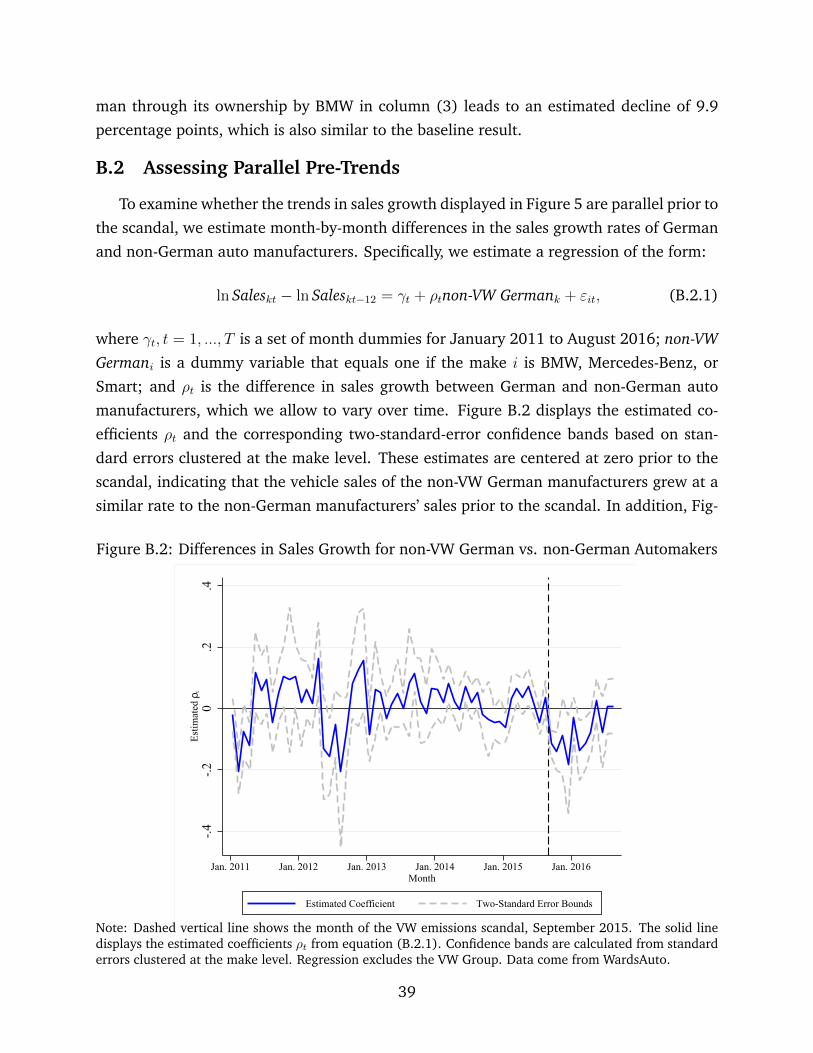
man through its ownership by BMW in column (3) leads to an estimated decline of 9.9

percentage points, which is also similar to the baseline result.

B.2 Assessing Parallel Pre-Trends

To examine whether the trends in sales growth displayed in Figure 5 are parallel prior to

the scandal, we estimate month-by-month differences in the sales growth rates of German

and non-German auto manufacturers. Specifically, we estimate a regression of the form:

ln Saleskt − ln Saleskt−12 = γt + ρtnon-VW Germank + εit, (B.2.1)

where γt, t = 1, ..., T is a set of month dummies for January 2011 to August 2016; non-VWGermani is a dummy variable that equals one if the make i is BMW, Mercedes-Benz, or

Smart; and ρt is the difference in sales growth between German and non-German auto

manufacturers, which we allow to vary over time. Figure B.2 displays the estimated co-

efficients ρt and the corresponding two-standard-error confidence bands based on stan-

dard errors clustered at the make level. These estimates are centered at zero prior to the

scandal, indicating that the vehicle sales of the non-VW German manufacturers grew at a

similar rate to the non-German manufacturers’ sales prior to the scandal. In addition, Fig-

Figure B.2: Differences in Sales Growth for non-VW German vs. non-German Automakers

-.4-.2

0.2

.4Es

timat

ed ρ

t

Jan. 2011 Jan. 2012 Jan. 2013 Jan. 2014 Jan. 2015 Jan. 2016Month

Estimated Coefficient Two-Standard Error Bounds

Note: Dashed vertical line shows the month of the VW emissions scandal, September 2015. The solid linedisplays the estimated coefficients ρt from equation (B.2.1). Confidence bands are calculated from standarderrors clustered at the make level. Regression excludes the VW Group. Data come from WardsAuto.

39

ure B.2 shows that, after the scandal, the sales of the non-VW German auto manufacturers

grew more slowly than the sales of the non-German auto manufacturers, consistent with

the difference-in-differences estimates in the main text.

B.3 Alternative Econometric Specifications

We show in this appendix that our difference-in-differences estimates are not sensitive

to alternative implementations. In Section 3.1, we weighted observations by the square

root of the make’s monthly sales volume. Column (2) of Table B.3 shows that our choice

to weight the observations is conservative: the unweighted estimate of the difference-

in-differences coefficient is 14 percentage points. In column (3), we consider mid-point

growth rates, where the change in sales volume between period t and period t − 12 is

divided by the average level of sales in the two periods. The estimated difference-in-

differences coefficient under this alternative measure is 9.4 percentage points, which is

similar to the baseline result in column (1).

Table B.3: Difference-in-Differences Estimates—Alternative Specifications

Dependent Variable 12-month Sales Growth

Specification Baseline Unweighted Mid-Point

(1) (2) (3)

German × Post-Scandal -0.092∗∗∗ -0.140∗∗ -0.094∗∗∗

(0.030) (0.058) (0.030)

Time Fixed Effects Yes Yes YesMake Fixed Effects Yes Yes YesR2 0.303 0.131 0.322N 2150 2150 2150

Note: Unit of observation is a make-month. Time period covered is January 2011 to August2016. Standard errors clustered at the make level in parentheses. VW Group (VW, Audi, andPorsche) excluded from all regressions. VW emissions scandal dated September 18, 2015. Salesare measured in units sold. Regressions in columns (1) and (3) are weighted by the square rootof sales volumes. Regressions in columns (1) and (2) use 12-month log sales growth as thedependent variable; column (3) uses mid-point sales growth. All regressions include make andtime fixed effects. Data come from WardsAuto. *** p < 0.01, ** p < 0.05, * p < 0.1.

40

C Additional Details on Demand Estimation & Simulations

In this appendix, we present additional details on the estimation of the model of ve-

hicle demand from Section 4. First, we provide summary statistics for the list prices and

vehicle characteristics used in the estimation. Second, we present the first-stage regression

results, in which we regress the endogenous variable, vehicle prices, on the instrumental

variables. Third, we present alternative decompositions of the three channels by which the

VW emissions scandal affected the vehicle sales of the other German auto manufacturers.

Fourth, we repeat the baseline simulations allowing for price adjustments.

C.1 Summary Statistics of Product Prices and Characteristics

Our estimation sample consists of 1,968 product-year combinations with sales of at

least 100 units, where a product is defined as a make-model-power type. Table C.1 reports

the summary statistics of list prices and product characteristics.

Table C.1: Summary Statistics of Product Prices and Characteristics

Mean Std. Dev. Min Max

Prices (2015-$1000) 36.31 20.87 9.90 202.43Horsepower/Weight 0.06 0.02 0.02 0.19Weight (1000 lb) 3.89 0.88 1.81 7.32Miles per Gallon 29.94 12.30 10.00 119.00Diesel 0.07 0.26 0 1Gas 0.79 0.40 0 1Other Power Type 0.13 0.34 0 1Germany 0.23 0.42 0 1Japan 0.33 0.47 0 1Korea 0.06 0.24 0 1United States 0.30 0.46 0 1Other Country 0.07 0.25 0 1

N 1,968Note: Unit of observation is a product-year. A product is defined as a make-model-power type(e.g., a Honda Civic with a gasoline engine). Time period covered is 2010 to 2016, with 2015omitted as the scandal year, just as in Table 2, which reports our demand estimates. Data comefrom WardsAuto.

41

C.2 First-Stage Regression

Table C.2: First-Stage Regression for Demand Estimation

Dependent Variable Price ($10,000)pjt

IV1 -0.005∗∗∗

(0.000)IV2 0.001∗∗∗

(0.000)IV3 -0.0006∗

(0.000)IV4 -0.0001∗∗∗

(0.000)ln Weight 5.350∗∗∗

(0.555)Horsepower/Weight (HP/1000lb) 0.982∗∗∗

(0.031)ln Miles-Per-Gallon 0.867∗∗∗

(0.196)VW Group × Post-Scandal 0.008

(0.209)Other German × Post-Scandal 0.541∗∗∗

(0.180)Diesel × Post-Scandal 0.402

(0.271)

Country Fixed Effects yesPower-Type Fixed Effects yes

Note: Excluded instrumental variables (IV1 – IV4) are the sum of product characteristics overclosely competing products. Let x(`)

jt denote the value of characteristic ` for product j at time t,

then IV` =∑

j′ 6=j 1(∣∣∣x(`)

j′t − x(`)jt

∣∣∣ < D`

)x

(`)j′t , where for ` = 1, 2, 3, 4 represents the horsepower,

weight, length, miles-per-gallon of product j, and D` is the standard deviation of attribute ` inthe data. Country Fixed Effects comprises indicators for German, Japanese, Korean, U.S., andAll Other country origins. Data come from WardsAuto. *** p < 0.01, ** p < 0.05, * p < 0.1.

42

C.3 Additional Simulations

In Section 4.3, we report three simulations in which we turn on the scandal’s three

channels sequentially in order to quantify the effect of each. There, the sequence in which

the channels are turning on is “Substitution Away from VW Group,” followed by “Sub-

stitution Away from Diesel,” and finally “Spillover to Other German Automakers.” That

sequence is, however, not unique: in fact, there are four quantifications of each channel’s

effect. Given the nonlinearity of the demand model, in principle these different quantifi-

cations can provide different answers regarding the magnitudes of each channel’s effect.

We can quantify the effect of each channel by comparing two scenarios: one in which the

channel is turned on, and one in which it is turned off. For each comparison, the other two

channels are either both turned on, both turned off, or one is turned on and one is turned

off. Table C.3.1 summarizes the simulation designs used in these four quantifications, and

Table C.3.2 reports the results (bold table entries correspond to the baseline quantification

in Table 4 in Section 4.3). As noted, the results turn out to be stable across these different

quantifications.

43

Table C.3.1: Simulation Designs

S1 S2 S3 Data S4 S5 S6 S7

# of Active Channels 3 2 1 0 2 2 1 1

Substitution Effect yes no no no yes yes yes no

Diesel Effect yes yes no no no yes no yes

Spillover Effect yes yes yes no yes no no no

Table C.3.2: Quantifications of Each Channel’s Effect on the non-VW German Automakers

Other Two Channels

On/On On/Off Off/Off

Substitution Effect S1 – S2 S4 – S3 S5 – S7 S6 – DataVehicle Sales 77,342 76,672 87,149 86,258Revenue ($ billion) 3.44 3.41 3.83 3.79

Diesel Effect S1 – S4 S2 – S3 S5 – S6 S7 – DataVehicle Sales 1,970 1,300 3,230 2,338Revenue ($ billion) 0.09 0.06 0.14 0.10

Spillover Effect S1 – S5 S2 – S7 S4 – S6 S3 – DataVehicle Sales –255,452 –245,645 –254,193 –244,607Revenue ($ billion) –11.67 –11.28 –11.62 –11.24

Note: Bold table entries correspond to the baseline decomposition in Table 4. Positive numbersindicate that the channel increased vehicle sales or revenue for the non-VW German automak-ers; negative numbers mean the opposite. The entries in the column titled “On/On” report thechannel’s effect in a simulation with the other two channels; e.g., the first row of that columnreports the effect of the substitution away from VW channel if the scandal had also led to sub-stitution away from diesel and a spillover to the other German automakers. The entries in thecolumns titled “On/Off” report the channel’s effect in a simulation with one of the other twochannels, as indicated by the simulation designs in Table C.3.1. Finally, the entries in the columntitled “Off/Off” report the channel’s effect in a simulation without the other two channels. Thesimulated effects are relative to 2014, the calendar year before the scandal. Revenue effects areexpressed in 2015 dollars.

44

C.4 Simulations with Price Adjustments

In the simulations in Section 4, we hold prices fixed in order to quantify how much each

individual channel of the VW emissions scandal shifts demand. We find that the spillover

effect is significant and is larger than the scandal’s net overall effect. In this section, we

show that these findings are robust to allowing for price adjustment.

To this end, we model the supply side of the U.S. light vehicle market, back out the

marginal cost of each product, and, in each simulation, compute the pricing equilibrium

based on these estimated marginal costs. We assume that firms compete in a Bertrand

fashion. Specifically, each firm k chooses the price of each of its products, denoted by Jkt,to maximize its profit:

maxpjt,j∈Jkt

∑j∈Jkt

(pjt −mcjt)sjt(pt), (C.4.1)

where the vectors pt capture the prices of all products in the market and the market share

function sjt(pt) is given by the demand model in Section 4. Non-price variables such as

product characteristics and demographics are absorbed in the subscript jt.

This profit-maximization problem implies the following first-order conditions:

sjt +∑j′∈Jkt

(pj′t −mcj′t)∂sj′t∂pjt

= 0 for any j ∈ Jkt, (C.4.2)

which can be rewritten in matrix form using the following notation. Let skt = (sjt, j ∈ Jkt)and define pkt and mckt analogously. Let #Jkt denote the number of products sold by

firm k in year t and ∇kt be a #Jkt-by-#Jkt matrix whose (j, j′) element is ∂sj′t∂pjt

. Then, the

first-order conditions in (C.4.2) can be rewritten as:

skt +∇kt(pkt −mckt) = 0. (C.4.3)

We can then solve for the marginal costs as:

mckt = pkt −∇−1kt skt, (C.4.4)

where market shares skt and prices pkt are observable, while the “slopes” of the market

share functions ∇kt are taken from the estimated demand model.

Based on these marginal costs, we repeat each simulation in Section 4 by first comput-

ing the Nash-Bertrand equilibrium prices with some or all of the scandal’s channels turned

on and then calculating the corresponding sales quantities and revenues. Table C.4 shows

that our key findings are robust to allowing for equilibrium price changes.

45

Table C.4: Scandal’s Impact on Other German Manufacturers with Price Adjustments

Comparison Vehicle Sales Revenue($ billion)

Overall Scandal Simulation 1 − Data –162,288 –7.57–22.98% –23.12%

Substitution Effect Simulation 1 − Simulation 2 81,004 3.6211.47% 11.06%

Diesel Effect Simulation 2 − Simulation 3 1,011 0.040.14% 0.11%

Spillover Effect Simulation 3 − Data –244,302 –11.22–34.59% –34.29%

Note: Simulation designs are defined in Table 3. Revenue effects are expressed in 2015 dollars.

46