Fire Sales and House Prices:

Evidence from Estate Sales due to Sudden Death*

Steffen Andersen Copenhagen Business School

Kasper Meisner Nielsen Hong Kong University of Science and Technology

January 2014

Abstract: This study investigates when forced sales turn into fire sales by using a natural experiment

which allows us to separate supply and demand effects: Forced sales result from sudden death of house

owners and are thus unrelated to current market conditions. We find that forced sales result in fire sale

discounts. Discounts increase when the sale is urgent, market conditions are poor, the seller is

financially constrained, or the seller exhibits the disposition effect. Overall, our study identifies when

forced sales lead to fire sale discounts, and highlights that fire sales occur even in the absence of

temporary demand shocks.

JEL Classifications: D14, R31

Keywords: Fire sales; Financial constraints; Real estate; Sudden death.

* We thank Rui Albuquerque, John Campbell, Sudipto Dasgupta, Mark Lane, Abhiroop Mukherjee, Tarun

Ramadorai, Rik Sen, Jared Stanfield, Dragon Tang, Ania Zalewska, and seminar participants at Aarhus University, American Real Estate Society 2013 Meeting, Australasian Banking and Finance Conference 2013, Boston University, Chinese University of Hong Kong, Copenhagen Business School, European Finance Association 2013 Meeting, Hong Kong Baptist University, Hong Kong University of Science and Technology, National University of Singapore, Nanyang Technological University, Paris School of Economics, University of Auckland, University of Bergen, and Victoria University for helpful comments and suggestions. We are grateful to the Danish Social Science Research Council for financial support through project 11-104456.

Corresponding author: Kasper Meisner Nielsen, Department of Finance, Hong Kong University of Science and Technology. Email: nielsen@ust.hk

1

1. Introduction

Forced sales of assets at fire sale discounts typically occur because of bankruptcy or financial

distress. Such sales are forced because the seller cannot satisfy an outstanding obligation without selling

assets, and the price is discounted because financial distress tends to be contagious within an industry

(Lang and Stulz, 1992). The highest potential bidder may therefore be facing financial constraints of

their own and be unable to buy the assets (Aghion, Hart, and Moore, 1992; Shleifer and Vishny, 1992,

2011). As a result, discounts on distressed assets are substantial. For instance, Pulvino (1998) shows

that used planes sold by distressed airlines bring 10% to 20% lower prices than planes sold by

unconstrained airlines.

Although prior literature has documented that fire sale discounts exist and can be substantial

(Pulvino, 1998; Coval and Stafford, 2007; Eckbo and Thorburn, 2008; Campbell, Giglio, and Pathak,

2011; Albuquerque and Schroth, 2012), it has been difficult to empirically identify when forced sales

result in fire sale discounts. Forced sales are typically triggered by industry-wide or asset specific adverse

shocks that affect both supply and demand for the asset. For instance, forced sales of distressed assets

typically become more urgent when asset prices fall, which makes it difficult to isolate the effect of

forced sales on prices from the effect of the confounding shock. Empirical identification of conditions

under which forced sales turn into fire sales therefore requires that one can separate supply and

demand effects.

This study investigates when forced sales turn into fire sales by using a natural experiment in

which a random asset independent of market conditions is forced to be sold over a short time horizon.

We exploit forced sales resulting from sudden deaths of house owners. The advantages of using sudden

deaths in our identification strategy are threefold. First, sudden deaths provide a close to random draw

of house owners which ensures that individual, as well as house, characteristics are exogenous to the

sample selection procedure. Second, forced sales due to sudden deaths are unrelated to current market

2

conditions and, thus, independent of the current supply and demand for the asset. This allows us to

identify market conditions under which forced sales occur at fire sale discounts. Third, estate sales are

forced to be resolved within 12 month because of the institutional environment. This allows us to

identify the urgency of the sale as the deadline nears.

Our identification strategy derives from the institutional setting surrounding inheritance cases in

Denmark. The Danish Inheritance Act of 1964 requires estates to be settled in probate court within 12

months after the death. As a result, the suddenly deceased’s house is either forced to be sold or forced

to be transferred to beneficiaries. Due to the institutional setting it is economically unattractive to

transfer ownership with the purpose of renting out or postponing the sale.1 As a result family transfers

mainly occur for non-pecuniary reasons; either because a beneficiary already lives in the house or

subsequently moves into house.2 More importantly transfers to beneficiaries are unrelated to current

market conditions and observable house characteristics, and only 7% of all family transfers are resold

within 2 years.3 Consequently, more than 90% of all houses in our sample end up being sold at arm’s

length, and the potential bias resulting from transfers of ownership within the family is likely to be

small due to the institutional setting.

Our empirical identification of estates relies on a conservative medical definition of sudden death

and unique cause-of-death data from official death certificates to identify 6,854 suddenly deceased

1 Transfers of ownership to beneficiaries can legally occur at a discount equivalent to 15% of market value of the house. Thus, the tax benefit of transferring ownership to beneficiaries equals 2.25% of the house value (= 15% discount on the price multiplied by the 15% estate tax). The net benefit is low, and in many cases negative, because of transaction costs, foregone cash flows, yearly property taxes, agency costs due to rent control, limited contractual freedom, and restrictive planning and zoning laws that require that houses in Denmark either are occupied or for sale. For instance, changes to the land register are subject to a fee equivalent to DKK 1,400 (EUR 187) plus 0.6% of the house value. Most property purchases are financed by mortgages, which are subject to a mortgage deed stamp equivalent to 1.5% of the face value. Facilitation of the transfer of ownership requires legal assistance, which on average costs around DKK 8,000 (EUR 1,070). Finally, properties are subject to a yearly property tax (at least 1% of the property value) and municipality land tax (varies between 0.06% and 0.24% of the value of the lot). 2 In almost half of the family transfers a beneficiary lived in the house prior to death, and in 83% of the family transfers a beneficiary lives in the house after the family transfer. 3 In the online appendix we show that transfers of ownership to beneficiaries are unrelated to the house price growth and observable house characteristics. In addition we find no difference in the tax authorities’ assessment of house value (prior to death) between houses that are transferred to beneficiaries or sold, respectively.

3

house owners during the period from 1992 to 2009. We identify the first transaction of the house

following the death and focus exclusively on arm’s-length transactions in which the buyer is unrelated

to the deceased or the beneficiaries. We do so because transfers within the family are likely to occur at

discounted prices to minimize the estate tax. Our sample of forced sales therefore consists of 6,329

arm’s-length transactions, which corresponds to 0.7% out of a total of 877,559 house sales in the

period from 1992 to 2010.

To examine the effect of forced sales we follow a standard approach in real estate economics: we

regress the logarithm of the house price on house characteristics, calendar month indicators, and

municipality-year fixed effects. We find that forced sales result in an average discount of 6.6%. The

discount is increasing as the deadline nears. Sales shortly after the sudden death occur at market prices,

while sales in the last three months before the deadline result in an average discount of 12.5%.

Although asking prices might decline with the time on the market, the pricing pattern suggests that time

on the market cannot alone explain the estimated discount. Under the alternative hypothesis of a time

on the market effect, one would expect to observe a premium on early forced sales and a discount on

late forced sales because we benchmark to realized prices for average time on the market. We observe,

on the contrary, that early sales occur at market prices and late sales occur at deep discounts. In

addition, Genesove and Mayer (1997) and Levitt and Syverson (2008) provide evidence that sellers who

keep their houses on the market longer realize higher prices.

Having established that forced sales result in discounts, we examine how market conditions affect

the discount. We expect larger discounts when market conditions are poor because forced sales do not

have the option of withdrawing the house from the market. We find an average discount of 5.5%

during quarters when prices increased by 2.5% or more, while the discount during quarters when house

prices contract averages 9.9%. Thus, the discount is 4.4% larger during quarters with contracting house

prices (busts), consistent with theoretical predictions in Shleifer and Vishny (1992), where discounts

result from negative industry-wide shocks. We further examine whether discounts are affected by local

4

market conditions. To capture local demand, we both count the number of sales within each

municipality in each year and calculate the local market turnover as the number of sales divided by the

number of houses in each municipality in each year. We find larger discounts in areas with fewer sales,

and a small discount in the most active local markets. More importantly, our findings of discounts

during booms and in active local markets highlight that discounts arise when sales are urgent even in

the absence of an adverse shock affecting the demand for the asset.

To understand the importance of the financial position of the seller in determining the forced sale

discount, we identify financially constrained estates and beneficiaries for whom alternatives to selling

are limited. In our setting the seller’s financial position is exogenous to the forced sale because the sale

is triggered by the sudden death. We can therefore empirically identify the effect of financial constraints

on fire sale discounts. We classify estates as financially constrained if their net wealth excluding house

equity is negative. These estates all have positive net wealth, but the wealth is tied in the house. To meet

liabilities and incur the estate tax the house therefore needs to be sold. As expected, forced sales of

houses by financially constrained estates occur at an incremental discount of 7.7% relative to other

forced sales. We also identify estates with less than DKK 50,000 in financial wealth (value of bank

deposit, stocks, and bonds) as liquidity constrained and find an incremental discount of similar

magnitude. The time pattern of discounts for sales by financially constrained estates reveals substantial

discounts of 5% to 10% for early sales, while sales shortly before the deadline occur at discounts of

15% to 25% for liquidity constrained estates. Financial constraints are, thus, an important determinant

of fire sale discounts.

One concern with our results is that discounts might be driven by unobserved heterogeneity in

the quality of houses. Although sudden deaths provide a close to random draw of houses and their

owners, which limits concerns about unobserved heterogeneity (Campbell, Giglio, and Pathak, 2011),

we further examine two subsamples for which such concerns are limited. The first subsample excludes

sudden deaths of individuals aged 65 or above from our analysis, because quality and maintenance are

5

expected to decline with owner age. The second subsample focuses exclusively on forced sales of

houses owned by individuals who died in a traffic accident. With the latter subsample, the assumption

about a random draw of property owners is more likely to be satisfied. This subsample also rules out

concerns about whether discounts relate to superstition, as traffic accidents, by definition, occur outside

the deceased’s house. For both subsamples, we find discounts of similar magnitude. Finally, we note

that the time pattern of discounts and the magnitude of the discounts also make it implausible that the

discounts are related to poor quality or lack of maintenance.

Another concern relates to our ability to price houses using hedonic regressions. To overcome

this issue we rely on the Danish Tax and Customs Administration’s assessment of property values,

which forms the basis for the annual property tax. The assessment is an estimate of the property’s cash

price if it were to be sold. The assessment is carried out by the local tax authorities and takes into

account a wide array of house characteristics as well as local market conditions. The assessed value

appears to be a valid estimate of house prices, as the average difference between assessed values and

realized prices is 3.1%. Moreover, it seems reasonable to argue that the assessed house value is unbiased

in relation to sudden deaths. This allows us to estimate the forced sale discount using a difference-in-

differences estimate that compares the difference between the realized price and the assessed value

between forced sales and non-forced sales. The difference-in-differences estimate of the forced sale

discount equals 9.7%, which is larger than the estimated discount of 6.6% obtained from the hedonic

regression model.

Our results raise the question of whether estate sales are optimally conducted or, alternatively,

beneficiaries are making mistakes. Discounts might occur as a result either of an optimal sales strategy

that has encountered bad luck or of beneficiaries setting prices that deviate from market prices. We

note that bad luck cannot alone explain discounts: Late fire sales are more likely when the house price

is in the loss domain suggesting that disposition effects might play a role in explaining discounts. While

either explanation will result in the observed time pattern of discounts, we note the occurrence of

6

substantial discounts for early sales by financially constrained beneficiaries and estates. These results

suggest that discounts are high when sales are urgent because sellers cannot satisfy outstanding

obligations without selling the asset.

Collectively, our results show when forced sales result in fire sale discounts. Overall, the results

are consistent with the theoretical predictions of Shleifer and Vishny (1992). Discounts are determined

by the urgency of the sale, market conditions, and the financial position of the seller. Perhaps more

surprisingly we find evidence of discounts, although small, during booms and in the most active local

property markets. These findings suggest that discounts arise when sales are urgent even when potential

buyers are unaffected by the event forcing the sale. These results are consistent with Albuquerque and

Schroth (2012), who model asset sales by use of a search model. Search frictions in the housing market

result in fire sale discounts when sellers are forced to find buyers over short time horizons.

The closest empirical analysis to our study is Campbell, Giglio, and Pathak (2011), who show that

forced sales of houses occur at discounts. They consider three types of forced sales related to

bankruptcy, death, and foreclosure. For bankruptcy-related sales, the average discount is 3%, followed

by, for deaths, 5%-7%, and, for foreclosures, 27%. In contrast to Campbell, Giglio, and Pathak (2011),

we focus on forced sales due to sudden death because it provides us with a close to random draw of

house owners which ensures that forced sales are unrelated to current market conditions and limits

concerns about unobserved heterogeneity. Campbell, Giglio, and Pathak (2011) provide evidence of

substantial discounts for forced sales of houses, but cannot separate supply and demand effects, which

is necessary to empirically identify when forced sales turn into fire sales. Our approach allows us to

convincingly identify market conditions and constraints under which forced sales lead to fire sale

discounts.

Understanding the conditions under which forced sales lead to fire sale discounts is important

because fire sales and efforts to avoid them have implications for a wide range of financial and

economic outcomes. For instance, fire sales affect the structure and terms of debt contracts (Shleifer

7

and Visnhy, 1992; Benmelech, Garmaise, and Moskowitz, 2005; Benmelech and Bergman, 2009, 2011;

Ortiz-Molina and Phillips, 2010). Fire sales might also have spillover effects that can lead to downward

spirals or cascades in asset prices and net worth of market participants (Kiyotaki and Moore, 1997;

Gromb and Vayanos, 2002; Coval and Stafford, 2007; Campbell, Giglio, and Pathak, 2011) and

creditors (Acharya, Bharath, and Srinivasan, 2007), resulting in real effects through reduced investment

and output (Kiyotaki and Moore, 1997; Ivashina and Scharfstein, 2010; and Shleifer and Vishny, 2010).

In relation to these important issues, our results provide new insights about when forced sales are likely

to result in costly fire sales.

Section 2 outlines empirical strategy, presents our data, and provides summary statistics. Section 3

presents the results, while Section 4 considers alternative specifications. Section 5 concludes.

2. Estate sales due to sudden death

We assemble a unique dataset from Denmark that allows us to identify house owners who

suddenly die and to subsequently follow the sale of their houses by the estate. In addition to supplying

micro-data from administrative registers, the Danish case also provides us with a legal environment in

which estates have to be settled within 12 months following the death. The probate court will only in

rare cases extend the liquidation period beyond 12 months.4 As the deadline nears, the probate court

will schedule a meeting to finally settle the estate. This meeting legally has to occur, at the latest, 3

months after the end of the liquidation period and, hence, 15 months after the death. If the deceased’s

house is not sold at this point, the probate court may order the house to be auctioned off.

We focus exclusively on estates where all beneficiaries are offspring (i.e., where the suddenly

deceased was a widow or widower, or in rare cases, a couple). This focus simplifies the analysis, as

4 In more involved estates, a lawyer may be appointed to resolve the estate on behalf of the deceased and the beneficiaries. In such cases, the legal deadline for settlement of the estate is 24 months. Lawyers are, according to the Ministry of Finance (1999), appointed to 8.4% of all estates, and this typically occurs whenever disputes exist among beneficiaries.

8

children, according to the Danish Inheritance Law of 1964, will inherit by default the estate in

proportional shares in all such cases.5 The net worth of such estates is subject to a 15% estate tax for

offspring if it exceeds DKK 191,000 (EUR 25,638) in 1998. This threshold is inflated by a price index

in subsequent years.

Identification of estates is facilitated by the institutional environment. Danish law requires that a

death certificate be issued by a doctor when a citizen dies. If the person dies at home, the death

certificate is filled out by the personal doctor or the emergency doctor on duty (Lægevagten). If the

person dies in the hospital, a doctor at the hospital will issue the death certificate. The death certificate

classifies the cause of death according to guidelines established by the World Health Organization.

Danish law further obliges the relatives to report the death to their local funeral authority within

two days. The funeral authority formally notifies relevant government agencies, including the Central

Office for Personal Registration (CPR Registeret) and the probate court (Skifteretten), which supervises

the process that transfers legal title of property from the decedent’s estate to her beneficiaries. The

probate court immediately seizes the decedent’s assets, with the purpose of meeting liabilities and

settling the estate. The probate court posts a notice in The Danish Gazette (Statstidende) to advertise for

creditors, who in turn have 8 weeks to report their claims on the estate. Following the notice period,

assets are either liquidated or valued by the probate court with the purpose of establishing the net

worth of the estate, meeting liabilities, and incurring the estate tax. At the closing of the estate, the

residual is paid out to the beneficiaries. According to the Association of Danish Estate Lawyers, it

takes, on average, 9 months to resolve an estate.

5 The default sharing rules can only partially be offset by the existence of a will that, by Danish law, must be publicly available before the death. Although opting out through wills is possible in Denmark, the inheritance law ensures that children will inherit at least 50% of the estate in the cases we consider. Moreover, opting out of the default sharing rule is extremely rare, as only 2% of the empirically relevant individuals in Denmark have drafted a will (Ret og Råd 2008).

9

A. Data sources

Our data cover the universe of adult Danes in the period between 1990 and 2010. Our dataset

contains economic, financial, and personal information about decedents and beneficiaries. We derive

data from five different sources made available through Statistics Denmark; the sources are:

1. Causes of deaths from the Danish Cause-of-Death Register at the Danish National Board of

Health (Sundhedsstyrelsen). This dataset classifies the cause of death accordingly to international

guidelines specified by the World Health Organization’s International Classification of Diseases

System.6 Before 1994, diseases are classified using ICD-8 codes, and from 1994 and onward, using

ICD-10 codes. The source of these data is the official death certificates that are issued by a doctor

immediately after the death and convey a medically qualified opinion on the cause of death. The Danish

National Board of Health compiles these data for statistical purposes and makes it available for medical

and social science research through Statistics Denmark. We have obtained the cause of death for all

Danish citizens who passed away between 1992 and 2009.

2. House transactions are from the Danish Tax and Customs Administration (SKAT). SKAT

receives the information from The Danish Gazette (Statstidende). Public announcement in The Danish

Gazette is part of the juridical registration of the transfer of ownership, which ensures that we have

access to accurate and reliable information on prices of house transactions over the sample period.

3. Individual characteristics of houses are from the Housing Register (Bygnings- og Boligregister,

BBR). The Housing Register has detailed information on the individual characteristics of all houses in

Denmark. The information is available at the end of each year, and year-to-year changes are supplied by

municipalities based on planning permissions. According to Danish law, house owners are obliged to

apply for planning permission before undertaking any significant alteration of their property. From this

dataset, we obtain individual characteristics of all houses in Denmark: interior size, lot size, 6 WHO’s International Classification of Diseases, ICD-10, is the latest in a series that has its origin in the 1850s. WHO took over the responsibility of ICD at its creation in 1948, and the system is currently used for mortality and morbidity statistics by all Member States. The ICD-10 standard replaced the ICD-8 standard in 1994.

10

construction year, bathrooms, and basement size. We use this data to explain variations in house prices

related to house characteristics.

4. Individual and family data from the official Danish Civil Registration System (CPR Registeret).

These records include the individual’s personal identification number (CPR numbers); name; gender; date

of birth; CPR numbers of nuclear family members (parents, siblings, and children); and the individual’s

marital history (number of marriages, divorces, and widowhoods). We use these data to identify all

individuals’ legal parents. The sample contains the entire Danish population and provides a unique

identifying number across individuals, households, and time.

5. Income and wealth information from the official records at the Danish Tax and Customs

Administration (SKAT). This dataset contains total and disaggregated income and wealth information

by CPR numbers for the entire Danish population. The tax authorities receive this information directly

from the relevant sources: employers supply statements of wages paid to their employees. Financial

institutions supply information on their customers’ deposits, interest paid (or received), security

investments, and dividends. Because taxation in Denmark mainly occurs at the source level, the income

and wealth information are highly reliable. The data from the tax authorities also contain an assessment

of house values, which forms the basis for the property value tax and the municipality land tax.7 The

assessment is carried out every other year, and is an estimate of the property’s cash price if it were to be

sold. The valuation takes into account factors such as local market conditions, an array of house

characteristics, and permissible alternative uses of the land. In years in which a house is not assessed by

the tax authorities, the value is regulated based on the growth in local house prices in the period

following the most recent assessment. As the assessment is carried out at the municipality level, it might

incorporate factors that are unobserved in the data from the Housing Register. The assessment of

house values by the tax authorities therefore provides us with a house-specific estimate of the expected

7 House owners pay a progressive annual property tax starting at 1% of the assessed property value, and an annual municipality land tax varying between 0.06% and 0.24% of the assessed value of the lot.

11

price. Through Statistics Denmark, we have obtained access to data on income, wealth, and house

valuations from 1990 to 2010.

Taken together, these data sources allow us to identify forced sales of houses, examine whether

forced sales result in lower prices relative to comparable houses, and characterize market conditions

under which forced sales lead to fire sale discounts.

B. Data construction

To identify forced sales, we link the data on deceased individuals to the data on house ownership

and sale of houses. We focus on the house market as the markets for cottages, apartments, and

condominiums in Denmark are geographically clustered and cater to specific socio-economic groups.

The house market, on the other hand, is significantly larger, covers all geographic locations, and has

widespread participation by most segments of the population.

The starting point of our analysis is to identify estates. In total, we identify 208,283 estates

between 1992 and 2009. Table 1 shows the individual characteristics of the decedents and their estates.

Among these estates, we identify the cause of death with the purpose of selecting a sample of estates

resulting from sudden and unexpected death. To identify sudden and unexpected deaths, we follow

Andersen and Nielsen (2011, 2012), who identify relevant ICD-10 codes from related medical literature

combined with a thorough inspection of WHO’s detailed classification system.8 Thus, among natural

deaths, we consider acute myocardial infarction (ICD-10: I21-I22), cardiac arrest (I46), congestive heart

failure (I50), stroke (I60-I69), and sudden deaths by unknown causes (R95-R98) as sudden deaths.

Among unnatural deaths, we classify traffic accidents (V00-V89) and other accidents and violence

8 See WHO’s webpage at www.who.int/classifications/icd/en, and Andersen and Nielsen (2011) for references to the medical literature. The ICD-10 classification system was introduced in 1994. Thus, for 1992 and 1993 we rely on the ICD-8 classification system. Corresponding ICD-8 codes are: acute myocardial infarction (4101-9); cardiac arrest (4272); congestive heart failure (4270-1, 4273); stroke (430-8), sudden deaths by unknown causes (795-6); traffic accidents (800-827); and other accidents and violence (830-849, 870-929).

12

(V90-V99, X00-X59, and X86-X90) unanticipated by the relatives as sudden deaths. According to this

definition, 48,938 of the estates result from sudden deaths.

Among estates resulting from sudden death, we identify 6,854 estates with 7,022 houses that are

forced to be sold. The final step in our sample selection entails determining whether sales occur at

arm’s length because transfers within the family are likely to occur at discounted prices to minimize the

estate tax. Out of 7,022 houses, ownership is transferred to a beneficiary in 693 cases. In 311 (45%) of

these cases a beneficiary already lived in the house before the death event, and in 572 of the family

transfers (83%) a beneficiary subsequently lives in the house. The remaining 121 (17%) transfers within

the family are subsequently rented out. In the online appendix we examine the propensity to transfer

ownership within the family and find that it is unrelated to current market conditions and observable

house characteristics. We also note that few of these transfers subsequently are resold. Only 49 out of

693 (7%) transfers of ownership within the family are resold after 2 years. We conclude that family

transfers appear to occur for non-pecuniary reasons and that the potential bias resulting from transfers

of ownership within the family is likely to be small due to the institutional setting. In the following we

focus exclusively on arm’s lengths transactions. Our final sample therefore includes 6,181 estates with

6,329 houses where the beneficiaries are forced to sell the house to settle the estate.

In our final sample, the deceased has net wealth of DKK 987,200 (EUR 132,500), of which

property wealth contributes the majority. The deceased in the forced sale sample has significantly

higher property wealth and net wealth than all estates that result from sudden death because we

condition on house ownership. We also note that despite our use of a medical definition of sudden

deaths, the decedents in our sample are 74.2 years old, which spurs concerns about whether our

analysis will be confounded by unobserved house characteristics such as maintenance. In the empirical

analysis, we address this concern by focusing on i) decedents younger than 65, ii) traffic accidents, and

iii) use of propensity score matching on the seller’s age.

13

Table 2 presents summary statistics for all house sales as well as our final sample of forced sales

from 1992 to 2010. In total, our data include 877,559 house sales, of which 6,329 (0.7%) are classified

as forced. Panel A reports individual characteristics of houses. The average house has an internal size of

128.2 square meters (excluding basement), has a lot of 879.3 square meters, and is 50.9 years old. One

out of three houses has a basement, and the average size of basements is 31.5 square meters. In

comparison, forced sale houses have smaller interior size and lots, and are slightly older.

Panel B of Table 2 shows the geographic distribution of house sales. Although forced sales

appear to be geographically diverse, and close to the distribution of non-forced sales, the distributions

are statistically different. This difference is explained by the fact that forced sales reflect the distribution

of the population, while non-forced sales reflect the activeness of the local property market. The house

market is more active in the Capital region and, as a result, forced sales are slightly underrepresented in

this region. In the empirical analysis, geographic location is based on municipalities. From 1992 to

2002, Denmark was subdivided into 275 municipalities. A series of municipality reforms reduced the

number to 271 in 2003, to 270 in 2006, and finally to 98 in 2007.9

Panel C shows the seasonal distribution of house sales. The housing market tends to be more

active in the second quarter and less active in the fourth quarter. This tendency is hardly surprising

given Denmark’s location in the northern part of the Northern Hemisphere, which results in

significantly longer (shorter) days during summer (winter).

Finally, Panel D reports the average house price as well as the tax authorities’ assessment of the

value prior to the transaction. The average house price over the sample period equals DKK 1,091,800

(EUR 146,500). In comparison, forced sales occur at lower prices. The average price of a forced sale is

DKK 959,500 (EUR 128,800). While the differences in house characteristics collectively suggest that

9 From 1992 to 2002, our data include 275 municipalities. In 2003, the five municipalities on the island Bornholm merged, which reduced the number of municipalities to 271. In 2006, two municipalities on the island Ærø merged, which reduced the number of municipalities to 270. In 2007, a municipality reform reduced the number of municipalities to 98.

14

houses owned by the suddenly deceased should be priced lower, the tax authorities’ assessment of the

value suggests that individual characteristics only account for a small fraction of the difference in price.

The tax authorities’ assessment of value (prior to the sale) suggests that forced sales result in large

discounts. The average assessed house value for forced sales is DKK 1,099,300, compared to DKK

1,126,000 for non-forced sales. If the assessed value provides an unbiased estimate of the value, we can

estimate the discount on forced sales as the difference between the house price and the assessed house

value relative to non-forced sales. For forced sales, the discount is equivalent to DKK 139,800 (12.7%),

whereas other sales occur at prices that are DKK 33,300 (3.0%) lower than the assessed value. This

yields a difference of DKK 106,500 (9.7%), which is statistically significant at the 1% level. Thus, by

using the tax authorities’ assessment of value prior to the transaction as benchmark, we obtain a 9.7%

difference-in-differences estimate of the forced sale discount.

3. Empirical results

A. A model of house prices

We follow Campbell, Giglio, and Pathak (2011) and estimate the relationship between the price

of houses and their characteristics using a hedonic regression, which is a standard approach in real

estate economics. The main equation for estimating the forced sale discount is specified in Equation

(1), where the dependent variable is the log price, yijt , of house i in municipality j in year t:

���� = ��� + �′� + �′�� + ���, (1)

where αjt captures municipality-year fixed-effects, Xi is a vector of house characteristics, and Fi is

an indicator for forced sales. House characteristics include: interior size (square meters), lot size (square

meters), basement indicator, basement size (square meters), number of bathrooms, house age, house

age squared, and calendar month indicators.

15

Table 3 reports our estimates of the coefficient of house characteristics, β, and the forced sale

discount, γ. We note that the coefficients on house characteristics all have the expected sign and

plausible magnitudes. In Column 1, we find an estimated coefficient for the indicator for forced sales of

-0.0681, corresponding to a price discount of 1-exp(-0.0681) = 6.6%.

Column 2 in Table 3 estimates the price discount conditional on the time of sale relative to the

death. If the estimated discount is related to the sale being forced by the provisions in the inheritance

law, we expect the discount to be larger for sales that occur close to the 12-month deadline. In Column

2, we therefore include an interaction term between the indicator for forced sale and the number of

months that have passed after the death. We notice that the discount is increasing as the time to the

deadline nears. The discount increases by 0.8% per month, implying that sales that occur right after the

death have a small discount, whereas sales shortly before the deadline are priced around 10.7% lower

than comparable houses.10

In Column 3, we examine whether the discount is increasing as the time to the deadline nears.

We include four indicators for forced sales depending on the time lag between the death and the sale.

Again, we find a much larger discount for sales that occur close to the deadline. Forced sales occurring

0-90 days (0-3 months) after the death are sold at prices identical to comparable houses. Forces sales

after 91 to 180 days (3-6 months) and 181-270 days (6-9 months) have an average discount of 5.8% and

10.5%, respectively. Forced sales after 271 days (9+ months), and hence shortly before the deadline,

occur at a 12.5% discount. Urgent sales lower prices, which is consistent with Mayer (1995, 1998), who

studies the effect of urgent sales on prices in real estate auctions.

As mentioned in Section 2, it is possible that some sales occur more than 12 months after the

death. The deadline can be extended if i) a lawyer is appointed to resolve the estate due to family

disputes; ii) the probate court orders the house to be liquidated at an auction; or iii) a sale is being 10 The discount after 12 months is calculated as the sum of the coefficients on the forced sales indicator and the coefficient on the interaction term between forced sale and month after death: (1-exp(-0.0192)) + (1-exp(12*-0.0077) = 10.7%.

16

negotiated.11 Out of 6,329 forced sales in our sample, 728 (11.5%) are sold more than 12 months after

the death. Of these 728 sales, more than 65% are sold in the following 6 months (i.e., 12 to 18 months

after the death). Only 85 (1.3%) sales occur more than 24 months after the death. In unreported

regression, we have extended the specification in Column 3 of Table 3 to differentiate between the

timing of sales after 9 months. Sales after 9 to 12, 12 to 15, 15 to 18, and 18+ months occur at

discounts of 11.0%, 11.0%, 15.5%, and 16.5%, respectively. In comparison, the estimates in Column 3

of Table 3 for sales after 6 to 9, and after 9+ months, yield discounts of 10.5% and 12.5%, respectively.

The pricing pattern suggests that time on the market cannot alone explain the estimated discount.

If sellers gradually lower their asking prices over time, our hedonic pricing model will price houses

relative to the average time on the market. If time on the market is driving the estimated time pattern,

one would expect to observe a premium on early forced sales and a discount on late forced sales. We

observe, on the contrary, that early sales occur at market prices and late sales occur at deep discounts.

Overall, the time pattern in columns 2 and 3 of Table 3 shows that discounts increase as the deadline

nears: forced sales close to deadlines occur at fire sale discounts.

B. The effect of market conditions on the forced sale discount

In the theoretical model by Shleifer and Vishny (1992), discounts occur because the industry

buyers, who are the most natural candidates for buying the asset, might themselves be financially

constrained and, hence, unable to bid when the assets are being liquidated. Thus, it is natural to

hypothesize that market conditions will affect the discount because forced sales do not have the option

of withdrawing the house from the market. Liquidation in markets during periods with low demand

should result in larger discounts, whereas the discount should be smaller in active markets. Because

11 Formally, beneficiaries have 3 months to report the final outcome of the liquidation of the estate to the probate court. This practice stretches the deadline to 15 months if the beneficiaries can manage to schedule the appointment with the probate court at the last possible day.

17

forced sales in our sample are exogenous to market conditions, we can directly identify the interaction

between forced sale discounts and market conditions. Table 4 reports the results.

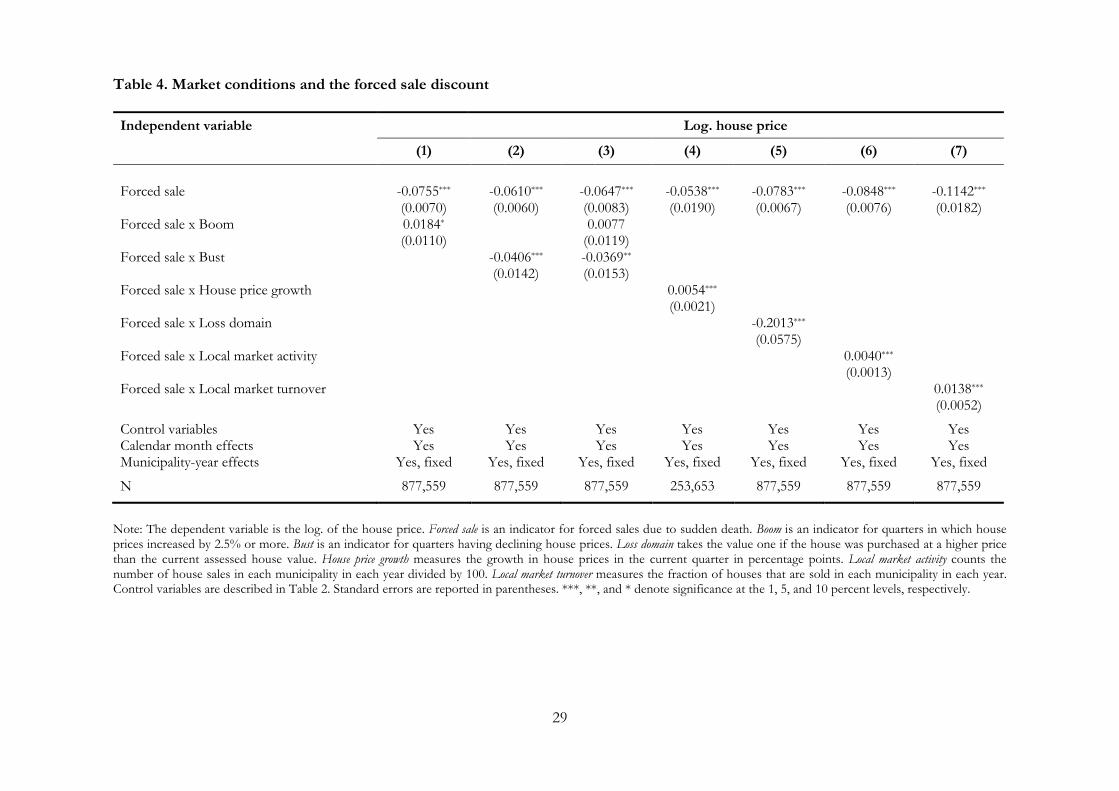
In columns 1, 2, and 3, we examine the magnitude of the forced sale discount during booms and

busts. Booms are defined as quarters during which house prices increased by more than 2.5%. Busts are

defined as quarters having declining house prices. In Column 1, we find that discounts are 1.9% lower

during booms, and in Column 2, we find a 4.0% higher discount during busts. When we include the

boom and bust effects together in Column 3, we find an average discount during booms of 5.5%, while

the discount during busts averages 9.9%. Thus, discounts are 4.4% larger in busts than in booms. In

Column 4, we interact the house price growth in each quarter with the forced sale indicator. Again, we

find larger discounts when house prices are declining.

The large discounts in busts beg the question whether the disposition effects plays a role. If so,

sales at high discounts are more likely if the house was purchased above the current market value

because beneficiaries will be reluctant to sell at current prices. We therefore restrict the sample to

houses that were purchased after 1992 and sold again in the period between 1992 and 2010. As a result

the sample is reduced to 253,653 house sales of which 740 are forced. To capture the reluctance to sell

at realistic prices we construct an indicator for houses that are in the loss domain. Houses are in the

loss domain whenever the house was purchased at a price above the current assessment of value by the

tax authorities. In total 101 out of 740 forced sales in this subsample are classified as being in the loss

domain. Column 5 in Table 4 reports the results. We find an average discount of 5.2%, and an

incremental discount of 18.2% for forced sales of houses in the loss domain. This suggests that the

disposition effect play an important role in explaining fire sale discounts.

In Column 6 of Table 4, we examine the interaction between the local market activity and the

forced sale discount. We use the total number of house sales in each municipality each year (divided by

100) to measure the level of local housing market activity. Any direct effect of market activity on prices

is captured by the municipality-year fixed effect. Column 6 in Table 4 shows that the discount is larger

18

in thin markets. In areas with few house sales per year, the average discount on forced sales equals

7.5%. As the local market becomes more active, the discount declines. The most active local market has

around 950 house sales per year (thus, market activity = 9.5); here, the forced sale discount equals

2.3%. In Column 7, we interact the forced sale indicator with the local market turnover, which is

defined as the number of sales over the number of houses in each municipality in each year measured

in percentage points. Again we find smaller discounts in more active local markets, whereas discounts

are larger in thin local markets. Using market turnover to measure market conditions the discount

ranges from 2.1% to 10.0% from the most to the least active local market.

The market for houses is dominated by families whose sizes range from 2 to 4, which results in a

larger demand for houses with an interior size that caters to this segment. As a result, the demand for

small houses is thinner than the demand for medium-sized houses. Similarly, large houses cater to large

families or wealthy families that can afford the extra space. If the forced sale discount is driven by thin

demand, we expect the discounts on small and large houses to be larger than the discount on medium-

sized houses. We therefore interact the forced sale indicator with indicators for each decile of the

distribution of interior size. The lowest decile consists of houses with an interior size of less than 82

square meters, whereas houses in the largest deciles have an interior size of at least 180 square meters.

Figure 1 summarizes the estimated forced sale discount across the distribution of house sizes.

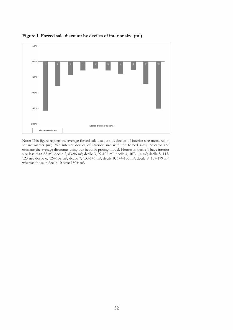
Figure 1 shows larger discounts at the lowest decile. For the smallest houses in decile 1, the

discount equals 15.7%. The discount gradually declines as we move toward the middle of the

distribution of interior size, and, for houses of median size in decile 5 and 6, the average discount

equals 2.6%. As the interior size gets beyond the median, the forced sale discount again starts to

increase. In the largest size decile, the discount equals 15.1%. The pattern in Figure 1 further bolsters

our identification strategy because it is hard to reconcile the pattern with concerns about maintenance

or unobserved house characteristics. Because the cost of maintenance is increasing in size, lack of

19

maintenance cannot explain why small houses are sold at the largest discount. Overall, the pattern in

Figure 1 is consistent with the hypothesis that the discount increases if the demand is thin.

C. The effect of financial constraints on the forced sale discount

Prior studies of forced sales (e.g., Pulvino 1998; Eckbo and Thorburn, 2008; Campbell, Giglio, and

Pathak, 2011) show that discounts are large when the seller is financially distressed. In our setting,

forced sales are unrelated to the financial conditions of the seller and the state of the economy, which

allows us to separate the effect of financial constraints from market conditions. From 1996 and

onward, our data include information about the financial position of estates and beneficiaries. The

financial position of the estate is important because it impacts the estate’s ability to pay ongoing

expenses like property taxes and utility bills. If the net wealth of the estate is tied in the house, the

ability to pay such expenses is limited, and the liquidity need might force the beneficiaries to sell the

house earlier at a lower price. The financial position of the estate also affects the beneficiaries’ ability to

incur the 15% estate tax without selling the house. While we stress the importance of financial and

liquidity constraints it should be noted that the estates in our sample generally have significant wealth

(see Table 1) providing them with sufficient means to maintain the house. Our measures of financial

constraints are therefore likely to be unrelated to the quality of houses prior to the deaths.

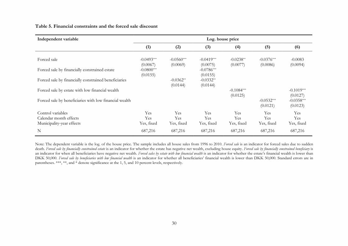
Our first measure of financial constraints in an indicator for estates with negative non-housing

wealth. Due to the availability of data on financial positions, we restrict the sample to house sales

between 1996 and 2010. Out of the 5,324 forced sales in this period, 1,001 (18.8%) of the estates are

financially constrained according to our measure. Column 1 in Table 5 estimates the forced sale

discount for such estates. We find a general discount of 4.8%, and an additional discount of 7.7% for

forced sales by financially constrained estates. Thus, houses sold by constrained estates are priced

12.5% below comparable houses. In Column 2, we examine the effect of financially constrained

beneficiaries on the discount. We find a negative incremental discount of 3.6% whenever all the

20

beneficiaries are financially constrained. In Column 3, we include both effects and note that discounts

are driven by sales by both financially constrained estates and beneficiaries.

Our second measure of financial constraints captures estates with little financial wealth. We

construct an indicator variable for estates holding less than DKK 50,000 of financial wealth (the sum of

bank deposits, stock, and bonds). According to this measure, 1,993 of the 5,324 (37.4%) estates are

likely to face a liquidity pressure to sell. Again, we interact the indicator for low financial wealth with

the indicator for forced sales. Column 4 in Table 5 reports the results. We find a large discount for

estates with low financial wealth, as the incremental discount equals 10.3%. In Column 5, we similarly

find larger discounts when all beneficiaries have low financial wealth. The incremental effect of the

discount is 5.2%. In Column 6, we include both effects, and again we note that discounts are driven by

the financial position of both the estate and the beneficiaries.

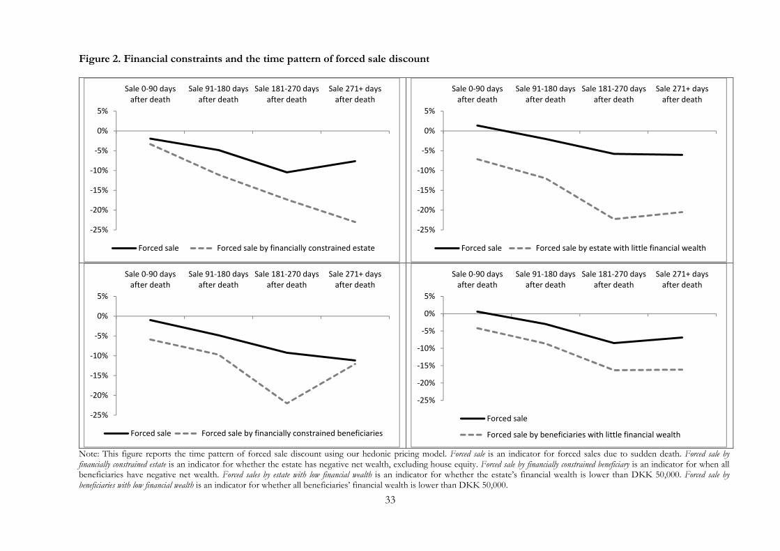
In Figure 2, we examine the time pattern of the forced sale discount for financially constrained or

liquidity constrained estates. If estates or beneficiaries are financially constrained or liquidity

constrained, it is likely that they will sell earlier by lowering the asking price. If so, we expect to find an

even larger effect of financial constraints on the price once we control for the timing of the sales

relative to the deadline. To examine the time pattern, we estimate the hedonic pricing model with

indicators for the timing of the sale and interactions between these timing indicators and financially

constrained and liquidity constrained estates. Figure 2 plots the estimated discounts. Consistent with

the prediction, we note that forced sale discounts are larger for financially or liquidity constrained

estates and beneficiaries. Early sales occur at discounts between 5% and 10%, while sales shortly before

the deadline occur at 15% to 25% discounts for financially or liquidity constrained estates.

In summary, Table 5 documents that the forced sale discount is driven by financially or liquidity

constrained estates and beneficiaries who face a liquidity pressure. In relation to the prior literature, we

note that forced sales result in fire sale discounts when the seller is financially constrained—even when

forced sales are unrelated to market conditions.

21

4. Alternative specifications

In this section we address concerns related to the design of the experiment and the statistical

model for house prices. We start by showing that our results are unlikely to be driven by unobserved

house heterogeneity.

A. Estimating the discount using sudden death of individuals aged below 65

To address the concern that sudden death is related to the deceased’s age, which in turn might

correlate with unobserved house characteristics that are systematically negatively related to house

prices, we estimate the forced sale discount using only sudden deaths of individuals aged below 65.

Columns 1 and 2 report the results when we exclude forced sales of houses owned by 65+ year olds.

We note that discounts are larger in this subsample, which is inconsistent with the concern that

discounts are driven by unobserved house heterogeneity among older people. The larger discount in

this subsample is explained by the fact that both estates and beneficiaries, on average, are more

financially constrained when we restrict the age of the deceased to 65 or below.

B. Estimating the discount using forced sales due to traffic accidents

Another way to address concerns about unobserved heterogeneity in house quality—in particular,

in relation to deferred maintenance—is to restrict the sample to sudden deaths due to traffic accidents.

While our reliance on sudden deaths intends to ensure that property owners are randomly selected,

heart attacks and strokes might be related to a stressed work environment or physical attributes that

affect an individual’s decision to defer maintenance of the house. Focusing on traffic accidents

effectively rules out this possibility. In total, we have 225 sales of houses owned by individuals who

died in a traffic accident, and vulnerable casualties (pedestrians, cyclists, and mopeds) account for

around half of the fatalities. Columns 3 and 4 report results when we use only forced sales due to traffic

accidents. Again, we note that we find larger discounts than in the main analysis because estates caused

22

by traffic accidents and their beneficiaries, on average, are younger and therefore more financially

constrained.

C. Propensity score matching on seller’s age

To further ascertain that unobserved house characteristics related to the seller’s age are not

confounding our result, we estimate the forced sale discount using a propensity score matching

method. We use exact matching on municipality and year of sale as well as house age and interior size

vigintiles (twenty groups of equal frequency). The propensity score is calculated based on the seller’s

age. Column 5 in Table 6 reports a discount of 11.2%. In Column 6 of Table 6, we further restrict the

sample to houses less than 15 years old because they require little maintenance. We find a discount of

14.7% for forced sales of newer houses.

D. Estimating the discount using the tax authorities’ assessment of house values

Our empirical results derive from a hedonic regression, which is a standard regression technique

in real estate economics. While this model effectively argument house prices as a function of location,

time, and property characteristics, one concern is that forced sales capture a specific segment of the

market. In this section we therefore examine the robustness of the results, using the Danish tax

authorities’ assessment of house values as the benchmark for the house price. The dependent variable is

therefore the estimated discount divided by the assessed house value (see Table 2 for descriptive

statistics).

Again, we notice a discount on forced sales in Column 7. The estimated coefficient indicates that

forced sales occur at prices that are 10.2% lower than the prices on comparable houses. In Column 8,

we estimate the time pattern of the discount: sales occurring until three months after the deaths have

discounts of 5.5%, whereas sales in the last three months before the deadline sell at discounts of 13.4%.

Our simple approach of benchmarking the house price to the tax authority’s assessment of value is

23

attractive because it provides an unbiased estimate of the value of the house. By benchmarking the

house price to the assessed value, we effectively control for house characteristics that are unobservable

in our data but available when the tax authorities are assessing property values.

5. Conclusions

In this study we use a natural experiment to investigate when forced sales result in fire sale

discounts. We use forced sales resulting from sudden death in an institutional environment in which

estates have to be settled within 12 months after the death.

On average, forced sales result in prices that are 6.6% lower than comparable houses. If this

discount is truly driven by the transaction being forced, we expect to find small discounts for early sales

and larger discounts for sales shortly before the probate court’s deadline. Consistent with this

expectation, we find that the discount increases as the time to the deadline nears. Forced sales close to

the deadline occur at fire sale discounts of 12.5%.

More importantly, our experiment allow to separate supply and demand effects. We find that

forced sales result in larger discounts when the demand for the asset is low. We also find larger

discounts when the forced sales become more urgent because the seller is financially constrained. The

later results highlight that fire sales occur even in the absence of temporary demand shocks. Search

friction in the asset markets can lead to fire sales discounts when sellers are forced to find buyers over

short time horizons. Overall, our results characterize market conditions under which forced sales lead

to fire sale discounts.

24

REFERENCES

Acharya, V., S. T. Bharath, and A. Srinivasan. 2007. Does industry-wide distress affect defaulted firms? Evidence from creditor recoveries, Journal of Financial Economics 85, 787-821.

Aghion, P., O. Hart, and J. Moore. 1992. The economics of bancruptcy reform. Journal of Law, Economics and Organization 8, 523–546.

Albuquerque, R. and E. Schroth. 2012. The value of control and the costs of illiquidity, Working paper, Boston University.

Andersen, S., and K. M. Nielsen. 2011. Participation constraints in the stock market: Evidence from unexpected inheritances due to sudden death. Review of Financial Studies 24 (5): 1667–97.

Andersen, S., and K. M. Nielsen. 2012. Ability of finances as constraints on entrepreneurship: Evidence from survival rates in a natural experiment. Review of Financial Studies 25 (12): 3684–3710.

Benmelech, E., M. J. Garmaise, and T. J. Moskowitz. 2005. Do liquidation values affect financial contracts? Evidence from commercial loan contracts and zoning regulation. Quarterly Journal of Economics 120 (3): 1121–54.

Benmelech, E., and N. K. Bergman. 2009. Liquidation values and the credibility of financial contract renegotiation: Evidence from U.S. Airlines. Quarterly Journal of Economics 123 (4): 1635–77.

Benmelech, E., and N. K. Bergman. 2011. Bankruptcy and the collateral channel. Journal of Finance 66 (2): 337–78.

Campbell, J. Y., S. Giglio, and P. Pathak. 2011. Forced sales and house prices. American Economic Review 101 (5): 2108–31.

Coval, J., and E. Stafford. 2007. Asset fire sales (and purchases) in equity markets. Journal of Financial Economics 86 (2): 479-512.

Eckbo, B. E., and K. Thorburn. 2008. Automatic bankruptcy auctions and fire-sales. Journal of Financial Economics 89, 404-422.

Genesove, D., and C. J. Mayer. 1997. Equity and time to sale in the real estate market. American Economic Review 87 (3): 255–69.

Gromb, D., and D. Vayanos. 2002. Equilibrium and welfare in markets with financially constrained arbitrageurs. Journal of Financial Economics 66 (2–3): 361–407.

Ivashina, V., and D. S. Scharfstein. 2010. Bank lending during the financial crisis of 2008. Journal of Financial Economics 97 (3): 319–38.

Kiyotaki, N., and J. Moore. 1997. Credit cycles. Journal of Political Economy 105 (2): 211–48.

Lang, L., and R. Stulz. 1992. Contagion and competitive intra-industry effects of bankruptcy announcements. Journal of Financial Economics 32, 45–60.

Levitt, S. D., and C. Syverson. 2008. Market distortions when agents are better informed: The value of information in real estate transactions. Review of Economics and Statistics 90 (4): 599–611.

Ministry of Finance. 1999. Vilkår for dødsboer, arvinge og efterladte. Copenhagen, Denmark.

Mayer, C. J. 1995. A model of negotiated sales applied to real estate auctions. Journal of Urban Economics 38 (1): 1–22.

Mayer, C. J. 1998. Assessing the performance of real estate auctions. Real Estate Economics 26(1): 41–66.

Pulvino, T. C. 1998. Do fire sales exist? An empirical investigation of commercial aircraft transactions. Journal of Finance 53 (3): 939–78.

Ortiz-Molina, H., and G. M. Phillips. 2010. Asset liquidation and the cost of capital. NBER Working paper 15992.

25

Ret og Råd. 2008. Analyse af den nye arvelov. Copenhagen, Denmark.

Shleifer, A., and R. Vishny. 1992. Liquidation values and debt capacity: A market equilibrium approach. Journal of Finance 47 (4): 1343–66.

Shleifer, A., and R. Vishny. 2010. Unstable banking. Journal of Financial Economics 97 (3): 303–18.

Shleifer, A., and R. Vishny. 2011. Fire sales in finance and macroeconomics. Journal of Economic Perspectives 25(1): 29–48.

26

Table 1. Estates with forced house sales, 1992–2009 All estates Estate resulting from sudden death

All With forced house sale

With forced house sale at arm’s length

Age (years) 72.0 (74.0)

73.3 (76.0)

73.6 (76.0)

74.2 (77.0)

Gender (% male) 43.6 (0.0)

45.4 (0.0)

52.3 (1.0)

51.0 (1.0)

Net wealth (DKK 1,000) 383.1 (44.5)

366.6 (50.0)

987.4 (665.3)

987.2 (673.0)

Property wealth (DKK 1,000) 253.8 (0.0)

234.5 (0.0)

860.0 (655.3)

858.2 (658.9)

N 208,283 48,938 6,854 6,181

Note: This table shows descriptive statistics for estates from 1992 to 2009. Estates resulting from sudden deaths are identified using the World Health Organization's International Classification of Diseases. Sudden deaths are caused by: Acute myocardial infarction (ICD10: I21-I22); Cardiac arrest (I46); Congestive heart failure (I50); Stroke (I60-69); Sudden deaths by unknown cause (R95-R97); Traffic accidents (V00–V89); and other accidents and violence (V90-V99, X00-X59, & X86-X90). Other accidents and violence do not include suicides or violence caused by relatives of the decedent. All other causes of death are classified as non-sudden. We report mean (and median) individual characteristics of the deceased: Age is measured in years; gender is an indicator for male; net wealth and property wealth are measured in thousand year-2000 DKK.

27

Table 2. Characteristics of houses sold, 1992–2010

All Forced sales Difference

Yes

(1)

No

(2)

(1)-(2)

Panel A: House characteristic

Interior size (m2)

128.2 (123.0)

117.4 (113.0)

128.2 (123.0)

-10.8*** [-20.89]

Lot size (m2) 879.3 (788.0)

854.6 (787.0)

879.5 (789.0)

-24.9*** [-2.98]

House age (years)

50.9 (40.0)

54.3 (44.0)

50.9 (40.0)

3.4*** [7.22]

Bathrooms (#) 1.24 (1.00)

1.10 (1.00)

1.24 (1.00)

-0.15*** [-18.90]

Basement (%) 33.6 (0.0)

37.4 (0.0)

33.6 (0.0)

3.8*** [6.44]

Basement size (m2) 31.5 (0.0)

36.6 (0.0)

31.5 (0.0)

5.1*** [2.86]

Panel B: Location

Capital region (%) 19.4 17.3 19.4 Zealand (%) 18.7 18.9 18.7 Southern Jutland and Funen (%) 25.6 25.6 25.6 Central Jutland (%) 24.2 25.0 24.2 Northern Jutland (%) 12.1 13.2 12.1 χ2-test 22.5***

Panel C: Season

January – March (%) 25.2 25.7 25.2 April – June (%) 28.9 29.6 28.9 July – September (%) 25.5 26.3 25.5

October – December (%) 20.4 18.5 20.4 χ2-test 15.1***

Panel D: House prices and assessed house value (DKK 1,000)

House price (1) 1091.8 (850.0)

959.5 (737.7)

1092.7 (850.0)

-133.2*** [-11.2]

Assessed house value (2) 1125.8 (893.9)

1099.3 (846.7)

1126.0 (894.3)

-26.7** [-2.11]

Estimated discount (2)-(1) 34.1 (42.3)

139.8 (109.0)

33.3 (41.8)

106.5*** [15.9]

N 877,559 6,329 871,230

Note: We report mean (and median) house characteristics for all house sales, and sales that are classified as forced or not, respectively. Forced sales result from sudden deaths of the owner of the house. Panel A reports house characteristics: Interior size, lot size and basement size are measured in square meters, house age is measured in years, bathroom is a count variable, and basement is an indicator variable. Panels B and C report the distribution of sales on regions and season, respectively. Panel D reports the average house price and the assessed house value from the Danish tax authorities prior to the sale. Estimated discount is the difference between the assessed house value and the realized house price. T-statistics are in square brackets. ***, **, and * denote significance at the 1%, 5%, and 10% levels, respectively.

28

Table 3. Forced sales and house prices

Dependent variable Log. house price

(1) (2) (3)

Forced sale -0.0681***

(0.0054) -0.0191** (0.0080)

Forced sale * Months after death -0.0077*** (0.0009)

Forced sale after 0 to 90 days -0.0007

(0.0102) Forced sale after 91 to 180 days -0.0599***

(0.0094) Forced sale after 181 to 270 days -0.1113***

(0.0128) Forced sale after 271 days or more -0.1341***

(0.0117) Interior size 0.0051***

(0.0000) 0.0051*** (0.0000)

0.0051*** (0.0000)

Lot size 0.0001*** (0.0000)

0.0001*** (0.0000)

0.0001*** (0.0000)

Basement 0.1087***

(0.0011) 0.1087***

(0.0011) 0.1087***

(0.0011) Basement size -0.0003*** -0.0003*** -0.0003*** (0.0000) (0.0000) (0.0000) Bathrooms 0.0431***

(0.0009) 0.0431***

(0.0009) 0.0431***

(0.0009) House age -0.0081***

(0.0000) -0.0081*** (0.0000)

-0.0081*** (0.0000)

House age squared 0.0001***

(0.0000) 0.0001***

(0.0000) 0.0001***

(0.0000) Calendar month effects Yes Yes Yes Municipality-year effects Yes, fixed Yes, fixed Yes, fixed N 877,559 877,559 877,559

Note: The dependent variable is the log. of the house price. Forced sale is an indicator for forced sales due to sudden death. Months after death measures the difference between the time of death and the time of sales, and is measured in months. Forced sale after 0 to 90 days is an indicator for whether the forced sale occurred 0 to 90 days after the sudden death. Forced sale after 91 to 180 days is an indicator for whether the forced sale occurred 91 to 180 days after the sudden death. Forced sale after 181 to 270 days is an indicator for whether the forced sale occurred 181 to 270 days after the sudden death. Forced sale after 271 days or more is an indicator for whether the forced sale occurred 271 days or more after the sudden death. Control variables are described in Table 2. Standard errors are reported in parentheses. ***, **, and * denote significance at the 1, 5, and 10 percent levels, respectively.

29

Table 4. Market conditions and the forced sale discount

Independent variable Log. house price

(1) (2) (3) (4) (5) (6) (7)

Forced sale -0.0755***

(0.0070) -0.0610***

(0.0060) -0.0647***

(0.0083) -0.0538*** (0.0190)

-0.0783***

(0.0067) -0.0848***

(0.0076) -0.1142*** (0.0182)

Forced sale x Boom

0.0184*

(0.0110) 0.0077

(0.0119)

Forced sale x Bust -0.0406*** (0.0142)

-0.0369** (0.0153)

Forced sale x House price growth 0.0054***

(0.0021)

Forced sale x Loss domain -0.2013*** (0.0575)

Forced sale x Local market activity 0.0040***

(0.0013)

Forced sale x Local market turnover 0.0138*** (0.0052)

Control variables Yes Yes Yes Yes Yes Yes Yes Calendar month effects Yes Yes Yes Yes Yes Yes Yes Municipality-year effects Yes, fixed Yes, fixed Yes, fixed Yes, fixed Yes, fixed Yes, fixed Yes, fixed

N 877,559 877,559 877,559 253,653 877,559 877,559 877,559

Note: The dependent variable is the log. of the house price. Forced sale is an indicator for forced sales due to sudden death. Boom is an indicator for quarters in which house prices increased by 2.5% or more. Bust is an indicator for quarters having declining house prices. Loss domain takes the value one if the house was purchased at a higher price than the current assessed house value. House price growth measures the growth in house prices in the current quarter in percentage points. Local market activity counts the number of house sales in each municipality in each year divided by 100. Local market turnover measures the fraction of houses that are sold in each municipality in each year. Control variables are described in Table 2. Standard errors are reported in parentheses. ***, **, and * denote significance at the 1, 5, and 10 percent levels, respectively.

30

Table 5. Financial constraints and the forced sale discount

Independent variable Log. house price

(1) (2) (3) (4) (5) (6)

Forced sale -0.0493***

(0.0067) -0.0560***

(0.0069) -0.0419***

(0.0075) -0.0238**

(0.0077) -0.0376***

(0.0086) -0.0083 (0.0094)

Forced sale by financially constrained estate

-0.0800***

(0.0155) -0.0786***

(0.0155)

Forced sale by financially constrained beneficiaries -0.0362** (0.0144)

-0.0332** (0.0144)

Forced sale by estate with low financial wealth -0.1084***

(0.0125) -0.1019***

(0.0127) Forced sale by beneficiaries with low financial wealth -0.0532***

(0.0121) -0.0358*** (0.0123)

Control variables Yes Yes Yes Yes Yes Yes Calendar month effects Yes Yes Yes Yes Yes Yes Municipality-year effects Yes, fixed Yes, fixed Yes, fixed Yes, fixed Yes, fixed Yes, fixed

N 687,216 687,216 687,216 687,216 687,216 687,216

Note: The dependent variable is the log. of the house price. The sample includes all house sales from 1996 to 2010. Forced sale is an indicator for forced sales due to sudden death. Forced sale by financially constrained estate is an indicator for whether the estate has negative net wealth, excluding house equity. Forced sale by financially constrained beneficiary is an indicator for when all beneficiaries have negative net wealth. Forced sales by estate with low financial wealth is an indicator for whether the estate’s financial wealth is lower than DKK 50,000. Forced sale by beneficiaries with low financial wealth is an indicator for whether all beneficiaries’ financial wealth is lower than DKK 50,000. Standard errors are in parentheses. ***, **, and * denote significance at the 1, 5, and 10 percent levels, respectively.

31

Table 6. Alternative specifications

Dependent variable Log. house price Estimated discount

Model Hedonic regression model Propensity score matching

OLS

Forced sales sample Seller’s age ≤ 65 Traffic accidents All House

age ≤ 15

All

(1) (2) (3) (4) (5) (6) (7) (8)

Forced sale -0.1552*** -0.1138*** -0.1190*** -0.1588*** -0.1081*** (0.0145) (0.0286) (0.0107) (0.0466) (0.0051) Forced sale after 0-90 days 0.0123 0.0433 -0.0563***

(0.0342) (0.0578) (0.0096)

Forced sale after 91-180 days -0.1326*** -0.0446 -0.1125***

(0.0246) (0.0480) (0.0089)

Forced sale after 181-270 days -0.2005*** -0.2168*** -0.1395***

(0.0319) (0.0725) (0.0121)

Forced sales after 271 days or more -0.2688*** (0.0280)

-0.3056*** (0.0578)

-0.1438***

(0.0110) Control variables Yes Yes Yes Yes No No Yes Yes

Calendar month effects Yes Yes Yes Yes No No Yes Yes

Municipality-year effects Yes, fixed Yes, fixed Yes, fixed Yes, fixed No No Yes, fixed Yes, fixed

N 872,107 872,107 871,455 871,455 669,374 57,879 877,559 877,559

Note: In columns 1 to 6, the dependent variable is the log. of the house price. In columns 7 and 8, the dependent variable is the estimated discount. The estimated discount equals the realized house price minus the tax authorities’ assessment of house value divided by the tax authorities’ assessment of house value. Columns 1 and 2 restrict the definition of forced sales to sudden death of individuals younger than 65 years. Columns 3 and 4 restrict forced sales to traffic accidents. Columns 5 and 6 use a propensity score matching method using exact matching on municipality and year of sale, house age, and interior size vigintiles. The propensity score is calculated by the age of the seller (deceased for treated). Forced sale is an indicator for whether the property sale is forced due to sudden death. Forced sale after 0 to 90 days is an indicator for whether the forced sale occurred 0 to 90 days after the sudden death. Forced sale after 91 to 180 days is an indicator for whether the forced sale occurred 91 to 180 days after the sudden death. Forced sale after 181 to 270 days is an indicator for whether the forced sale occurred 181 to 270 days after the sudden death. Forced sale after 271 days or more is an indicator for whether the forced sale occurred 271days after the sudden death. Control variables are described in Table 2. Standard errors are reported in parentheses. ***, **, and * denote significance at the 1, 5, and 10 percent levels, respectively.

32

Figure 1. Forced sale discount by deciles of interior size (m2)

Note: This figure reports the average forced sale discount by deciles of interior size measured in square meters (m2). We interact deciles of interior size with the forced sales indicator and estimate the average discounts using our hedonic pricing model. Houses in decile 1 have interior size less than 82 m2; decile 2, 83-96 m2; decile 3, 97-106 m2; decile 4, 107-114 m2; decile 5, 115-123 m2; decile 6, 124-132 m2; decile 7, 133-143 m2; decile 8, 144-156 m2; decile 9, 157-179 m2; whereas those in decile 10 have 180+ m2.

-20.0%

-15.0%

-10.0%

-5.0%

0.0%

5.0%

1 2 3 4 5 6 7 8 9 10

Deciles of interior size (m2)

Forced sales discount

33

Figure 2. Financial constraints and the time pattern of forced sale discount

Note: This figure reports the time pattern of forced sale discount using our hedonic pricing model. Forced sale is an indicator for forced sales due to sudden death. Forced sale by financially constrained estate is an indicator for whether the estate has negative net wealth, excluding house equity. Forced sale by financially constrained beneficiary is an indicator for when all beneficiaries have negative net wealth. Forced sales by estate with low financial wealth is an indicator for whether the estate’s financial wealth is lower than DKK 50,000. Forced sale by beneficiaries with low financial wealth is an indicator for whether all beneficiaries’ financial wealth is lower than DKK 50,000.

-25%

-20%

-15%

-10%

-5%

0%

5%

Sale 0-90 days

after death

Sale 91-180 days

after death

Sale 181-270 days

after death

Sale 271+ days

after death

Forced sale Forced sale by financially constrained estate

-25%

-20%

-15%

-10%

-5%

0%

5%

Sale 0-90 days

after death

Sale 91-180 days

after death

Sale 181-270 days

after death

Sale 271+ days

after death

Forced sale Forced sale by estate with little financial wealth

-25%

-20%

-15%

-10%

-5%

0%

5%

Sale 0-90 days

after death

Sale 91-180 days

after death

Sale 181-270 days

after death

Sale 271+ days

after death

Forced sale Forced sale by financially constrained beneficiaries

-25%

-20%

-15%

-10%

-5%

0%

5%

Sale 0-90 days

after death

Sale 91-180 days

after death

Sale 181-270 days

after death

Sale 271+ days

after death

Forced sale

Forced sale by beneficiaries with little financial wealth

34

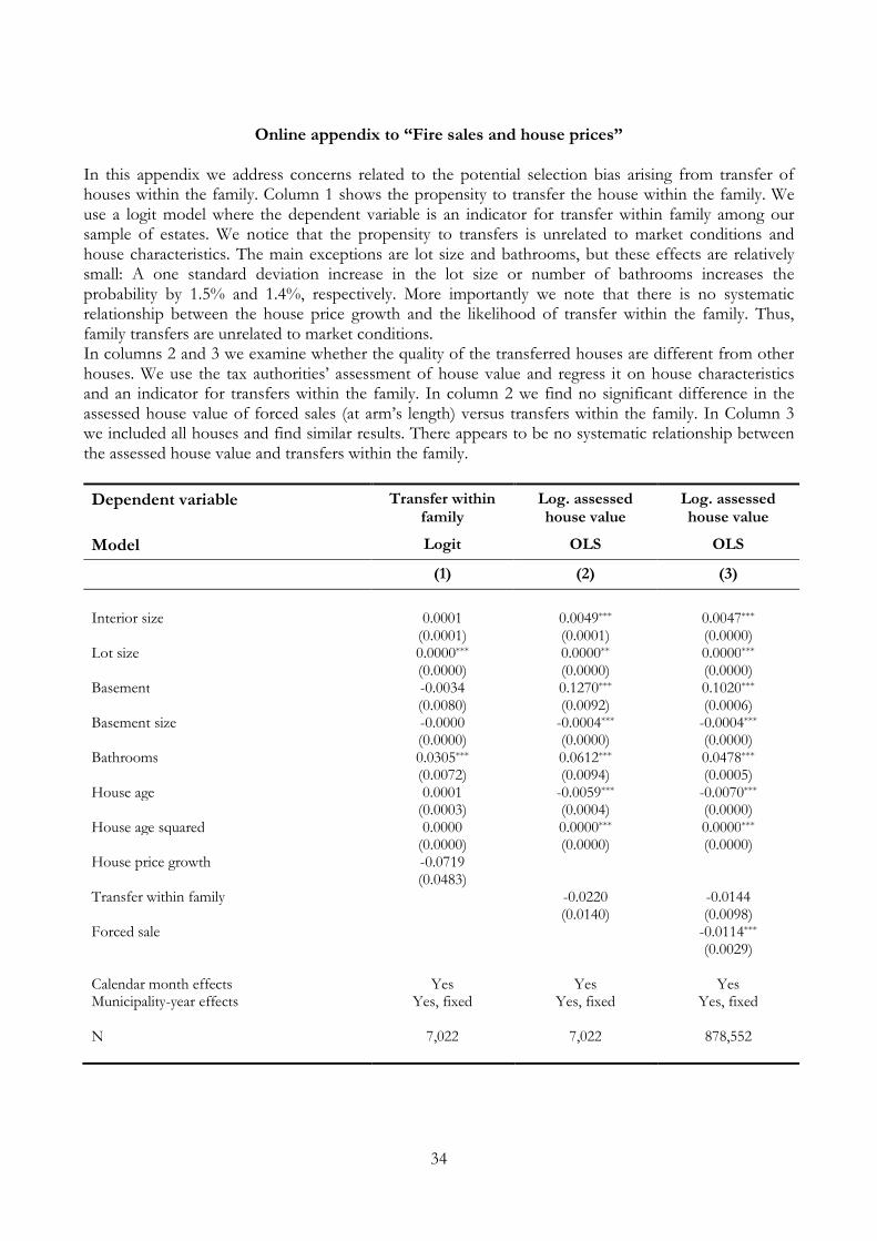
Online appendix to “Fire sales and house prices” In this appendix we address concerns related to the potential selection bias arising from transfer of houses within the family. Column 1 shows the propensity to transfer the house within the family. We use a logit model where the dependent variable is an indicator for transfer within family among our sample of estates. We notice that the propensity to transfers is unrelated to market conditions and house characteristics. The main exceptions are lot size and bathrooms, but these effects are relatively small: A one standard deviation increase in the lot size or number of bathrooms increases the probability by 1.5% and 1.4%, respectively. More importantly we note that there is no systematic relationship between the house price growth and the likelihood of transfer within the family. Thus, family transfers are unrelated to market conditions. In columns 2 and 3 we examine whether the quality of the transferred houses are different from other houses. We use the tax authorities’ assessment of house value and regress it on house characteristics and an indicator for transfers within the family. In column 2 we find no significant difference in the assessed house value of forced sales (at arm’s length) versus transfers within the family. In Column 3 we included all houses and find similar results. There appears to be no systematic relationship between the assessed house value and transfers within the family.

Dependent variable Transfer within family

Log. assessed house value

Log. assessed house value

Model Logit OLS OLS

(1) (2) (3)

Interior size 0.0001

(0.0001) 0.0049*** (0.0001)

0.0047*** (0.0000)

Lot size 0.0000*** (0.0000)

0.0000** (0.0000)

0.0000*** (0.0000)

Basement -0.0034

(0.0080) 0.1270***

(0.0092) 0.1020***

(0.0006) Basement size -0.0000 -0.0004*** -0.0004*** (0.0000) (0.0000) (0.0000) Bathrooms 0.0305***

(0.0072) 0.0612***

(0.0094) 0.0478***

(0.0005) House age 0.0001

(0.0003) -0.0059*** (0.0004)

-0.0070*** (0.0000)

House age squared 0.0000

(0.0000) 0.0000***

(0.0000) 0.0000***

(0.0000) House price growth -0.0719

(0.0483)

Transfer within family -0.0220 (0.0140)

-0.0144 (0.0098)

Forced sale -0.0114*** (0.0029)

Calendar month effects Yes Yes Yes Municipality-year effects Yes, fixed Yes, fixed Yes, fixed N 7,022 7,022 878,552