asset fire sales in equity markets - university of virginia · · 2005-03-28in addition, future...

Asset Fire Sales (and Purchases) in Equity Markets

JOSHUA COVAL AND ERIK STAFFORD*

March 2005

ABSTRACT:

This paper examines asset fire sales, and institutional price pressure more generally, in equity markets, using market prices of mutual fund liquidations caused by capital flows from 1980 to 2003. Forced transactions are a significant cost of financial distress for mutual funds. We find that buyers in asset fire sales earn highly significant returns for providing liquidity when few others are willing or able. In addition, future asset fire sales are predictable, creating an incentive to front-run the anticipated forced sales by distressed funds.

* Coval and Stafford are at Harvard University. We thank Malcolm Baker, David Scharfstein, and Tuomo Vuolteenaho for valuable comments and discussions, and seminar participants at Harvard Business School.

1

This paper assesses the costs of asset fire sales in equity markets. Financial distress is

costly whenever a firm’s past financing decisions interfere with current operations. One

situation where this arises is when capital providers force a firm to quickly sell specialized

assets. Because the sale is immediate, the liquidity premium can be large, resulting in

transaction prices that are substantially below their fundamental values. Equity markets are

relatively liquid, but not perfectly so. Largely because of the high liquidity in equity markets,

many firms that specialize in equity investing are willing to allow capital providers to withdraw

their capital on demand. Evidence presented in this paper suggests that even in the most liquid

of markets, assets sometimes sell at fire sale prices.

Shleifer and Vishny (1992) analyze the equilibrium aspect of asset sales and describe a

situation where liquidity can disappear, making it very costly for someone who is forced to sell.

They essentially argue that asset fire sales are possible when financial distress clusters through

time at the industry level and firms within an industry have specialized assets. When a firm must

sell assets because of financial distress, the potential buyers with the highest valuation for the

specialized asset are other firms in the same industry, who are likely to be in a similarly dire

financial situation, and therefore will be unable to supply liquidity. Instead, liquidity comes

from industry outsiders, who have lower valuations for the asset, and thus bid lower prices.

This story can be recast easily in a capital market setting. Here, the firms are professional

investors, who follow somewhat specialized investment strategies. In this context, specialization

refers to concentrated positions in securities that have limited breadth of ownership, but

importantly, have significant overlap with others following a similar strategy.1 Specialization is

common in investment management, with many professional investors focusing on a single or

limited number of investment strategies. Merton (1987) and Shleifer and Vishny (1997) present

models of investment management that rely on specialization to derive limited arbitrage.

1 For example, merger arbitrage is a specialized investment strategy followed by many professional investors, requiring relatively large positions in stocks that eventually are held mainly by merger arbitrageurs.

2

Financial distress occurs when a firm struggles to make payments required by its liabilities,

which for a financial firm arises when investors redeem their capital. When capital is

immediately demandable, a poorly performing mutual fund without significant cash reserves has

no choice but to sell holdings quickly, which will be costly if too many others are selling the

same positions at the same time. If immediacy is not required, the seller can wait for better

pricing, raise additional funds, or potentially renegotiate existing claims. However, these are not

legitimate options for a poorly performing fund. Renegotiation with large numbers of claim

holders is infeasible, and raising additional funds from new investors, while existing investors

want out, is highly unlikely. Regulations prevent mutual funds from raising funds by short

selling other securities, and binding margin constraints are likely to restrict short selling by

severely underperforming hedge funds.2

Accurate assessment of asset fire sale costs requires considerable transparency in the

decisions of the firm and its investors, whereas most settings in which asset fire sales are costly

are likely to be highly opaque. The primary challenge in measuring the costs of asset fire sales is

that distinguishing financial from economic distress requires identifying asset sales that are a

direct consequence of the financing decisions of the firm. In many corporate settings, financial

difficulties and economic difficulties coincide over multi-year periods, making causality difficult

to assign. Additionally, efficient estimation of costs requires precise measurement of fair asset

value, which can be a challenge in environments characterized by illiquidity and declining

prices.

The focus of this paper is on the assets held by open-ended mutual funds. The open-

ended mutual fund structure produces a highly transparent firm with investment decisions that

2 The asset fire sale story is similar to the price pressure hypothesis of Scholes (1972), where stock prices can diverge from their information-efficient values because of uninformed shocks to excess demand to compensate those who provide liquidity. The asset fire sale story identifies forced selling by distressed mutual funds as one particular type of uninformed shock, and explains why those who provide liquidity during such a crisis are likely to demand additional compensation.

3

are easy to identify and monitor. The opened mutual fund is also extremely reliant on outside

capital to fund its investment opportunities – only the occasional back-end load stands between

outside capital providers and their capital. Monthly reporting of total net assets allows real time

measurement of the pressures that outside capital providers place on the firm. Moreover,

because of high trading frequency in public markets, deviations in transaction prices from fair

values can be accurately assessed via the tracking of post-sale returns. On the other hand, the

stock market environment is a relatively hospitable one for asset sales. With high transaction

volumes and low execution costs, a distressed seller of a listed equity might expect to find many

willing buyers. In addition, mutual funds that select the open-ended organizational form do so

precisely because they view the potential costs of this structure to be low.3 Thus, our focus is on

a setting where asset fire sales are unlikely, but where high transparency permits them to be

properly detected should they exist.4

To examine empirically asset fire sales in equity markets and the effects of institutional

price pressure more generally, we construct a sample of situations where we suspect widespread

mutual fund trading of individual stocks caused by capital flows. Fundamental value is not

immediately observable, but by studying systematic patterns in abnormal returns over time, we

can identify deviations between transaction prices and fundamental value ex post if we find

evidence of significant price reversals following forced transactions. We attempt to disentangle

price pressure from information effects by focusing on situations where the fire sale story

predicts that mutual fund sales are motivated by necessity, as opposed to opportunistic

information-based trading. In particular, we focus on mutual funds stock transactions that are

forced by financial distress, and therefore unlikely to reveal much new information about the

individual securities being sold, and where there is considerable overlap in the holdings among

3 Stein (2004) presents a model where competition pushes mutual funds toward the open-end form even though this severely constrains their ability to conduct arbitrage trades. 4 See Andrade and Kaplan (1998), Asquith, Gertner, and Scharfstein (1994), Gilson (1997) for studies of financially distressed firms. See Pulvino (1998) for a study focusing on asset fire sales.

4

poorly performing funds. The empirical results provide considerable support for the view that

concentrated mutual fund sales forced by capital flows exert significant price pressure in equity

markets, often resulting in transaction prices far from fundamental value.

We find that poor performance leads to capital outflows for mutual funds, the most

serious of which, we consider financial distress. This corroborates previous research, which

finds a strong relation between mutual fund flows and past performance.5 Interestingly, funds

who find themselves in the bottom decile of capital flows tend to be less diversified than other

funds, holding nearly 25% fewer securities than a typical fund.

The analysis also indicates that flows into and out of mutual funds do indeed force

trading. Mutual funds in the bottom decile of capital flows are roughly twice as likely to sell, or

eliminate holdings, than funds experiencing normal flows. This forced trading is especially

costly for mutual funds when there is significant overlap with the securities held by other funds

experiencing outflows, where transactions appear to occur far from fundamental value. We

estimate that investors providing liquidity to the distressed funds earn significant abnormal

returns over the subsequent months. Moreover, we show that forced transactions are predictable,

which creates an opportunity for front-running. An investment strategy, which short sells stocks

most likely to be involved in fire sales, and buys ahead of anticipated forced purchases, earns

average annual abnormal returns well over 15%.

Finally, we document that concentrated mutual fund buying and selling caused by capital

flows is highly related to the momentum effect found in equity returns, but that a considerable

abnormal return remains after controlling for momentum. Because mutual fund flows are

sensitive to past performance, the stocks that mutual funds are forced to sell tend to overlap with

the stocks identified as good shorts by a momentum strategy.

This paper is organized as follows. Section I describes the data. Section II presents

evidence on the existence and magnitudes of price pressure and asset fire sales in equity markets.

5 See for example, Ippolito (1992), Chevalier and Ellison (1997), and Sirri and Tufano (1998)

5

Section III examines the incentives for providing liquidity during crisis periods and for front-

running. Section IV discusses the persistence of institutional price pressure, and Section V

concludes.

I. Data Description

A. Mutual Fund Holdings, Returns, & Flows

Most of our analysis relies on a merger of the two major mutual fund databases that have

been used extensively in the literature: the Spectrum mutual fund holdings database and the

CRSP mutual fund monthly net returns database. Comprehensive descriptions of both can be

found in Wermers (1999), who conducts a similar merge.

Our merge procedure is as follows. First, funds are matched by name. To make sure we

have identified the timing of changes in holdings accurately, we only include fund-quarter

observations reported across adjacent quarters when holdings changes are required. Fund-

quarter observations where the value of the holdings differs substantially from that reported in

the CRSP database net of the cash position are removed. Because our focus is on US equity

funds, we exclude funds with an investment objective code indicating any of the following:

international; municipal bonds; bonds and preferred; or metals. Finally, because the number of

matched funds is significantly lower in the 1980s than in the 1990s, we often emphasize the

subperiod from 1990 through 2003, in our analysis.

Mutual fund flows are estimated using the CRSP series of monthly total net assets (TNAs)

and returns. The net flow of funds to mutual fund j, during month t is defined as:

)1( ,1,,, tjtjtjtj RTNATNAFLOW +⋅−= − (1)

1,

,,

−

=tj

tjtj TNA

FLOWflow (2)

where TNAj,t is the CRSP TNA value for fund j at the end of month t, and Rj,t is the monthly

return for fund j over month t. In order to match with the quarterly holdings data, we sum

6

monthly flows over the quarter to calculate quarterly flows. Most of the analysis involving

mutual fund flows uses FLOW as a percentage of beginning of period TNA as in equation (2).

B. Measuring the Relation between Fund Performance and Flows

It is well documented that capital flows to and from mutual funds are strongly related to

past performance (e.g. Sirri and Tufano (1998)). We use a simple Fama-MacBeth (1973) style

regression model to forecast fund flows based on past returns and lagged flows.

∑∑=

−=

− ⋅+⋅+=8

1,

4

1,,

hhtjh

kktjktj Rcflowbaflow (3)

In particular, each quarter or month, t, we estimate a cross-sectional regression as in (3). We

then calculate the time series average of the coefficients and report t-statistics using the time

series standard error of the mean. Expected flows are calculated as the fitted values using the

time series average of the coefficients.

We estimate the regressions coefficients using a sub-sample of the quarterly mutual fund

observations that we view as having the most reliable data. In particular, we impose the

following data requirements:

• MTNA tj 1$ had,point someat havemust Fund , >

• At some point, fund must have had at least 20 holdings

• Changes in TNA cannot be too extreme, in particular: 0.250.01,

, <∆

<−−tj

tj

TNATNA

• Data from CRSP and Spectrum cannot be too different: 3.13.1

1

,

, << Spectrum

CRSP

tj

tj

TNATNA

7

The coefficients from the sub-sample regressions are used to calculate expected flows for all

funds, including those excluded from the estimation. Results are not meaningfully altered, if the

funds excluded from the regressions are completely dropped from the analysis altogether.

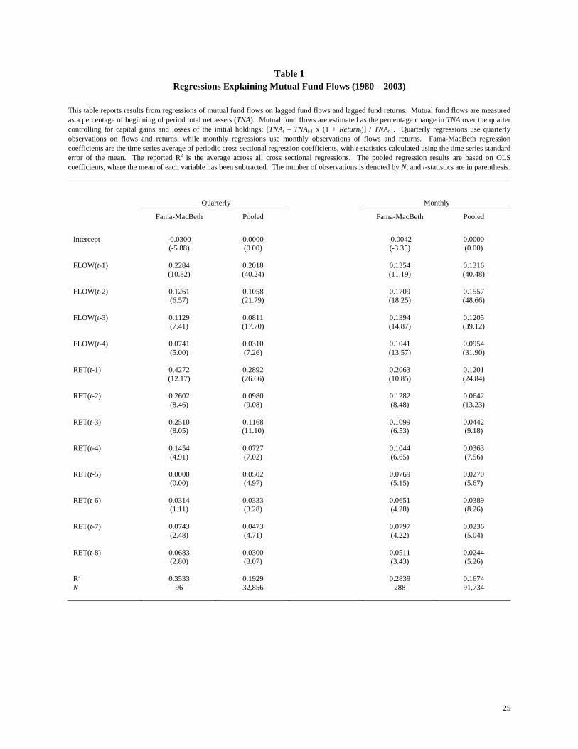
Table 1 reports regression results. As expected from previous research, there is a strong

relation between mutual fund flows and both lagged flows and lagged returns. Quarterly mutual

fund flows are highly significant in explaining future flows for up to a full year, while quarterly

fund returns are important determinants of future flows for two years. The results are highly

consistent with pooled regression results. The main distinction is that the explanatory variables

in the Fama-MacBeth regression focus on explaining cross-sectional differences in flows

whereas the pooled regression coefficients must also account for time-series variation in overall

flows. As a result, the Fama-MacBeth coefficients are estimated more precisely, relative to the

number of observations.

C. Fund Behavior in Response to Financial Pressure

Our notion of a stock fire sale requires that several different owners, who are each

experiencing financial distress, contemporaneously sell the security. Mutual funds experiencing

significant outflows have no choice but to sell some of their holdings to cover redemptions

unless they have excess cash or can borrow. Typically, borrowing is difficult and, because most

funds are evaluated against all-equity benchmarks, few maintain significant cash balances.

Moreover, short selling other securities is usually not feasible. Therefore, the immediate selling

of some existing holdings is the only option. In addition, it is important that there are many

sellers relative to potential buyers. A single fund selling when others are willing and able to

provide liquidity is unlikely to produce a fire sale price. Only when many funds are forced to

sell the same security should we expect to see significant price pressure.

Table 2 provides an overview of fund behavior in response to financial pressure. In

Panels A and B, we sort funds into deciles according to actual and expected quarterly flows. We

then calculate the fraction of a given fund’s positions that are maintained, expanded, reduced, or

8

eliminated during the given quarter and average these values across funds within each decile.

We also report for each decile the average 12-month fund return and the average number of

holdings. In Panels C and D, we average at the holding level, reporting the fraction of holdings

within each decile that are maintained, expanded, reduced, or eliminated.

As Table 2 makes clear, fund flows have a strong impact on fund trading behavior. In

particular, funds experiencing (or expected to experience) large outflows are far less likely to

expand or maintain existing positions and far more likely to reduce or eliminate positions. For

instance, a holding that ranks in the top decile of fund outflows has a 54.8% chance of being

reduced or eliminated by its fund, whereas a holding in the bottom decile has a 20% chance of

being reduced or eliminated. A similar pattern exists for holdings of funds that are expected to

experience outflows during the current quarter. Holdings of funds in the top decile of expected

outflows are 48.4% likely to be reduced or sold versus 27.4% for holdings by funds in the

bottom decile. Finally, funds experiencing outflows tend to be less well diversified than those

experiencing inflows. Funds in the top decile of outflows average 82.8 holdings, whereas funds

in the bottom decile average 102.9. Although the number of holdings is an imprecise measure of

diversification, it is consistent with the idea that specialized funds may be more sensitive to the

costs of financial distress.

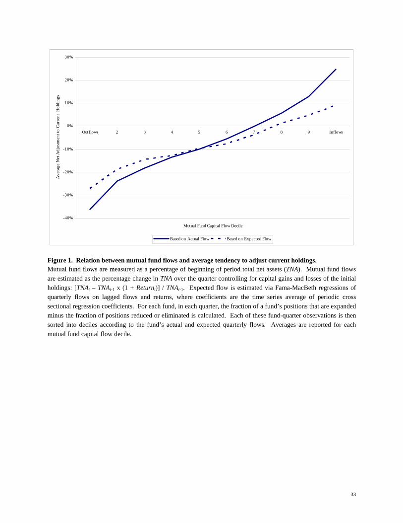
Figure 1 displays the average tendency of net adjustments to existing positions as

function of capital flows. This is merely a graphical representation of some of the data from

Table 2. Consistent with the fire sale story, the funds with the most significant outflows are very

likely to reduce their existing positions. However, the figure clearly shows that there is a similar

effect caused by inflows. Funds in the top decile of capital flows tend to increase their existing

positions. This is interesting, because unlike the firms who must sell in the face of outflows,

these funds have more options. These funds can accumulate cash or purchase securities that they

do not currently own, neither of which is feasible for firms facing outflows.

9

As argued above, these fund-level responses to outflows are unlikely to result in any

significant price pressure unless a stock finds itself with many forced sellers and few willing

buyers.

D. Identifying Fire Sales

A natural measure of asset fire sales might be to determine the number of shares sold due

to capital outflows and scale by the number of shares outstanding or trading volume. There are

two reasons why such a measure is likely to be highly misleading. First, as argued above, fund-

level responses to outflows are unlikely to result in any significant price pressure unless a stock

finds itself with many forced sellers and few willing buyers. A large investor can orderly

liquidate a large position, but a large number of small investors cannot orderly liquidate a similar

size aggregate position. This makes it important for a measure to emphasize commonality in the

capital flows to investors of a particular security. A second weakness of share-based measures of

asset fire sales is that they are highly sensitive to reporting errors in fund holdings. Because

funds are only required to report their holdings on a semi-annual basis, Spectrum relies on

voluntary disclosure to fill in off-quarter holdings. This results in a non-trivial frequency of

errors in reported holdings and places a significant burden on share-based measures to identify

them as such.

In view of the above considerations, our procedure for classifying mutual fund stock sales

as asset fire sales (and purchases) is as follows. First, we identify transactions by funds that are

likely forced by capital flows. In particular, we define quarterly forced sales (buys) as decreases

(increases) in holdings by funds experiencing concurrent outflows (inflows) greater than 5%.

The difference between forced buys and forced sales is then scaled by the total number of mutual

fund owners, to form a variable we call PRESSURE.6

6 We require at least 10 mutual funds owners before we calculate the PRESSURE variable.

10

( ) ( )

∑∑∑

−

−<−>=

j tij

j tjtijj tjtijti Own

flowSellflowBuyPRESSURE

1,,

,,,,,,,

%5|%5| (4)

Buyj,i,t equals one if fund j increased its holding in stock i during quarter t, and zero otherwise.

Sellj,i,t is defined similarly based on decreases. Stocks with PRESSURE ≤ -15% are determined

to be fire sale stocks, and those with PRESSURE ≥ 25% are determined to be fire purchase

stocks.

II. Price Effects of Mutual Fund Sales & Fire Sales

In general, detecting price pressure effects around mutual fund stock transactions is

problematic because of the simultaneous effects of price pressure and information revelation. In

an attempt to disentangle price pressure and information effects, we examine stock price changes

around widespread forced and unforced mutual fund sales, and look for evidence of stock price

drops followed by a significant price reversal.7 If mutual funds bring information into prices

through their trading, then we should see a price drop in the period where they are selling

heavily, and then no drift in abnormal returns following the trades. However, if mutual fund

trading is driven by necessity rather than information, and if this forced trading results in fire sale

prices, then we should see a significant price drop over the period where they are being forced to

sell, followed by a period of positive abnormal returns compensating those who provided

liquidity in the crisis period.

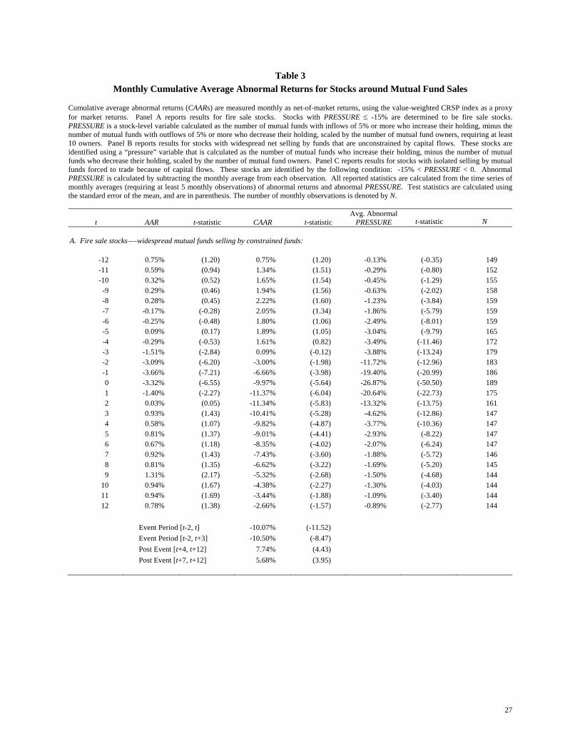
Table 3 displays monthly abnormal returns around various types of mutual fund stock

transactions. Monthly abnormal returns are calculated using simple net-of-market returns, where

the CRSP value-weighted index proxies for the market portfolio. In the spirit of Fama and

MacBeth (1973), we calculate average abnormal returns each month and then use the time series

of mean abnormal returns for statistical inference to control for potential cross-sectional

7 This empirical approach is similar to the one used by Mitchell, Pulvino, and Stafford (2004) who study price pressure around mergers.

11

dependence in the monthly abnormal returns.8 The fire sale sample is selected according to the

procedure described in the previous section, where stocks with widespread selling by distressed

funds are considered fire sale stocks. Table 3 also reports the average abnormal value of our

pressure variable for easy comparison to the associated monthly abnormal returns.

In Panel A, the pattern in average abnormal returns around the widespread selling of

stocks held by distressed mutual funds is striking. We find significantly negative abnormal

returns in the months of forced selling and those immediately surrounding them. Over the

quarter where, on net, at least 15% of the owners are distressed sellers of the same stock9, the

average abnormal stock return is -10.1% with a t-statistic of -11.52. There is some spillover in

stock price performance into the next month, with average abnormal returns of -1.4%, as net

forced selling remains high. Over the quarter where fire sales are occurring, roughly 20% of the

owners are on average net forced sellers of each stock, and this amount of forced selling pressure

continues into the subsequent month.

Importantly, the downward pattern in abnormal returns eventually reverses once the net

forced sales dissipate. From months 4 to 12 following the fire sale quarter, average abnormal net

forced selling pressure retreats to under 2%, and stock prices for the fire sale stocks rebound

7.74%% over this period, with a t-statistic of 4.43. The rebound does not fully cover the losses

associated with the initial price drop, but represents a significant cost of a fire sale. This

evidence suggests that widespread forced selling by distressed mutual funds exerts significant

downward price pressure on the individual stocks sold, well beyond any contemporaneous

information effects.

In Panels B and C, we explore the role of each ingredient of the fire sale⎯widespread net

selling pressure, by constrained funds. When there is widespread selling by unconstrained funds,

8 This procedure gives equal weight to each monthly observation, rather than each individual observation. When individual observations are given equal weight and assumed independent, the patterns are more pronounced with highly significant test statistics. 9 Months -2, -1, and 0 define the event quarter.

12

the striking fire sale pattern in abnormal returns is not present. Panel B of Table 3 reports

CAARs around similarly widespread mutual fund sales, but by funds that are not necessarily

forced to sell. In particular, this sample is again identified using a “pressure” variable, but one

altered by removing the condition on flow from the calculation. Again, there is a significant

price drop over the quarter of widespread selling, with some continuation into the next quarter.

However, the reversal is much more modest. In fact, the fire sale stocks that are part of this

unconditional sample are driving most of the reversal. This is consistent with voluntary mutual

fund trading bringing information into prices, and on average, prices adjusting to an appropriate

level.

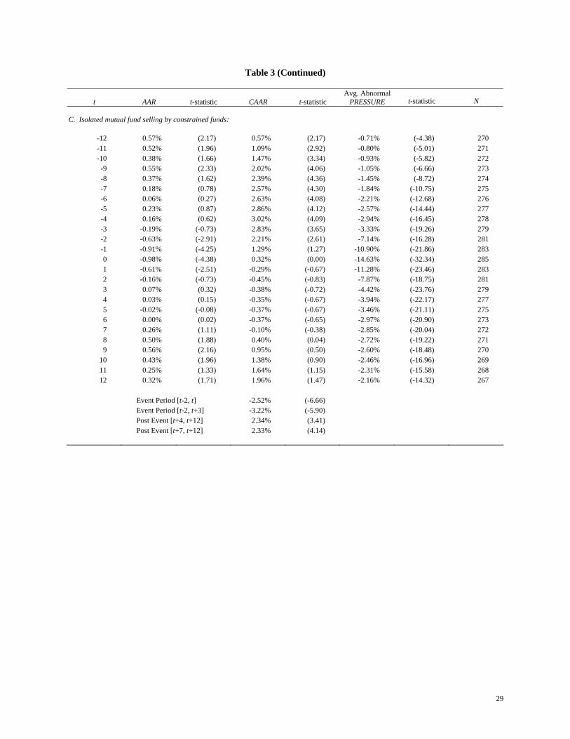
In Panel C of Table 3, we report results for a sample of mutual fund sales by distressed

funds, where the selling is isolated. We identify the sample based on the following condition:

-15% < PRESSURE < 0. In the case of isolated distressed selling, there is a modest, but

statistically significant, average abnormal stock price drop of -2.52% (t-statistic = -6.66) over the

event quarter, with most of this drop being reversed over the subsequent quarters. Although the

pattern in CAARs is statistically significant, the economic magnitudes are fairly small.

The key to the reversal appears to be that the selling is widespread among mutual funds

that must immediately sell due to capital outflows. Moreover, the effect seems to be increasing

in the number of net sellers and in the level of distress. Figure 2 illustrates the “comparative

statics” with nine graphs representing various proportions of net sellers with varying degrees of

distress. In particular, the top row displays unconstrained funds, the middle row shows funds

with |flows| > 5%, and the bottom row reports funds with |flows| > 10%. The proportion of net

sellers varies across the columns, with at least 5% of owners selling in the first column, at least

15% of owners selling in the second column, and at least 25% of owners selling in the third

column. The center graph corresponds to the fire sale sample (results in Panel A of Table 3).

The fire sale pattern becomes more extreme moving down and/or to the right, suggesting that the

intensity of fire sales is increasing in both of these factors. For example, when we hold the

capital flows threshold constant at |flows| >5% and increase the proportion of net sellers

13

threshold from “at least 15%” to “at least 25%” the average abnormal return from month t-2 to

t+3 is -18.13% (t-statistic = -7.58) with a reversal of 15.01% (t-statistic = 3.84) over the next 3

quarters. Likewise, holding the proportion of net sellers threshold at “at least 15%” and

increasing the flows threshold to |flows| >10% results in an average abnormal return from month

t-2 to t+3 of -13.02% (t-statistic = -6.36) with a full reversal of 14.57% (t-statistic = 4.93) over

the next 3 quarters.

The results also reveal something about which stocks are sold in response to significant

outflows. The abnormal returns for the fire sale stocks prior to the actual sale are close to zero

(slightly positive, but only marginally statistically insignificant). This suggests that these stocks

have performed relatively well when compared to the market, and extremely well relative to the

distressed funds’ average holdings. For the most part, the distressed funds have been

significantly underperforming the market. In particular, the cumulative average abnormal return

over the nine months prior to the fire sale quarter for the distressed funds is -4.5% (t-statistic =

-7.40). Thus, it appears that in crisis periods, struggling funds sell relative “winners” rather than

downside momentum stocks. We are presumably observing outcomes from optimized behavior,

suggesting that the sale of “loser” stocks during these crisis periods would result in more severe

price discounts.

Finally, the persistence in net forced selling is interesting. Not all funds experience

outflows at the exact same time. The initial widespread forced sales can create an externality for

the marginal funds that would not face capital withdrawals in the absence of this price pressure.

However, their performance is sufficiently affected by the fire sales themselves, that they face

outflows the subsequent quarter, which forces them to sell with a lag. This is related to an effect

described in Mitchell, Pulvino, and Stafford (2002) created by margin requirements. A firm up

against a financing constraint (i.e. facing a margin call) may have to sell, and in so doing,

adversely impact prices for others following a similar strategy. Here, the financing constraint is

not only binding, but also actually tightening, as capital providers withdraw funds. Interestingly,

this sequence of events creates persistent mispricing, which can get worse before being

14

eliminated, and does not presuppose irrational investors or managers. This externality can be an

important impediment to arbitrage in imperfect capital markets (Shleifer and Vishny (1997)).

III. Incentives for Providing Liquidity & Front-Running

The event-time analysis presented in the previous section suggests that there may be a

strong incentive to provide liquidity at times of widespread selling by financially distressed

mutual funds. In other words, the buyers in asset fire sales are receiving attractive prices for

providing liquidity when few others are able or willing. In addition, because capital flows are

predictable, there may also be an incentive to remove liquidity in anticipation of forced sales by

front-running the distressed mutual funds. We investigate both of these incentives by studying

the portfolio returns to investors following these investment strategies.

A. Investment Returns following Asset Fire Sales

The results displayed in Table 3 suggest that the buyer in an asset fire sale will, on

average, be compensated for providing liquidity. The compensation is realized as prices return

to their information-efficient values in the subsequent months, and can be detected in the form of

positive abnormal returns. To measure investment performance to buyers in asset fire sales, we

calculate the calendar-time portfolio returns to an investment strategy that buys all stocks

identified as fire sale stocks within the past year, but not within the most recent quarter. The

constraint that the fire sale has not occurred within the most recent quarter ensures that this is a

feasible investment strategy in terms of all required information being publicly available. A

secondary benefit of this constraint is that it avoids the spillover of fire sales into the subsequent

month. Measuring abnormal returns requires a model of expected returns. We report results

using three different models: CAPM, Fama-French 3-factor model, and a 4-factor model that

15

includes momentum (see Fama and French (1993) for a description of the construction of the

factors).10

tttttttt eUMDuHMLhSMBsRfRmbaRfRp +⋅+⋅+⋅+−⋅+=− ][

(5)

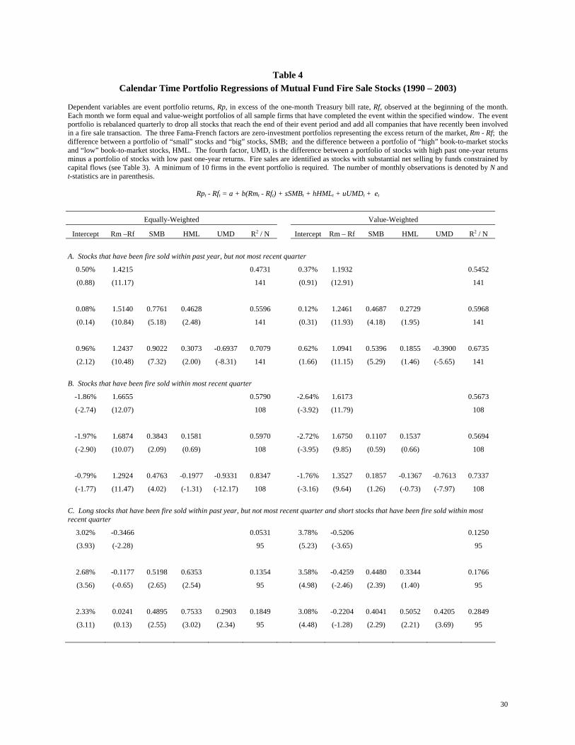
Table 4 reports calendar-time portfolio regressions of the investment strategy described

above for both equal-weight and value-weight portfolios. The intercept from these regressions

represents the average monthly abnormal return, given the model. The intercepts reported in

Panel A, range from a mere 8 basis points (bps) per month (t-statistic = 0.14), to just under 1.0%

per month (t-statistic = 2.12), and are remarkably similar between equal- and value-weighted

portfolios. However, only the equal-weight portfolio has a statistically significant intercept, and

this only after controlling for momentum. This is an extremely volatile stand-alone investment

strategy. The negative loading on momentum is interesting, suggesting that these stocks covary

significantly with downside momentum stocks, but have not performed poorly themselves.

Another interesting feature of these portfolios is the large estimated coefficient on the market

excess return.

The second panel in Table 4 displays performance results for an investment strategy that

“piles on” to the distressed selling that occurred in the prior month. This strategy, rather than

providing liquidity, is competing for liquidity, and therefore exacerbating the price pressure.

This is arguably a less feasible strategy requiring immediate access to the mutual fund holdings

data at the end of each quarter, but still conditional only on previous transactions. The economic

magnitude of the abnormal returns is very large, and usually associated with strong statistical

reliability. Five of the six investment strategies result in statistically significant abnormal returns

at traditional significant levels, ranging from -0.79% per month (t-statistic = -1.77), to -2.72%

per month (t-statistic = -3.95). Controlling for momentum reduces the intercepts by roughly half.

In many regards, this investment strategy is very similar to a momentum strategy. In both cases,

10 The factors are from Ken French: http://mba.tuck.dartmouth.edu/pages/faculty/ken.french/data_library.html.

16

the portfolio contains stocks that have performed poorly, and continue to underperform.

However, the mechanism that creates the low returns appears to be the continued forced selling

by distressed mutual funds in one case, while unspecified in the case of momentum. Again, the

beta estimates are very large. In the CAPM regressions, the estimated beta is 1.7 for both the

equal- and value-weighted portfolios.

The final panel in Table 4 shows the results from combining the two strategies described

above into a long-short investment strategy. The same basic pattern emerges. The returns are

somewhat more extreme with the value-weighted portfolios; extremely large in economic terms,

with annualized abnormal returns ranging from 27.9% (t-statistic = 3.11) to 45.4% (t-statistic =

5.23), and fairly strong statistical reliability. Note that because of combining two strategies into

a long-short strategy, and requiring at least 10 firms in each of the long and short portfolios, that

the number of months that this strategy is feasible drops to only 95 months out of a possible 168

months. Therefore, the abnormal return estimates overstate the true investment returns by

ignoring the capital costs of standing idle.11

B. Investment Returns following Asset Fire Purchases

The evidence in Table 2 and Figure 1 suggest that funds with significant capital inflows

tend to increase their existing holdings; much like the funds experiencing significant outflows

tend to reduce their existing positions. In other words, funds facing significant inflows behave as

if they too are constrained. As in the fire sale story, if many funds are simultaneously forced to

buy the same securities when few others are able to sell, transaction prices may occur at a price

significantly above fundamental value, what we will call asset fire purchases.

We identify asset fire purchases using the PRESSURE variable. In particular, when

PRESSURE > 25% we consider the stock to be involved in as asset fire purchase. To measure

11 Myron Scholes describes liquidity-related strategies like this as “fire-station” strategies, where much of the time is spent standing around waiting for an event, while costs are incurred continuously.

17

investment performance to sellers in asset fire purchases, we calculate the calendar-time

portfolio returns to an investment strategy that buys all stocks identified as fire purchase stocks

within the past year, but not within the most recent quarter. Again, we also examine the strategy

of “piling on” to the asset fire purchase, and a long-short strategy that combines the two

strategies. If asset fire purchases result in significant price pressure, then we should see positive

abnormal returns to the piling on strategy, followed by a reversal.

Table 5 reports calendar-time portfolio regressions of the investment strategy described

above for both equal-weight and value-weight portfolios. The intercepts reported in Panel A

represent the reversal. The average abnormal returns are economically large and all are

statistically significant, ranging from -0.47% per month (t-statistic = -2.15) to -0.84% per month

(t-statistic = -3.41). Interestingly, the monthly abnormal returns remain statistically significant

after controlling for momentum.

The second panel in Table 5 displays performance results for an investment strategy that

“piles on” to the forced buying that occurred over the prior month. Like the earlier piling on

strategy, this one competes for liquidity, and therefore intensifies the price pressure. Again, the

economic magnitude of the abnormal returns is very large, with mixed statistical reliability. Four

of the six investment strategies result in statistically significant abnormal returns, ranging from

0.46% per month (t-statistic = 1.55), to 0.97% per month (t-statistic = 2.59). The value-weight

portfolios tend to produce less extreme abnormal performance, and lower levels of statistical

significance.

Panel C of Table 5 reports the results from combining the previous two strategies into a

single long-short strategy. This strategy produces very large average abnormal returns, all of

which are statistically significant at traditional significance levels. The average abnormal returns

range from 1.11% per month (t-statistic = 3.00) to 1.76% per month (t-statistic = 4.82). The

strategy is highly related to momentum, as both the equal- and value-weighted portfolios have

large positive coefficients on the momentum factor, but intercepts from these regressions are

18

well over 1% per month, suggesting that this effect is somewhat distinct from the momentum

effect.

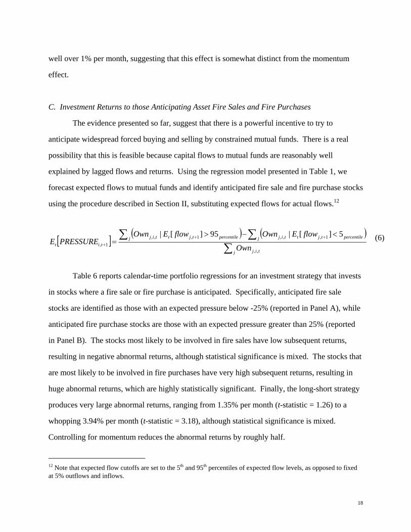
C. Investment Returns to those Anticipating Asset Fire Sales and Fire Purchases

The evidence presented so far, suggest that there is a powerful incentive to try to

anticipate widespread forced buying and selling by constrained mutual funds. There is a real

possibility that this is feasible because capital flows to mutual funds are reasonably well

explained by lagged flows and returns. Using the regression model presented in Table 1, we

forecast expected flows to mutual funds and identify anticipated fire sale and fire purchase stocks

using the procedure described in Section II, substituting expected flows for actual flows.12

[ ] ( ) ( )∑

∑∑ <−>=

++

+

j tij

j percentiletjttijj percentiletjttijtit Own

flowEOwnflowEOwnPRESSUREE

,,

1,,,1,,,1,

5][|95][|

(6)

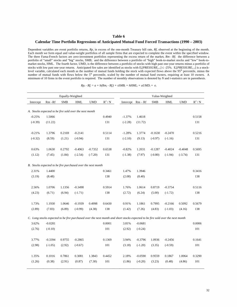
Table 6 reports calendar-time portfolio regressions for an investment strategy that invests

in stocks where a fire sale or fire purchase is anticipated. Specifically, anticipated fire sale

stocks are identified as those with an expected pressure below -25% (reported in Panel A), while

anticipated fire purchase stocks are those with an expected pressure greater than 25% (reported

in Panel B). The stocks most likely to be involved in fire sales have low subsequent returns,

resulting in negative abnormal returns, although statistical significance is mixed. The stocks that

are most likely to be involved in fire purchases have very high subsequent returns, resulting in

huge abnormal returns, which are highly statistically significant. Finally, the long-short strategy

produces very large abnormal returns, ranging from 1.35% per month (t-statistic = 1.26) to a

whopping 3.94% per month (t-statistic = 3.18), although statistical significance is mixed.

Controlling for momentum reduces the abnormal returns by roughly half.

12 Note that expected flow cutoffs are set to the 5th and 95th percentiles of expected flow levels, as opposed to fixed at 5% outflows and inflows.

19

IV. Persistence of Institutional Price Pressure

A. The Role of Information & Agency Costs

Care must be taken in interpreting the calendar-time portfolio regression analysis. The

estimates of average abnormal returns ignore two important costs (Merton (1987)). First, the

estimates of abnormal performance exclude the costs of generally becoming informed about the

investment strategy. Our estimates are based on the period from 1980 to 2003, coinciding with

the availability of the necessary data. Importantly, prices were set over this period by investors

who did not have access to these data, and therefore, their assessments of the risks and returns

associated with the strategy were surely less precise than those presented in the tables. Even

now, the results, while economically enticing, are only marginally significant when taken as a

whole. Second, once the general strategy is recognized as potentially profitable, there are the

information acquisition costs associated with the individual securities, which have not yet been

borne by the eventual liquidity providers. These costs too, are not included in the measured

abnormal returns.

In some sense, we have documented that equities are in fact specialized assets. The fire

sale story begins with the idea that assets are specialized, which, in the short run, fixes the pool

of potential buyers and sellers who fully value the asset. In the case of stocks, where the

information relevant for pricing is costly to obtain, specialization will arise around who has (and

collects) this information. In extreme situations, when a majority of the funds who are informed

about an individual stock are unable to voluntarily trade, price setting may fall on funds who

have not yet invested in the relevant information. These costs are surely positive, and potentially

quite large. The evidence on funds experiencing significant inflows behaving as if they are

constrained is consistent with these costs being large. The fact that these additional costs

occasionally apply produces time variation in transaction costs. Market prices may not be

perfectly efficient, in that prices do not reflect all available information at every point in time,

20

but they may well be within the bounds of time-varying transaction and information costs (a

dynamic version of Grossman and Stiglitz (1980)).

An interesting consequence of significant institutional price pressure in conjunction with

a strong fund performance-flow relation is that the price pressure can spillover into subsequent

periods (Shleifer and Vishny (1997), Shleifer (2000)). There are actually two spillover effects.

One is the own-fund spillover, where a fund’s buying or selling its existing positions

mechanically improves or degrades its own performance, which affects capital flows in the

subsequent period. Another spillover occurs across funds when the initial institutional price

pressure affects marginal funds that would not face capital flows in the absence of this price

pressure. However, their performance is sufficiently affected by the institutional price pressure,

that their capital flows are altered the subsequent quarter, forcing them to transact with a lag.

This sequence of events results in persistent mispricing, which can get worse before being

eliminated.

B. Implications

An interesting implication of the persistent institutional price pressure relates to

performance evaluation of fund managers. Over moderately long periods of several quarters, the

evidence suggests that some portion of performance can, at times, be attributed to price pressure,

which will eventually reverse. In many applications of performance evaluation, one would want

to control for this effect. Additionally, to the extent that fund managers understand these effects,

perverse incentives may exist to exploit the own-fund price pressure of trades to “dress,” or

temporarily enhance, performance, thereby inducing subsequent flows. Since capital flows

appear to be more sensitive to good performance than to poor performance,13 the eventual

reversal of the price pressure will not adversely affect capital flows enough to fully offset the

initial benefits. The likelihood of a single fund being able to create sufficiently persistent price

13 See for example, Chevalier and Ellison (1997), and Sirri and Tufano (1998).

21

pressure as to induce meaningful capital inflows is low, but a fund family may well be able to

coordinate across its own funds to make such a strategy worthwhile.

C. Possibilities for Future Research

The cycle where capital flows can force widespread trading in individual securities,

resulting in institutional price pressure, which in turn affects fund performance and eventually

feeds back into capital flows, is intriguing. Two possible extensions may warrant additional

research. First, the relation to the momentum effect is enticing. This cycle may well describe

the mechanics of why stocks that do well or poorly continue to do so. The evidence presented

here, suggests that the simple liquidity-motivated strategies we examined were highly correlated

with momentum, but offered abnormal returns beyond the momentum factor. A second research

avenue is to examine the role of this cycle in explaining the unusual pricing of technology stocks

in the late 1990s. At the time, casual empiricism suggests that focused sector funds holding

concentrated positions in technology stocks initially outperformed the broader indices, and

consequently received large inflows, which they piled into their existing holdings. This, in turn,

boosted their performance and led to additional inflows.

V. Conclusion

This paper studies asset fire sales, and institutional price pressure more generally, in

equity markets by examining a large sample of stock transactions of mutual funds. We find

considerable support for the notion that widespread selling by financially distressed mutual funds

leads to fire sale prices. Somewhat surprisingly, we find that funds with large inflows behave as

if they too are constrained to quickly transact in their existing positions, on average buying more

of what they already own. When forced purchases are widespread relative to the potential sellers

of individual securities, these forced purchases also result in persistent institutional price

pressure. These findings suggest that even in the most liquid markets there can be a significant

22

premium for immediacy. The price effects are relatively long-lived, lasting around two quarters

and taking several more quarters to reverse. This evidence adds to previous findings of price

pressure effects around index additions and stock-financed mergers. Short-run excess demand

curves for stocks appear to be less than perfectly elastic.

Asset fire sales and purchases are probably the most significant cost of financial distress

for money management firms. Most of these firms have selected an organizational form that

allows capital providers to add or withdraw capital on demand, indicating that the expected costs

of demanding liquidity are low. However, when many funds are forced to transact the same

stocks at the same time, the price impact can be substantial.

The existence of institutional price pressure in equity markets is informative about the

organization of money management firms and, in turn, the effect that these organizations have on

prices. First, it suggests that the costs associated with being informed about an individual

security can be substantial. Merton (1987) argues that large fixed costs of becoming informed

about an investment opportunity can initially limit arbitrage investing, and once they are borne, it

can take a while to learn how best to exploit the opportunity. Moreover, these costs can lead

firms to specialize. Specialization limits their ability to diversify, exposing them to additional

risks, which Shleifer and Vishny (1997) describe as limits to arbitrage. It certainly appears that

many funds follow highly similar strategies, such that there are times when many face

redemptions, and are contemporaneously forced to transact the same securities. In addition, it

seems that it takes a while for forced transactions to be understood by strategy outsiders, creating

time variation in transaction costs, and allowing prices to remain apart from their fundamental

value for several months. Interestingly, the asset fire sale story provides a mechanism for

rational mispricing. The market is clearly somewhat inefficient, in that market prices are not

perfectly reflective of all available information. However, the basis of this mispricing requires

neither irrational investors nor managers. Prices eventually reflect available information, but

sometimes with a significant delay.

23

REFERENCES

Andrade, Gregor, and Steven Kaplan, 1998, How costly is financial (not economic) distress?

Evidence from highly leveraged transactions that became distressed, Journal of Finance

53, 1443-1493.

Asquith, Paul, Robert Gertner, and David Scharfstein, 1994, Anatomy of financial distress: An

examination of junk-bond issuers, Quarterly Journal of Economics 109, 625-658.

Chevalier, Judith and Glenn Ellison, 1997, Risk taking by mutual funds as a response to

incentives, Journal of Political Economy 105, 1167-1200.

Fama, Eugene and James MacBeth, 1973, Risk, Return, and Equilibrium: Empirical Tests,

Journal of Political Economy, 81, 607-636.

Fama, Eugene and Kenneth French, 1993, Common risk factors in the returns on stocks and

bonds, Journal of Financial Economics 33, 3-56.

Gilson, Stuart, 1997, Transaction costs and capital structure choice: Evidence from financially

distressed firms, Journal of Finance 52, 161-197.

Grossman, Sanford J., and Joseph E. Stiglitz, 1980, On the impossibility of informationally

efficient markets, American Economic Review, 393-408.

Ippolito, Richard A., 1992, Consumer reaction to measures of poor quality: Evidence from the

mutual fund industry, Journal of Law and Economics 35, 45-70.

Merton, Robert C., 1987, A simple model of capital market equilibrium with incomplete

information, Journal of Finance 42, 483-510.

24

Mitchell, Mark L., Todd C. Pulvino, and Erik Stafford, 2002, Limited arbitrage in equity

markets, Journal of Finance 57, 551-584.

Mitchell, Mark L., Todd C. Pulvino, and Erik Stafford, 2004, Price pressure around mergers,

Journal of Finance 59, 31-63.

Pulvino, Todd, C., 1998, Do asset fire sales exist? An empirical investigation of commercial

aircraft transactions, Journal of Finance 53, 939-978.

Scholes, Myron, 1972, The market for corporate securities: Substitution versus price pressure

and the effects of information on stock prices, Journal of Business 45, 179-211.

Shleifer, Andrei and Robert Vishny, 1992, Liquidation values and debt capacity: A market

equilibrium approach, Journal of Finance 47, 1343-1366.

Shleifer, Andrei and Robert Vishny, 1997, The limits to arbitrage, Journal of Finance 52, 35-55.

Shleifer, Andrei, 2000, Inefficient Markets: An Introduction to Behavioral Finance (Oxford

University Press).

Sirri, Erik and Peter Tufano, 1998, Costly search and mutual fund flows, Journal of Finance 53,

1589-1622.

Stein, Jeremy, 2004, Why are most mutual funds open-end? Competition and the limits of

arbitrage, Harvard University working paper.

Wermers, Russ, 1999, Mutual fund herding and the impact on stock prices, Journal of Finance

54, 581-622.

25

Table 1 Regressions Explaining Mutual Fund Flows (1980 – 2003)

This table reports results from regressions of mutual fund flows on lagged fund flows and lagged fund returns. Mutual fund flows are measured as a percentage of beginning of period total net assets (TNA). Mutual fund flows are estimated as the percentage change in TNA over the quarter controlling for capital gains and losses of the initial holdings: [TNAt – TNAt-1 x (1 + Returnt)] / TNAt-1. Quarterly regressions use quarterly observations on flows and returns, while monthly regressions use monthly observations of flows and returns. Fama-MacBeth regression coefficients are the time series average of periodic cross sectional regression coefficients, with t-statistics calculated using the time series standard error of the mean. The reported R2 is the average across all cross sectional regressions. The pooled regression results are based on OLS coefficients, where the mean of each variable has been subtracted. The number of observations is denoted by N, and t-statistics are in parenthesis.

Quarterly Monthly

Fama-MacBeth Pooled Fama-MacBeth Pooled

Intercept -0.0300 0.0000 -0.0042 0.0000 (-5.88) (0.00) (-3.35) (0.00) FLOW(t-1) 0.2284 0.2018 0.1354 0.1316 (10.82) (40.24) (11.19) (40.48) FLOW(t-2) 0.1261 0.1058 0.1709 0.1557 (6.57) (21.79) (18.25) (48.66) FLOW(t-3) 0.1129 0.0811 0.1394 0.1205 (7.41) (17.70) (14.87) (39.12) FLOW(t-4) 0.0741 0.0310 0.1041 0.0954 (5.00) (7.26) (13.57) (31.90) RET(t-1) 0.4272 0.2892 0.2063 0.1201 (12.17) (26.66) (10.85) (24.84) RET(t-2) 0.2602 0.0980 0.1282 0.0642 (8.46) (9.08) (8.48) (13.23) RET(t-3) 0.2510 0.1168 0.1099 0.0442 (8.05) (11.10) (6.53) (9.18) RET(t-4) 0.1454 0.0727 0.1044 0.0363 (4.91) (7.02) (6.65) (7.56) RET(t-5) 0.0000 0.0502 0.0769 0.0270 (0.00) (4.97) (5.15) (5.67) RET(t-6) 0.0314 0.0333 0.0651 0.0389 (1.11) (3.28) (4.28) (8.26) RET(t-7) 0.0743 0.0473 0.0797 0.0236 (2.48) (4.71) (4.22) (5.04) RET(t-8) 0.0683 0.0300 0.0511 0.0244 (2.80) (3.07) (3.43) (5.26) R2 0.3533 0.1929 0.2839 0.1674 N 96 32,856 288 91,734

26

Table 2 Mutual Fund Trading in Response to Flows & Expected Flows (1980 – 2003)

This table reports how quarterly mutual fund holdings change conditional on actual and expected flows. Mutual fund flows are measured as a percentage of beginning of period total net assets (TNA). Mutual fund flows are estimated as the percentage change in TNA over the quarter controlling for capital gains and losses of the initial holdings: [TNAt – TNAt-1 x (1 + Returnt)] / TNAt-1. Expected flow is estimated via Fama-MacBeth regressions of quarterly flows on lagged flows and returns, where coefficients are the time series average of periodic cross sectional regression coefficients. In Panels A and B, for each fund in each quarter the fraction of a fund's positions that are maintained, expanded, reduced, or eliminated is calculated. Each of these fund-quarter observations is then sorted into deciles according to the fund's actual (Panel A) and expected (Panel B) quarterly flows. Averages of each variable are reported for each decile. In Panels C and D, holdings are grouped according to the flow (Panel C) and expected flow (Panel D) decile of their associated fund-quarter observation. Within each group, the percentage of holdings that are maintained, expanded, reduced, and eliminated is then calculated. The number of observations is denoted by N. Panel A: Averaging by fund within actual flow deciles

Decile Flow Maintain Expand Reduce Eliminate Prior Fund

Return Average Number

of Holdings 1 -13.6% 31.6% 16.1% 33.7% 18.6% 2.5% 82.8 2 -5.7% 39.3% 18.5% 25.9% 16.4% 0.7% 84.9 3 -3.6% 43.2% 19.3% 22.8% 14.6% 2.9% 89.7 4 -2.3% 47.4% 19.6% 19.9% 13.2% 5.9% 87.7 5 -1.1% 48.8% 20.6% 18.0% 12.6% 8.3% 90.2 6 0.2% 48.0% 23.3% 16.5% 12.2% 9.5% 99.9 7 2.0% 45.1% 27.4% 15.2% 12.3% 12.3% 110.9 8 4.8% 41.3% 32.2% 14.0% 12.5% 13.4% 122.5 9 10.6% 36.4% 38.3% 12.4% 12.9% 16.8% 122.2

10 41.8% 26.2% 49.3% 10.0% 14.5% 21.1% 102.9

Panel B: Averaging by fund within expected flow deciles

Decile E[Flow] Maintain Expand Reduce Eliminate Prior Fund

Return Average Number

of Holdings 1 -14.1% 29.4% 21.8% 30.5% 18.4% -26.4% 92.5 2 -7.7% 39.4% 20.9% 24.5% 15.2% -11.8% 102.2 3 -4.4% 42.9% 21.3% 22.0% 13.8% -3.3% 93.4 4 -2.1% 46.4% 20.4% 20.0% 13.2% 3.4% 89.6 5 -0.2% 47.1% 21.6% 18.9% 12.4% 8.6% 99.0 6 1.5% 47.4% 22.5% 18.2% 12.0% 13.0% 102.1 7 3.3% 46.5% 24.9% 16.8% 11.9% 17.1% 100.0 8 5.5% 44.1% 28.6% 15.5% 11.9% 21.1% 115.3 9 8.9% 39.7% 32.5% 15.1% 12.7% 26.3% 118.8

10 19.8% 30.9% 39.1% 14.9% 15.1% 35.5% 104.5

Panel C: Averaging by holding within actual flow deciles Decile Flow Maintain Expand Reduce Eliminate Prior Return N

1 -14.0% 28.2% 17.0% 39.2% 15.6% 23.9% 432,652 2 -5.7% 37.5% 19.5% 29.0% 14.1% 20.2% 436,773 3 -3.6% 39.9% 19.6% 28.0% 12.6% 19.6% 457,031 4 -2.3% 43.0% 21.6% 24.1% 11.3% 20.4% 445,800 5 -1.1% 43.8% 22.9% 22.9% 10.4% 23.3% 456,250 6 0.2% 43.6% 26.9% 19.3% 10.2% 22.4% 504,748 7 2.0% 43.4% 32.1% 14.9% 9.5% 25.8% 560,256 8 4.9% 38.9% 40.0% 11.8% 9.3% 25.7% 619,453 9 10.5% 34.6% 46.8% 9.5% 9.0% 29.5% 625,893

10 40.7% 23.9% 56.1% 9.0% 11.0% 33.6% 547,676

Panel D: Averaging by holding within expected flow deciles Decile E[Flow] Maintain Expand Reduce Eliminate Prior Return N

1 -13.6% 27.3% 24.4% 33.6% 14.8% -5.9% 355,529 2 -7.7% 36.7% 24.8% 27.0% 11.6% 1.1% 387,663 3 -4.4% 38.5% 24.1% 25.8% 11.6% 10.8% 357,028 4 -2.1% 42.8% 24.8% 21.6% 10.9% 15.6% 340,206 5 -0.2% 43.6% 25.9% 20.3% 10.2% 20.0% 373,421 6 1.5% 43.1% 26.4% 20.8% 9.7% 23.7% 383,843 7 3.3% 42.8% 30.3% 17.2% 9.7% 29.4% 376,221 8 5.6% 39.3% 35.4% 16.0% 9.3% 33.2% 432,532 9 8.9% 38.4% 38.4% 13.2% 10.0% 40.4% 451,944

10 19.5% 28.9% 43.6% 14.9% 12.5% 59.2% 407,147

27

Table 3 Monthly Cumulative Average Abnormal Returns for Stocks around Mutual Fund Sales

Cumulative average abnormal returns (CAARs) are measured monthly as net-of-market returns, using the value-weighted CRSP index as a proxy for market returns. Panel A reports results for fire sale stocks. Stocks with PRESSURE ≤ -15% are determined to be fire sale stocks. PRESSURE is a stock-level variable calculated as the number of mutual funds with inflows of 5% or more who increase their holding, minus the number of mutual funds with outflows of 5% or more who decrease their holding, scaled by the number of mutual fund owners, requiring at least 10 owners. Panel B reports results for stocks with widespread net selling by funds that are unconstrained by capital flows. These stocks are identified using a “pressure” variable that is calculated as the number of mutual funds who increase their holding, minus the number of mutual funds who decrease their holding, scaled by the number of mutual fund owners. Panel C reports results for stocks with isolated selling by mutual funds forced to trade because of capital flows. These stocks are identified by the following condition: -15% < PRESSURE < 0. Abnormal PRESSURE is calculated by subtracting the monthly average from each observation. All reported statistics are calculated from the time series of monthly averages (requiring at least 5 monthly observations) of abnormal returns and abnormal PRESSURE. Test statistics are calculated using the standard error of the mean, and are in parenthesis. The number of monthly observations is denoted by N.

t AAR t-statistic CAAR t-statistic Avg. Abnormal

PRESSURE t-statistic N A. Fire sale stocks⎯ widespread mutual funds selling by constrained funds:

-12 0.75% (1.20) 0.75% (1.20) -0.13% (-0.35) 149 -11 0.59% (0.94) 1.34% (1.51) -0.29% (-0.80) 152 -10 0.32% (0.52) 1.65% (1.54) -0.45% (-1.29) 155

-9 0.29% (0.46) 1.94% (1.56) -0.63% (-2.02) 158 -8 0.28% (0.45) 2.22% (1.60) -1.23% (-3.84) 159 -7 -0.17% (-0.28) 2.05% (1.34) -1.86% (-5.79) 159 -6 -0.25% (-0.48) 1.80% (1.06) -2.49% (-8.01) 159 -5 0.09% (0.17) 1.89% (1.05) -3.04% (-9.79) 165 -4 -0.29% (-0.53) 1.61% (0.82) -3.49% (-11.46) 172 -3 -1.51% (-2.84) 0.09% (-0.12) -3.88% (-13.24) 179 -2 -3.09% (-6.20) -3.00% (-1.98) -11.72% (-12.96) 183 -1 -3.66% (-7.21) -6.66% (-3.98) -19.40% (-20.99) 186 0 -3.32% (-6.55) -9.97% (-5.64) -26.87% (-50.50) 189 1 -1.40% (-2.27) -11.37% (-6.04) -20.64% (-22.73) 175 2 0.03% (0.05) -11.34% (-5.83) -13.32% (-13.75) 161 3 0.93% (1.43) -10.41% (-5.28) -4.62% (-12.86) 147 4 0.58% (1.07) -9.82% (-4.87) -3.77% (-10.36) 147 5 0.81% (1.37) -9.01% (-4.41) -2.93% (-8.22) 147 6 0.67% (1.18) -8.35% (-4.02) -2.07% (-6.24) 147 7 0.92% (1.43) -7.43% (-3.60) -1.88% (-5.72) 146 8 0.81% (1.35) -6.62% (-3.22) -1.69% (-5.20) 145 9 1.31% (2.17) -5.32% (-2.68) -1.50% (-4.68) 144

10 0.94% (1.67) -4.38% (-2.27) -1.30% (-4.03) 144 11 0.94% (1.69) -3.44% (-1.88) -1.09% (-3.40) 144 12 0.78% (1.38) -2.66% (-1.57) -0.89% (-2.77) 144

Event Period [t-2, t] -10.07% (-11.52) Event Period [t-2, t+3] -10.50% (-8.47) Post Event [t+4, t+12] 7.74% (4.43) Post Event [t+7, t+12] 5.68% (3.95)

28

Table 3 (Continued)


PRESSURE t-statistic N B. Widespread mutual fund sales by unconstrained funds:

-12 0.91% (3.88) 0.91% (3.88) 0.07% (0.93) 273 -11 0.70% (3.03) 1.60% (4.88) 0.02% (0.23) 274 -10 0.43% (2.15) 2.04% (5.23) -0.05% (-0.63) 275

-9 0.49% (2.41) 2.52% (5.73) -0.12% (-1.73) 276 -8 0.39% (1.94) 2.91% (6.00) -0.23% (-3.45) 277 -7 0.34% (1.61) 3.25% (6.13) -0.34% (-5.17) 278 -6 0.17% (0.86) 3.42% (6.00) -0.44% (-7.04) 279 -5 0.23% (1.04) 3.65% (5.98) -0.59% (-8.46) 280 -4 -0.07% (-0.31) 3.58% (5.53) -0.72% (-9.90) 281 -3 -0.57% (-2.39) 3.02% (4.49) -0.86% (-11.56) 282 -2 -1.44% (-6.09) 1.58% (2.45) -1.95% (-14.62) 283 -1 -1.78% (-7.53) -0.20% (0.17) -3.07% (-20.95) 284 0 -1.91% (-7.96) -2.11% (-2.04) -4.20% (-33.25) 285 1 -1.21% (-4.95) -3.31% (-3.29) -3.20% (-22.32) 284 2 -0.51% (-2.07) -3.82% (-3.71) -2.20% (-16.31) 283 3 -0.07% (-0.29) -3.89% (-3.67) -1.19% (-12.85) 282 4 0.06% (0.25) -3.83% (-3.50) -0.99% (-10.75) 281 5 0.11% (0.50) -3.72% (-3.28) -0.79% (-8.78) 280 6 0.11% (0.51) -3.61% (-3.08) -0.58% (-6.81) 279 7 0.27% (1.08) -3.35% (-2.76) -0.53% (-6.22) 278 8 0.32% (1.22) -3.03% (-2.43) -0.48% (-5.60) 277 9 0.41% (1.59) -2.62% (-2.03) -0.42% (-4.98) 276

10 0.35% (1.51) -2.27% (-1.67) -0.44% (-5.17) 275 11 0.23% (1.11) -2.04% (-1.41) -0.46% (-5.36) 274 12 0.29% (1.47) -1.75% (-1.09) -0.48% (-5.58) 273


29

Table 3 (Continued)


PRESSURE t-statistic N C. Isolated mutual fund selling by constrained funds:

-12 0.57% (2.17) 0.57% (2.17) -0.71% (-4.38) 270 -11 0.52% (1.96) 1.09% (2.92) -0.80% (-5.01) 271 -10 0.38% (1.66) 1.47% (3.34) -0.93% (-5.82) 272

-9 0.55% (2.33) 2.02% (4.06) -1.05% (-6.66) 273 -8 0.37% (1.62) 2.39% (4.36) -1.45% (-8.72) 274 -7 0.18% (0.78) 2.57% (4.30) -1.84% (-10.75) 275 -6 0.06% (0.27) 2.63% (4.08) -2.21% (-12.68) 276 -5 0.23% (0.87) 2.86% (4.12) -2.57% (-14.44) 277 -4 0.16% (0.62) 3.02% (4.09) -2.94% (-16.45) 278 -3 -0.19% (-0.73) 2.83% (3.65) -3.33% (-19.26) 279 -2 -0.63% (-2.91) 2.21% (2.61) -7.14% (-16.28) 281 -1 -0.91% (-4.25) 1.29% (1.27) -10.90% (-21.86) 283 0 -0.98% (-4.38) 0.32% (0.00) -14.63% (-32.34) 285 1 -0.61% (-2.51) -0.29% (-0.67) -11.28% (-23.46) 283 2 -0.16% (-0.73) -0.45% (-0.83) -7.87% (-18.75) 281 3 0.07% (0.32) -0.38% (-0.72) -4.42% (-23.76) 279 4 0.03% (0.15) -0.35% (-0.67) -3.94% (-22.17) 277 5 -0.02% (-0.08) -0.37% (-0.67) -3.46% (-21.11) 275 6 0.00% (0.02) -0.37% (-0.65) -2.97% (-20.90) 273 7 0.26% (1.11) -0.10% (-0.38) -2.85% (-20.04) 272 8 0.50% (1.88) 0.40% (0.04) -2.72% (-19.22) 271 9 0.56% (2.16) 0.95% (0.50) -2.60% (-18.48) 270

10 0.43% (1.96) 1.38% (0.90) -2.46% (-16.96) 269 11 0.25% (1.33) 1.64% (1.15) -2.31% (-15.58) 268 12 0.32% (1.71) 1.96% (1.47) -2.16% (-14.32) 267


30

Table 4 Calendar Time Portfolio Regressions of Mutual Fund Fire Sale Stocks (1990 – 2003)

Dependent variables are event portfolio returns, Rp, in excess of the one-month Treasury bill rate, Rf, observed at the beginning of the month. Each month we form equal and value-weight portfolios of all sample firms that have completed the event within the specified window. The event portfolio is rebalanced quarterly to drop all stocks that reach the end of their event period and add all companies that have recently been involved in a fire sale transaction. The three Fama-French factors are zero-investment portfolios representing the excess return of the market, Rm - Rf; the difference between a portfolio of “small” stocks and “big” stocks, SMB; and the difference between a portfolio of “high” book-to-market stocks and “low” book-to-market stocks, HML. The fourth factor, UMD, is the difference between a portfolio of stocks with high past one-year returns minus a portfolio of stocks with low past one-year returns. Fire sales are identified as stocks with substantial net selling by funds constrained by capital flows (see Table 3). A minimum of 10 firms in the event portfolio is required. The number of monthly observations is denoted by N and t-statistics are in parenthesis.

Rpt - Rft = a + b(Rmt - Rft) + sSMBt + hHMLt + uUMDt + et

Equally-Weighted Value-Weighted

Intercept Rm –Rf SMB HML UMD R2 / N Intercept Rm – Rf SMB HML UMD R2 / N

A. Stocks that have been fire sold within past year, but not most recent quarter

0.50% 1.4215 0.4731 0.37% 1.1932 0.5452

(0.88) (11.17) 141 (0.91) (12.91) 141

0.08% 1.5140 0.7761 0.4628 0.5596 0.12% 1.2461 0.4687 0.2729 0.5968

(0.14) (10.84) (5.18) (2.48) 141 (0.31) (11.93) (4.18) (1.95) 141

0.96% 1.2437 0.9022 0.3073 -0.6937 0.7079 0.62% 1.0941 0.5396 0.1855 -0.3900 0.6735

(2.12) (10.48) (7.32) (2.00) (-8.31) 141 (1.66) (11.15) (5.29) (1.46) (-5.65) 141

B. Stocks that have been fire sold within most recent quarter

-1.86% 1.6655 0.5790 -2.64% 1.6173 0.5673

(-2.74) (12.07) 108 (-3.92) (11.79) 108

-1.97% 1.6874 0.3843 0.1581 0.5970 -2.72% 1.6750 0.1107 0.1537 0.5694

(-2.90) (10.07) (2.09) (0.69) 108 (-3.95) (9.85) (0.59) (0.66) 108

-0.79% 1.2924 0.4763 -0.1977 -0.9331 0.8347 -1.76% 1.3527 0.1857 -0.1367 -0.7613 0.7337

(-1.77) (11.47) (4.02) (-1.31) (-12.17) 108 (-3.16) (9.64) (1.26) (-0.73) (-7.97) 108

C. Long stocks that have been fire sold within past year, but not most recent quarter and short stocks that have been fire sold within most recent quarter

3.02% -0.3466 0.0531 3.78% -0.5206 0.1250

(3.93) (-2.28) 95 (5.23) (-3.65) 95

2.68% -0.1177 0.5198 0.6353 0.1354 3.58% -0.4259 0.4480 0.3344 0.1766

(3.56) (-0.65) (2.65) (2.54) 95 (4.98) (-2.46) (2.39) (1.40) 95

2.33% 0.0241 0.4895 0.7533 0.2903 0.1849 3.08% -0.2204 0.4041 0.5052 0.4205 0.2849

(3.11) (0.13) (2.55) (3.02) (2.34) 95 (4.48) (-1.28) (2.29) (2.21) (3.69) 95

31

Table 5 Calendar Time Portfolio Regressions of Mutual Fund Fire Buy Stocks (1990 – 2003)

Dependent variables are event portfolio returns, Rp, in excess of the one-month Treasury bill rate, Rf, observed at the beginning of the month. Each month we form equal and value-weight portfolios of all sample firms that have completed the event within the specified window. The event portfolio is rebalanced quarterly to drop all stocks that reach the end of their event period and add all companies that have recently been involved in a fire sale transaction. The three Fama-French factors are zero-investment portfolios representing the excess return of the market, Rm - Rf; the difference between a portfolio of “small” stocks and “big” stocks, SMB; and the difference between a portfolio of “high” book-to-market stocks and “low” book-to-market stocks, HML. The fourth factor, UMD, is the difference between a portfolio of stocks with high past one-year returns minus a portfolio of stocks with low past one-year returns. Fire sales are identified as stocks with substantial net selling by funds constrained by capital flows (see Table 3). A minimum of 10 firms in the event portfolio is required. The number of monthly observations is denoted by N and t-statistics are in parenthesis.




A. Stocks that have been fire purchased within past year, but not most recent quarter

-0.73% 1.3634 0.7438 -0.79% 1.3280 0.8003

(-2.56) (20.94) 153 (-3.35) (24.60) 153

-0.84% 1.3129 0.5153 0.0459 0.8250 -0.62% 1.2177 0.0087 -0.2407 0.8149

(-3.41) (20.41) (7.58) (0.55) 153 (-2.59) (19.60) (0.13) (-2.96) 153

-0.47% 1.2120 0.5565 -0.0259 -0.2894 0.8686 -0.65% 1.2254 0.0056 -0.2353 0.0218 0.8152

(-2.15) (20.99) (9.36) (-0.35) (-7.01) 153 (-2.63) (19.05) (0.08) (-2.86) (0.47) 153

B. Stocks that have been fire purchased within most recent quarter

0.97% 1.3095 0.6086 0.77% 1.2840 0.5444

(2.59) (15.32) 153 (1.83) (13.43) 153

0.92% 1.1302 0.9108 -0.1178 0.8747 0.91% 1.0298 0.7043 -0.3461 0.7490

(4.14) (19.56) (14.90) (-1.56) 153 (2.81) (12.14) (7.85) (-3.12) 153

0.73% 1.1819 0.8896 -0.0810 0.1484 0.8849 0.46% 1.1539 0.6537 -0.2578 0.3557 0.8033

(3.32) (20.60) (15.06) (-1.10) (3.62) 153 (1.55) (14.84) (8.17) (-2.59) (6.40) 153

C. Long stocks that have been fire purchased within most recent quarter and short stocks that have been fire purchased within past year, but not most recent quarter

1.70% -0.0539 0.0025 1.56% -0.0440 0.0013

(4.46) (-0.62) 153 (3.56) (-0.44) 153

1.76% -0.1827 0.3954 -0.1637 0.1619 1.53% -0.1879 0.6956 -0.1054 0.2966

(4.82) (-1.92) (3.93) (-1.32) 153 (3.98) (-1.87) (6.56) (-0.80) 153

1.20% -0.0301 0.3331 -0.0550 0.4378 0.3804 1.11% -0.0715 0.6481 -0.0225 0.3339 0.3927

(3.71) (-0.35) (3.82) (-0.51) (7.22) 153 (3.00) (-0.74) (6.53) (-0.18) (4.84) 153

32

Table 6

Calendar Time Portfolio Regressions of Anticipated Mutual Fund Forced Transactions (1990 – 2003) Dependent variables are event portfolio returns, Rp, in excess of the one-month Treasury bill rate, Rf, observed at the beginning of the month. Each month we form equal and value-weight portfolios of all sample firms that are expected to complete the event within the specified window. The three Fama-French factors are zero-investment portfolios representing the excess return of the market, Rm - Rf; the difference between a portfolio of “small” stocks and “big” stocks, SMB; and the difference between a portfolio of “high” book-to-market stocks and “low” book-to-market stocks, HML. The fourth factor, UMD, is the difference between a portfolio of stocks with high past one-year returns minus a portfolio of stocks with low past one-year returns. Anticipated fire sales are identified as stocks with Et[PRESSUREt+1] ≤ -25%. Et[PRESSUREt+1] is a stock-level variable, calculated each month as the number of mutual funds holding the stock with expected flows above the 95th percentile, minus the number of mutual funds with flows below the 5th percentile, scaled by the number of mutual fund owners, requiring at least 10 owners. A minimum of 10 firms in the event portfolio is required. The number of monthly observations is denoted by N and t-statistics are in parenthesis.




A. Stocks expected to be fire sold over the next month

-0.25% 1.5066 0.4940 -1.37% 1.4618 0.5158

(-0.39) (11.22) 131 (-2.28) (11.72) 131

-0.21% 1.3796 0.2169 -0.2141 0.5114 -1.28% 1.3774 -0.1630 -0.2470 0.5216

(-0.32) (8.59) (1.21) (-0.94) 131 (-2.10) (9.13) (-0.97) (-1.16) 131

0.63% 1.0630 0.2792 -0.4963 -0.7352 0.6538 -0.82% 1.2031 -0.1287 -0.4024 -0.4048 0.5695

(1.12) (7.45) (1.84) (-2.54) (-7.20) 131 (-1.38) (7.97) (-0.80) (-1.94) (-3.74) 131

B. Stocks expected to be fire purchased over the next month

2.31% 1.4400 0.3461 1.47% 1.3946 0.3416

(3.19) (8.48) 138 (2.08) (8.40) 138

2.56% 1.0706 1.1356 -0.3498 0.5914 1.76% 1.0614 0.8719 -0.3754 0.5116

(4.23) (6.71) (6.94) (-1.71) 138 (2.72) (6.24) (5.00) (-1.72) 138

1.73% 1.1930 1.0646 -0.1939 0.4998 0.6430 0.91% 1.1861 0.7995 -0.2166 0.5092 0.5679

(2.89) (7.83) (6.89) (-0.99) (4.38) 138 (1.42) (7.26) (4.83) (-1.03) (4.16) 138

C. Long stocks expected to be fire purchased over the next month and short stocks expected to be fire sold over the next month

3.62% -0.0281 0.0001 3.81% -0.0681 0.0006

(2.76) (-0.10) 101 (2.92) (-0.24) 101

3.77% -0.3394 0.9755 -0.2865 0.1369 3.94% -0.3796 1.0936 -0.2456 0.1641

(2.98) (-1.05) (2.92) (-0.67) 101 (3.18) (-1.20) (3.35) (-0.59) 101

1.35% 0.1016 0.7861 0.3081 1.3843 0.4452 2.18% -0.0590 0.9559 0.1867 1.0064 0.3290

(1.26) (0.38) (2.91) (0.87) (7.30) 101 (1.86) (-0.20) (3.23) (0.48) (4.86) 101

33

-40%

-30%

-20%

-10%

0%

10%

20%

30%

Outflows 2 3 4 5 6 7 8 9 Inflows

Mutual Fund Capital Flow Decile

Ave

rage

Net

Adj

ustm

ent t

o Cu

rren

t H

oldi

ngs

Based on Actual Flow Based on Expected Flow

Figure 1. Relation between mutual fund flows and average tendency to adjust current holdings. Mutual fund flows are measured as a percentage of beginning of period total net assets (TNA). Mutual fund flows are estimated as the percentage change in TNA over the quarter controlling for capital gains and losses of the initial holdings: [TNAt – TNAt-1 x (1 + Returnt)] / TNAt-1. Expected flow is estimated via Fama-MacBeth regressions of quarterly flows on lagged flows and returns, where coefficients are the time series average of periodic cross sectional regression coefficients. For each fund, in each quarter, the fraction of a fund’s positions that are expanded minus the fraction of positions reduced or eliminated is calculated. Each of these fund-quarter observations is then sorted into deciles according to the fund’s actual and expected quarterly flows. Averages are reported for each mutual fund capital flow decile.

34

Net Selling Pressure ≥ 5% by Unconstrained Funds

-35.00%

-30.00%

-25.00%

-20.00%

-15.00%

-10.00%

-5.00%

0.00%

5.00%

10.00%

t-12 t -11 t-10 t -9 t -8 t -7 t-6 t-5 t -4 t -3 t -2 t -1 t t+1 t+2 t+3 t+4 t+5 t+6 t+7 t+8 t+9 t+10 t+11 t+12M

onth

ly C

AA

R

Forced Buys (Sells) CAAR

Net Selling Pressure ≥ 5% by Funds with |flows| ≥ 5%

-35.00%

-30.00%

-25.00%

-20.00%

-15.00%

-10.00%

-5.00%

0.00%

5.00%

10.00%

t-12 t -11 t-10 t -9 t -8 t -7 t-6 t-5 t -4 t -3 t -2 t -1 t t+1 t+2 t+3 t+4 t+5 t+6 t+7 t+8 t+9 t+10 t+11 t+12

Mon

thly

CA

AR



-35.00%

-30.00%

-25.00%

-20.00%

-15.00%

-10.00%

-5.00%

0.00%

5.00%

10.00%


Mon

thly

CA

AR



-35.00%

-30.00%

-25.00%

-20.00%

-15.00%

-10.00%

-5.00%

0.00%

5.00%

10.00%


Mon

thly

CA

AR



-35.00%

-30.00%

-25.00%

-20.00%

-15.00%

-10.00%

-5.00%

0.00%

5.00%

10.00%


Mon

thly

CA

AR



-35.00%

-30.00%

-25.00%

-20.00%

-15.00%

-10.00%

-5.00%

0.00%

5.00%

10.00%


Mon

thly

CA

AR



-35.00%

-30.00%

-25.00%

-20.00%

-15.00%

-10.00%

-5.00%

0.00%

5.00%

10.00%


Mon

thly

CA

AR



-35.00%

-30.00%

-25.00%

-20.00%

-15.00%

-10.00%

-5.00%

0.00%

5.00%

10.00%


Mon

thly

CA

AR



-35.00%

-30.00%

-25.00%

-20.00%

-15.00%

-10.00%

-5.00%

0.00%

5.00%

10.00%


Mon

thly

CA

AR


Figure 2. Cumulative average abnormal returns around mutual fund sales. Monthly abnormal returns are calculated using simple net-of-market returns, where the CRSP value-weighted index proxies for the market portfolio. Each month the average of monthly abnormal return is calculated, and then the time series mean and standard error of the mean are used for statistical inference. Net selling pressure is defined as the difference in forced sellers and forced buyers divided by the total number of institutional owners. Transactions are identified as “forced,” based on their capital flows as a percentage of their beginning-of-period total net assets.

asset fire sales in equity markets - university of virginia · · 2005-03-28in addition, future...

Documents