fire behaviour knowledge in australia...in australia a synthesis of disciplinary and stakeholder...
TRANSCRIPT
© BUSHFIRE CRC LTD 2014
FIRE BEHAVIOUR KNOWLEDGE IN AUSTRALIA A SYNTHESIS OF DISCIPLINARY AND STAKEHOLDER KNOWLEDGE ON FIRE SPREAD PREDICTION CAPABILITY AND APPLICATION
Miguel G Cruz1, Andrew L Sullivan1, Rosemary Leonard1, Sarah Malkin1, Stuart Matthews1,
Jim S Gould1, William L McCaw2 and Martin E Alexander3
1Ecosystem Sciences/Digital Productivity and Services, CSIRO
2Department of Parks and Wildlife, Western Australia
3University of Alberta
© Bushfire Cooperative Research Centre 2014.
No part of this publication may be reproduced, stored in a retrieval system or transmitted in any form without prior written permission
from the copyright owner, except under the conditions permitted under the Australian Copyright Act 1968 and subsequent amendments.
Publisher: Bushfire Cooperative Research Centre, East Melbourne, Victoria
ISBN: 978-0-9925684-2-9
Cover:
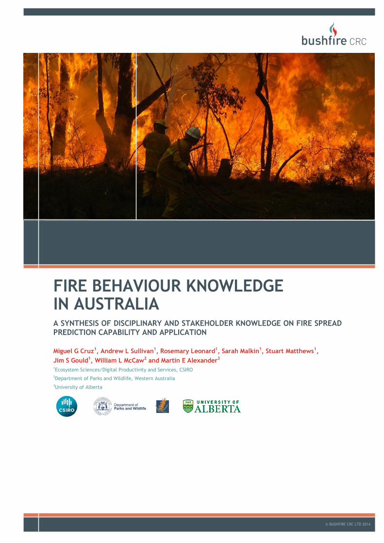
Firefighters battle to control a blaze. Photo by CFS Promotions Unit.
Citation:
Cruz, MG, Sullivan AL, Leonard, R, Malkin, S, Matthews, S, Gould JS,
McCaw, WL and Alexander, ME, (2014) Fire behaviour knowledge in
Australia, Bushfire CRC, Australia, ISBN: 978-0-9925684-2-9
Disclaimer:
CSIRO, the Department of Parks and Wildlife WA, the University of Alberta and the Bushfire Cooperative Research Centre advise that the information contained in this publication comprises general statements based on scientific research. The reader is advised and needs to be aware that such information may be incomplete or unable to be used in any specific situation. No reliance or actions must therefore be made on that information without seeking prior expert professional, scientific and technical advice. To the extent permitted by law, CSIRO, the
Department of Parks and Wildlife WA, the University of Alberta and the Bushfire Cooperative Research Centre (including its employees and consultants) exclude all liability to any person for any consequences, including but not limited to all losses, damages, costs, expenses and any other compensation, arising directly or indirectly from using this publication (in part or in whole) and any information or material contained in it.
Fire Behaviour Knowledge in Australia | i
Contents
Acknowledgments ............................................................................................................................................. iii
Executive summary............................................................................................................................................. v Fire Behaviour modelling review .......................................................................................................... v Fire Perimeter Propagation Software .................................................................................................. vi Current Fire Behaviour Analysts (FBAN) practice ............................................................................... vii
1 Introduction .......................................................................................................................................... 1
2 Australian fire spread prediction models: technical review ................................................................. 3 2.1 Introduction ................................................................................................................................ 3 2.2 Grasslands ................................................................................................................................... 8 2.3 Shrublands ................................................................................................................................ 21 2.4 Dry Eucalypt forests .................................................................................................................. 32 2.5 Wet Eucalypt forests ................................................................................................................. 47 2.6 Conifer plantations ................................................................................................................... 49 2.7 A list of fire behaviour models not reviewed in current study ................................................. 54 2.8 The Practice of Predicting Bushfire Behaviour ......................................................................... 55 2.9 Concluding remarks .................................................................................................................. 60
3 Fire Perimeter Propagation Modelling................................................................................................ 63 3.1 Introduction .............................................................................................................................. 63 3.2 Fire perimeter propagation methodologies ............................................................................. 63 3.3 Computational fluid dynamic modelling ................................................................................... 64 3.4 Computational fluid dynamics models ..................................................................................... 68 3.5 Simulation modelling ................................................................................................................ 76 3.6 Simulation models .................................................................................................................... 78 3.7 Operational evaluations ............................................................................................................ 86 3.8 Software development survey .................................................................................................. 87 3.9 Concluding remarks .................................................................................................................. 90
4 Fire Behaviour Analyst Practice: Survey and Interview ...................................................................... 93 4.1 Introduction .............................................................................................................................. 93 4.2 Method ..................................................................................................................................... 94 4.3 Results 1: The FBANs experience .............................................................................................. 97 4.4 Results 2: Major problems facing FBANs .................................................................................. 98 4.5 Results 3: Areas of confidence ................................................................................................ 110 4.6 Discussion ............................................................................................................................... 110 4.7 Concluding remarks ................................................................................................................ 113
5 References ......................................................................................................................................... 114
Appendix A Fire Simulation Software Developers Questionnaire ............................................................. 128
Appendix B FBAN Survey Results ............................................................................................................... 134

ii | Fire Behaviour Knowledge in Australia
Fire Behaviour Knowledge in Australia | iii
Acknowledgments
We would like to thank the following people and their organisations for the time and input into the project as our End User Group as well as providing feedback on the questions in the FBAN survey:
Mark Chladil (TFS), Gary Featherston (AFAC), Liam Fogarty (DEPI), Bruno Greimel (QRFS), Dylan Kendall (ACT PCS), Noreen Krusel (BCRC), Terry Maher (WA DPaW), Laurence McCoy (NSW RFS), Alen Slijepcevic (CFA) , Tim Wells (CFA), Mike Wouters (DEWNR).
We would also like to thank Gary Morgan (Bushfire CRC) for his enthusiasm and drive for this project.
Also, our thanks go to James Hilton and Lachlan Heatherton (CSIRO Computational Informatics) for their assistance in formulating the software developer’s survey questions, Wendy Anderson and Kelsey Gibos (Alberta Environment and Sustainable Resource Development) for feedback on the final report and to Dave Thomas (Renoveling, Ogden, Utah) for his comments on section 2.8.

iv | Fire Behaviour Knowledge in Australia
Fire Behaviour Knowledge in Australia | v
Executive summary
This project undertook a survey of the fire behaviour knowledge currently used by operational fire behaviour analysts (FBANs) in Australia and New Zealand for the purpose of predicting the behaviour and spread of bushfires. This included a review of the science, applicability and validation of current fire behaviour models, an examination of the fire perimeter propagation software currently being used by FBANs, and a survey of those FBANs to determine current work practices when carrying out fire behaviour predictions.
The objective of the work was to synthesise current operational fire behaviour knowledge and practice and to provide recommendations as to which fire behaviour models, supported by the science and defining operating bounds, should be used for operational prediction of fire spread. It is not a comprehensive review of all science related to fire behaviour.
While no single fire behaviour model will ever be perfect, the output of models that over-predict rate of spread can be easily readjusted whereas the output of models than under-predict rate of spread can have catastrophic consequences.
Fire Behaviour modelling review
• We conducted a technical review of existent fire spread models developed for Australian vegetation types, focusing on model functional forms, behaviour and published evaluation studies.
• This review allowed us to identify which models are the state-of-knowledge in fire behaviour science in Australia, and make recommendations as to which should underpin future fire behaviour prediction in Australia (see Table ES1).
• The review provides a scientific background in to which models used for operational fire behaviour prediction should be discontinued.
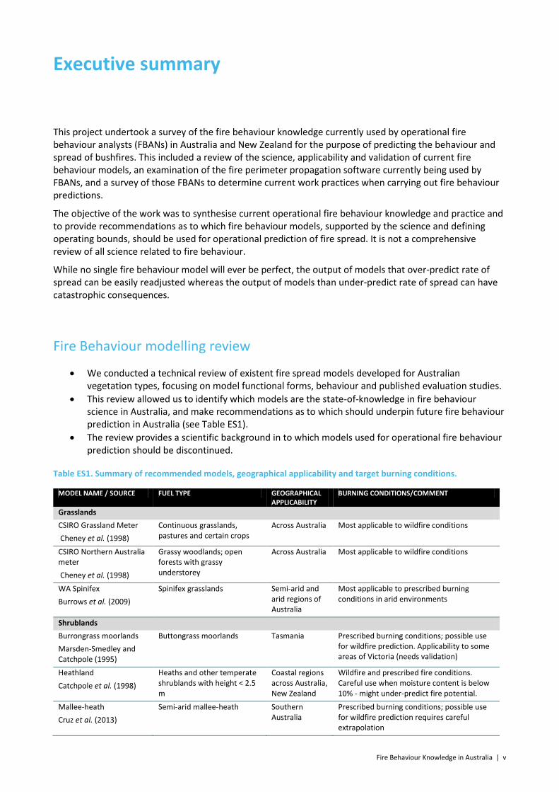
Table ES1. Summary of recommended models, geographical applicability and target burning conditions.
MODEL NAME / SOURCE FUEL TYPE GEOGRAPHICAL APPLICABILITY
BURNING CONDITIONS/COMMENT
Grasslands CSIRO Grassland Meter Cheney et al. (1998)
Continuous grasslands, pastures and certain crops
Across Australia Most applicable to wildfire conditions
CSIRO Northern Australia meter Cheney et al. (1998)
Grassy woodlands; open forests with grassy understorey
Across Australia Most applicable to wildfire conditions
WA Spinifex Burrows et al. (2009)
Spinifex grasslands Semi-arid and arid regions of Australia
Most applicable to prescribed burning conditions in arid environments
Shrublands Burrongrass moorlands Marsden-Smedley and Catchpole (1995)
Buttongrass moorlands Tasmania Prescribed burning conditions; possible use for wildfire prediction. Applicability to some areas of Victoria (needs validation)
Heathland Catchpole et al. (1998)
Heaths and other temperate shrublands with height < 2.5 m
Coastal regions across Australia, New Zealand
Wildfire and prescribed fire conditions. Careful use when moisture content is below 10% - might under-predict fire potential.
Mallee-heath Cruz et al. (2013)
Semi-arid mallee-heath Southern Australia
Prescribed burning conditions; possible use for wildfire prediction requires careful extrapolation
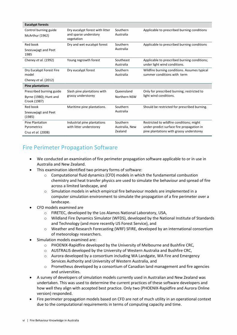
vi | Fire Behaviour Knowledge in Australia
Eucalypt forests Control burning guide McArthur (1962)
Dry eucalypt forest with litter and sparse understory vegetation
Southern Australia
Applicable to prescribed burning conditions
Red book Sneeuwjagt and Peet 1985
Dry and wet eucalypt forest Southern Australia
Applicable to prescribed burning conditions
Cheney et al. (1992) Young regrowth forest Southeast Australia
Applicable to prescribed burning conditions; under light wind conditions.
Dry Eucalypt Forest Fire model Cheney et al. (2012)
Dry eucalypt forest Southern Australia
Wildfire burning conditions. Assumes typical summer conditions with term
Pine plantations Prescribed burning guide Byrne (1980); Hunt and Crook (1987)
Slash pine plantations with grassy understorey
Queensland Northern NSW
Only for prescribed burning; restricted to light wind conditions.
Red book Sneeuwjagt and Peet (1985)
Maritime pine plantations. Southern Australia
Should be restricted for prescribed burning.
Pine Plantation Pyrometrics Cruz et al. (2008)
Industrial pine plantations with litter understorey
Southern Australia, New Zealand
Restricted to wildfire conditions; might under-predict surface fire propagation in pine plantations with grassy understorey
Fire Perimeter Propagation Software
• We conducted an examination of fire perimeter propagation software applicable to or in use in Australia and New Zealand.
• This examination identified two primary forms of software: o Computational fluid dynamics (CFD) models in which the fundamental combustion
chemistry and heat transfer physics are used to simulate the behaviour and spread of fire across a limited landscape, and
o Simulation models in which empirical fire behaviour models are implemented in a computer simulation environment to simulate the propagation of a fire perimeter over a landscape.
• CFD models examined are o FIRETEC, developed by the Los Alamos National Laboratory, USA, o Wildland Fire Dynamics Simulator (WFDS), developed by the National Institute of Standards
and Technology (and more recently US Forest Service), and o Weather and Research Forecasting (WRF) SFIRE, developed by an international consortium
of meteorology researchers. • Simulation models examined are:
o PHOENIX-Rapidfire developed by the University of Melbourne and Bushfire CRC, o AUSTRALIS developed by the University of Western Australia and Bushfire CRC, o Aurora developed by a consortium including WA Landgate, WA Fire and Emergency
Services Authority and University of Western Australia, and o Prometheus developed by a consortium of Canadian land management and fire agencies
and universities. • A survey of developers of simulation models currently used in Australian and New Zealand was
undertaken. This was used to determine the current practices of these software developers and how well they align with accepted best practice. Only two (PHOENIX-Rapidfire and Aurora Online version) responded.
• Fire perimeter propagation models based on CFD are not of much utility in an operational context due to the computational requirements in terms of computing capacity and time.

Fire Behaviour Knowledge in Australia | vii
• Simulation models based on existing empirical models of fire behaviour and methods for applying them spatially have been shown to be of potentially significant assistance to an FBAN.
• The quality of a fire simulation prediction is highly dependent upon the quality of the data used to obtain it. Thus it is very difficult to quantify the reasons for simulator performance given the large number of variables and spatial and temporal variation in those variables during the period of active fire spread.
• Prometheus, an implementation of the Canadian Forest Fire Behaviour Prediction System (and available in a version suitable for use in New Zealand), does not contain fuel types applicable to Australian native forest or shrubland fuel types. Furthermore, under extreme fire weather conditions in Australia the fire behaviour models for conifer plantation (C-6) and grasslands (O-1) are likely to significantly under-predict (by more than 50%) the maximum forward rate of spread in these fuel types. As a result, Prometheus is not recommended for use in Australian conditions.
• Without conducting a detailed comparison of the performance of the remaining models in regard to quality of fire spread simulation (which was beyond the scope of this project given the limitations in time and budget), the choice of selection of which model is most suited to fire behaviour prediction will be driven by consideration of software licensing and data requirements, development pathways and software maintenance, software support and useability, and interoperability needs of the user organisation.
• In order to determine suitability of fire simulation models it is suggested that extensive testing of possible models against a set of well-documented fire events across a broad range of burning and fuel conditions be undertaken by an independent assessment team utilising the range of performance metrics developed for such purposes.
• It is further suggested that such comparisons of performance be carried out regularly as a form of independent testing of such models as they are continuously developed and improved.
Current Fire Behaviour Analysts (FBAN) practice
The recent and rapid developments in diverse fire behaviour analysis techniques have led to a need for:
1. more, and more highly trained fire behaviour analysts (FBANs),
2. greater understanding of the available technologies,
3. reconsideration of the organisational support, positioning and deployment of FBANs,
4. a review of current specialist FBAN practices and requirements for assisting them to improve their performance.
The research addressed the fourth issue: A review of current specialist FBAN practices and the requirements for assisting them to improve their performance.
A detailed and lengthy online survey of 101 questions was developed to cover FBANs background, training prediction processes, fire prediction tools and simulation models, data inputs, outputs and review of their fire predictions. Thirty-two FBANs from all six Australian states and New Zealand responded and six gave follow up interviews. They were all experienced FBANs with a minimum of two years experience in the role and had undertaken predictions for at least two major fires.
The survey was informed by the CSIRO fire behaviour experts managing other tasks in the project and an expert panel consisting of ten senior fire managers from New South Wales, Victoria, Tasmania, Western Australia, South Australia, Australian Capital Territory, and New Zealand.
The results showed that nearly half the FBANs rated the adequacy of their prediction process as fair or poor and identified a number of areas where the role of the FBAN could be better supported:
• More reliable local inputs: Predictions would be improved with more reliable local inputs, especially for fuel load. Wind speed and direction were also problematic. Only six FBANs usually had access to

viii | Fire Behaviour Knowledge in Australia
the fire site themselves and one mentioned a trained ground observer. For the others, access to local data seemed to be rather ad hoc.
• Accessing online systems and databases: Pre-season updates were needed to familiarise FBANs with any new systems; access to fire authority systems for FBANs from other departments; ensuring regional areas are properly resourced were all improvements that could be addressed.
• Better communication with the incident management team: Better education of IMT leaders was seen as key for the FBANs to obtain the feedback they need and for their predictions to be properly interpreted. However FBAN outputs seem to be quite variable and more standardised products might be easier for educating IMT leaders.
• Further training: Although all the FBANs used a range of informal systems for updating their skills (e.g. reading case studies, reading research, online groups) there was a need for more formal courses to increase their skills and keep them up to date with technical developments.
• A need for more opportunities to gain experience and feedback: Some FBANs lacked regular assignments partly because extra FBANs are called in when the regulars are too busy, that is when the fire situation is severe. This creates an inverse relationship between the size of the fire problem and experience of FBANs which does not seem ideal. There was a general lack of regular feedback on their predictions suggesting the need for feedback systems to be put in place.
• Complexity of managing inputs and predictions from numerous tools: To a certain extent a variety of tools is desirable to deal with differing local conditions and to validate predictions by comparisons across methods. However, there were a very large number of tools that FBANs used occasionally making it difficult for them to become expert in the strengths, weaknesses, and assumptions of them all. The FBANs’ work could be simplified by further development and validation of a selection of tools so they can be used with confidence.
• Areas of confidence: Despite these issues noted above, FBANs reported being confident in a number of areas, particularly in the models they commonly used and providing predictions to the incident management teams in a timely way.
Rapid advances in fire prediction technologies have greatly increased the effectiveness and the specialisation of fire behaviour analysis. As with most times of rapid change there is a need for reflection, integration, and validation. There is also a need to adjust organisational systems, roles and training to maximise the benefits. Rectifying the problems identified by appears quite manageable and a worthwhile investment given the lives and property that are at stake.
Fire Behaviour Knowledge in Australia | 1
1 Introduction
Good knowledge of expected bushfire behaviour is essential for a number of critical tasks across the Prevention-Planning-Response-Recovery (PPRR) disaster management cycle. It is essential to understand the level of risk posed by bushfires in any particular area, to identify steps that may be taken to mitigate the occurrence and impact of bushfires, to identify the level of protection required for town planning and urban design standards, to inform hazard reduction planning and suppression preparedness, and it is essential for responding to bushfire outbreaks.
The role of Fire Behaviour Analyst (FBAN) has grown in recent years to be a key component in the planning sections of most Incident Management Teams put in place to undertake emergency response actions to wildfire and other incidents (Slijepcevic et al. 2008). The primary tools of the FBAN have been and will continue to be experience and knowledge of fire behaviour but increasingly the demands of the role have required reliance upon formalised fire behaviour knowledge in the form of mathematical models of fire behaviour in a range of fuel types.
This increasing demand is driven by a number of factors but primary amongst them is the need for an FBAN to carry out predictions for multiple fire events with short deadlines for localities in which their inherent localised fire behaviour knowledge is limited or non-existent. The reliance, then upon robust and reliable fire behaviour models to predict likely rates of forward spread, spotting distance, flame heights, etc, becomes critical.
Understanding which fire behaviour models are best to use for the prevailing fuel, weather and topographic conditions, what the limitations of the individual models are, and, probably most importantly, knowing when a particular fire behaviour model should not be used, is paramount.
It should be clearly noted that the focus of this work is fire behaviour, not fire danger. Current systems for determining the level of fire danger are distinctly different from those used for determining potential fire behaviour and should not be confused. Determination of level of fire danger is carried out by the Bureau of Meteorology and the state rural fire authority and is done so according to various pieces of state legislation. The determination of expected fire behaviour, however, is not covered by state legislation and is carried out as needed.
The Bushfire CRC initiated this project, the Bushfire Behaviour Knowledge Synthesis project, with primary purpose of collating all existing operational fire behaviour knowledge relevant to Australian and New Zealand fire conditions into one place and assessing the performance of each from a science perspective to determine those that should be recommended for use, along with the recommended conditions for use, and those that should not be used.
While previous studies of this sort have been done in the past (e.g. Cook et al. 2009), they have generally been specific to a given jurisdiction and not applicable to the nation as a whole. Furthermore, it was understood that a literal harvest of the literature in regard to published fire behaviour models would not be the complete story of operational fire behaviour prediction. To augment the literature review of relevant fire models, the opportunity was taken to survey FBAN practitioners across Australasia to find out how the service of fire behaviour prediction was carried out operationally. To that end each jurisdiction identified core FBANs within their ranks to participate in the survey.
A further component of the project was a broad assessment of the operational fire perimeter propagation prediction software currently in use across Australasia. The results of the FBAN survey informed the coverage of the software assessment and subsequent software developer survey. This survey was undertaken to gather information about the nature of the fire perimeter propagation prediction software

2 | Fire Behaviour Knowledge in Australia
currently in operational use in Australasia and the software engineering practises employed to develop, maintain and improve this software.
This project has direct synergies with and is complementary to the concurrent AFAC Rural and Land Managers Group Predictive Services-User Requirements project with this project providing the core science and operational understanding of the primary tools of fire spread prediction.
Fire Behaviour Knowledge in Australia | 3
2 Australian fire spread prediction models: technical review
2.1 Introduction
Foley (1947) provides a comprehensive account of the semi-quantitative methods of assessing bushfire potential used in Australia up to the late 1940’s. Models of fire behaviour are now widely used operationally to assess current fire situations, to assess future scenarios and especially to evaluate of alternative wildland fire management strategies. The outputs of these models − e.g. rate of fire spread, flame height and fire intensity− are important for both fire management and research applications in areas such as suppression strategies, public and fire-fighter safety, short- and long-term fire ecology/fire impacts, smoke emission and protection of the wildland urban interface (Cruz and Gould 2009). As Underwood (1985) notes, “The management or control of forest fires in Australia will never become a reality until the behaviour of fires can be predicting accurately over the many conditions under which they occur.”
Over the years the development of fire behaviour models have taken on two broad approaches (Van Wagner 1971): (i) physical or semi (or quasi) - physical models based on the fundamental processes driving fire propagation, and (ii) empirical or semi-empirical models based on statistical methods (Weber 1991, Pastor et al. 2003, Sullivan 2009a and b). The former have generally taken the form of complex numerical codes related to solutions of the Navier-Stokes equations for the motion of fluid. The latter have generally been simple analytical functions relating key dependent variables such as fire rate of forward spread with key independent variables such as wind speed or fuel conditions.
Both modelling approaches have advantages and disadvantages for various purposes, but due to their relative computation simplicity and ease of use, only the empirical and quasi-empirical approaches have produced working models that have been used operationally (Sullivan 2009c).
Since the pioneering outdoor experimental burning work by Alan G. McArthur and George B. Peet beginning in the early 1950’s and early 1960’s (McArthur 1962, 1967; McArthur and Luke 1963; Peet 1965), a considerable number of similar field-based studies carried out in Australia have extended our understanding of fire behaviour in a variety of fuel types (e.g., Cheney et al. 1993; McCaw et al. 2012; Cheney et al. 2012). Models have been developed through time (Fig. 2.1) with the aim of
1. describing fire behaviour in a fuel type where such knowledge did not exist or 2. replacing a model that has been found to not perform adequately under certain conditions.
Unlike the approach taken in the US for fire behaviour model development, and similar to that taken in Canada, Australian fire behaviour models have been fuel type specific. That is, models are developed for a particular fuel type and cannot reasonably be applied to another fuel type characterized by a distinct fuel structure. If a model is needed for an additional fuel type, new experiments in that fuel type are required to document and quantify fire behaviour.
Over the years fire behaviour models have been made available to users in a number of different forms, ranging from numerical tables, slide rules, technical reports, through to analytical equations, published journals, etc. Early versions of models by the likes of McArthur and Peet were presented as tables and slide rules. These were later transformed into equations (e.g. Noble et al. 1980; Beck 1995) which then lead to software applications (e.g., Crane 1982) that greatly increased their utility (with perhaps a loss of understanding of how the systems actually worked).
While various summaries have been published (Cheney 1981; Catchpole 2002; Sullivan et al. 2012) no single document has yet described the full extent of the fire behaviour modelling knowledge developed in Australia to date. Furthermore, it is observed that in some instances outdated and superseded models
4 | Fire Behaviour Knowledge in Australia
continue to be used by fire management agencies for a number of reasons. These include lack of adequate training materials with clear information on the limitations of the older models or insufficient data on distinct input parameters required for the newer models. This situation coupled with the distinct modelling frameworks, which are a reflection of the individual modeller’s view of the system, has created a case where it is now not clear to users of these models, the underlying assumptions and limitations, and in particular the limits of applicability of a given model.
The objective of the present contribution is to provide in a single document a description of the various models used operationally in Australia to predict bushfire rate of spread and, when applicable, fire sustainability. To give users a better understanding of each model and their application bounds we provide the mathematical equations that form each model and a brief description of data used in model development. We also discuss the main input variables and their influence in the model and report on known published evaluation studies.
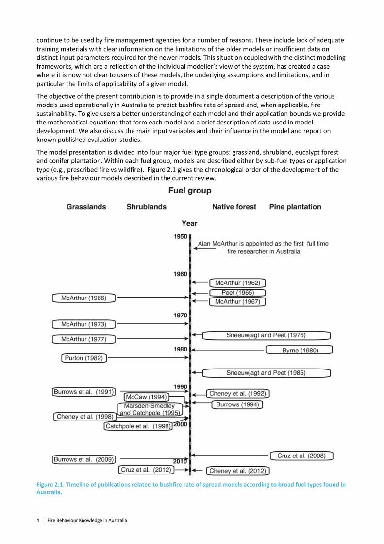
The model presentation is divided into four major fuel type groups: grassland, shrubland, eucalypt forest and conifer plantation. Within each fuel group, models are described either by sub-fuel types or application type (e.g., prescribed fire vs wildfire). Figure 2.1 gives the chronological order of the development of the various fire behaviour models described in the current review.
Figure 2.1. Timeline of publications related to bushfire rate of spread models according to broad fuel types found in Australia.
Fire Behaviour Knowledge in Australia | 5
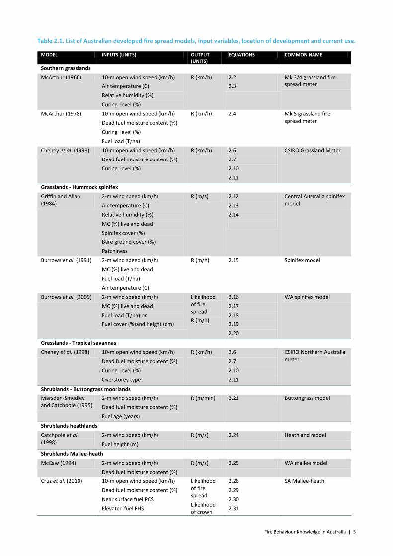
Table 2.1. List of Australian developed fire spread models, input variables, location of development and current use.
MODEL INPUTS (UNITS) OUTPUT (UNITS)
EQUATIONS COMMON NAME
Southern grasslands McArthur (1966) 10-m open wind speed (km/h)
Air temperature (C) Relative humidity (%) Curing level (%)
R (km/h) 2.2 2.3
Mk 3/4 grassland fire spread meter
McArthur (1978) 10-m open wind speed (km/h) Dead fuel moisture content (%) Curing level (%) Fuel load (T/ha)
R (km/h) 2.4 Mk 5 grassland fire spread meter
Cheney et al. (1998) 10-m open wind speed (km/h) Dead fuel moisture content (%) Curing level (%)
R (km/h) 2.6 2.7 2.10 2.11
CSIRO Grassland Meter
Grasslands - Hummock spinifex Griffin and Allan (1984)
2-m wind speed (km/h) Air temperature (C) Relative humidity (%) MC (%) live and dead Spinifex cover (%) Bare ground cover (%) Patchiness
R (m/s) 2.12 2.13 2.14
Central Australia spinifex model
Burrows et al. (1991) 2-m wind speed (km/h) MC (%) live and dead Fuel load (T/ha) Air temperature (C)
R (m/h) 2.15
Spinifex model
Burrows et al. (2009) 2-m wind speed (km/h) MC (%) live and dead Fuel load (T/ha) or Fuel cover (%)and height (cm)
Likelihood of fire spread R (m/h)
2.16 2.17 2.18 2.19 2.20
WA spinifex model
Grasslands - Tropical savannas Cheney et al. (1998) 10-m open wind speed (km/h)
Dead fuel moisture content (%) Curing level (%) Overstorey type
R (km/h) 2.6 2.7 2.10 2.11
CSIRO Northern Australia meter
Shrublands - Buttongrass moorlands Marsden-Smedley and Catchpole (1995)
2-m wind speed (km/h) Dead fuel moisture content (%) Fuel age (years)
R (m/min) 2.21 Buttongrass model
Shrublands heathlands Catchpole et al. (1998)
2-m wind speed (km/h) Fuel height (m)
R (m/s) 2.24 Heathland model
Shrublands Mallee-heath McCaw (1994) 2-m wind speed (km/h)
Dead fuel moisture content (%) R (m/s) 2.25 WA mallee model
Cruz et al. (2010) 10-m open wind speed (km/h) Dead fuel moisture content (%) Near surface fuel PCS Elevated fuel FHS
Likelihood of fire spread Likelihood of crown
2.26 2.29 2.30 2.31
SA Mallee-heath

6 | Fire Behaviour Knowledge in Australia
Overstorey Height (%) fire spread R (m/min)
2.32
Cruz et al. (2013) 10-m open wind speed (km/h) Dead fuel moisture content (%) Overstorey Cover (%) Overstorey Height (%)
Likelihood of fire spread Likelihood of crown fire spread R (m/min)
2.33 2.34 2.35 2.36 2.37
Mallee-heath
Dry eucalypt forests – prescribed burning McArthur (1962) 1.5-m wind speed (km/h)
Dead fuel moisture content (%) Fuel load (T/ha)
R (m/min) 2.38 2.39 2.40
Leaflet 80; Control burning guide
Sneeuwjagt and Peet (1985)
2-m wind speed (km/h) Dead fuel moisture content (%) Fuel load (T/ha)
R (m/h) 2.46 2.47 2.48 2.50-53 2.54
Red book; Forest Fire Behaviour Tables
Cheney et al. (1992) 2-m wind speed (km/h) Dead fuel moisture content (%) Near-surface fuel height (m)
R (m/min) 2.55
Dry eucalypt forests – wildfire McArthur (1967) 10-m open wind speed (km/h)
Air temperature (C) Relative humidity (%) Drought factor KBDI Time since rain Last rain amount Available litter fuel load
R (km/h) 2.56 2.57 2.64
Mk 5 Forest Fire Danger Meter
Cheney et al. (2012) 10-m open wind speed (km/h) Dead fuel moisture content (%) Surface FHS Near-surface FHS Near-surface fuel height (cm)
R (m/h) 2.65 2.66 2.68
Dry Eucalypt Forest Fire model Vesta model
Wet eucalypt forests – prescribed burning Sneeuwjagt and Peet (1985)
2-m wind speed (km/h) Dead fuel moisture content (%) Fuel load (T/ha)
R (m/h) 2.69 2.70 2.71 2.72 2.73-76 2.77
Red book; Forest Fire Behaviour Tables
Pine plantations – prescribed burning Byrne (1980); Hunt and Crook (1987)
10-m open wind speed (km/h) Relative humidity (%) Available understorey fuel load
R (m/h) 2.78 Prescribed burning guide Mk 3
Sneeuwjagt and Peet (1985)
2-m wind speed (km/h) Dead fuel moisture content (%) Fuel load (T/ha)
R (m/h) See 2.46-2.54 2.79 2.80
Red book; Forest Fire Behaviour Tables
Pine plantations – wildfire Cruz et al. (2008) 10-m openwind speed (km/h)
Air temperature (%) Fine dead fuel moisture content
R (m/h) Fire type
PPPY – Pine Plantation Pyrometrics
Fire Behaviour Knowledge in Australia | 7
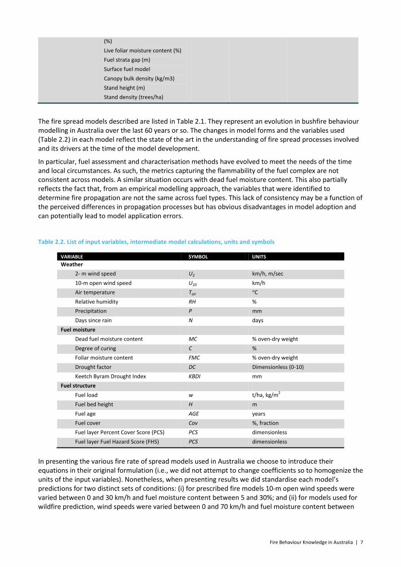
(%) Live foliar moisture content (%) Fuel strata gap (m) Surface fuel model Canopy bulk density (kg/m3) Stand height (m) Stand density (trees/ha)
The fire spread models described are listed in Table 2.1. They represent an evolution in bushfire behaviour modelling in Australia over the last 60 years or so. The changes in model forms and the variables used (Table 2.2) in each model reflect the state of the art in the understanding of fire spread processes involved and its drivers at the time of the model development.
In particular, fuel assessment and characterisation methods have evolved to meet the needs of the time and local circumstances. As such, the metrics capturing the flammability of the fuel complex are not consistent across models. A similar situation occurs with dead fuel moisture content. This also partially reflects the fact that, from an empirical modelling approach, the variables that were identified to determine fire propagation are not the same across fuel types. This lack of consistency may be a function of the perceived differences in propagation processes but has obvious disadvantages in model adoption and can potentially lead to model application errors.
Table 2.2. List of input variables, intermediate model calculations, units and symbols
VARIABLE SYMBOL UNITS Weather
2- m wind speed U2 km/h, m/sec 10-m open wind speed U10 km/h Air temperature Tair °C Relative humidity RH % Precipitation P mm Days since rain N days
Fuel moisture Dead fuel moisture content MC % oven-dry weight Degree of curing C % Foliar moisture content FMC % oven-dry weight Drought factor DC Dimensionless (0-10) Keetch Byram Drought Index KBDI mm
Fuel structure Fuel load w t/ha, kg/m2 Fuel bed height H m Fuel age AGE years Fuel cover Cov %, fraction Fuel layer Percent Cover Score (PCS) PCS dimensionless Fuel layer Fuel Hazard Score (FHS) PCS dimensionless
In presenting the various fire rate of spread models used in Australia we choose to introduce their equations in their original formulation (i.e., we did not attempt to change coefficients so to homogenize the units of the input variables). Nonetheless, when presenting results we did standardise each model’s predictions for two distinct sets of conditions: (i) for prescribed fire models 10-m open wind speeds were varied between 0 and 30 km/h and fuel moisture content between 5 and 30%; and (ii) for models used for wildfire prediction, wind speeds were varied between 0 and 70 km/h and fuel moisture content between
8 | Fire Behaviour Knowledge in Australia
2.5 and 12.5%. Irrespective of the original model output values, rates of fire spread are given in m/min. Fireline intensities quoted within this section of the document follow Byram (1959).
Slope is a variable with a dramatic effect on fire propagation. Fires spreading in positive slopes aligned with the wind are known to increase their rate of spread several fold (Viegas 2004). All but one of the model formulations described in the present paper calculate the rate of spread for flat ground in which topographic slope is not present and then use a common slope correction factor such as presented by McArthur (1962) for forest fuel types, to convert to a slope-affected rate of spread. The McArthur’s (1967) rate of fire spread slope function is (from Noble et al. 1980):
𝑅𝜃 = 𝑅 × exp (0.069 × 𝜃) [2.1]
Where Rθ is the rate of fire spread on given slope, θ is the slope angle in degrees and R the calculated rate of fire spread for flat ground. This equation should be restricted to the application bounds 0 < θ < 20 degrees. Recent work has suggested that the negative slope correction factor should not exceed 0.5 of R (Sullivan et al. in review).
One of the issues of this slope effect is that McArthur function is not intended to describe the sole mechanical effect of slope in fire propagation, as it is normally achieved in a laboratory setting, but to incorporate broad topographic convergence associated with slope (e.g., increase wind speed near ridge tops, drier fuels, etc). Its accurate use requires a judicious understanding of the local conditions the fire is spreading. McArthur(1967) recommends the function to be most applicable to fires burning under milder conditions or going through their build-up stage. For large wildfires burning over multiple watersheds the effect of slope on the overall rate of spread can be disregarded (McArthur 1967; Rothermel 1991).
2.2 Grasslands
Grass represents the most widespread fuel type in Australia (Moore 1970). The diversity of species and climates where grass fuels are distributed results in a number of distinct fuel groups which for fire behaviour prediction purposes are typified as (i) southern grasslands (ii) hummock spinifex grasslands; and (iii) tropical grasslands, woodlands and open forests (Cheney and Sullivan 2008). In many cases, grasslands are not homogeneous but often co-located with other vegetation such as found in savannah grasslands, woodlands and open forests. In each of these, if grass is the dominant understorey vegetation it is considered a grassland fuel (Sullivan et al. 2012).
2.2.1 SOUTHERN GRASSLANDS
McArthur Grassland Fire Danger Meters
Model description
Alan G. McArthur published the first results of research into grassland fire danger and fire behaviour as a set of tables that quantified grassland fire danger and related categories of expected fire behaviour (McArthur 1960). He continued development of this knowledge in the form of cardboard slide rules, the Grassland Fire Danger Meters. These meters incorporated the effects of weather and fuel conditions on a fire danger index and rate of fire spread in grassland pastures. The meters were deemed applicable to annual grasslands of fine structure in the temperate regions of Australia. They were designed to be used in the field and the office by fire managers using actual or forecast weather conditions and observations of fuel state.
At the foundation of the meters were datasets collected from well-documented wildfires and a number of experimental fires (Luke and McArthur 1978). The Forestry and Timber Bureau program of experimental burning and wildfire documentation in grasslands lasted for several decades (e.g. Forest and Timber Bureau 1960, 1970), with new insights into fire behaviour leading to updates in the meters. The meters were originally not developed as equations but published as slide rules, either straight (e.g., Mk 1, Mk 2 and Mk 5) or circular (Mk 3 and 4).
Fire Behaviour Knowledge in Australia | 9
The first version of the grassland fire danger meter incorporated the effects of air temperature, relative humidity, wind speed, fuel curing and fuel load and provided an estimate of the rate of forward spread of the fire, flame height and Grassland Fire Danger Index (GFDI). Rate of fire spread was directly related to the GFDI. A modified version of this meter was published in 1962 (Cheney pers. comm.). Both these meters were expressed in imperial units. No equations exist to describe the functional forms imbedded in these meters.
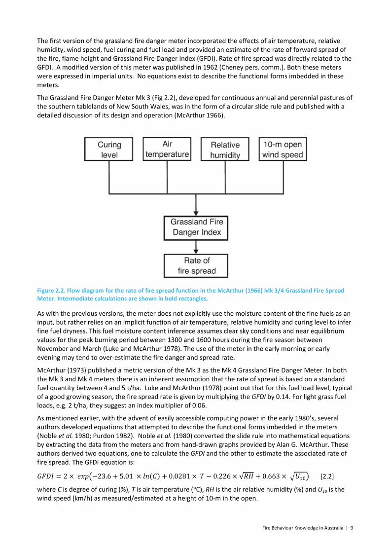
The Grassland Fire Danger Meter Mk 3 (Fig 2.2), developed for continuous annual and perennial pastures of the southern tablelands of New South Wales, was in the form of a circular slide rule and published with a detailed discussion of its design and operation (McArthur 1966).
Figure 2.2. Flow diagram for the rate of fire spread function in the McArthur (1966) Mk 3/4 Grassland Fire Spread Meter. Intermediate calculations are shown in bold rectangles.
As with the previous versions, the meter does not explicitly use the moisture content of the fine fuels as an input, but rather relies on an implicit function of air temperature, relative humidity and curing level to infer fine fuel dryness. This fuel moisture content inference assumes clear sky conditions and near equilibrium values for the peak burning period between 1300 and 1600 hours during the fire season between November and March (Luke and McArthur 1978). The use of the meter in the early morning or early evening may tend to over-estimate the fire danger and spread rate.
McArthur (1973) published a metric version of the Mk 3 as the Mk 4 Grassland Fire Danger Meter. In both the Mk 3 and Mk 4 meters there is an inherent assumption that the rate of spread is based on a standard fuel quantity between 4 and 5 t/ha. Luke and McArthur (1978) point out that for this fuel load level, typical of a good growing season, the fire spread rate is given by multiplying the GFDI by 0.14. For light grass fuel loads, e.g. 2 t/ha, they suggest an index multiplier of 0.06.
As mentioned earlier, with the advent of easily accessible computing power in the early 1980’s, several authors developed equations that attempted to describe the functional forms imbedded in the meters (Noble et al. 1980; Purdon 1982). Noble et al. (1980) converted the slide rule into mathematical equations by extracting the data from the meters and from hand-drawn graphs provided by Alan G. McArthur. These authors derived two equations, one to calculate the GFDI and the other to estimate the associated rate of fire spread. The GFDI equation is:
𝐺𝐹𝐷𝐼 = 2 × 𝑒𝑥𝑝�−23.6 + 5.01 × 𝑙𝑛(𝐶) + 0.0281 × 𝑇 − 0.226 × √𝑅𝐻 + 0.663 × �𝑈10� [2.2]
where C is degree of curing (%), T is air temperature (°C), RH is the air relative humidity (%) and U10 is the wind speed (km/h) as measured/estimated at a height of 10-m in the open.

10 | Fire Behaviour Knowledge in Australia
The headfire rate of spread in km/h is then calculated as:
𝑅 = 0.13 × 𝐺𝐹𝐷𝐼 [2.3]
It is important to note that in the process of deriving the equations from data extracted from the meters there occur slight differences between the two methods, normally less than 2% This might explain the slight difference between the 0.13 factor in Eq. 2.3 and the 0.14 factor as suggested by Luke and McArthur (1978).
Evidence from the 1977 fires in the Western District of Victoria (McArthur et al. 1982) suggested to McArthur a need to reincorporate the fuel load effect (present in the Mk 1 and Mk 2 meters) in the GFDI and grassfire rate of spread in order to improve the rate of spread prediction in eaten-out pastures. The Mk 5 meter was published as a rectangular slide rule meter in 1978 by the Country Fire Authority, Victoria (McArthur 1978). Changes from the Mk3/Mk4 versions of the grassland fire danger meter include the implicit effect of fuel load on GFDI and rate of spread, the addition of fuel moisture content as an explicit component predicted from air temperature and relative humidity (Fig 2.3) and a modified wind function. The slide rule meter was formulated to have fuel load input varying between 1 and 6 t/ha. Fuel moisture content for partially cured grasslands is considered to be an aggregate of live and dead fuels.
As per the Mk 3/4 grassland fire danger meter, Noble et al. (1980) converted the data extracted from the Mk 5 slide rule into an equation. The extracted data suggested a stepwise GFDI equation with the effect of fuel moisture content changing below an 18.8% threshold:
𝐺𝐹𝐷𝐼 = �3.35 × 𝑤 × 𝑒𝑥𝑝(−0.0897 × 𝑀𝐶 + 0.0403 × 𝑈10) 𝑀𝐶 < 18.8%
0.299 × 𝑤 × 𝑒𝑥𝑝(−1.686 + 0.0403 × 𝑈10) × (30−𝑀𝐶) 30 ≥ 𝑀𝐶 ≥ 18.8%
�
[2.4]
The moisture content (MC) of the grassland fuel is also considered to be an aggregate of live and dead fuels. The MC equation was derived as:
𝑀𝐶 = (97.7+4.06×𝑅𝐻)(𝑇+6) − 0.00854 × 𝑅𝐻 + 3000
𝐶− 30 [2.5]
At a curing level less than approximately 50%, Eq. 2.5 predicts an overall fuel moisture above 30%, the moisture of extinction implicit in Eq. 2.4. For the Mk 5 meter the rate of spread is derived from the GFDI (Eq. 2.4) as per the Mk 3 meter (Eq. 2.3).
Figure 2.3. Flow diagram for the rate of fire spread function in the McArthur (1978) Mk 5 Grassland Fire Spread Meter. Intermediate calculations are shown in bold rectangles.
Fire Behaviour Knowledge in Australia | 11
Purdon (1982) assumed that the Mk 5 fuel load function could be extrapolated into the Mk 4 meter, which at that time was still used operationally for determining GFDI. This author also suggested that the Mk 4 was not a direct metric conversion of the Mk 3 meter. By determining the relationship between the angular variation in the meters and the fire danger index value he points out that the Mk 4 meter indices are lower than those obtained in the Mk 3 version of the meter by about 10%. It is likely, however, that these discrepancies arise from the methods used to extract the data from highly variable cardboard meters rather than a reformulation of the GFDI function.
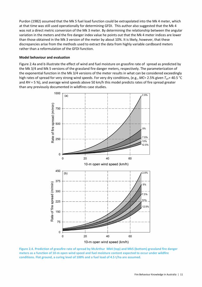
Model behaviour and evaluation
Figure 2.4a and b illustrate the effect of wind and fuel moisture on grassfire rate of spread as predicted by the Mk 3/4 and Mk 5 versions of the grassland fire danger meters, respectively. The parameterization of the exponential function in the Mk 3/4 versions of the meter results in what can be considered exceedingly high rates of spread for very strong wind speeds. For very dry conditions, (e.g., MC= 2.5% given Tair= 40.5 °C and RH = 5 %), and average wind speeds above 50 km/h this model predicts rates of fire spread greater than any previously documented in wildfires case studies.
Figure 2.4. Prediction of grassfire rate of spread by McArthur Mk4 (top) and Mk5 (bottom) grassland fire danger meters as a function of 10-m open wind speed and fuel moisture content expected to occur under wildfire conditions. Flat ground, a curing level of 100% and a fuel load of 4.5 t/ha are assumed.

12 | Fire Behaviour Knowledge in Australia
For the same level of fuel dryness, the predicted rate of spread exceeds the wind speed when the latter variable is above approximately 80 km/h. It is unknown if this unreasonable behaviour for extreme conditions is a result of the original McArthur formulation or due to the parameterization chosen by Noble et al. (1980). The effect of wind speed in the Mk 5 meter is significantly lower than observed in the Mk 3/4. Fuel moisture content is also observed to be distinctly different in the two meters, with the Mk 3/4 showing a higher effect than the Mk. 5.
The effect of grassland curing on rate of fire spread is also quite different between the various versions of the grassland fire danger meters, with the Mk 3/4 versions incorporating an exponential function while the Mk 5 function is more linear in nature. The effect of curing is more marked in the Mk 3/4 meter.
The Mk 3/4 does not incorporate the effect of fuel load on rate of fire spread as such, however, as mentioned previously, Luke and McArthur (1978) provide two rate of spread factors to convert GFDI into rate of fire spread, namely 0.14 for improved grasslands with a fuel load between 4 and 5 t/ha and 0.06 for lighter load grasslands of approximately 2 t/ha. This suggests a direct fuel load effect -- i.e., a doubling of the fuel load will lead to a doubling in the rate of fire spread. This is the function that is implemented in the Mk 5 meter. Nonetheless, this correction factor is considered questionable, as there are confounding effects as a result of fuel particle size (Luke and McArthur 1978). Fine grasses will normally carry lighter fuel loads, although their fineness will contribute to higher spread rates. Later studies (see Cheney et al. (1998) below) showed this fuel load effect on the rate of fire spread to be much smaller than that given by the Mk 5.
Kilinc et al. (in press) evaluated the performance of the Mk3/4 and Mk 5 meters against wildfire data (n=187) from southern Australia. This dataset comprised mostly fires in grazed and eaten-out pastures with the fire rate of spread varying between 1.7 to 560 m/min. The Mk 3/4 meters predicted the dataset with an average absolute error of 95 m/min (124% mean error) and an average over-prediction bias of 65 m/min. The Mk 5 meter on the other hand assuming arbitrary standardized fuel load (e.g., 2.5 t/ha for grazed pastures) performed considerably better with an average absolute error of 64 m/min (51% mean error) and an average under-prediction bias of 40 m/min.
CSIRO Grassland Fire Spread Model (Cheney et al. 1998)
Model description
Cheney et al. (1993) detailed an experimental burning project in the Northern Territory of Australia, to determine the relative importance of grass fuel characteristics and fire size on the rate of spread of grassfires. This work grew out of the confusion seeded by the introduction of the Mk 5 GFDM prior to McArthur’s death in 1978 and the different GFDI calculated by the different meters, and the question of the true effect of fuel load on rate of fire spread.
A total of 121 experimental fires were conducted during July and August of 1986 at the Annaburroo Station (12o34′40″S, 131o09′20″E) in open grassland. Fuels were treated to change fuel load, fuel height and a combination of these. In this dataset the rate of fire spread varied from 17.4 to 117 m/min, 2-m wind speed between 7 and 25 km/h, air temperatures from 23 to 33°C, and relative humidity from 23 to 45%. Using this dataset and data from wildfire case studies (n=20) Cheney et al. (1998) developed an empirical model for predicting the rate of spread of grassland fires in undisturbed (Rn, m/min) and cut/grazed (Rcu, m/min) pastures:
𝑅𝑛 = �(0.054 + 0.269 × 𝑈10) × 𝜙𝑀 × 𝜙𝐶 𝑈10 < 5 km/h
(1.4 + 0.838 × ( 𝑈10 − 5)0.844) × 𝜙𝑀 × 𝜙𝐶 𝑈10 ≥ 5 km/h
� [2.6]
𝑅𝑐𝑢 = �(0.054 + 0.209 × 𝑈10) × 𝜙𝑀 × 𝜙𝐶 𝑈10 < 5 km/h
(1.1 + 0.705 × ( 𝑈10 − 5)0.844) × 𝜙𝑀 × 𝜙𝐶 𝑈10 ≥ 5 km/h
� [2.7]
where U10 is the 10-m open wind speed (km/h), 𝜙𝑀 is the fuel moisture coefficient and 𝜙𝐶 is the curing coefficient. 𝜙𝑀 is given by:

Fire Behaviour Knowledge in Australia | 13
𝜙𝑀 =
⎩⎪⎨
⎪⎧
𝑒𝑥𝑝(−0.108 × 𝑀𝐶) 𝑀𝐶 < 12 %
0.684− 0.0342 × 𝑀𝐶 𝑀𝐶 > 12 %, U10 < 10 𝑘𝑚/ℎ
0.547− 0.0228 × 𝑀𝐶 𝑀𝐶 > 12 %, U10 > 10 𝑘𝑚/ℎ
� [2.8]
where MC is the dead fuel moisture content (%) with application bounds 2-24%. A model for MC was not developed but the model for MC used in the Mk 3/4 meter and published as a graph in McArthur (1966) was used in the construction of the CSIRO Grassland Fire Spread Meter (CSIRO 1997, Cheney and Sullivan 2008, Sullivan 2010):
𝑀𝐶 = 9.58 − 0.205 × 𝑇 + 0.138 × 𝑅𝐻 [2.9]
The curing coefficient 𝜙𝐶 is given by:
𝜙𝐶 = 1.121+59.2 ×𝑒𝑥𝑝�−0.124×(𝐶−50)�
[2.10]
where C is the degree of grass curing with application bounds C > 50%.
Figure 2.5. Flow diagram for the rate of fire spread function in the Cheney et al. (1998) grassland rate of fire spread model. Intermediate calculations are shown in bold rectangles.
Eaten-out pastures can be a common fuel condition in Australia, especially during periods of extended drought, and fires in them are recognised to have a lower spread rate than fires in cut/grazed pastures. No experimental data exists for this fuel type, but based on the evidence from a few grassfires spreading in the eaten-out pastures it was considered that for wildfire conditions the rate of spread in these fuels would be half of that observed in grazed pastures (Eq. 2.7). As such the model for fire spread in eaten-out pastures is:
𝑅𝑒 = (0.55 + 0.357 × ( 𝑈10 − 5)0.844) × 𝜙𝑀 × 𝜙𝐶 𝑈10 ≥ 5 km/h [2.11]
Model behaviour and evaluation
The form of Cheney et al.’s (1998) rate of fire spread model is a significant departure from McArthur’s Mk 3/4 and Mk 5 grassland fire danger meter models. The bulk influence of wind follows an almost linear effect (i.e., a power law with an exponent close to 1.0) with a critical threshold of 5 km/h. Below this threshold (when winds are light and variable), fires will not propagate with a distinct headfire zone. For this conditions rate of spread was modelled as a linear function of wind speed. Above this threshold, fires will develop with a headfire spreading in a consistent direction. The fuel moisture content function follows an exponential decay with an exponent close to 0.1 (for an MC <12%).
These effects are consistent with our current understanding of the effect of these variables in fire propagation. Fig. 2.6a and b presents rate of spread for natural and cut/grazed pastures over the range of wind speed and dead fuel moisture content expected to occur under wildfire conditions. Fuel load is not an explicit variable in this model, but the effect of fuel condition and structure (height, load, cover) is captured by the three distinct models for each predominant pasture condition: undisturbed, cut/grazed and overgrazed grasslands.
14 | Fire Behaviour Knowledge in Australia
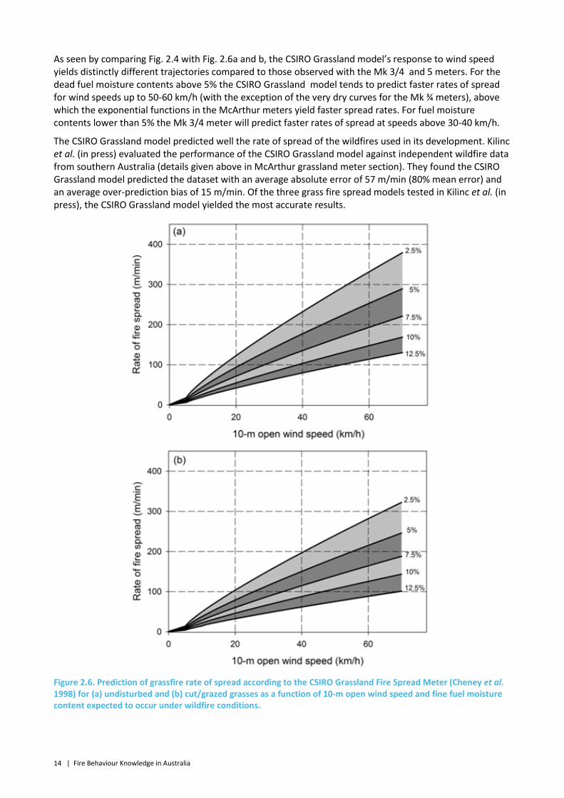
As seen by comparing Fig. 2.4 with Fig. 2.6a and b, the CSIRO Grassland model’s response to wind speed yields distinctly different trajectories compared to those observed with the Mk 3/4 and 5 meters. For the dead fuel moisture contents above 5% the CSIRO Grassland model tends to predict faster rates of spread for wind speeds up to 50-60 km/h (with the exception of the very dry curves for the Mk ¾ meters), above which the exponential functions in the McArthur meters yield faster spread rates. For fuel moisture contents lower than 5% the Mk 3/4 meter will predict faster rates of spread at speeds above 30-40 km/h.
The CSIRO Grassland model predicted well the rate of spread of the wildfires used in its development. Kilinc et al. (in press) evaluated the performance of the CSIRO Grassland model against independent wildfire data from southern Australia (details given above in McArthur grassland meter section). They found the CSIRO Grassland model predicted the dataset with an average absolute error of 57 m/min (80% mean error) and an average over-prediction bias of 15 m/min. Of the three grass fire spread models tested in Kilinc et al. (in press), the CSIRO Grassland model yielded the most accurate results.
Figure 2.6. Prediction of grassfire rate of spread according to the CSIRO Grassland Fire Spread Meter (Cheney et al. 1998) for (a) undisturbed and (b) cut/grazed grasses as a function of 10-m open wind speed and fine fuel moisture content expected to occur under wildfire conditions.
Fire Behaviour Knowledge in Australia | 15
2.2.2 HUMMOCK SPINIFEX GRASSLANDS
Griffin and Allan (1984)
Model description
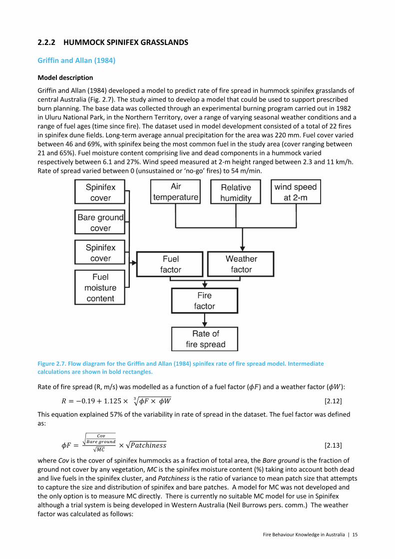
Griffin and Allan (1984) developed a model to predict rate of fire spread in hummock spinifex grasslands of central Australia (Fig. 2.7). The study aimed to develop a model that could be used to support prescribed burn planning. The base data was collected through an experimental burning program carried out in 1982 in Uluru National Park, in the Northern Territory, over a range of varying seasonal weather conditions and a range of fuel ages (time since fire). The dataset used in model development consisted of a total of 22 fires in spinifex dune fields. Long-term average annual precipitation for the area was 220 mm. Fuel cover varied between 46 and 69%, with spinifex being the most common fuel in the study area (cover ranging between 21 and 65%). Fuel moisture content comprising live and dead components in a hummock varied respectively between 6.1 and 27%. Wind speed measured at 2-m height ranged between 2.3 and 11 km/h. Rate of spread varied between 0 (unsustained or ‘no-go’ fires) to 54 m/min.
Figure 2.7. Flow diagram for the Griffin and Allan (1984) spinifex rate of fire spread model. Intermediate calculations are shown in bold rectangles.
Rate of fire spread (R, m/s) was modelled as a function of a fuel factor (𝜙𝐹) and a weather factor (𝜙𝑊):
𝑅 = −0.19 + 1.125 × �𝜙𝐹 × 𝜙𝑊3 [2.12]
This equation explained 57% of the variability in rate of spread in the dataset. The fuel factor was defined as:
𝜙𝐹 = � 𝐶𝑜𝑣𝐵𝑎𝑟𝑒 𝑔𝑟𝑜𝑢𝑛𝑑
√𝑀𝐶 × √𝑃𝑎𝑡𝑐ℎ𝑖𝑛𝑒𝑠𝑠 [2.13]
where Cov is the cover of spinifex hummocks as a fraction of total area, the Bare ground is the fraction of ground not cover by any vegetation, MC is the spinifex moisture content (%) taking into account both dead and live fuels in the spinifex cluster, and Patchiness is the ratio of variance to mean patch size that attempts to capture the size and distribution of spinifex and bare patches. A model for MC was not developed and the only option is to measure MC directly. There is currently no suitable MC model for use in Spinifex although a trial system is being developed in Western Australia (Neil Burrows pers. comm.) The weather factor was calculated as follows:

16 | Fire Behaviour Knowledge in Australia
𝜙𝑊 = �𝑇×𝑒𝑥𝑝(𝑈2)𝑅𝐻
[2.14]
where T is the air temperature (°C), U2 the wind speed measured at 2-m (m/s) and RH the air relative humidity (%).
Model behaviour and evaluation
The use of an exponential function for wind speed makes this variable the most influential one in the model. Figure 2.8 presents the sensitivity of Griffin and Allan (1984) model to wind speed and fuel moisture content. The model is relatively insensitive to changes in wind speed in the lower range of this variable and highly sensitive in the upper ranger, resulting in exceedingly high rates of spread if the model is used with high wind speeds. The model also shows a relatively small effect of fuel moisture content on the spread rate of the fire.
The adopted model form, without any coefficient directly linked to input variables, means that none of the variables, with the exception of wind speed, show a decisive effect on the rate of spread of the fire. It is uncertain if this is the result of the characteristics of the original dataset or due to the modelling options employed by its authors. Given the model form it is recommended that the model not be used outside of the bounds of the original dataset, i.e., it should only be used to predict fire behaviour under prescribed burning conditions.
Figure 2.8. Prediction of rate of fire spread in Spinifex according to the Griffin and Allan (1984) model as a function of 10-m open wind speed and fine fuel moistures content expected to occur under prescribed burning conditions. Flat ground, air temperature 31°C, relative humidity 10%, Cov 39%, Bare ground 42% and Patchiness 0.8 are assumed. A wind correction factor of 0.7 was used to convert 10-m open into 2-m wind speeds.
Burrows et al. (1991) evaluated the Griffin and Allan (1984) model against fire spread data (n = 58) collected in experimental prescribed fires in spinifex vegetation in the Gibson Desert Nature Reserve of Western Australia. Rate of spread in this dataset varied between 4.3 and 66.6 m/min, a range similar to the Griffin and Allan (1984) dataset. Burrows et al. (1991) found that the Griffin and Allan (1984) model to largely over predict his dataset. All of the experimental prescribed fires were over-predicted resulting in an average error of -43.4 m/min (217%).

Fire Behaviour Knowledge in Australia | 17
Burrows et al. (1991)
Model description
Burrows et al. (1991) conducted an experimental burning study in desert spinifex grasslands of Western Australia with the ultimate aim of developing an operational fire spread model for spinifex fuels (Fig. 2.9). The study area was the Gibson Desert (desert climate with average annual rainfall of 220 mm). The fuel complex can be described as predominantly hummock clumps of Plectrachne spp. and Triodia spp. with scattered low grasses and other shrub vegetation of various species.
Figure 2.9. Flow diagram for the Burrows et al. (1991) spinifex rate of fire spread model.
The fuel complex at four distinct sites was characterized for patchiness and spatial distribution, fuel load (varying between 0.3 and 13.5 t/ha), fuel height (varying between 0.18 and 0.28 m), compactness and fuel particle size. A total of 41 experimental fires with rates of spread varying between 0 (self extinguished fire) to 92 m/min and fireline intensities up to 14,630 kW/m. Relevant weather variables measured included 2-m wind speeds (range: 4 to 36 km/h), air temperature (range: 19 to 50°C) and relative humidity (range: 14 to 48%). Fuel moisture content, a composite of dead and live fuels, varied between 12 and 31%. A model for rate of spread was developed from stepwise multiple linear regression analysis:
𝑅 = 3.9 × 𝑈22 − 82.08 × 𝑀𝐶 + 5826.36 × (𝐶𝑜𝑣𝑅) + 43.5 × 𝑇 – 4935.29 [2.15]
where R is in m/h, U2 is wind speed measured at a 2-m height (km/h), MC constituting the compounded fuel moisture content (%) incorporating both dead and live components, CovR is the ratio between the spinifex cover (%) and the bare ground cover (%) and T the air temperature (°C) (Fig 2.9). Due to the scattered nature of the hummock fuels a 12-17 km/h threshold wind speed was deemed necessary for sustained head-fire spread. No back and flank fire propagation was observed in these fire experiments. No model for MC was presented.
Model behaviour and evaluation
Figure 2.10 presents the sensitivity of Burrows et al. (1991) rate of fire spread model to wind velocity and fuel moisture content (aggregate of live and dead fuels). The patchy fuel distribution that characterises spinifex fuel types (Gill et al. 1995) makes wind speed the main driver of fire propagation, and this is mathematically implied by the power law function of wind speed given in Eq. 2.15. Without the presence of wind to increase heat transfer between burning and unburned clumps, fire will fail to propagate (see Bradstock and Gill 1993). The effect of fuel moisture content on rate of fire spread is relatively small. The cover ratio (spinifex cover / bare ground cover) is the fuel characteristic describing the fuel complex state and has an approximate linear effect on the fire spread rate. An increase (or reduction) in spinifex cover by 25% will result in a homologous change in rate of spread. Although this fuel variable only considers two aspects of vegetation, in reality it also takes into account the effect of other fuel components such as ephemeral grasses that occur after periods of high rainfall on rate of spread. As pointed out by Burrows et al. (1991), the model represented by Eq. 2.15 is bounded by the intervals in the environmental variables described above.
18 | Fire Behaviour Knowledge in Australia
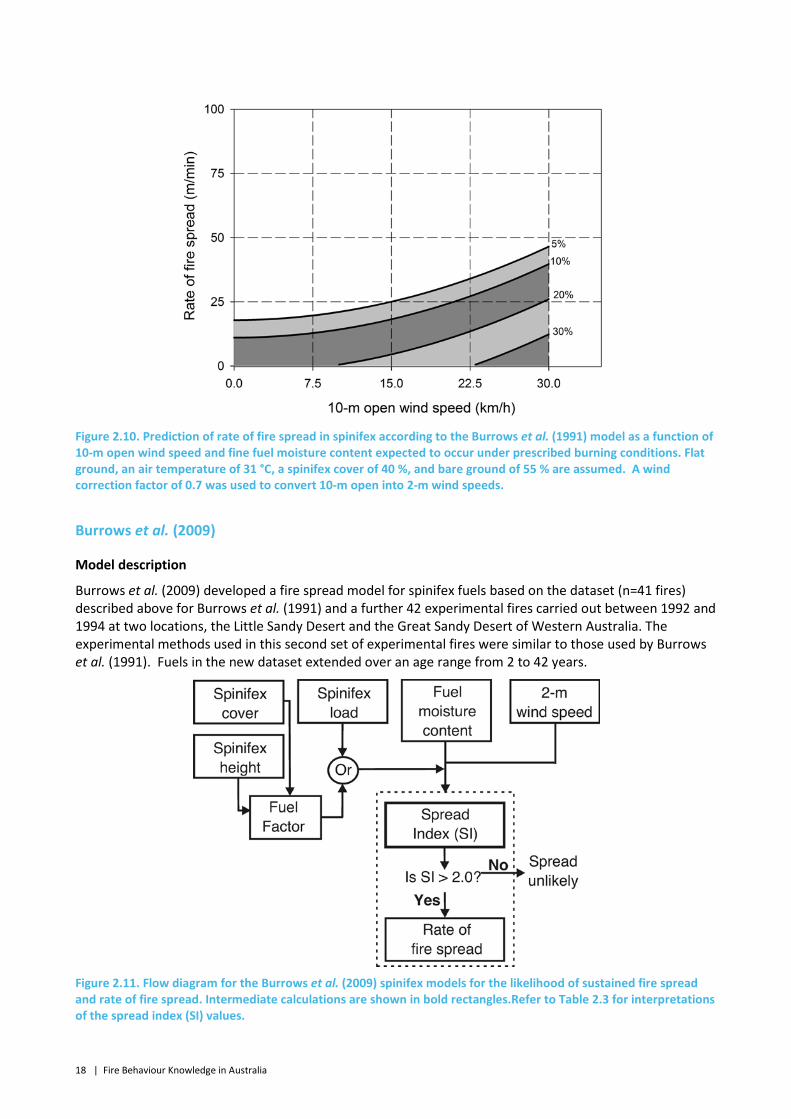
Figure 2.10. Prediction of rate of fire spread in spinifex according to the Burrows et al. (1991) model as a function of 10-m open wind speed and fine fuel moisture content expected to occur under prescribed burning conditions. Flat ground, an air temperature of 31 °C, a spinifex cover of 40 %, and bare ground of 55 % are assumed. A wind correction factor of 0.7 was used to convert 10-m open into 2-m wind speeds.
Burrows et al. (2009)
Model description
Burrows et al. (2009) developed a fire spread model for spinifex fuels based on the dataset (n=41 fires) described above for Burrows et al. (1991) and a further 42 experimental fires carried out between 1992 and 1994 at two locations, the Little Sandy Desert and the Great Sandy Desert of Western Australia. The experimental methods used in this second set of experimental fires were similar to those used by Burrows et al. (1991). Fuels in the new dataset extended over an age range from 2 to 42 years.
Figure 2.11. Flow diagram for the Burrows et al. (2009) spinifex models for the likelihood of sustained fire spread and rate of fire spread. Intermediate calculations are shown in bold rectangles.Refer to Table 2.3 for interpretations of the spread index (SI) values.

Fire Behaviour Knowledge in Australia | 19
Due to the discontinuous nature of fuels in these arid environments the application of a fire spread model requires a prior assessment of the likelihood of sustained fire spread (Gill et al. 1995). Using the combined datasets the authors aimed to develop models to (i) determine threshold conditions for sustained fire spread (‘go’ /‘no-go’) and (ii) predict the spread rate of a free burning fire (Fig. 2.11). The authors formulated two distinct model groups taking into account the fuel complex variables used to describe fuel structure. We will first describe the model group that uses fuel load as an input, followed by a description of the second model that uses hummock cover and height as fuel input variables.
The model for fire propagation starts with the calculation of a Fire Spread Index (SIFL):
𝑆𝐼𝐹𝐿 = 0.57 × 𝑈2 + 0.96 × 𝑤 − 0.42 × 𝑀𝐶 − 7.42 [2.16]
where U2 is the average wind speed (km/h) measured over a 5-min period at a height of 2-m, w is spinifex and other fine fuel load (t/ha) and MC is the compounded fuel moisture content (%) incorporating both dead and live fuel components. As with the other spinifex studies no model for estimating MC was developed and measured values or best estimates must be used.
The SIFL describes the likelihood of a fire to spread. If SIFL < 0, then it is unlikely that sustained fire spread will occur. For SIFL values > 0, the more likely that a free-spreading fire spread will occur. Burrows et al. (2009) provide a Spread Index interpretation table (Table 2.3).
Table 2.3. Interpretation of Burrows et al. (2009) Fire Spread Index (SIFL and SIFF) in terms of likelihood of sustained fire spread and accordingly rate of fire spread in spinifex grasslands.
SI LIKELIHOOD OF FIRE SPREAD POTENTIAL ROS (M/H) SI ≤ -2 Fire unlikely to spread 0 -2 < SI ≤0 Fire may spread < 500 0 < SI ≤ 2 Fire should spread 500 – 900 2 < SI ≤ 4 Fire will spread 900 – 1800 4 < SI ≤ 6 Fire will spread 1800 – 2700 6 < SI ≤ 10 Fire will spread 2700 – 4500 SI ≥10 Fire will spread >4500
If the Fire Spread Index indicates that a fire is likely to spread then the fire rate of forward spread (ROSFL, m/h) is calculated as:
𝑅𝑂𝑆𝐹𝐿 = 1581 + 154.9 × 𝑈2 + 140.6 × 𝑤 − 228.0 × 𝑀𝐶 [2.17]
The alternative Fire Spread Index model that uses fuel cover and height instead of fuel load is:
𝑆𝐼𝐹𝐹 = 0.37 × 𝑈2 + 0.78 × 𝐹𝐹 − 0.31 × 𝑀𝐶 − 5.23 [2.18]
where FF is the fuel factor:
𝐹𝐹 = 0.25 × 𝐶𝑜𝑣 + 0.04 × 𝐹𝐻 − 0.32 [2.19]
where Cov represents the spinifex cover (%) and FH is the mean hummock height (cm). The interpretation of the Fire Spread Index in Table 2.3 are also applicable to the SIFF. The rate of fire spread calculated using the the fuel factor (ROSFL, m/h) is:
𝑅𝑂𝑆𝐹𝐹 = 1969 + 142.8 × 𝑈2 + 120.1 × 𝐹𝐹 − 229.1 × 𝑀𝐶 [2.20]
Model behaviour and evaluation
The model form adopted by Burrows et al. (2009) results in significantly different results compared to the Griffin and Allan (1984) and the original Burrows et al. (1991) models. Burrows et al. (2009) explicitly considered a function to determine fire spread sustainability after which the rate of fire spread is calculated. Wind speed, fuel moisture content and fuel load (a surrogate of spinifex cover and age) all have a significant effect on the likelihood of fire spread (Fig 2.12).
20 | Fire Behaviour Knowledge in Australia
The wind function imposes a linear effect on rate of spread that is lower than that found in the other spinifex fire spread rate models. Conversely, the effect of fuel moisture content is observed to have a stronger influence than in previous models. The sensitivity of rate of spread to fuel load is lower than found for the two variables described above. A doubling in fuel load will increase rate of spread by about 13%. We are presently unaware of any published evaluation on the performance of the Burrows et al. (2009) models against independent datasets.
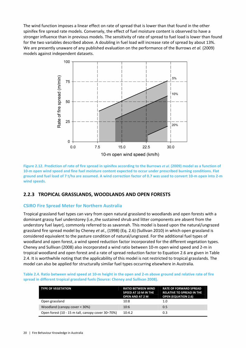
Figure 2.12. Prediction of rate of fire spread in spinifex according to the Burrows et al. (2009) model as a function of 10-m open wind speed and fine fuel moisture content expected to occur under prescribed burning conditions. Flat ground and fuel load of 7 t/ha are assumed. A wind correction factor of 0.7 was used to convert 10-m open into 2-m wind speeds.
2.2.3 TROPICAL GRASSLANDS, WOODLANDS AND OPEN FORESTS
CSIRO Fire Spread Meter for Northern Australia
Tropical grassland fuel types can vary from open natural grassland to woodlands and open forests with a dominant grassy fuel understorey (i.e.,the sustained shrub and litter components are absent from the understory fuel layer), commonly referred to as savannah. This model is based upon the natural/ungrazed grassland fire spread model by Cheney et al., (1998) (Eq. 2.6) (Sullivan 2010) in which open grassland is considered equivalent to the pasture condition of natural/ungrazed. For the additional fuel types of woodland and open forest, a wind speed reduction factor incorporated for the different vegetation types. Cheney and Sullivan (2008) also incorporated a wind ratio between 10-m open wind speed and 2-m in tropical woodland and open forest and a rate of spread reduction factor to Equation 2.6 are given in Table 2.4. It is worthwhile noting that the applicability of this model is not restricted to tropical grasslands. The model can also be applied for structurally similar fuel types occurring elsewhere in Australia.
Table 2.4. Ratio between wind speed at 10-m height in the open and 2-m above ground and relative rate of fire spread in different tropical grassland fuels (Source: Cheney and Sullivan 2008).
TYPE OF VEGETATION RATIO BETWEEN WIND SPEED AT 10 M IN THE OPEN AND AT 2 M
RATE OF FORWARD SPREAD RELATIVE TO SPREAD IN THE OPEN (EQUATION 2.6)
Open grassland 10:8 1.0 Woodland (canopy cover < 30%) 10:6 0.5 Open forest (10 - 15 m tall, canopy cover 30–70%) 10:4.2 0.3

Fire Behaviour Knowledge in Australia | 21
2.3 Shrublands
Shrubland vegetation in Australia can be found in a range of environments, ranging from coastal dunes to mountainous uplands, and are commonly associated with shallow or sandy soils of low nutrient status (Hollis et al. in review). Prominent features of heath/shrubland communities are their floristic diversity and propensity for recurrent fire. In Australia models have been developed to predict the spread of fire in Tasmanian buttongrass moorlands, temperate heathlands and semi-arid mallee-heath.
2.3.1 BUTTONGRASS MOORLANDS
Marsden-Smedley and Catchpole (1995b)
Model description
Marsden-Smedley and Catchpole (1995b) described the fire behaviour modelling component of a study aimed at developing a comprehensive fire danger and fire behaviour prediction system for Tasmanian buttongrass moorlands (Fig. 2.13). Buttongrass moorlands, a significant Tasmania vegetation type, are defined as treeless communities dominated by sedges and low heaths with a significant contribution of buttongrass Gymnoschoenus sphaerocephalus (Marsden-Smedley and Catchpole 1995a).
Figure 2.13. Flow diagram for Marsden-Smedley and Catchpole (1995b) model for predicting the rate of fire spread in buttongrass moorlands.
Key fuel complex components are the openness of the fuels to wind flow and the substantial quantity of suspended dead fuels within the hummocks. These features make the fuel complex susceptible to sustain fire propagation even when soil and litter fuel moisture content levels are quite high.
Fire behaviour data was measured in a total of 64 fires, comprising experimental fires (n=44), operational prescribed fires (n=11) and wildfires (n=5). Fuel age in the experimental fires varied between 4 and 25 years. Fire environmental and behaviour characteristics of the dataset used in model development varied over a wide range. Dead fuel moisture content, wind speed and rate of spread varied between 8.2 and 68%, 0.7 and 36 km/h, and 0.6 and 55 m/min, respectively.
Non-linear regression analysis was used to model the headfire rate of spread (R, m/min):
𝑅 = 0.678 × 𝑈21.312 × 𝑒𝑥𝑝(−0.0243 × 𝑀𝐶) × �1 − 𝑒𝑥𝑝(−0.116 × 𝐴𝐺𝐸)� [2.21]
with U2 being the wind speed (km/h) measured at 2-m height, MC is the dead fuel moisture content (%) and AGE is time since the last fire in years, a surrogate of other fuel characteristics such as fuel load and fraction of dead fuel (Fig 2.13). Marsden-Smedley and Catchpole (2001) tested several MC models of which the best was:
𝑀𝐶 = 𝑒𝑥𝑝(1.660 + 0.0214 × 𝑅𝐻 − 0.0292 × 𝑇𝑑𝑒𝑤) [2.22]
22 | Fire Behaviour Knowledge in Australia
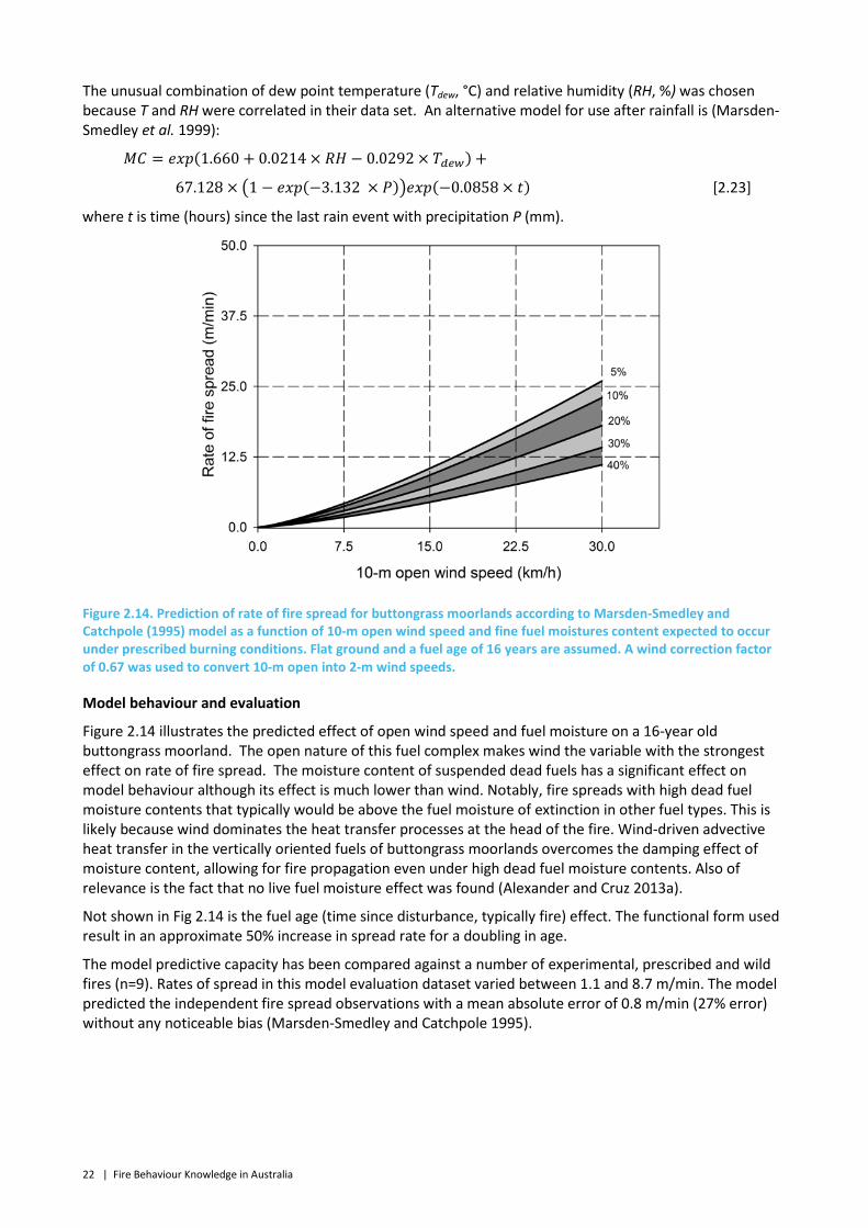
The unusual combination of dew point temperature (Tdew, °C) and relative humidity (RH, %) was chosen because T and RH were correlated in their data set. An alternative model for use after rainfall is (Marsden-Smedley et al. 1999):
𝑀𝐶 = 𝑒𝑥𝑝(1.660 + 0.0214 × 𝑅𝐻 − 0.0292 × 𝑇𝑑𝑒𝑤) +
67.128 × �1 − 𝑒𝑥𝑝(−3.132 × 𝑃)�𝑒𝑥𝑝(−0.0858 × 𝑡) [2.23]
where t is time (hours) since the last rain event with precipitation P (mm).
Figure 2.14. Prediction of rate of fire spread for buttongrass moorlands according to Marsden-Smedley and Catchpole (1995) model as a function of 10-m open wind speed and fine fuel moistures content expected to occur under prescribed burning conditions. Flat ground and a fuel age of 16 years are assumed. A wind correction factor of 0.67 was used to convert 10-m open into 2-m wind speeds.
Model behaviour and evaluation
Figure 2.14 illustrates the predicted effect of open wind speed and fuel moisture on a 16-year old buttongrass moorland. The open nature of this fuel complex makes wind the variable with the strongest effect on rate of fire spread. The moisture content of suspended dead fuels has a significant effect on model behaviour although its effect is much lower than wind. Notably, fire spreads with high dead fuel moisture contents that typically would be above the fuel moisture of extinction in other fuel types. This is likely because wind dominates the heat transfer processes at the head of the fire. Wind-driven advective heat transfer in the vertically oriented fuels of buttongrass moorlands overcomes the damping effect of moisture content, allowing for fire propagation even under high dead fuel moisture contents. Also of relevance is the fact that no live fuel moisture effect was found (Alexander and Cruz 2013a).
Not shown in Fig 2.14 is the fuel age (time since disturbance, typically fire) effect. The functional form used result in an approximate 50% increase in spread rate for a doubling in age.
The model predictive capacity has been compared against a number of experimental, prescribed and wild fires (n=9). Rates of spread in this model evaluation dataset varied between 1.1 and 8.7 m/min. The model predicted the independent fire spread observations with a mean absolute error of 0.8 m/min (27% error) without any noticeable bias (Marsden-Smedley and Catchpole 1995).
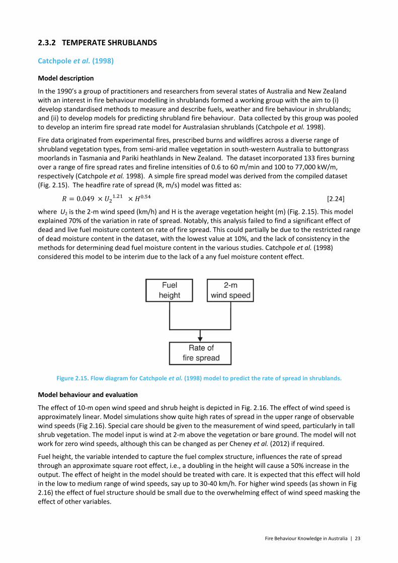
Fire Behaviour Knowledge in Australia | 23
2.3.2 TEMPERATE SHRUBLANDS
Catchpole et al. (1998)
Model description
In the 1990’s a group of practitioners and researchers from several states of Australia and New Zealand with an interest in fire behaviour modelling in shrublands formed a working group with the aim to (i) develop standardised methods to measure and describe fuels, weather and fire behaviour in shrublands; and (ii) to develop models for predicting shrubland fire behaviour. Data collected by this group was pooled to develop an interim fire spread rate model for Australasian shrublands (Catchpole et al. 1998).
Fire data originated from experimental fires, prescribed burns and wildfires across a diverse range of shrubland vegetation types, from semi-arid mallee vegetation in south-western Australia to buttongrass moorlands in Tasmania and Pariki heathlands in New Zealand. The dataset incorporated 133 fires burning over a range of fire spread rates and fireline intensities of 0.6 to 60 m/min and 100 to 77,000 kW/m, respectively (Catchpole et al. 1998). A simple fire spread model was derived from the compiled dataset (Fig. 2.15). The headfire rate of spread (R, m/s) model was fitted as:
𝑅 = 0.049 × 𝑈21.21 × 𝐻0.54 [2.24]
where U2 is the 2-m wind speed (km/h) and H is the average vegetation height (m) (Fig. 2.15). This model explained 70% of the variation in rate of spread. Notably, this analysis failed to find a significant effect of dead and live fuel moisture content on rate of fire spread. This could partially be due to the restricted range of dead moisture content in the dataset, with the lowest value at 10%, and the lack of consistency in the methods for determining dead fuel moisture content in the various studies. Catchpole et al. (1998) considered this model to be interim due to the lack of a any fuel moisture content effect.
Figure 2.15. Flow diagram for Catchpole et al. (1998) model to predict the rate of spread in shrublands.
Model behaviour and evaluation
The effect of 10-m open wind speed and shrub height is depicted in Fig. 2.16. The effect of wind speed is approximately linear. Model simulations show quite high rates of spread in the upper range of observable wind speeds (Fig 2.16). Special care should be given to the measurement of wind speed, particularly in tall shrub vegetation. The model input is wind at 2-m above the vegetation or bare ground. The model will not work for zero wind speeds, although this can be changed as per Cheney et al. (2012) if required.
Fuel height, the variable intended to capture the fuel complex structure, influences the rate of spread through an approximate square root effect, i.e., a doubling in the height will cause a 50% increase in the output. The effect of height in the model should be treated with care. It is expected that this effect will hold in the low to medium range of wind speeds, say up to 30-40 km/h. For higher wind speeds (as shown in Fig 2.16) the effect of fuel structure should be small due to the overwhelming effect of wind speed masking the effect of other variables.
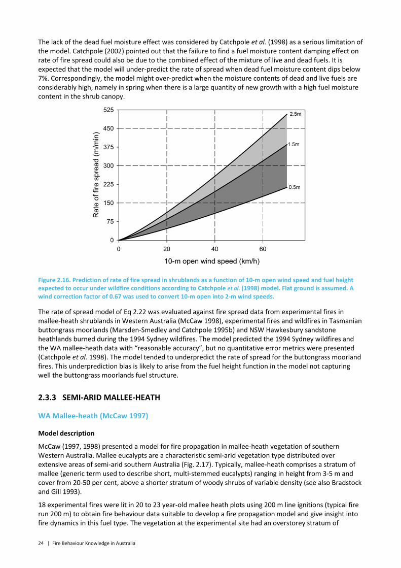
24 | Fire Behaviour Knowledge in Australia
The lack of the dead fuel moisture effect was considered by Catchpole et al. (1998) as a serious limitation of the model. Catchpole (2002) pointed out that the failure to find a fuel moisture content damping effect on rate of fire spread could also be due to the combined effect of the mixture of live and dead fuels. It is expected that the model will under-predict the rate of spread when dead fuel moisture content dips below 7%. Correspondingly, the model might over-predict when the moisture contents of dead and live fuels are considerably high, namely in spring when there is a large quantity of new growth with a high fuel moisture content in the shrub canopy.
Figure 2.16. Prediction of rate of fire spread in shrublands as a function of 10-m open wind speed and fuel height expected to occur under wildfire conditions according to Catchpole et al. (1998) model. Flat ground is assumed. A wind correction factor of 0.67 was used to convert 10-m open into 2-m wind speeds.
The rate of spread model of Eq 2.22 was evaluated against fire spread data from experimental fires in mallee-heath shrublands in Western Australia (McCaw 1998), experimental fires and wildfires in Tasmanian buttongrass moorlands (Marsden-Smedley and Catchpole 1995b) and NSW Hawkesbury sandstone heathlands burned during the 1994 Sydney wildfires. The model predicted the 1994 Sydney wildfires and the WA mallee-heath data with “reasonable accuracy”, but no quantitative error metrics were presented (Catchpole et al. 1998). The model tended to underpredict the rate of spread for the buttongrass moorland fires. This underprediction bias is likely to arise from the fuel height function in the model not capturing well the buttongrass moorlands fuel structure.
2.3.3 SEMI-ARID MALLEE-HEATH
WA Mallee-heath (McCaw 1997)
Model description
McCaw (1997, 1998) presented a model for fire propagation in mallee-heath vegetation of southern Western Australia. Mallee eucalypts are a characteristic semi-arid vegetation type distributed over extensive areas of semi-arid southern Australia (Fig. 2.17). Typically, mallee-heath comprises a stratum of mallee (generic term used to describe short, multi-stemmed eucalypts) ranging in height from 3-5 m and cover from 20-50 per cent, above a shorter stratum of woody shrubs of variable density (see also Bradstock and Gill 1993).
18 experimental fires were lit in 20 to 23 year-old mallee heath plots using 200 m line ignitions (typical fire run 200 m) to obtain fire behaviour data suitable to develop a fire propagation model and give insight into fire dynamics in this fuel type. The vegetation at the experimental site had an overstorey stratum of

Fire Behaviour Knowledge in Australia | 25
Eucalyptus pleurocarpa and Eucalyptus pachyloma, an intermediate stratum up to 2.5 m tall of Xanthorrhoea platyphylla, Hakea crassifolia, Banksia falcata and Banksia sessilis, and a species-rich layer of dwarf shrubs up to 1 m in height.
Figure 2.17. Flow diagram for McCaw (1997) mallee-heath rate of fire spread model.
Experiments spanned a broad range of fire weather conditions with the most intense fires having forward rates of spread up to 40 m/min and fireline intensities up to 14,000 kW/m. Of the 18 experimental fires, nine fires failed to spread (i.e., “no-go” fires). Although the size of the dataset did not allow for factors determining fire sustainability to be modelled, the moisture content of the shallow litter layer beneath the low shrubs was found to have a controlling influence on the likelihood of fire spread. Fires spread freely when the moisture content of the shallow litter was below 8 %, regardless of the prevailing wind speed.
The forward rate of spread (R, m/sec) was modelled through non-linear regression analysis, with the best fit given by:
𝑅 = 0.292 × 𝑈21.05 × 𝑒𝑥𝑝(−0.11 ×𝑀𝐶𝑙𝑑) [2.25]
where U2 is the wind speed (m/sec) measured in the open at a 2-m height, and MCld is the moisture content of the deep litter beneath mallee clumps (Fig. 2.17). McCaw (1997) found the Nelson (1991) fuel moisture model was the best fitting of several tested, and a guide based on that model using time of day and predetermined values of air temperature and relative humidity for two typical weather patterns, was used operationally until 2008 in Western Australia. Since then the fuel moisture model from the Dry Eucalypt Forest model (Gould et al. 2007b) derived from the process-based model of Matthews (2006) has been used.
Figure 2.18. Prediction of rate of fire spread in mallee-heath shrublands as a function of 10-m open wind speed and fine fuel moisture content expected to occur under wildfire conditions as predicted by the McCaw (1997) model. Flat ground is assumed. A wind correction factor of 0.67 was used to convert 10-m open into 2-m wind speeds.
26 | Fire Behaviour Knowledge in Australia
The model represented by eq. 2.25 accounted for 84 per cent of variation in the spread rate of the experimental fires. Experimental fires were conducted in a relatively uniform stands of mallee heath which precluded the investigation of the influence of fuel structure on rate of fire spread. As in other shrubland fire spread models, no significant live fuel moisture effect was found (see also Alexander and Cruz 2013a).
Model behaviour and evaluation
The general effect of open wind speed and fuel moisture on the McCaw (1997) rate of spread model for mallee-heath shrublands is given in Fig 2.18. The functional form and parameterization of the wind and fuel moisture effect in this model is similar to that found in studies by Cheney et al. (1998) for grasslands and Marsden-Smedley and Catchpole (1995b) for buttongrass moorlands. Wind speed has an almost linear effect on rate of spread. Fuel moisture content effect follows an exponential decay function. It was also found that sustained fire propagation required fuel moistures to drop below 8%. This threshold can be expected to change after high rainfall period when the increased growth in ephemeral grass could lead to reduced fuel discontinuity. After such events the fuel moisture threshold might increase, although it is not expected that the rate of fire spread sensitivity to environemtal drivers would change.
The predictions in rate of spread from the model matched well with observations from a limited number of prescribed fires and wild-fires involving spread rates up to 61 m/min.
South Australia semi-arid mallee heath (Cruz et al. 2010)
Model description
Cruz et al. (2010) conducted a experimental fire behaviour study between 2006 and 2008 at the Ngarkat Conservation Park, South Australia. Annual rainfall in the area averages 473 mm. Vegetation was characterised as open woodland with Eucalyptus calycogona, Eucalyptus diversifolia, Eucalyptus incrassata and Eucalyptus leptophylla as dominant overstorey species. The vegetation had three age classes as a result of wildfires in 1958 (48 to 50 year old fuels), 1986 (20 to 22 year old fuels) and 1999 (7 to 9 year old fuels). Plot sizes varied between approximately 70 m × 70 m for fire sustainability experiments and 750 m × 750 m for the larger fire behaviour experiments.
A total of 67 experimental fires were conducted in plots ranging from 1 to 6 ha in size under a wide range of burning conditions. A number of plots were burned within Very High Forest Fire Danger Rating (35< FFDI<50) conditions to capture data representative of typical wildfire burning environment. Dead fuel moisture contents and 10-m open wind speed varied respectively between 2 – 20% and 2 – 24 km/h. Fire behaviour ranged from self-extinguishing fires to sustained active crown fire propagation. Rates of spread in sustained fires ranged from 3 to 58 m/min.
In developing a system to predict fire behaviour in mallee-heath fuel complexes Cruz et al. (2010) recognized that model users in distinct situations would need to conduct fire behaviour potential assessments with different types of available input variables. Two typical situations were identified where models could be used. Fire behaviour predictions conducted in an office environment are commonly based on weather station data or forecasted weather, namely using wind speeds measured/predicted at 10-m in the open. In field settings the model usage would be relying on local wind measurements made at eye-level (~ 2-m high) within the mallee-heath stand. To minimize errors introduced wind speed conversion the authors developed two groups of models, one relying on 10-m open wind speed based on wind speeds measured at eye-level. To extend the applicability of the mallee-heath models in supporting fire management decision-making, alternative models were developed where distinct fuel input variables were used. Herein we will solely describe the models converted into a field based prescribed burning guide (Cruz 2010).
The models are integrated into a fire behaviour prediction system (Fig. 2.19) most applicable to prescribed fire burning conditions in mallee-heath fuels, and extending into Very High to Extreme Fire Danger Rating classes. The system integrates a series of models aimed at predicting various fire characteristics required by fire managers to plan and conduct prescribed burns.

Fire Behaviour Knowledge in Australia | 27
Figure 2.19. Flow diagram for Cruz et al. (2010) model to predict the rate of spread in mallee-heath srublands.
The system comprises the following sub models:
The probability of successful fire spread was modelled using logistic regression analysis:
Ps(y=1)= 11+exp(2.926+2.132 ×𝑈2+2.32×MCsus+5.31× 𝑃𝐶𝑆el)
[2.26]
where Ps(y = 1) is the probability that a self-sustained surface fire will occur, U2 the 2-m wind speed (km/h), MCsus is the moisture content (%) of dead suspended fuels, and PCSel is the elevated fuel layer Percent Cover Score. The cut-off value between non-spreading and spreading fires is 0.5 (i.e. fires are expected to spread if the probability is higher than 50%). Overall, this model predicted correctly 93% of the modelling dataset.

28 | Fire Behaviour Knowledge in Australia
Nomograms for calculating mallee and heath MC from calendar date, cloud cover, T and RH are included in Cruz et al. (2010). These may be approximated for mallee as:
𝑀𝐶 = 4.79 + 0.173 × 𝑅𝐻 − 0.1 × (𝑇 − 25) − ∆ 0.027 × 𝑅𝐻 [2.27a]
where Δ = 1 for sunny days from 12:00-17:00 from October to March (i.e. high solar radiation) and 0 otherwise, and for heath:
𝑀𝐶 = 4.37 + 0.161 × 𝑅𝐻 − 0.1 × (𝑇 − 25) − ∆ 0.027 × 𝑅𝐻 [2.27b]
The probability of crown fire occurrence (Pc) was also modelled through logistic regression analysis as a function of 10-m open wind speed:
𝑃𝑐(𝑦 = 1) = 11+𝑒𝑥𝑝(−13.979+0.878× 𝑈10)
[2.28]
As before, the cut-off value between surface and crown was set at 0.5 (i.e. crown fires are expected to occur if the probability is higher than 50%). Overall, this model predicted correctly 77% of the modelling dataset.
Models for surface rate of spread were developed separately for pure heath and mallee-heath. For the mallee-heath fuel type separate surface and crown fire phase models were developed. Model parameterization relied on non-linear regression analysis. The surface fire rate of spread model for heath fuels was:
𝑅𝐻𝑒𝑎𝑡ℎ = 2.455 × 𝑈21.2 × 𝑒𝑥𝑝(−0.11 × 𝑀𝐶𝑠𝑢𝑠) × 𝐹𝐻𝑆𝑒𝑙0.90 [2.29]
where FHSel is the elevated fuel layer Fuel Hazard Score. This equation explained 82% of the variability in the dataset and predicted the original dataset with a mean absolute error of 51%.
The surface fire rate of spread model for mallee fuels was:
𝑅𝑀𝑎𝑙𝑙𝑒𝑒 = 2.053 × 𝑈21.1 × 𝑒𝑥𝑝(−0.11 × 𝑀𝐶𝑠𝑢𝑠) × 𝐹𝐻𝑆𝑒𝑙1.28 × 𝐻𝑂−0.72 [2.30]
where FHSel is the elevated fuel layer Fuel Hazard Score and HO is the height of the overstorey mallee stand. This equation explained 80% of the variability in the dataset and predicted the original dataset with a mean absolute error of 35%.
The best model to explain the spread rate of crown fires in mallee stands was:
𝑅𝐶 = 2.24 × 𝑈101.2 × 𝑒𝑥𝑝(−0.11 × 𝑀𝐶𝑠𝑢𝑠) [2.31]
This equation explained 80% of the variability in the dataset and predicted the original dataset with a mean absolute error of 35%.
Model behaviour and evaluation
Fig. 2.20 depicts the effect of wind speed and litter fuel moisture content on the type of fire and associated rate of spread for mallee heath stands. Both these variables are shown to have a pronounced effect on the likelihood of fire propagation. At fuel moisture contents of 5% or less, wind speed is not a necessary factor to maintain sustained fire propagation and active back and flank fire propagation will occur. For fuel moisture contents of 6% or higher wind speed is a necessary factor to induce fire propagation. It is worth noting that in these fuel moisture conditions and nil wind the fire might still propagate marginally within the litter of mallee clumps.

Fire Behaviour Knowledge in Australia | 29
Figure 2.20. Rate of fire spread in South Australian (a) heath and (b) mallee-heath shrublands as a function of 10-m open wind speed and fine fuel moistures content expected to occur under wildfire conditions as predicted by Cruz et al. (2010) model.
Semi-arid mallee heath (Cruz et al. 2013)
Model description
Cruz et al. (2013) merged the datasets of McCaw (1997) and Cruz et al. (2010) to develop a system of models for semi-arid mallee-heath fuel types to predict the likelihood of fire propagation (go/no-go), type of fire ( i.e., surface or crown), forward rate of fire spread, and flame height.
The overall dataset comprised 61 experimental fires conducted under the following range of fire weather conditions: 10-m open wind speed varied between 5 and 28 km/h; air temperature varied between 16 and 39°C; and relative humidity ranged from 7 to 80%. The total fuel load, comprised of litter, understorey shrubs and overstorey canopy fine fuels (leaves and live twigs with diameter <3 mm), varied between 3.8

30 | Fire Behaviour Knowledge in Australia
t/ha (in a 7-year old stand) and 14.8 t/ha (in a 21-year old stand). Thirty of the 61 fires failed to propagate following ignition and were classified as no-go fires. The average rate of fire spread and fireline intensity for the sustained fires varied between 4 and 55 m/min and 735 and 17,200 kW/m, respectively. Flame height varied between 1 and 8 m, with an average of 3.8 m.
The model system to predict the full range of fire behaviour in mallee-heath shrubland comprises linkages between five models (Fig. 2.21): (i) a model for fire spread sustainability (Eq. 2.32); if the environment conditions suggest that a fire will propagate then (ii) a model is used to determine the type of fire, i.e., surface or crown fire (Eq. 2.24); based on this result the rate of fire spread is determined for a surface (Eq. 2.35) or a crown fire (Eq. 2.36).
Figure 2.21. Flow diagram for the Cruz et al. (2013) model system to predict surface and crown fire rates of spread in mallee-heath shrublands.
Two groups of models were developed, one that required wind measured at 10-m in the open and the other where wind speed is measured at approximately 2-m height within a mallee-heath stand. We report here the models based on the 10-m open wind speed. The probability of successful fire spread was modelled using logistic regression analysis:

Fire Behaviour Knowledge in Australia | 31
𝑃𝑠(𝑦 = 1) = 11+𝑒𝑥𝑝�−(0.207 ×𝑈10−1.872 ×𝑀𝐶𝑙−30.442 ×𝐶𝑜𝑣𝑂)�
[2.32]
where Ps(y = 1) is the probability that a self-sustained surface fire will occur, U10 being the 10-m open wind speed (km/h), MCl is the moisture content (%) of the dead litter fuels, and CovO the overstorey mallee cover (%). The cut-off value between non-spreading and spreading fires was judged to be 0.5 (i.e. fires are expected to spread if the probability is higher than 50%). This model predicted correctly 94% of the modelling dataset.
Mallee and heath MC can be calculated from calendar date, cloud cover, T and RH:
𝑀𝐶𝑚𝑎𝑙𝑙𝑒𝑒 = 4.74 + 0.108 × 𝑅𝐻 − 0.1 × (𝑇 − 25) − ∆ × (1.68 + 0.028 × 𝑅𝐻) [2.33a]
𝑀𝐶ℎ𝑒𝑎𝑡ℎ = 4.20 + 0.129 × 𝑅𝐻 − 0.1 × (𝑇 − 25) − ∆ × (1.63 + 0.036 × 𝑅𝐻) [2.33b]
where Δ = 1 for sunny days from 12:00-17:00 from October to March (i.e. high solar radiation) and 0 otherwise
The probability of crown fire to occurrence was modelled through logistic regression analysis:
𝑃𝑐(𝑦 = 1) = 11+𝑒𝑥𝑝�−(1.4054× 𝑈10−3.4217 ×𝑀𝐶)�
[2.34]
where Pc(y = 1) is the probability that a crown fire will occur, with a cut-off value separating surface fires from crown fires at a value of 0.5. This model predicted correctly 78% of the modelling dataset.
Models for surface fire rate of spread and crown fire rate of spread were fitted using both log-linear and non-linear regression analysis. The surface fire rate of spread (RS, m/min) model was:
𝑅𝑆 = 3.337 × 𝑈101.0 × 𝑒𝑥𝑝(−0.1284 × 𝑀𝐶) × 𝐻𝑂−0.7073 [2.35]
where HO is the mallee overstorey height (m), an age dependent stand characteristic that in the model is a surrogate for other fuel characteristics. This equation explained 74% of the variability in the dataset.
The best model to explain the spread rate of crown fires (RC, m/min) was:
𝑅𝐶 = 9.5751 × 𝑈101.0 × 𝑒𝑥𝑝(−0.1751 × 𝑀𝐶) × 𝐶𝑜𝑣𝑂0.3589 [2.36]
The use of the model system requires first, an estimation of the likelihood of fire spread, Ps. If Ps <0.5, then it is assumed that a line ignition will be self extinguishing. If Ps >0.5, then the fire is assumed to result in sustained fire spread. For spreading fires the probability of crown fire propagation is then determined. If Pc <0.01, the fire is assumed to be spreading but largely controlled by the surface phase and surface fire behaviour characteristics are estimated. If Pc >0.99, crown fire propagation is assumed and the crown fire rate of spread model is applied. Recognizing the large uncertainty in predicted rate of fire spread around the 0.5 likelihood, where small errors in the input can lead to a substantial output errors, a weighted approach is used when 0.01< Pc <0.99. Within this Pc range a simple ensemble method is used with the final rate of fire spread (R) given by a weighted average of the surface (RS) and crown (RC) fire spread models outputs. The weighted factor is the probability or likelihood of crown fire propagation, PC:
[2.37]
Model behaviour and evaluation
Fig. 2.22 depicts the effect of wind speed and litter fuel moisture content on the type of fire and associated rate of spread. Both these variables are shown to have a pronounced effect on the likelihood of fire propagation. At fuel moisture contents of 5% or less, wind speed is not a necessary factor in maintaining sustained fire propagation and active back and flank fire propagation will occur. For fuel moisture contents of 6% or higher wind speed is a necessary factor to induce fire propagation. It is worth noting that in these
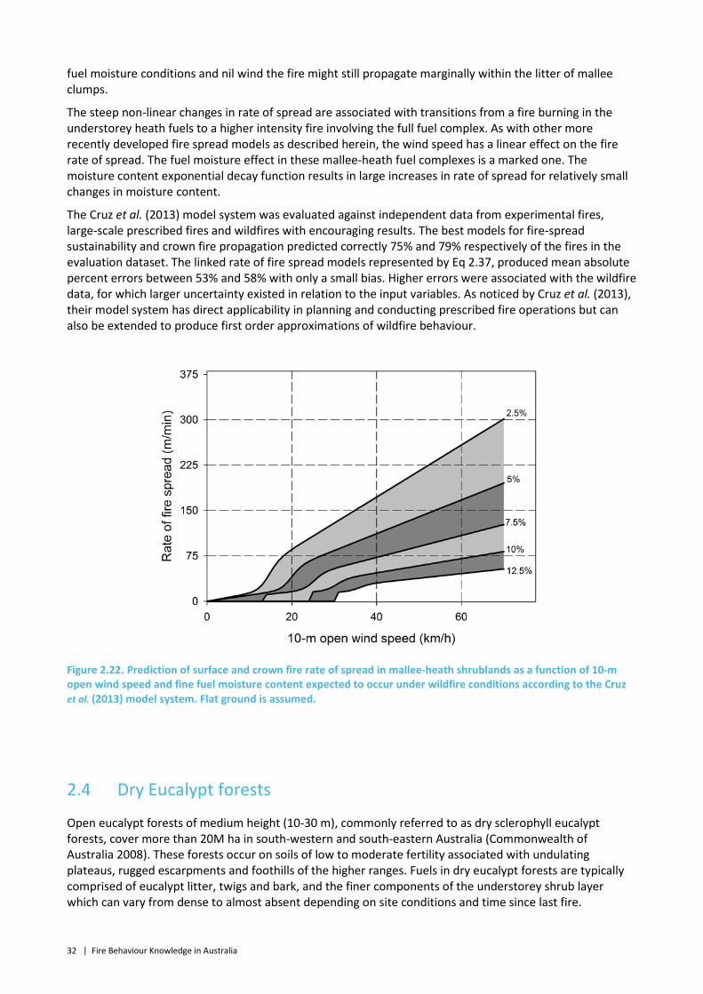
32 | Fire Behaviour Knowledge in Australia
fuel moisture conditions and nil wind the fire might still propagate marginally within the litter of mallee clumps.
The steep non-linear changes in rate of spread are associated with transitions from a fire burning in the understorey heath fuels to a higher intensity fire involving the full fuel complex. As with other more recently developed fire spread models as described herein, the wind speed has a linear effect on the fire rate of spread. The fuel moisture effect in these mallee-heath fuel complexes is a marked one. The moisture content exponential decay function results in large increases in rate of spread for relatively small changes in moisture content.
The Cruz et al. (2013) model system was evaluated against independent data from experimental fires, large-scale prescribed fires and wildfires with encouraging results. The best models for fire-spread sustainability and crown fire propagation predicted correctly 75% and 79% respectively of the fires in the evaluation dataset. The linked rate of fire spread models represented by Eq 2.37, produced mean absolute percent errors between 53% and 58% with only a small bias. Higher errors were associated with the wildfire data, for which larger uncertainty existed in relation to the input variables. As noticed by Cruz et al. (2013), their model system has direct applicability in planning and conducting prescribed fire operations but can also be extended to produce first order approximations of wildfire behaviour.
Figure 2.22. Prediction of surface and crown fire rate of spread in mallee-heath shrublands as a function of 10-m open wind speed and fine fuel moisture content expected to occur under wildfire conditions according to the Cruz et al. (2013) model system. Flat ground is assumed.
2.4 Dry Eucalypt forests
Open eucalypt forests of medium height (10-30 m), commonly referred to as dry sclerophyll eucalypt forests, cover more than 20M ha in south-western and south-eastern Australia (Commonwealth of Australia 2008). These forests occur on soils of low to moderate fertility associated with undulating plateaus, rugged escarpments and foothills of the higher ranges. Fuels in dry eucalypt forests are typically comprised of eucalypt litter, twigs and bark, and the finer components of the understorey shrub layer which can vary from dense to almost absent depending on site conditions and time since last fire.
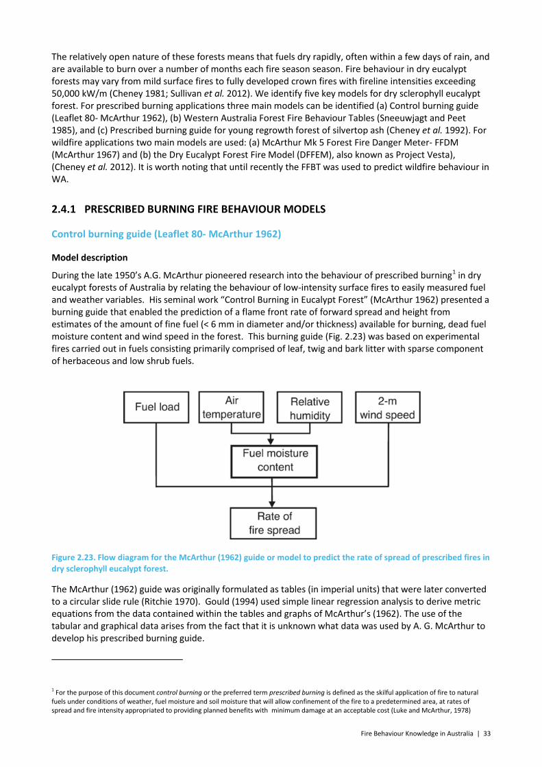
Fire Behaviour Knowledge in Australia | 33
The relatively open nature of these forests means that fuels dry rapidly, often within a few days of rain, and are available to burn over a number of months each fire season season. Fire behaviour in dry eucalypt forests may vary from mild surface fires to fully developed crown fires with fireline intensities exceeding 50,000 kW/m (Cheney 1981; Sullivan et al. 2012). We identify five key models for dry sclerophyll eucalypt forest. For prescribed burning applications three main models can be identified (a) Control burning guide (Leaflet 80- McArthur 1962), (b) Western Australia Forest Fire Behaviour Tables (Sneeuwjagt and Peet 1985), and (c) Prescribed burning guide for young regrowth forest of silvertop ash (Cheney et al. 1992). For wildfire applications two main models are used: (a) McArthur Mk 5 Forest Fire Danger Meter- FFDM (McArthur 1967) and (b) the Dry Eucalypt Forest Fire Model (DFFEM), also known as Project Vesta), (Cheney et al. 2012). It is worth noting that until recently the FFBT was used to predict wildfire behaviour in WA.
2.4.1 PRESCRIBED BURNING FIRE BEHAVIOUR MODELS
Control burning guide (Leaflet 80- McArthur 1962)
Model description
During the late 1950’s A.G. McArthur pioneered research into the behaviour of prescribed burning1
in dry eucalypt forests of Australia by relating the behaviour of low-intensity surface fires to easily measured fuel and weather variables. His seminal work “Control Burning in Eucalypt Forest” (McArthur 1962) presented a burning guide that enabled the prediction of a flame front rate of forward spread and height from estimates of the amount of fine fuel (< 6 mm in diameter and/or thickness) available for burning, dead fuel moisture content and wind speed in the forest. This burning guide (Fig. 2.23) was based on experimental fires carried out in fuels consisting primarily comprised of leaf, twig and bark litter with sparse component of herbaceous and low shrub fuels.
Figure 2.23. Flow diagram for the McArthur (1962) guide or model to predict the rate of spread of prescribed fires in dry sclerophyll eucalypt forest.
The McArthur (1962) guide was originally formulated as tables (in imperial units) that were later converted to a circular slide rule (Ritchie 1970). Gould (1994) used simple linear regression analysis to derive metric equations from the data contained within the tables and graphs of McArthur’s (1962). The use of the tabular and graphical data arises from the fact that it is unknown what data was used by A. G. McArthur to develop his prescribed burning guide.
1 For the purpose of this document control burning or the preferred term prescribed burning is defined as the skilful application of fire to natural fuels under conditions of weather, fuel moisture and soil moisture that will allow confinement of the fire to a predetermined area, at rates of spread and fire intensity appropriated to providing planned benefits with minimum damage at an acceptable cost (Luke and McArthur, 1978)

34 | Fire Behaviour Knowledge in Australia
The equations generated by Gould (1994) separate the combined effects of wind speed at 1.5 m (U1.5) and fuel moisture content (MC); from the effects of fuel load (w) slope steepness (θ). Rate of spread on level ground (R, m/min) burning a standardized fuel load (w) of 25 t ha-1 is given as:
𝑅 = 5.492 × exp (0.158 × 𝑈1.5 − 0.277 × 𝑀𝐶) [2.38]
The rate of spread is adjusted Rrf for fuel load by:
𝑅𝑟𝑓 = 0.04 × 𝑤 × 𝑅 [2.39]
Equations (2.38) and (2.39) can be combined and simplified to predict the rate of spread:
𝑅 = 0.22 × 𝑤 × exp (0.158 × 𝑈1.5 − 0.227 × 𝑀𝐶) [2.40]
Finally, rate of spread on sloping ground (𝑅𝜃) can be adjusted by:
𝑅𝜃 = 𝑅 × exp (0.0662 × 𝜃), [2.41]
where 𝜃 is the slope angle in degrees.
There was very little difference between the actual values presented in McArthur (1962) graphs and tables and the derived results from the corresponding equations (See Gould 1994, Table 3 for further details), with the fit of equations 2.38, 2.38 and 2.41 producing R2 ranging from 0.97 to 1.0. Gould (1994) points out that the equations were intended to describe McArthur’s graphs and tables as accurately as possible and it is uncertain to the goodness of fit of the equations to the original data which were not published.
Gould (1994) also derived equations from McArthur (1962) for the methods of estimating the inputs required in Eq. 2.40, namely (i) the estimation of wind speed at 1.5 m in the forest from 10-m open wind speed (or range from Beaufort wind scale), number; (ii) fuel moisture from air temperature, relative humidity and time of day; (iii) fuel load from years since last fire and canopy cover, or from litter bed depth; and (iv) fuel available for combustion from total fuel load, daily rainfall and days since last rain.
The wind speed in the forest at a 1.5 m height (U1.5, km/h) can be predicted from the 10-m open wind speed (U10, km/h) as follows:
𝑈1.5 = 1.674 + 0.1798 × (𝑈10) [2.42]
The dead fuel moisture content (%) of the surface eucalypt litter can be predicted from ambient air temperature (T, oC) and relative humidity (RH, %) taking into account expected desorption conditions between 06:00 and 12:00 h and adsorption conditions between 12:00 h onward except for two days after rainfall of 13 mm or more. For desorption conditions:
𝑀𝐶 = 12.519 + 0.112 × 𝑅𝐻 + 0.282 × 𝑇 [2.43]
For adsorption conditions:
𝑀𝐶 = 6.782 + 0.133 × 𝑅𝐻 + 0.170 × 𝑇 [2.44]
The application bounds for Equation 2.43 and 2.44 are: Temperature: 5 – 30 oC; Relative humidity: 20 – 70%.
Recent rainfall reduces the amount of fuel available for combustion and this is calculated by multiplying the fuel load (w) by a fuel reduction factor (Frf). The fuel reduction factor is calculated according to the number of days since rain (N) and the amount of rain in the last event (P, mm) as follows:
𝐹𝑟𝑓 = 0.972− 0.245 × ln(𝑃) + 0.342 × ln (𝑁) [2.45]
Model behaviour and evaluation
The McArthur (1962) burning guide was developed to assess fire behaviour potential under the low fire spread potential conditions typical of prescribed burns. The guide or model outputs do not intend to reflect the spread of a fully developed, free burning fire, but rather of a fire spreading within its built-up phase. This is reflected in the model outputs with relatively slow rates of fire spread even for low fuel moisture

Fire Behaviour Knowledge in Australia | 35
contents (e.g., <10%) and high open wind speeds. As illustrated in Fig 2.24 the model has a modest response to wind speed. Model sensitivity to fine dead fuel moisture is similar to that found in other models for fire spread in forests. The model has a directly proportional response to changes in fuel load, with a doubling in fuel load resulting in an equal change in rate of fire spread.
Davis (1976), Tolhurst et al. (1992) and Gould (1994) evaluated the predictive capacity of McArthur (1962) burning guide based on a number of operational and experimental prescribed fires. Davis (1976) compared the burning guide predictions with observed rates of spread in eight prescribed fires in dry sclerophyll forest at the Black Mountain Reserve (Australian Capital Territory). Fuel loads and observed rates of spread varied between 7 and 19 t/ha and 0.1 and 1.43 m/min, respectively. The burning guide predicted the observed rate of spread with a mean absolute error of 0.14 m/min (38%) and 0.12 m/min mean underprediction bias. Tolhurst et al. (1992) used rate of spread data from 41 prescribed burns in messmate stringybark (Eucalyptus obliqua) dominated forest located in the Wombat State Forest, Victoria. The observed rate of fire spread in this dataset varied between 0.1 and 2.5 m/min. The burning guide predictions yielded a mean absolute error of 0.26 m/min (48%) and a small underprediction mean bias of 0.1 m/min. Gould (1994) used data obtained from 37 experimental prescribed fires in young silvertop ash (Eucalyptus sieberi) regrowth forest in the south-east of New South Wales (Cheney et al. 1992). Observed rates of fire spread in this dataset varied between 0.4 and 3.9 m/min. The burning guide under-predicted 89% of cases, yielding a mean absolute error of 0.6 m/min (45%) and a mean bias of 0.6 m/min.
Figure 2.24. Prediction of rate of fire spread in eucalypt forests as a function of 10-m open wind speed and fine fuel moistures content expected to occur under prescribed burning conditions as predicted by McArthur (1962) guide or model. Flat ground and a fuel load of 25 t/ha are assumed. A wind correction factor of 3:1 is used.
Forest Fire Behaviour Tables for Western Australia - Jarrah fuel type (Sneeuwjagt and Peet 1985)
Model description
The development of formal prescribed burning guides and the practical application of prescribed burning to broad areas of forest in south-west Western Australia was initiated in 1962 under the guidance of Forests Department research officer George. B. Peet who applied techniques similiar to those developed by Alan G. McArthur to develop a fuel type-specific prescribed burning guide for northern jarrah forest (Peet 1965) (Fig. 2.25). Data came from 130 experimental fires lit in jarrah forest near Dwellingup, WA, during the

36 | Fire Behaviour Knowledge in Australia
spring and summer months over three fire seasons with a further 70 fires conducted during autumn used for evaluation purposes. Experimental fires were lit from a point and allowed to develop for periods of up to 1 hour with the perimeter marked at intervals of 4 minutes (Burrows and Sneeuwjagt 1991).
The operational expression of Peet’s work was in the form of the Forest Fire Behaviour Tables (FFBT), first issued in 1968 in distinctive red pocket-book format under the authority of the WA Conservator of Forests (Harris 1968). The tables were fully revised by Sneeuwjagt and Peet (1976) to incorporate a book-keeping system to predict surface and profile litter moisture contenst, separate rate of spread tables for karri forest, and aids for estimating fuel quantity in southern forest types. In 1985 a revised rate of fire spread model for jarrah forest was incorporated into the tables (Sneeuwjagt and Peet 1985) based on provisional analysis of the data collected by Neil Burrows from experimental fires conducted under dry summer conditions. While the tables have been re-issued with later dates dates (e.g., the latest reprinting was carried out in 1998) , the underlying models remain unchanged since 1985.
As noted earlier, Beck (1995) fitted equations to the tables and provided a comprehensive description of the structure of the various models, their application bounds, and the range of experimental data used to develop them. The FFBT also provide a range of other decision support guidance for fire management including canopy scorch height, hours of burning time available, and resource despatch levels for bushfire suppression. Further information on the development of prescribed burning guides in Western Australia is provided by Burrows and Sneeuwjagt (1991) and McCaw et al. (2003).
Figure 2.25. Flow diagram for the Sneeuwjagt and Peet (1985) FFBT model to predict the rate of fire spread in prescribed burns in eucalypt forest.
In the FFBT three variables are considered to influence rate of fire spread in flat ground, these being the moisture content of the surface litter fuels (MC), the quantity of fuel available for burning (w), and the in-forest wind speed near the ground (1.5 - 2m). These variables variables are combined to predict a fire danger index for northern jarrah forest. Surface moisture content and wind speed are first used to calculate a forward rate of headfire spread (R, m/hr), expressed as a fire danger index (FDI), for standard fuel and forest stand structural conditions that are typical of five-year-old jarrah fuels (after Beck 1995):
𝐹𝐷𝐼𝑁𝐽 = 𝑌𝐽 + 𝐴𝐽 × 𝑒𝑥𝑝�𝑈1.5 ×𝑁𝐽� [2.46]
where
𝑌𝐽 = 21.37 − 3.42 × 𝑀𝐶 + 0.085 × 𝑀𝐶2 [2.47]
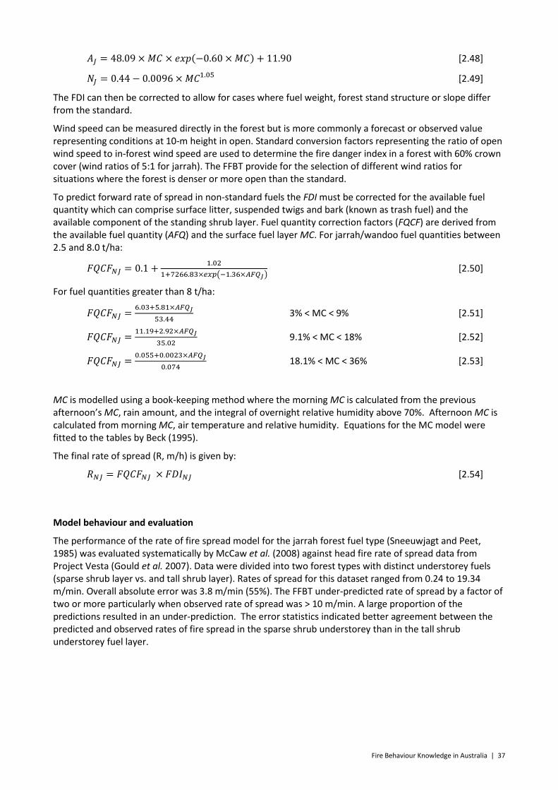
Fire Behaviour Knowledge in Australia | 37
𝐴𝐽 = 48.09 × 𝑀𝐶 × 𝑒𝑥𝑝(−0.60 × 𝑀𝐶) + 11.90 [2.48]
𝑁𝐽 = 0.44− 0.0096 × 𝑀𝐶1.05 [2.49]
The FDI can then be corrected to allow for cases where fuel weight, forest stand structure or slope differ from the standard.
Wind speed can be measured directly in the forest but is more commonly a forecast or observed value representing conditions at 10-m height in open. Standard conversion factors representing the ratio of open wind speed to in-forest wind speed are used to determine the fire danger index in a forest with 60% crown cover (wind ratios of 5:1 for jarrah). The FFBT provide for the selection of different wind ratios for situations where the forest is denser or more open than the standard.
To predict forward rate of spread in non-standard fuels the FDI must be corrected for the available fuel quantity which can comprise surface litter, suspended twigs and bark (known as trash fuel) and the available component of the standing shrub layer. Fuel quantity correction factors (FQCF) are derived from the available fuel quantity (AFQ) and the surface fuel layer MC. For jarrah/wandoo fuel quantities between 2.5 and 8.0 t/ha:
𝐹𝑄𝐶𝐹𝑁𝐽 = 0.1 + 1.021+7266.83×𝑒𝑥𝑝�−1.36×𝐴𝐹𝑄𝐽�
[2.50]
For fuel quantities greater than 8 t/ha:
𝐹𝑄𝐶𝐹𝑁𝐽 = 6.03+5.81×𝐴𝐹𝑄𝐽53.44
3% < MC < 9% [2.51]
𝐹𝑄𝐶𝐹𝑁𝐽 = 11.19+2.92×𝐴𝐹𝑄𝐽35.02
9.1% < MC < 18% [2.52]
𝐹𝑄𝐶𝐹𝑁𝐽 = 0.055+0.0023×𝐴𝐹𝑄𝐽0.074
18.1% < MC < 36% [2.53]
MC is modelled using a book-keeping method where the morning MC is calculated from the previous afternoon’s MC, rain amount, and the integral of overnight relative humidity above 70%. Afternoon MC is calculated from morning MC, air temperature and relative humidity. Equations for the MC model were fitted to the tables by Beck (1995).
The final rate of spread (R, m/h) is given by:
𝑅𝑁𝐽 = 𝐹𝑄𝐶𝐹𝑁𝐽 × 𝐹𝐷𝐼𝑁𝐽 [2.54]
Model behaviour and evaluation
The performance of the rate of fire spread model for the jarrah forest fuel type (Sneeuwjagt and Peet, 1985) was evaluated systematically by McCaw et al. (2008) against head fire rate of spread data from Project Vesta (Gould et al. 2007). Data were divided into two forest types with distinct understorey fuels (sparse shrub layer vs. and tall shrub layer). Rates of spread for this dataset ranged from 0.24 to 19.34 m/min. Overall absolute error was 3.8 m/min (55%). The FFBT under-predicted rate of spread by a factor of two or more particularly when observed rate of spread was > 10 m/min. A large proportion of the predictions resulted in an under-prediction. The error statistics indicated better agreement between the predicted and observed rates of fire spread in the sparse shrub understorey than in the tall shrub understorey fuel layer.

38 | Fire Behaviour Knowledge in Australia
Figure 2.26. Prediction of rate of fire spread in Jarrah as a function of 10-m open wind speed and fine fuel moistures content expected to occur under prescribed burning conditions according to Sneeuwjagt and Peet (1985) FFBT models. Flat ground and a fuel load of 20 t/ha are assumed. A wind correction factor of 3:1 is used (Beck 1995).
Prescribed burning guide for young regrowth forest of silvertop ash (Cheney et al. 1992)
Model description
Cheney et al. (1992) describes a study aimed at developing a prescribed burning guide for regrowth forest of silvertop ash (Eucalyptus sieberi) in the southeast of New South Wales (Fig. 2.27).
Figure 2.27. Flow diagram for the Cheney et al. (1992) model to predict the rate of spread of prescribed fires in young regrowth forests of silvertop ash.
Data on fuel, weather and fire behaviour were recorded on 56 experimental prescribed fires. The experimental fires were designed to enable measurement of the maximum headfire rate of spread possible under a range of weather conditions, slope and understorey vegetation and surface fuel loads. The most significant variables identified to influence the rate of spread (R) were wind speed at a 2-m height (U2,
range: 0 to 6 km/h), the dead fine fuel moisture content of the near-surface fuel (MC, range 10 to 24 %), the near-surface fuel percent cover, which was replaced in the analysis by the height of near-surface fuels (H, range 0.2 to 1.2 m), and the slope in the direction of the wind (𝜃, range 0 to 25 degrees).
The equation to predict the forward rate of fire spread (R, m/min) was parameterized through nonlinear regression analysis as:
𝑅 = −1.554 + 0.652 × 𝑈20.648 + 199.921 exp(−0.396 × 𝑀𝐶𝑛𝑠) + 1.61 × 𝐻𝑛𝑠 + 0.369 exp(0.062 × 𝜃) [2.55]
This equation yielded an R2 value of 0.78. Equation 2.55 has been coded into a nomogram for field estimation of rate of spread (refer to Figure 31 in Cheney et al. 1992). A MC model was not developed but
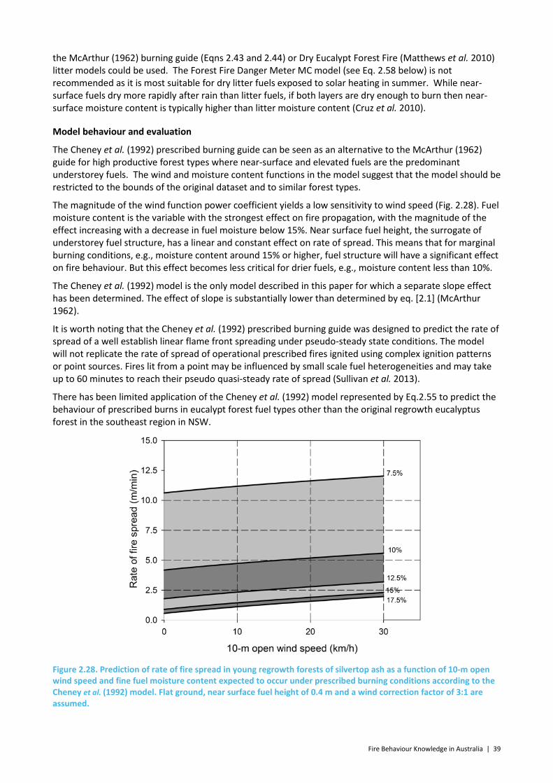
Fire Behaviour Knowledge in Australia | 39
the McArthur (1962) burning guide (Eqns 2.43 and 2.44) or Dry Eucalypt Forest Fire (Matthews et al. 2010) litter models could be used. The Forest Fire Danger Meter MC model (see Eq. 2.58 below) is not recommended as it is most suitable for dry litter fuels exposed to solar heating in summer. While near-surface fuels dry more rapidly after rain than litter fuels, if both layers are dry enough to burn then near-surface moisture content is typically higher than litter moisture content (Cruz et al. 2010).
Model behaviour and evaluation
The Cheney et al. (1992) prescribed burning guide can be seen as an alternative to the McArthur (1962) guide for high productive forest types where near-surface and elevated fuels are the predominant understorey fuels. The wind and moisture content functions in the model suggest that the model should be restricted to the bounds of the original dataset and to similar forest types.
The magnitude of the wind function power coefficient yields a low sensitivity to wind speed (Fig. 2.28). Fuel moisture content is the variable with the strongest effect on fire propagation, with the magnitude of the effect increasing with a decrease in fuel moisture below 15%. Near surface fuel height, the surrogate of understorey fuel structure, has a linear and constant effect on rate of spread. This means that for marginal burning conditions, e.g., moisture content around 15% or higher, fuel structure will have a significant effect on fire behaviour. But this effect becomes less critical for drier fuels, e.g., moisture content less than 10%.
The Cheney et al. (1992) model is the only model described in this paper for which a separate slope effect has been determined. The effect of slope is substantially lower than determined by eq. [2.1] (McArthur 1962).
It is worth noting that the Cheney et al. (1992) prescribed burning guide was designed to predict the rate of spread of a well establish linear flame front spreading under pseudo-steady state conditions. The model will not replicate the rate of spread of operational prescribed fires ignited using complex ignition patterns or point sources. Fires lit from a point may be influenced by small scale fuel heterogeneities and may take up to 60 minutes to reach their pseudo quasi-steady rate of spread (Sullivan et al. 2013).
There has been limited application of the Cheney et al. (1992) model represented by Eq.2.55 to predict the behaviour of prescribed burns in eucalypt forest fuel types other than the original regrowth eucalyptus forest in the southeast region in NSW.
Figure 2.28. Prediction of rate of fire spread in young regrowth forests of silvertop ash as a function of 10-m open wind speed and fine fuel moisture content expected to occur under prescribed burning conditions according to the Cheney et al. (1992) model. Flat ground, near surface fuel height of 0.4 m and a wind correction factor of 3:1 are assumed.

40 | Fire Behaviour Knowledge in Australia
2.4.2 WILDFIRE BEHAVIOUR MODELS
McArthur Mk 5 Forest Fire Danger Meter (FFDM) (McArthur 1967)
Model description
The development of the McArthur’s Forest Fire Danger Meters saw a number of different versions produced beginning in the early 1960’s that culminated with the publication of the Mk 4 version (McArthur 1967) and its SI units variant (known as the Mk 5) some years later (McArthur 1973). An important principle in McArthur’s approach to fire spread modelling was that fire danger and fire behaviour were intimately linked, with fire spread being directly determined from the fire danger index, a relative numerical rating.
Early development of the Forest Fire Danger Rating System in the late 1950’s was based on measured fire behaviour in experimental fires in dry sclerophyll eucalyptus forest (10-20 m tall) carrying continuous surface fuel of leaf, twig and bark litter with very little undergrowth vegetation present (McArthur 1958; McArthur and Luke 1963). Fuels were relatively uniform with a characteristic fuel load of approximately 12.5 t/ha (Cheney 1968; Cheney 1991). Each experimental fire was given a suppression difficulty rating, later redefined as fire danger classes (Cheney 1991). The difficulty-of-suppression/fire danger rating was related with the rate of spread of the head fire, the surface moisture content of the fine fuels, wind speed and fuel load. No preconceived functional relationships were assumed between these variables and best-fit curves were extrapolated to cover the weather conditions likely to occur in a typical summer in southern Australia (Noble et al. 1980).
Originally the fire danger rating was presented as a series of tables (McArthur 1958). Periodic updates to the meter aimed to incorporate the latest understanding in fire behaviour garnered from a continuously increasing number of experimental fires and documented wildfires. McArthur (1967) published the meter in circular slide rule form. The front of the meter allowed for the calculation of a Forest Fire Danger Index (FFDI) on the basis of long term drought, recent rainfall, air temperature, relative humidity, and wind speed (Fig. 2.29). The back of the meter provides tables for estimating three fire behaviour characteristics related to the FFDI, namely rate of fire spread, flame height and spotting distance. It is worth noting that limited documentation and data accompanied the development of the meter.
Figure 2.29. Flow diagram for the McArthur (1967) Forest Fire Danger Meter to predict the rate of fire spread, flame height and spotting distance in dry sclerophyll eucalypt forests.

Fire Behaviour Knowledge in Australia | 41
The tabulated indices and rate of spread values from the FFDM were converted to equations by Noble et al. (1980). The equations were derived from data taken either by measuring displacement along the scale, by taking it directly from the table on the back of the meter, or from hand-drawn graphs provided by A.G. McArthur. The FFDI function was parameterized as:
FFDI = 2.0 × exp (−0.450 + 0.987 × ln(𝐷)− 0.0345 × 𝑅ℎ + 0.0338 × 𝑇 + 0.0234 × 𝑈10) [2.56]
where D being the Drought Factor (1-10), RH is the relative humidity (%), T is the air temperature (oC) and U10 the average 10-m open wind speed (km/h).
MC is not explicitly included in the equation to calculate the FFDI, instead incorporated through T and RH. Matthews (2009) reformulated Eq. 2.56 to enable MC to be included explicitly:
𝐹𝐹𝐷𝐼 = 34.81 × 𝑒0.987×𝑙𝑛(𝐷) ×𝑀𝐶−2.1 × 𝑒0.0234 𝑈10 [2.57]
As a result, any suitable MC model for dry eucalypt litter can be utilised. McArthur (1967) included a table for predicting MC from Tair and RH which was approximated by Viney (1992) as:
𝑀𝐶 = 5.658 + 0.04651 × 𝑅𝐻 + 0.0003151 × 𝑅𝐻3 × 𝑇−1 − 0.185 × 𝑇0.77 [2.58]
The drought factor (D), a measure of the fraction of fuels available for consumption at a landscape level, was estimated as:
𝐷 = 0.191×(𝐾𝐵𝐷𝐼+104)× (𝑁+1)1.5
3.52×(𝑁+1)1.5+ 𝑃−1 [2.59]
where KBDI (mm) is the Keetch Byram Drought Index (Keetch and Byram 1968), N is the number of days since rain, and P is the amount of precipitation (mm) in the last rain event.
Noble et al. (1980) admit that the drought factor equation does not produce an exact fit to McArthur’s discontinuous (step) function used in the meter. No assessment of its performance was provided but it was considered to be suitable “for most purposes”.
Griffiths (1999) found that the values of D calculated by Noble et al. (1980) and the value determine from the FFDM for the same conditions could result in marked differences in the FFDI calculations. Griffiths found that the difference could be as much as two fire danger class ratings (e.g., Extreme vs. High). In order to provide a smooth transition of D across soil moisture deficiency boundaries, Griffiths (1999) derived a new equation for D:
𝐷 = 𝑚𝑎𝑥 �10.5 �1 − 𝑒𝑥𝑝 −(𝐼+30)40
�× 𝑦+42𝑦2+3𝑦=42
, 10� [2.60]
where the y function is calculated as follows:
𝑦 = (𝑃 − 2)/𝑁1.3, if N ≥ 1 and P > 2, [2.61]
𝑦 = (𝑃 − 2)/0.81.3 if N = 0 and P > 2, [2.62]
𝑦 = 0, if P ≤ 2. [2.63]
Finkele et al. (2006) extended this approach to develop a nationally applicable gridded forecast tool for D, comparing the effects of choice of model for the soil moisture deficiency value. They found that use of Mount’s Soil Dryness Index (Mount 1972) instead of the KBDI generally led to higher soil moisture deficits, which results in a higher drought factor, primarily due to the difference in the treatment of evapotranspiration. The review of Sullivan (2001) discussed these differences and impacts on D in some detail.
Rate of fire spread in flat ground (R, km/h) was derived by Noble et al. (1980) as:
𝑅 = 0.0012 × 𝐹𝐹𝐷𝐼 × 𝑤 [2.64]
Equations 2.56 through 2.64 are accepted as providing good estimates of the original circular FFDM slide rule values, and have been incorporated into a number of automated systems for predicting fire behaviour

42 | Fire Behaviour Knowledge in Australia
(e.g., AUSTRALIS (Johnston et al. 2009), Phoenix RAPIDFire (Tolhurst et al. 2008), SiroFire (Coleman and Sullivan 1996)).
Model behaviour and evaluation
The McArthur (1967) FFDM rate of spread component has been subject to a number of reviews and evaluation (e.g., Burrows 1991; Cheney 1991; McCaw et al. 2008). It is commonly agreed that under dry burning conditions the model will under-predict the spread rate of a wildfire propagating with a well established flame front (Burrows 1994). Cheney and Gould (1996) point out this underprediction bias to be by a factor of three or more. This is likely due to the wind function that results in moderate response to this variable under moderate to high wind speeds (Fig 2.30). This might be a result of the model being parameterized based on fires propagating in litter fuel beds where the wind effect is lower than observed in fuel complexes with a understorey dominated by near-surface and or elevated fuels. The model has a strong dead fuel moisture content effect, namely when the moisture level drops below about 6-7% (McArthur 1967; Burrows 1984). This strong effect aims to capture the contribution of profuse short range spotting that occurs at lower fuel moisture contents levels, leading to a step-chance increase in rate of fire spread (Cheney and Barry 1969; Cruz et al. 2012).
The significance of fuel complex structure is incorporated into the model through the effect of surface fuel load. As previously discussed with respect to McArthur (1962) burning, fuel load has a directly proportional effect on rate of spread, e.g., doubling in fuel load results in an equal increase in rate of fire spread. Recent research has shown that the effect of fuel load on rate of fire spread is dependent on the driving weather conditions (McCaw et al. 2012). These authors found that for dry fuel conditions, fuel load was a significant factor under low wind speeds but less significant under strong wind speed conditions. This might explain the fuel load effect found by Alan McArthur in his early experimental work.
Figure 2.30. Prediction of rate of fire spread in dry sclerophyll eucalypt forests as a function of the 10-m open wind speed and fine fuel moistures content expected to occur under wildfire conditions according to the McArthur (1967) Forest Fire Danger Meter. Flat ground and a fuel load of 25 t/ha are assumed.
The predictive capacity of the FFDM has been reported in a number of studies. We will report on the studies that had a substantial number of fires, allowing for the calculation of robust error statistics. Studies where the FFDM outputs were compared with only a few spread rate observations are not discussed here (e.g., Cheney 1968; Cruz and Plucinski 2007). We also only report on studies that compared the FFDM with fires burning under moderate or higher fire danger conditions, leaving out comparisons of the model output against prescribed burn data (e.g. Tolhurst et al. 1992).
Fire Behaviour Knowledge in Australia | 43
Burrows (1994, 1999) evaluated the predictive capacity of the FFDM against data from 35 experimental fires in WA jarrah (Eucalyptus marginata) forest of south western Australia. Rates of spread varied between 0.25 and 9.9 m/min in this dataset. The McArthur Mk 5 meter predictions had an associated mean absolute error of 1.13 m/min (56%). Sixty-six percent of the data was under-predicted, resulting in an underprediction mean bias of 0.9 m/min.
McCaw et al. (2008) evaluated the performance of the rate of fire spread component of the FFDM against headfire spread rate data from Project Vesta (Gould et al. 2007). Data was divided into two jarrah forest types with distinct understorey fuels (sparse shrub layer vs. and tall shrub layer). Rates of spread for this dataset ranged from 0.24 to 19.34 m/min. Overall absolute error was 4.0 m/min (65%). The FFDM under-predicted the rate of fire spread by a factor of two or more particularly when the observed rate of spread was > 10 m/min. Eighty-one percent of the predictions resulted in an underprediction. The error statistics indicated better agreement between the predicted and observed rates of spread in the sparse shrub understorey than in the tall shrub understorey fuel layer. The rates of spread predicted by the FFDM were closest to observed values when 10-m open winds were less than 12 km/h in the sparse shrub understorey fuel type (McCaw et al. 2008).
Kilinc et al. (in press) evaluated the performance of the FFDM against data from 181 wildfire spread rate observations obtained from southern Australia. The main fuel types in this dataset were dry sclerophyll forest with and without understorey vegetation and a few fires in more productive wet/mixed forests (n=7). Rates of fire spread in this dataset varied between 0.2 and 260 m/min. The use of the FFDM with fuel load being restricted to the original McArthur formulation, i.e., only considering litter and near surface fuels, resulted in an average absolute error of 38 m/min (86% mean error) and a significant average under-prediction bias of 37 m/min. If the fuel load was increased by the addition of the shrub and bark fuel components, the under-prediction bias was slightly reduced, but model error was still significant. For this scenario the model predictions resulted in an average absolute error of 33 m/min (100% mean error) and a significant average under-prediction bias of 28 m/min.
Overall, the FFDM might be an appropriate model to predict wildfire behaviour under mild fire weather conditions in fuel types without a significant near-surface and elevated fuel layers. The model might be appropriate also to conduct simulations for early breakout phases of the fire, i.e., while the fire is spreading in a build up phase, and has not yet reached its pseudo-steady state propagation. Nonetheless, it is not know how well the model will perform under these conditions.
Dry Eucalypt Forest Fire Model (also known as Project Vesta model, Cheney et al. 2012)
Model description
Project Vesta aimed to investigate the behaviour of moderate to high-intensity fires in dry eucalypt forest under conditions of moderate to high forest fire danger (Cheney et al. 1998; Gould et al. 2007a) to address issues arising from observations of poor performance of the FFDM, apparent lack of effect of fuel load on observed rates of spread, and develop a new model for fire behaviour in dry eucalypt forest for summer conditions. This project was conducted in south-western Western Australia during the summers of 1998, 1999 and 2001 at two sites in eucalypt forest comprised of jarrah (Eucalyptus marginata) and marri (Corymbia calophylla) with top heights of 25-30 m in which prescribed burning had been used to manipulate fuel age from 2 to 22 years. The two sites had contrasting understorey fuel structures of tall and low shrubs that had developed since the last fire. The design and execution of these experiments are described in Gould et al. (2007a). The methods of fuel sampling and numerical ratings to describe the structure of the fuel complex at different ages are presented in Gould et al. (2011); and the significance of fuel and wind variables in describing fire behaviour are presented in McCaw et al. (2012).
Experimental fires were lit along a line 120 m long and designed to enable the fires to spread almost immediately at close to their potential rate of spread for the prevailing conditions (i.e. no development phase). A total of 98 experimental fires were carried out. The following range in fire weather variables was obtained for model development purposes: 10-m open wind speed: 7.3 to 26 km/h; air temperature: 21 – 32.5 °C; relative humidity 17 – 54%. Fine dead fuel moisture content in turn ranged from 5.6 to 9.6%. The
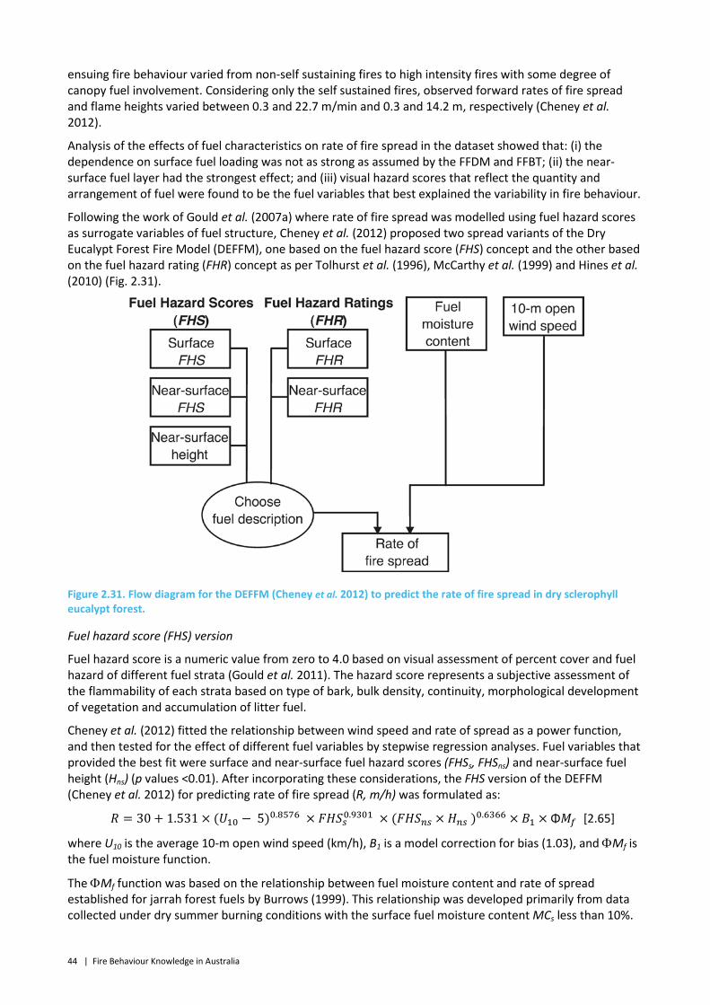
44 | Fire Behaviour Knowledge in Australia
ensuing fire behaviour varied from non-self sustaining fires to high intensity fires with some degree of canopy fuel involvement. Considering only the self sustained fires, observed forward rates of fire spread and flame heights varied between 0.3 and 22.7 m/min and 0.3 and 14.2 m, respectively (Cheney et al. 2012).
Analysis of the effects of fuel characteristics on rate of fire spread in the dataset showed that: (i) the dependence on surface fuel loading was not as strong as assumed by the FFDM and FFBT; (ii) the near-surface fuel layer had the strongest effect; and (iii) visual hazard scores that reflect the quantity and arrangement of fuel were found to be the fuel variables that best explained the variability in fire behaviour.
Following the work of Gould et al. (2007a) where rate of fire spread was modelled using fuel hazard scores as surrogate variables of fuel structure, Cheney et al. (2012) proposed two spread variants of the Dry Eucalypt Forest Fire Model (DEFFM), one based on the fuel hazard score (FHS) concept and the other based on the fuel hazard rating (FHR) concept as per Tolhurst et al. (1996), McCarthy et al. (1999) and Hines et al. (2010) (Fig. 2.31).
Figure 2.31. Flow diagram for the DEFFM (Cheney et al. 2012) to predict the rate of fire spread in dry sclerophyll eucalypt forest.
Fuel hazard score (FHS) version
Fuel hazard score is a numeric value from zero to 4.0 based on visual assessment of percent cover and fuel hazard of different fuel strata (Gould et al. 2011). The hazard score represents a subjective assessment of the flammability of each strata based on type of bark, bulk density, continuity, morphological development of vegetation and accumulation of litter fuel.
Cheney et al. (2012) fitted the relationship between wind speed and rate of spread as a power function, and then tested for the effect of different fuel variables by stepwise regression analyses. Fuel variables that provided the best fit were surface and near-surface fuel hazard scores (FHSs, FHSns) and near-surface fuel height (Hns) (p values <0.01). After incorporating these considerations, the FHS version of the DEFFM (Cheney et al. 2012) for predicting rate of fire spread (R, m/h) was formulated as:
𝑅 = 30 + 1.531 × (𝑈10 − 5)0.8576 × 𝐹𝐻𝑆𝑠0.9301 × (𝐹𝐻𝑆𝑛𝑠 × 𝐻𝑛𝑠 )0.6366 × 𝐵1 × Φ𝑀𝑓 [2.65]
where U10 is the average 10-m open wind speed (km/h), B1 is a model correction for bias (1.03), and ΦMf is the fuel moisture function.
The ΦMf function was based on the relationship between fuel moisture content and rate of spread established for jarrah forest fuels by Burrows (1999). This relationship was developed primarily from data collected under dry summer burning conditions with the surface fuel moisture content MCs less than 10%.
Fire Behaviour Knowledge in Australia | 45
Burrows (1999) suggested a power function to best describe the damping effect of dead fuel moisture of the fire spread rate:
Φ𝑀𝑓 = 18.35 × 𝑀𝐶−1.495 [2.66]
MC is taken from tables in Gould et al. (2007b) which may be approximated by
𝑀𝐶 = � 2.76 + 0.124 × 𝑅𝐻 − 0.0187 × 𝑇 Period 13.60 + 0.169 × 𝑅𝐻 − 0.0450 × 𝑇 Period 23.08 + 0.198 × 𝑅𝐻 − 0.0483 × 𝑇 Period 3
� [2.67]
where Period 1 extending from 12:00-17:00 (Daylight savings) for sunny afternoons from October to March, Period 2 is used otherwise for daylight hours, and period 3 is applicable for night-time hours.
Fuel hazard rating (FHR) version
A number of field guides have been developed to provide a systematic method for assessing a fuel hazard rating (FHR) and suppression difficulty in dry eucalypt forest (Wilson 1992, 1993; Tolhurst et al. 1996; McCarthy et al. 1999; DEH 2006; Hines et al. 2010). These guides provide a description for each fuel stratum and attributes to assess the fuel hazard into five rating classes (Low, Moderate, High, Very High and Extreme) according to what is commonly known as the Overall Fuel Hazard Guide (McCarthy et al. 1999; Hines et al. 2010).
The surface and near-surface visual fuel hazard scores from the original experimental data (Gould et al. 2007b, 2011) were allocated into five categorical hazard ratings: FHR = 1 (Low, FHS ≤ 1.5), FHR = 2 (Moderate, FHS > 1.5 and ≤ 2.5), FHR = 3 (High, FHS > 2.5 and FHS ≤ 3.5), FHR = 4 (Very High, FHS > 3.5 and ≤ 3.75) and FHR = 5 (Extreme, FHS > 3.75). The rate of fire spread (R, m/h) model using FHR values as fuel descriptors took the form:
𝑅 = 30 + 2.311 × (𝑈10 − 5)0.8364 × 𝑒𝑥𝑝�∑ 𝑏2,𝑖(𝐼𝑠)𝑖 + ∑ 𝑏3,𝑖(𝐼𝑛𝑠)𝑖5𝑖=2
5𝑖=2 � × 𝐵2 × Φ𝑀𝑓 [2.68]
where Is and Ins are indicator variables for surface and near-surface fuel categories respectively (so, for example, (Is)i = 1 if the surface fuel hazard rating is i, and zero otherwise). The regression fuel coefficients for this equation are given in Table 2.5. The B2 value in the model is the correction for bias of 1.02. The ΦMf is the fuel moisture function as described in Eq. 2.66 .
Table 2.5. Surface and near-surface fuel hazard rating regression coefficients for the fuel hazard rating (FHR) version of the rate of fire spread model of Cheney et al. (2012).
REGRESSION CONSTANTS ESTIMATE Surface fuel b22 1.5608 b23 2.1412 b24 2.0548 b25 2.3251 Near-surface fuel b31 0.4694 b32 0.7070 b33 1.2772 b34 1.7492 b35 1.2446
Model behaviour and evaluation
The functional forms used in DEFFM (Cheney et al. 2012) reflect the accrued understanding of the effects of environmental and fuel variables on rate of fire spread and fire behaviour in general. The bulk effect of wind speed was modelled using a power law function with an exponent close to 1, resulting in an approximately linear effect (Fig 2.32). The fuel moisture content effect relies on a power function that approaches an exponential decay with a notable higher effect for low fuel moistures (Fig 2.32). This effect

46 | Fire Behaviour Knowledge in Australia
reflects a nonlinear aspect of fire propagation in eucalypt forests, where under dry conditions the onset of mass spotting behaviour result in substantial increases in rate of fire spread.
Fuel structure is incorporated into the model though descriptors of the surface (FHS) and near-surface (FHS and height) fuel layers. The surface FHS has a slight higher effect on rate of spread than the near surface FHS. A variation of surface FHS from 1 to 4 will result in an approximate three-fold increase in the rate of fire spread. The same change in the near-surface FHS result in a x2.3 increase in rate of spread. The model is also sensitive to the height of the near surface fuel layer. A doubling of the near surface height will result in a 65% increase in the rate of fire spread. Model sensitivity to the near-surface fuel height warrants special care in its estimation. Measurement errors in the definition of this layer can result in significant bias in the model output (e.g., including part of the elevated fuels in the near surface layer; considering top height instead of average height, not sampling enough points).
Figure 2.32. prediction of rate of fire spread in dry sclerophyll eucalypt forests in (a) young and (b) old fuels as a function of 10-m open wind speed and fine fuel moistures content expected to occur under wildfire conditions according to the FHS version of the DEFFM (Cheney et al. 2012). Flat ground is assumed. Young fuels are described as: Surface FHS of 2; Near surface FHS of 1.5; and near surface fuel height of 0.15 m. Old fuels are described as: Surface FHS of 3.5; Near surface FHS of 3; near surface fuel height of 0.25 m.

Fire Behaviour Knowledge in Australia | 47
The DEFFM rate of fire spread models were evaluated against independent fire spread data compiled from experimental fires and from well-documented wildfires in open eucalypt forests in southern Australia (Cheney et al. 2012). The wildfire dataset had fires burning under higher wind speeds, lower dead fuel moisture contents and in fuel types other than those where the project Vesta experimental fires were conducted in south-west Western Australia. The experimental fires had spread rates ranging from 2.5 to 16 m/min. Rate of spread in the wildfire dataset varied between 10 and 175 m/min. Overall, the models predicted the experimental fire data with an average absolute error of 2.2 m/min, which equates to a percent error of 35%. Bias was negligible at 0.03 m/min. For the wildfire dataset the mean absolute error was 26.4 m/min (54% error). The increase in error is possibly due to the larger uncertainty regarding the weather conditions at the fire location and difficulties in obtaining accurate measurements of the rate of wildfire propagation. The model tended to over-predict the spread of the wildfires, with 68% of the cases in this class and a mean bias of -6.8 m/min (approximately 25% of the mean error). Overall the goodness of fit statistics were slightly better with the FHR rate of fire spread model than with FHS model.
Kilinc et al. (in press) evaluated the performance of the DEFFM models against wildfire data from southern Australia. The FHS and FHR versions performed with similar statistics, with average errors between 25 and 23 m/min respectively. Both models predicted the dataset with residual bias (< 1 m/min for FHS and 5 m/min for FHR).
2.5 Wet Eucalypt forests
Forest Fire Behaviour Tables for Western Australia – Karri fuel type (Sneeuwjagt and Peet 1985)
Model description
The above described Forest Fire Behaviour Tables (FFBT) incorporate a section allowing the prediction fire behaviour in Western Australia Karri forest. Beck (1995) fitted equations to the Karri tables and provided a comprehensive description of the structure of the various models, their application bounds, and the range of experimental data used to develop them. As per the Jarrah model, four variables are considered to influence rate of spread: the moisture content of the surface litter fuels (MC), the quantity of fuel available for burning (w), the in-forest wind speed near the ground (1.5 - 2m) and the slope of the terrain. The fire danger index for karri forests assumes a medium-density understorey of shrubs 3.5-5.5 m tall (referred to as Type 4 & 5). Surface moisture content and wind speed are first used to calculate a forward rate of headfire spread (R, m/hr), expressed as a fire danger index (FDI), for a typical forest structure with five-year-old karri fuels (After Beck 1995):
𝐹𝐷𝐼𝐾 = 𝑌𝐾 + 𝐴𝐾 × 𝑒𝑥𝑝(𝑈1.5 × 𝑁𝐾) [2.69]
where
𝑌𝐾 = 4.88 − 263.78 × 𝑀𝐶1.8 [2.70]
𝐴𝐾 = 163.40 × 𝑀𝐶−1.18 [2.71]
𝑁𝐾 = 0.54− 0.0059 × 𝑀𝐶 [2.72]
This spread rate/fire danger index value is then corrected to allow for cases where fuel weight, forest stand structure or slope differ from the standard. As per for the Jarrah model, wind speed can be measured directly in the forest but is more commonly a forecast or observed value representing conditions at 10 m height in open exposure. The standard conversion for karri forest is 7:1. (Sneeuwjagt and Peet 1985) provide tables for selection of different wind ratios for situations where the forest is denser or more open than the standard.
To predict forward rate of spread in non-standard fuels the fire danger index must be corrected for the available fuel quantity which can comprise surface litter, suspended twigs and bark (known as trash fuel) and the available component of the standing shrub layer. Fuel quantity correction factors (FQCF) are

48 | Fire Behaviour Knowledge in Australia
derived from the available fuel quantity (AFQ) and the moisture content of the surface fuel layer (MC). For karri fuel types fuel quantities between 5.0 and 17.0 t/ha:
𝐹𝑄𝐶𝐹𝐾 = 0.16 + 0.951+957.74×𝑒𝑥𝑝�−0.52×𝐴𝐹𝑄𝐽�
[2.73]
For fuel quantities higher than 17.0 t/ha:
𝐹𝑄𝐶𝐹𝐾 = 5.08+6.26×𝐴𝐹𝑄𝐽111.50
3% < MC < 9.9% [2.74]
𝐹𝑄𝐶𝐹𝐾 = 17.35+1.70×𝐴𝐹𝑄𝐽46.25
10% < MC < 18.9% [2.75]
𝐹𝑄𝐶𝐹𝐾 = 10.88+0.46×𝐴𝐹𝑄𝐽18.7
18.9% < MC < 26% [2.76]
MC is modelled using a book-keeping method where morning MC is calculated from the previous afternoon’s MC, rain amount, and the integral of overnight RH above 70%. Afternoon MC is calculated from morning MC, T and RH. Equations for the MC model were fitted to the tables by Beck (1995).
The final rate of spread (R, m/h) is given by:
𝑅𝐾 = 𝐹𝑄𝐶𝐹𝐾 × 𝐹𝐷𝐼𝐾 [2.77]
Model behaviour and evaluation
The karri forest fire behaviour predictions from the FFBT relate to surface fires and are intended primarily as a guide to prescribed burning. For the same burning conditions, the karri rate of fire spread model (Fig . 2.33) will predict slower and lower intensity fires than obtained for jarrah forests. The results are comparable to those obtained for the McArthur (1962) burning guide although with some departures due to the distinct functional forms used in model parameterization. We are presently unaware of any published evaluation on the performance of the karri fire spread model against independent datasets..
Figure 2.33. Rate of fire spread in Karri forests as a function of 10-m open wind speed and fine fuel moistures content expected to occur under prescribed burning conditions according to Sneeuwjagt and Peet (1985) FFBT model. Flat ground, fuel load of 20 t/ha and a wind correction 6:1 (Beck 1995) are assumed.
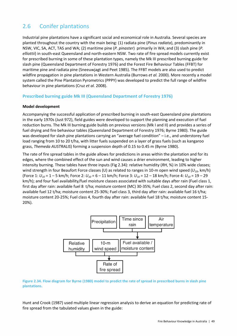
Fire Behaviour Knowledge in Australia | 49
2.6 Conifer plantations
Industrial pine plantations have a significant social and economical role in Australia. Several species are planted throughout the country with the main being: (1) radiata pine (Pinus radiata), predominantly in NSW, VIC, SA, ACT, TAS and WA; (2) maritime pine (P. pinaster) primarily in WA; and (3) slash pine (P. elliottii) in south-east Queensland and north-eastern NSW. Two rate of fire spread models currently exist for prescribed burning in some of these plantation types, namely the Mk III prescribed burning guide for slash pine (Queensland Department of Forestry 1976) and the Forest Fire Behaviour Tables (FFBT) for maritime pine and radiata pine (Sneeuwjagt and Peet 1985). The FFBT models are also used to predict wildfire propagation in pine plantations in Western Australia (Burrows et al. 2000). More recently a model system called the Pine Plantation Pyrometrics (PPPY) was developed to predict the full range of wildfire behaviour in pine plantations (Cruz et al. 2008).
Prescribed burning guide Mk III (Queensland Department of Forestry 1976)
Model development
Accompanying the successful application of prescribed burning in south-east Queensland pine plantations in the early 1970s (Just 972), field guides were developed to support the planning and execution of fuel reduction burns. The Mk III burning guide builds on previous versions (Mk I and II) and provides a series of fuel drying and fire behaviour tables (Queensland Department of Forestry 1976; Byrne 1980). The guide was developed for slash pine plantations carrying an “average fuel condition” – i.e., and understorey fuel load ranging from 10 to 20 t/ha, with litter fuels suspended on a layer of grass fuels (such as kangaroo grass, Themeda AUSTRALIS) forming a suspension depth of 0.15 to 0.45 m (Byrne 1980).
The rate of fire spread tables in the guide allows for predictions in areas within the plantation and for its edges, where the combined effect of the sun and wind causes a drier environment, leading to higher intensity burning. These tables have three inputs (Fig 2.34): relative humidity (RH, %) in 10% wide classes; wind strength in four Beaufort Force classes (U) as related to ranges in 10-m open wind speed (U10, km/h) (Force 1: U10 = 1 – 5 km/h; Force 2: U10 = 6 – 11 km/h; Force 3: U10 = 12 – 18 km/h; Force 4: U10 = 19 – 29 km/h); and four fuel availability/fuel moisture classes associated with suitable days after rain (Fuel class 1, first day after rain: available fuel 8 t/ha; moisture content (MC) 30-35%; Fuel class 2, second day after rain: available fuel 12 t/ha; moisture content 25-30%; Fuel class 3, third day after rain: available fuel 16 t/ha; moisture content 20-25%; Fuel class 4, fourth day after rain: available fuel 18 t/ha; moisture content 15-20%).
Figure 2.34. Flow diagram for Byrne (1980) model to predict the rate of spread in prescribed burns in slash pine plantations.
Hunt and Crook (1987) used multiple linear regression analysis to derive an equation for predicting rate of fire spread from the tabulated values given in the guide:
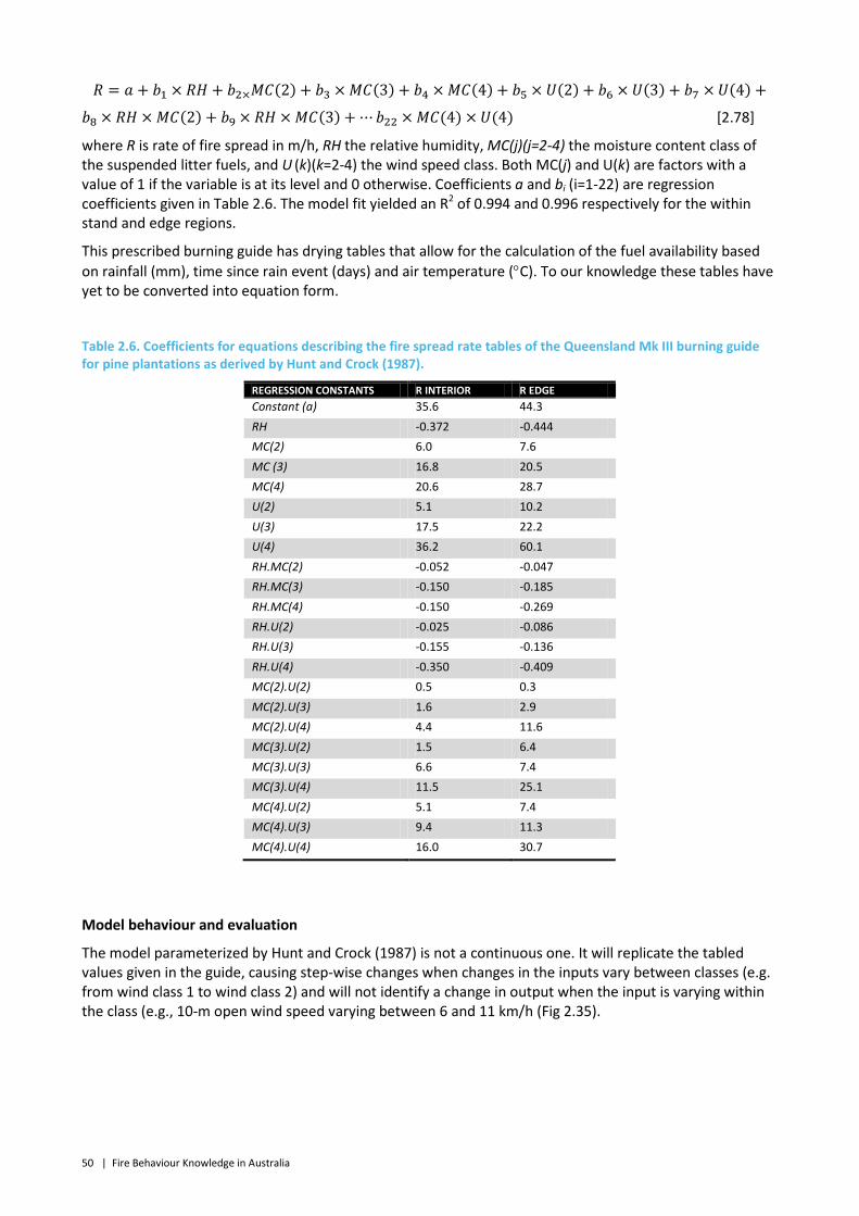
50 | Fire Behaviour Knowledge in Australia
𝑅 = 𝑎 + 𝑏1 × 𝑅𝐻 + 𝑏2×𝑀𝐶(2) + 𝑏3 × 𝑀𝐶(3) + 𝑏4 × 𝑀𝐶(4) + 𝑏5 × 𝑈(2) + 𝑏6 × 𝑈(3) + 𝑏7 × 𝑈(4) +
𝑏8 × 𝑅𝐻 × 𝑀𝐶(2) + 𝑏9 × 𝑅𝐻 × 𝑀𝐶(3) + ⋯𝑏22 × 𝑀𝐶(4) × 𝑈(4) [2.78]
where R is rate of fire spread in m/h, RH the relative humidity, MC(j)(j=2-4) the moisture content class of the suspended litter fuels, and U (k)(k=2-4) the wind speed class. Both MC(j) and U(k) are factors with a value of 1 if the variable is at its level and 0 otherwise. Coefficients a and bi (i=1-22) are regression coefficients given in Table 2.6. The model fit yielded an R2 of 0.994 and 0.996 respectively for the within stand and edge regions.
This prescribed burning guide has drying tables that allow for the calculation of the fuel availability based on rainfall (mm), time since rain event (days) and air temperature (°C). To our knowledge these tables have yet to be converted into equation form.
Table 2.6. Coefficients for equations describing the fire spread rate tables of the Queensland Mk III burning guide for pine plantations as derived by Hunt and Crock (1987).
REGRESSION CONSTANTS R INTERIOR R EDGE Constant (a) 35.6 44.3 RH -0.372 -0.444 MC(2) 6.0 7.6 MC (3) 16.8 20.5 MC(4) 20.6 28.7 U(2) 5.1 10.2 U(3) 17.5 22.2 U(4) 36.2 60.1 RH.MC(2) -0.052 -0.047 RH.MC(3) -0.150 -0.185 RH.MC(4) -0.150 -0.269 RH.U(2) -0.025 -0.086 RH.U(3) -0.155 -0.136 RH.U(4) -0.350 -0.409 MC(2).U(2) 0.5 0.3 MC(2).U(3) 1.6 2.9 MC(2).U(4) 4.4 11.6 MC(3).U(2) 1.5 6.4 MC(3).U(3) 6.6 7.4 MC(3).U(4) 11.5 25.1 MC(4).U(2) 5.1 7.4 MC(4).U(3) 9.4 11.3 MC(4).U(4) 16.0 30.7
Model behaviour and evaluation
The model parameterized by Hunt and Crock (1987) is not a continuous one. It will replicate the tabled values given in the guide, causing step-wise changes when changes in the inputs vary between classes (e.g. from wind class 1 to wind class 2) and will not identify a change in output when the input is varying within the class (e.g., 10-m open wind speed varying between 6 and 11 km/h (Fig 2.35).
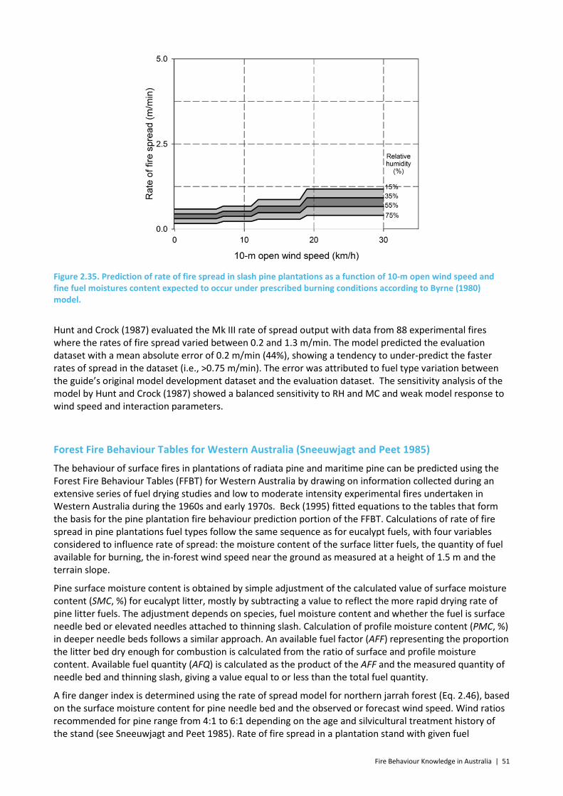
Fire Behaviour Knowledge in Australia | 51
Figure 2.35. Prediction of rate of fire spread in slash pine plantations as a function of 10-m open wind speed and fine fuel moistures content expected to occur under prescribed burning conditions according to Byrne (1980) model.
Hunt and Crock (1987) evaluated the Mk III rate of spread output with data from 88 experimental fires where the rates of fire spread varied between 0.2 and 1.3 m/min. The model predicted the evaluation dataset with a mean absolute error of 0.2 m/min (44%), showing a tendency to under-predict the faster rates of spread in the dataset (i.e., >0.75 m/min). The error was attributed to fuel type variation between the guide’s original model development dataset and the evaluation dataset. The sensitivity analysis of the model by Hunt and Crock (1987) showed a balanced sensitivity to RH and MC and weak model response to wind speed and interaction parameters.
Forest Fire Behaviour Tables for Western Australia (Sneeuwjagt and Peet 1985)
The behaviour of surface fires in plantations of radiata pine and maritime pine can be predicted using the Forest Fire Behaviour Tables (FFBT) for Western Australia by drawing on information collected during an extensive series of fuel drying studies and low to moderate intensity experimental fires undertaken in Western Australia during the 1960s and early 1970s. Beck (1995) fitted equations to the tables that form the basis for the pine plantation fire behaviour prediction portion of the FFBT. Calculations of rate of fire spread in pine plantations fuel types follow the same sequence as for eucalypt fuels, with four variables considered to influence rate of spread: the moisture content of the surface litter fuels, the quantity of fuel available for burning, the in-forest wind speed near the ground as measured at a height of 1.5 m and the terrain slope.
Pine surface moisture content is obtained by simple adjustment of the calculated value of surface moisture content (SMC, %) for eucalypt litter, mostly by subtracting a value to reflect the more rapid drying rate of pine litter fuels. The adjustment depends on species, fuel moisture content and whether the fuel is surface needle bed or elevated needles attached to thinning slash. Calculation of profile moisture content (PMC, %) in deeper needle beds follows a similar approach. An available fuel factor (AFF) representing the proportion the litter bed dry enough for combustion is calculated from the ratio of surface and profile moisture content. Available fuel quantity (AFQ) is calculated as the product of the AFF and the measured quantity of needle bed and thinning slash, giving a value equal to or less than the total fuel quantity.
A fire danger index is determined using the rate of spread model for northern jarrah forest (Eq. 2.46), based on the surface moisture content for pine needle bed and the observed or forecast wind speed. Wind ratios recommended for pine range from 4:1 to 6:1 depending on the age and silvicultural treatment history of the stand (see Sneeuwjagt and Peet 1985). Rate of fire spread in a plantation stand with given fuel
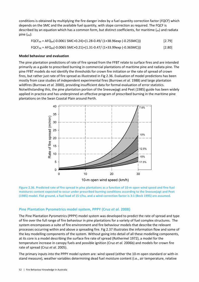
52 | Fire Behaviour Knowledge in Australia
conditions is obtained by multiplying the fire danger index by a fuel quantity correction factor (FQCF) which depends on the SMC and the available fuel quantity, with slope correction as required. The FQCF is described by an equation which has a common form, but distinct coefficients, for maritime (PP) and radiata pine (PR):
FQCFPP = AFQPP(-0.0061 SMC+0.24)+(1.28-0.49/ (1+38.96exp (-0.25SMC))) [2.79]
FQCFPR = AFQPR(-0.0065 SMC+0.21)+(1.31-0.47/ (1+33.99exp (-0.36SMC))) [2.80]
Model behaviour and evaluation
The pine plantation predictions of rate of fire spread from the FFBT relate to surface fires and are intended primarily as a guide to prescribed burning in commercial plantations of maritime pine and radiata pine. The pine FFBT models do not identify the thresholds for crown fire initiation or the rate of spread of crown fires, but rather just rate of fire spread as illustrated in Fig 2.36. Evaluation of model predictions has been mostly from case studies of independent experimental fires (Burrows et al. 1988) and large plantation wildfires (Burrows et al. 2000), providing insufficient data for formal evaluation of error statistics. Notwithstanding this, the pine plantation portion of the Sneeuwjagt and Peet (1985) guide has been widely applied in practice and has underpinned an effective program of prescribed burning in the maritime pine plantations on the Swan Coastal Plain around Perth.
Figure 2.36. Predicted rate of fire spread in pine plantations as a function of 10-m open wind speed and fine fuel moistures content expected to occur under prescribed burning conditions according to the Sneeuwjagt and Peet (1985) model. Flat ground, a fuel load of 15 t/ha, and a wind correction factor is 3:1 (Beck 1995) are assumed.
Pine Plantation Pyrometrics model system, PPPY (Cruz et al. 2008)
The Pine Plantation Pyrometrics (PPPY) model system was developed to predict the rate of spread and type of fire over the full range of fire behaviour in pine plantations for a variety of fuel complex structures. The system encompasses a suite of fire environment and fire behaviour models that describe the relevant processes occurring within and above a spreading fire. Fig 2.37 illustrates the information flow and some of the key modelling components of the system. Without going into detail of all these modelling components, at its core is a model describing the surface fire rate of spread (Rothermel 1972), a model for the temperature increase in canopy fuels and possible ignition (Cruz et al. 2006b) and models for crown fire rate of spread (Cruz et al. 2005).
The primary inputs into the PPPY model system are: wind speed (either the 10-m open standard or with-in stand measure), weather variables determining dead fuel moisture content (i.e., air temperature, relative
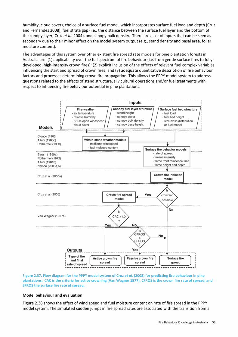
Fire Behaviour Knowledge in Australia | 53
humidity, cloud cover), choice of a surface fuel model, which incorporates surface fuel load and depth (Cruz and Fernandes 2008), fuel strata gap (i.e., the distance between the surface fuel layer and the bottom of the canopy layer; Cruz et al. 2004), and canopy bulk density. There are a set of inputs that can be seen as secondary due to their minor effect on the model system output (e.g., stand density and basal area, foliar moisture content).
The advantages of this system over other existent fire spread rate models for pine plantation forests in Australia are: (1) applicability over the full spectrum of fire behaviour (i.e. from gentle surface fires to fully-developed, high-intensity crown fires); (2) explicit inclusion of the effects of relevant fuel complex variables influencing the start and spread of crown fires; and (3) adequate quantitative description of fire behaviour factors and processes determining crown fire propagation. This allows the PPPY model system to address questions related to the effects of stand structure, silvicultural operations and/or fuel treatments with respect to influencing fire behaviour potential in pine plantations.
Figure 2.37. Flow diagram for the PPPY model system of Cruz et al. (2008) for predicting fire behaviour in pine plantations. CAC is the criteria for active crowning (Van Wagner 1977), CFROS is the crown fire rate of spread, and SFROS the surface fire rate of spread.
Model behaviour and evaluation
Figure 2.38 shows the effect of wind speed and fuel moisture content on rate of fire spread in the PPPY model system. The simulated sudden jumps in fire spread rates are associated with the transition from a
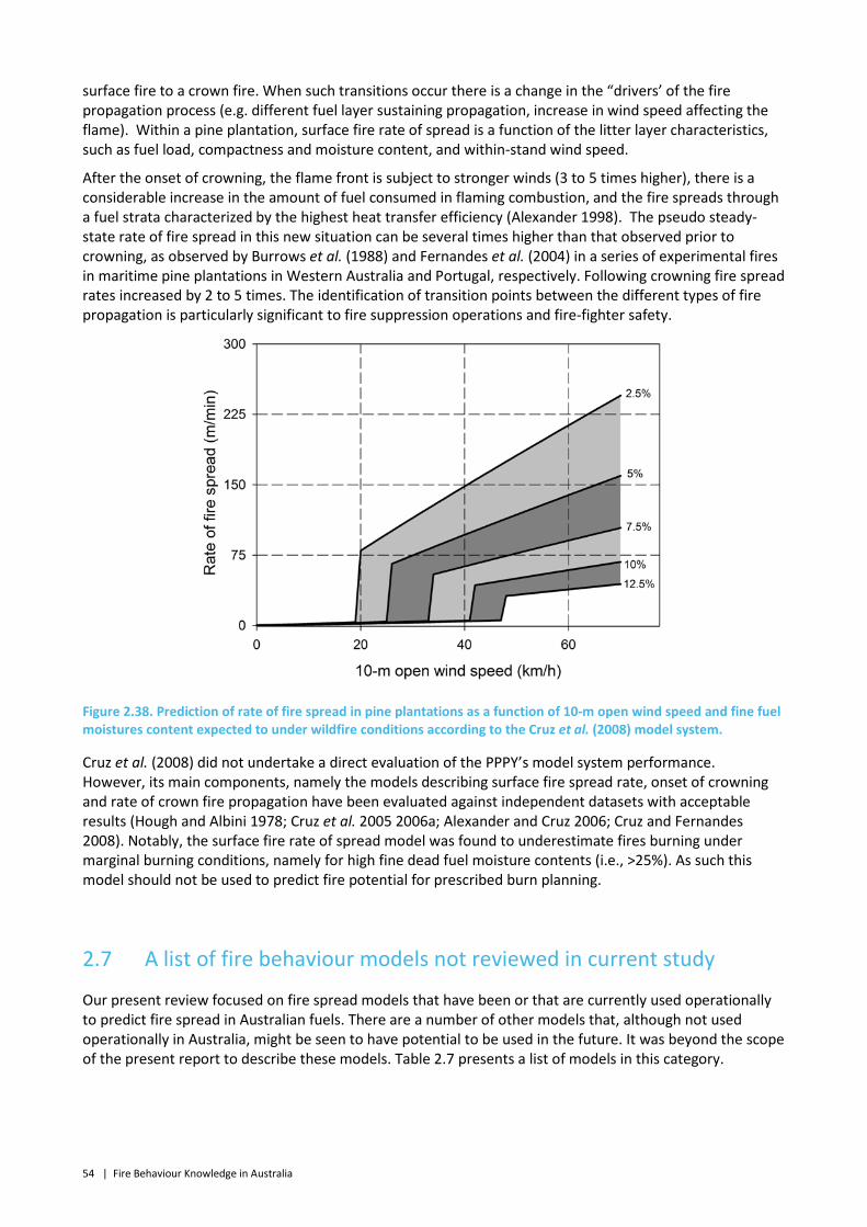
54 | Fire Behaviour Knowledge in Australia
surface fire to a crown fire. When such transitions occur there is a change in the “drivers’ of the fire propagation process (e.g. different fuel layer sustaining propagation, increase in wind speed affecting the flame). Within a pine plantation, surface fire rate of spread is a function of the litter layer characteristics, such as fuel load, compactness and moisture content, and within-stand wind speed.
After the onset of crowning, the flame front is subject to stronger winds (3 to 5 times higher), there is a considerable increase in the amount of fuel consumed in flaming combustion, and the fire spreads through a fuel strata characterized by the highest heat transfer efficiency (Alexander 1998). The pseudo steady-state rate of fire spread in this new situation can be several times higher than that observed prior to crowning, as observed by Burrows et al. (1988) and Fernandes et al. (2004) in a series of experimental fires in maritime pine plantations in Western Australia and Portugal, respectively. Following crowning fire spread rates increased by 2 to 5 times. The identification of transition points between the different types of fire propagation is particularly significant to fire suppression operations and fire-fighter safety.
Figure 2.38. Prediction of rate of fire spread in pine plantations as a function of 10-m open wind speed and fine fuel moistures content expected to under wildfire conditions according to the Cruz et al. (2008) model system.
Cruz et al. (2008) did not undertake a direct evaluation of the PPPY’s model system performance. However, its main components, namely the models describing surface fire spread rate, onset of crowning and rate of crown fire propagation have been evaluated against independent datasets with acceptable results (Hough and Albini 1978; Cruz et al. 2005 2006a; Alexander and Cruz 2006; Cruz and Fernandes 2008). Notably, the surface fire rate of spread model was found to underestimate fires burning under marginal burning conditions, namely for high fine dead fuel moisture contents (i.e., >25%). As such this model should not be used to predict fire potential for prescribed burn planning.
2.7 A list of fire behaviour models not reviewed in current study
Our present review focused on fire spread models that have been or that are currently used operationally to predict fire spread in Australian fuels. There are a number of other models that, although not used operationally in Australia, might be seen to have potential to be used in the future. It was beyond the scope of the present report to describe these models. Table 2.7 presents a list of models in this category.

Fire Behaviour Knowledge in Australia | 55
Table 2.7. Listing of models not described in the report that might provide useful fire behaviour predictions to Australian fuel complexes. Note: List is not comprehensive.
MODEL COMMENT McArthur (1963) Fire behaviour and burning guide for Brigalow lands in Queensland. Allows for the
calculation of rate of fire spread from a number of tables and graphs. Results not transformed into equations.
Rothermel (1972) Model implemented in US Fire Behaviour Prediction System, such in BEHAVE Plus (Andrews et al. 2008) and FARSITE (Finney 2004). Tested in Australian fuel complexes with mixed results. Model performed adequately in shrubland fuel complexes (e.g., McCaw 1997) but poorly in Eucalypt forests (Moore 1986; Burrows 1994).
Cheney and Just (1974) Burning guide for sugar cane plantations. This is not a fire spread model per se, but a burning guide that allows the determination of a Cane Burning Index and associated cane burning operations.
Forestry Canada Fire Danger Group (1992)
Canadian Fire Behaviour Prediction System; Implemented in Prometheus fire spread simulator and basis for NZ Fire Danger Rating System. This is a fuel type specific system parameterized for Canadian fuel complexes. Overall most Canadian fuel types have no match to Australian ones with the exception of Fuel type C-6 Conifer Plantation, which might be used to predict fire propagation in certain stages of pine plantation rotation (see NZFDRS (Pearce et al. (2012) and Cruz and Plucinski 2007). See Taylor and Alexander (2006) and Wotton et al. (2009) for updates to the system.
Buckley (1993) Burning guide for regrowth forests with wiregrass understory.
Lacy (2008) Burning guide for Young tropical eucalypt plantations with dense grassy understorey. Rate of spread model provided in this study restricted to no-wind conditions.
Leonard (2009) Fire sustainability model for grasslands. Experimental design, namely small burn plots, limits applicability of results to real world situation.
Zylstra (2011) Fire spread model developed from simplified geometrical considerations and small scale bench-top experiments. Model performance unknown.
2.8 The Practice of Predicting Bushfire Behaviour2
At its most basic level, given a fire ignition and a specified set of fuel, weather, and topographic conditions, the ultimate goal of bushfire fire research is to provide relatively simple yet timely answers to the following commonly asked questions about fire behaviour (after Luke and McArthur 1978):
• What will be the fire’s forward rate of spread?
• In timed increments, what will be the fire’s area, perimeter length, and forward spread distance?
• Will the fire be labelled a high-intensity or low-intensity fire?
• Will the fire be primarily a crown or surface fire?
• How difficult will the fire be to control and extinguish?
• Is the fire burning in such a manner that mechanical equipment and/or air tankers will be required, or can it be handled safely by ground suppression crews?
• Will the fire require more time and effort than normal to mop-up?
• Is there a possibility of the fire “blowing up”? If the fire does blow up, will it produce a towering convection column or have a wind-driven smoke plume?
• What will be the spotting potential – short- or long-range – of the fire?
2 Refer to Part Four - The Science and Art of Wildland Fire Behaviour Prediction in Scott et al. (2014, p 295-403) for further information and additional readings on the subject.
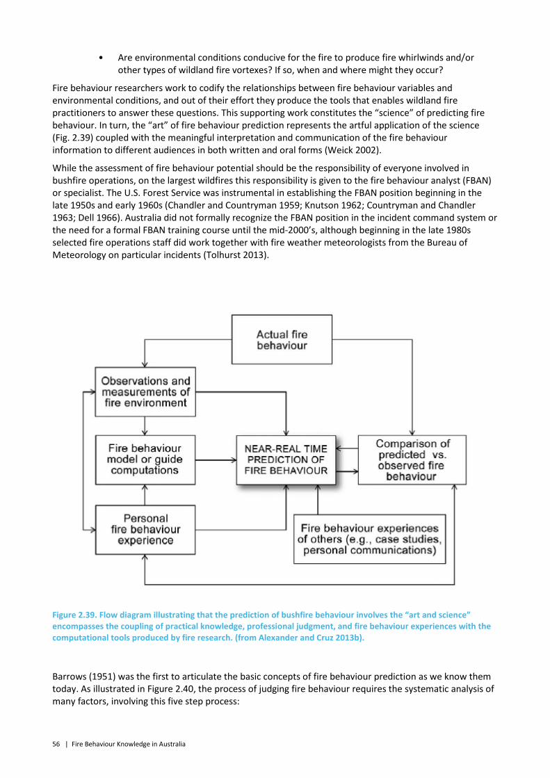
56 | Fire Behaviour Knowledge in Australia
• Are environmental conditions conducive for the fire to produce fire whirlwinds and/or other types of wildland fire vortexes? If so, when and where might they occur?
Fire behaviour researchers work to codify the relationships between fire behaviour variables and environmental conditions, and out of their effort they produce the tools that enables wildland fire practitioners to answer these questions. This supporting work constitutes the “science” of predicting fire behaviour. In turn, the “art” of fire behaviour prediction represents the artful application of the science (Fig. 2.39) coupled with the meaningful interpretation and communication of the fire behaviour information to different audiences in both written and oral forms (Weick 2002).
While the assessment of fire behaviour potential should be the responsibility of everyone involved in bushfire operations, on the largest wildfires this responsibility is given to the fire behaviour analyst (FBAN) or specialist. The U.S. Forest Service was instrumental in establishing the FBAN position beginning in the late 1950s and early 1960s (Chandler and Countryman 1959; Knutson 1962; Countryman and Chandler 1963; Dell 1966). Australia did not formally recognize the FBAN position in the incident command system or the need for a formal FBAN training course until the mid-2000’s, although beginning in the late 1980s selected fire operations staff did work together with fire weather meteorologists from the Bureau of Meteorology on particular incidents (Tolhurst 2013).
Figure 2.39. Flow diagram illustrating that the prediction of bushfire behaviour involves the “art and science” encompasses the coupling of practical knowledge, professional judgment, and fire behaviour experiences with the computational tools produced by fire research. (from Alexander and Cruz 2013b).
Barrows (1951) was the first to articulate the basic concepts of fire behaviour prediction as we know them today. As illustrated in Figure 2.40, the process of judging fire behaviour requires the systematic analysis of many factors, involving this five step process:
Fire Behaviour Knowledge in Australia | 57
Step 1: Basic knowledge. The foundation for judging probable fire behaviour must rest on basic knowledge of the principles of combustion: What is necessary for combustion to occur? What causes the rate of combustion to increase or decrease? How may combustion be reduced or stopped?
Step 2: Forest knowledge. Three basic factors in a forest area—weather, topography, and fuels—are important indicators of fire behaviour.
Step 3: Aids and guides. Several aids and guides are available to assist in evaluating weather, topography, and fuels.
Step 4: Estimate of situation. The probabilities for various patterns of fire behaviour are systematically explored through an estimate of the situation based upon the combined effects of weather, fuels, and topography.
Step 5: Decision. The end product of the fire behaviour analysis is a decision outlining when, where, and how to control the fire and spelling out any special safety measures required.
Figure 2.40. Predicting or forecasting fire behaviour requires the systematic analysis of many factors (from Barrows 1951).
These guidelines are applicable to both the control and use of planned or unplanned ignitions in bushfire management. They are also valid in the designing of simulation studies involving the prediction of free-spreading fire behaviour.
Bushfire behaviour predictions involve three sets of assumptions which in turn become the primary limitations in accurately predicting a fire’s behaviour. The first set of assumptions includes the general simplifying assumptions associated with any kind of the models or guides used for operationally predicting fire behaviour (e.g. Taylor et al. 1997; Gould et al. 2008; Pearce et al. 2012):
• The model or guide is applicable to the fuel conditions.
• The fuels are uniform and continuous.
58 | Fire Behaviour Knowledge in Australia
• The fuel moisture values used are representative of the fire site.
• The topography is simple and homogeneous.
• Wind speed is constant and unidirectional.
• The fire is free-burning and unaffected by fire suppression activities.
The second set of assumptions are those that underlie the specific model or guide in question. See, for example, the list of assumptions listed by Rothermel (1991, p 36-37) in his guide to predicting crown fire behaviour in conifer forests of the USA Northern Rocky Mountains. Ideally, this set of assumptions should include as a minimum the technical basis for the model or guide development (e.g., experimental fires and/or wildfire observations) and the range in environmental conditions and fire behaviour upon which they are considered valid for.
The third and final set of assumptions are those specified by the FBAN assigned to produce a forecast of fire behaviour for an actual wildfire incident. This would typically involve such items as the (i) date/time of fire perimeter assessment, known or assumed, used to project from, (ii) the date and time interval that the fire behaviour forecast is deemed valid for, (iii) the weather and topographic conditions applied to the situation at hand and their basis (e.g., from the fire weather forecast, local knowledge), and (iv) the model or guide used and why (including the fuel type or model selected) and any adjustment made to the outputs and the rationale for doing so.
Models and modelling are an integral component of modern day fire management practices (Alexander 2009). Models and guides used for predicting fire behaviour should obviously be sensitive to those parameters known to affect fire behaviour, namely variations in live and dead fuel moistures, wind speed, and slope steepness, amongst other factors, for a given fuel complex. All fire behaviour prediction tools will produce results which do not always agree exactly with observed fire behaviour. As Cheney (1981) points out:
The reality of fire behaviour predictions is that overestimates can be easily readjusted without serious consequences; underestimates of behaviour can be disastrous both to the operations of the fire controller and the credibility of the person making the predictions.
It is important that all fire practitioners realise that operational models and guides for predicting fire behaviour are mechanical in nature and in all likelihood will not produce an exact answer; Cruz and Alexander (2013) have shown how rate of fire spread can vary predicted and actual outcomes. As Albini (1976) has pointed out, there are three principal reasons for disagreement between model predictions and observed fire behaviour, no matter which models are being used (see Alexander and Cruz 2013b for further discussion):
• The model may not be applicable to the situation.
• The model’s inherent accuracy may be at fault.
• The data used in the model may be inaccurate.
With respect to the last category, error can unknowingly be introduced into a prediction as a result, for example, of a lack adherence to standards for fire weather stations (Cruz and Plucinski 2007) or unrealistic fuel type mapping.
On actual wildfire incidents, fire behaviour prediction accuracy is highly dependent upon the skill, knowledge, and experience of the practitioner (e.g., FBAN). To be truly good at predicting fire behaviour, as mentioned earlier, requires applying both the art and science to the task.
Burrows (1984) observed that most fire operations personnel base their expectations of how a fire will behave largely on experience and, to a lesser extent, on fire behaviour guides. Fire behaviour case study knowledge, coupled with experienced judgment and calculations made using fire behaviour models or guides, is generally considered as the most effective means of predicting fire behaviour. Experienced judgement is certainly needed in any prediction of fire behaviour but it does have its limitations. In this
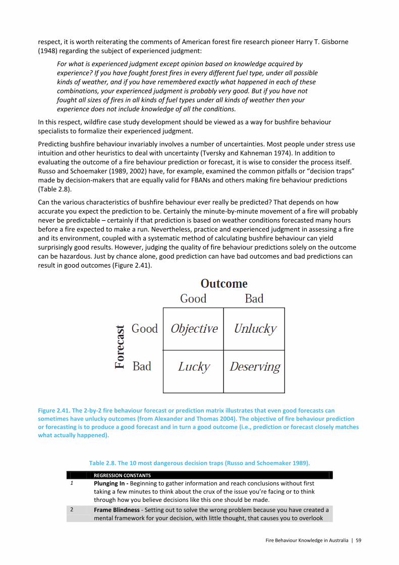
Fire Behaviour Knowledge in Australia | 59
respect, it is worth reiterating the comments of American forest fire research pioneer Harry T. Gisborne (1948) regarding the subject of experienced judgment:
For what is experienced judgment except opinion based on knowledge acquired by experience? If you have fought forest fires in every different fuel type, under all possible kinds of weather, and if you have remembered exactly what happened in each of these combinations, your experienced judgment is probably very good. But if you have not fought all sizes of fires in all kinds of fuel types under all kinds of weather then your experience does not include knowledge of all the conditions.
In this respect, wildfire case study development should be viewed as a way for bushfire behaviour specialists to formalize their experienced judgment.
Predicting bushfire behaviour invariably involves a number of uncertainties. Most people under stress use intuition and other heuristics to deal with uncertainty (Tversky and Kahneman 1974). In addition to evaluating the outcome of a fire behaviour prediction or forecast, it is wise to consider the process itself. Russo and Schoemaker (1989, 2002) have, for example, examined the common pitfalls or “decision traps” made by decision-makers that are equally valid for FBANs and others making fire behaviour predictions (Table 2.8).
Can the various characteristics of bushfire behaviour ever really be predicted? That depends on how accurate you expect the prediction to be. Certainly the minute-by-minute movement of a fire will probably never be predictable – certainly if that prediction is based on weather conditions forecasted many hours before a fire expected to make a run. Nevertheless, practice and experienced judgment in assessing a fire and its environment, coupled with a systematic method of calculating bushfire behaviour can yield surprisingly good results. However, judging the quality of fire behaviour predictions solely on the outcome can be hazardous. Just by chance alone, good prediction can have bad outcomes and bad predictions can result in good outcomes (Figure 2.41).
Figure 2.41. The 2-by-2 fire behaviour forecast or prediction matrix illustrates that even good forecasts can sometimes have unlucky outcomes (from Alexander and Thomas 2004). The objective of fire behaviour prediction or forecasting is to produce a good forecast and in turn a good outcome (i.e., prediction or forecast closely matches what actually happened).
Table 2.8. The 10 most dangerous decision traps (Russo and Schoemaker 1989).
REGRESSION CONSTANTS 1 Plunging In - Beginning to gather information and reach conclusions without first
taking a few minutes to think about the crux of the issue you’re facing or to think through how you believe decisions like this one should be made.
2 Frame Blindness - Setting out to solve the wrong problem because you have created a mental framework for your decision, with little thought, that causes you to overlook
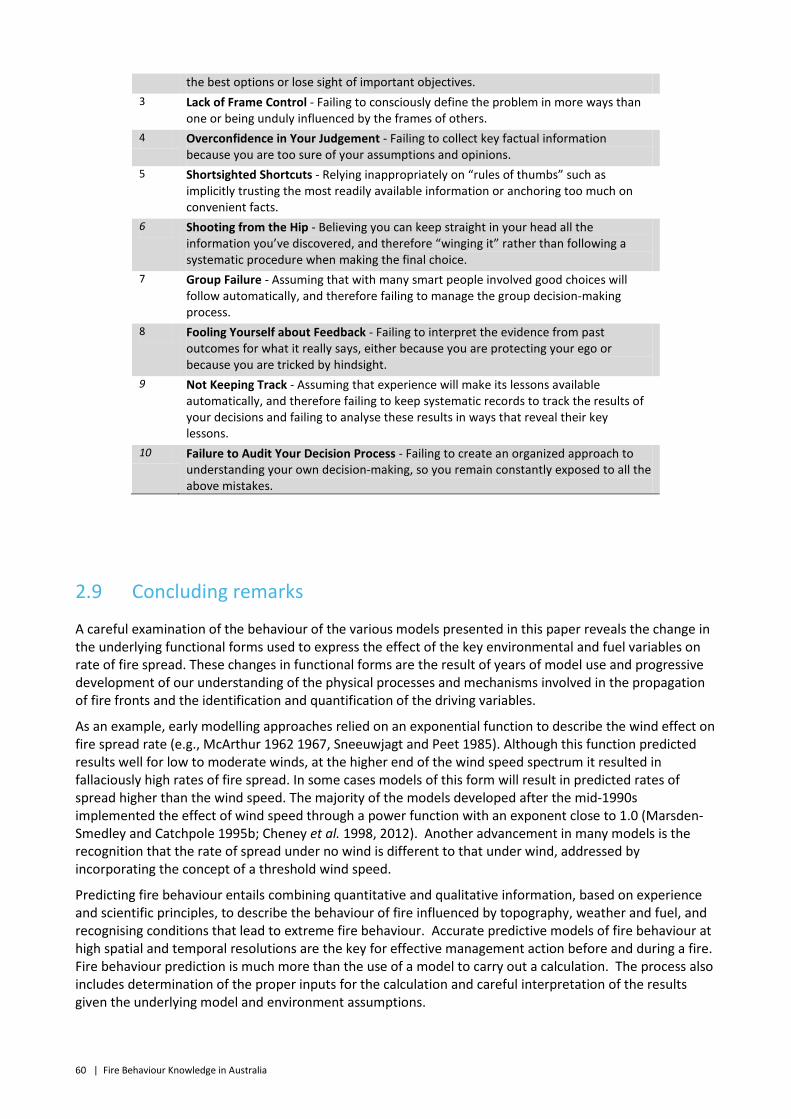
60 | Fire Behaviour Knowledge in Australia
the best options or lose sight of important objectives. 3 Lack of Frame Control - Failing to consciously define the problem in more ways than
one or being unduly influenced by the frames of others. 4 Overconfidence in Your Judgement - Failing to collect key factual information
because you are too sure of your assumptions and opinions. 5 Shortsighted Shortcuts - Relying inappropriately on “rules of thumbs” such as
implicitly trusting the most readily available information or anchoring too much on convenient facts.
6 Shooting from the Hip - Believing you can keep straight in your head all the information you’ve discovered, and therefore “winging it” rather than following a systematic procedure when making the final choice.
7 Group Failure - Assuming that with many smart people involved good choices will follow automatically, and therefore failing to manage the group decision-making process.
8 Fooling Yourself about Feedback - Failing to interpret the evidence from past outcomes for what it really says, either because you are protecting your ego or because you are tricked by hindsight.
9 Not Keeping Track - Assuming that experience will make its lessons available automatically, and therefore failing to keep systematic records to track the results of your decisions and failing to analyse these results in ways that reveal their key lessons.
10 Failure to Audit Your Decision Process - Failing to create an organized approach to understanding your own decision-making, so you remain constantly exposed to all the above mistakes.
2.9 Concluding remarks
A careful examination of the behaviour of the various models presented in this paper reveals the change in the underlying functional forms used to express the effect of the key environmental and fuel variables on rate of fire spread. These changes in functional forms are the result of years of model use and progressive development of our understanding of the physical processes and mechanisms involved in the propagation of fire fronts and the identification and quantification of the driving variables.
As an example, early modelling approaches relied on an exponential function to describe the wind effect on fire spread rate (e.g., McArthur 1962 1967, Sneeuwjagt and Peet 1985). Although this function predicted results well for low to moderate winds, at the higher end of the wind speed spectrum it resulted in fallaciously high rates of fire spread. In some cases models of this form will result in predicted rates of spread higher than the wind speed. The majority of the models developed after the mid-1990s implemented the effect of wind speed through a power function with an exponent close to 1.0 (Marsden-Smedley and Catchpole 1995b; Cheney et al. 1998, 2012). Another advancement in many models is the recognition that the rate of spread under no wind is different to that under wind, addressed by incorporating the concept of a threshold wind speed.
Predicting fire behaviour entails combining quantitative and qualitative information, based on experience and scientific principles, to describe the behaviour of fire influenced by topography, weather and fuel, and recognising conditions that lead to extreme fire behaviour. Accurate predictive models of fire behaviour at high spatial and temporal resolutions are the key for effective management action before and during a fire. Fire behaviour prediction is much more than the use of a model to carry out a calculation. The process also includes determination of the proper inputs for the calculation and careful interpretation of the results given the underlying model and environment assumptions.
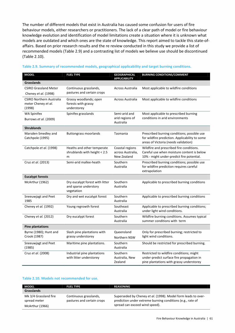
Fire Behaviour Knowledge in Australia | 61
The number of different models that exist in Australia has caused some confusion for users of fire behaviour models, either researchers or practitioners. The lack of a clear path of model or fire behaviour knowledge evolution and identification of model limitations create a situation where it is unknown what models are outdated and which ones are the state of knowledge. This report aimed to tackle this state-of-affairs. Based on prior research results and the re review conducted in this study we provide a list of recommended models (Table 2.9) and a contrasting list of models we believe use should be discontinued (Table 2.10).
Table 2.9. Summary of recommended models, geographical applicability and target burning conditions.
MODEL FUEL TYPE GEOGRAPHICAL APPLICABILITY
BURNING CONDITIONS/COMMENT
Grasslands CSIRO Grassland Meter Cheney et al. (1998)
Continuous grasslands, pastures and certain crops
Across Australia Most applicable to wildfire conditions
CSIRO Northern Australia meter Cheney et al. (1998)
Grassy woodlands; open forests with grassy understorey
Across Australia Most applicable to wildfire conditions
WA Spinifex Burrows et al. (2009)
Spinifex grasslands Semi-arid and arid regions of Australia
Most applicable to prescribed burning conditions in arid environments
Shrublands Marsden-Smedley and Catchpole (1995)
Buttongrass moorlands Tasmania Prescribed burning conditions; possible use for wildfire prediction. Applicability to some areas of Victoria (needs validation)
Catchpole et al. (1998) Heaths and other temperate shrublands with height < 2.5 m
Coastal regions across Australia, New Zealand
Wildfire and prescribed fire conditions. Careful use when moisture content is below 10% - might under-predict fire potential.
Cruz et al. (2013) Semi-arid mallee-heath Southern Australia
Prescribed burning conditions; possible use for wildfire prediction requires careful extrapolation
Eucalypt forests McArthur (1962) Dry eucalypt forest with litter
and sparse understory vegetation
Southern Australia
Applicable to prescribed burning conditions
Sneeuwjagt and Peet 1985
Dry and wet eucalypt forest Southern Australia
Applicable to prescribed burning conditions
Cheney et al. (1992) Young regrowth forest Southeast Australia
Applicable to prescribed burning conditions; under light wind conditions.
Cheney et al. (2012) Dry eucalypt forest Southern Australia
Wildfire burning conditions. Assumes typical summer conditions with term
Pine plantations Byrne (1980); Hunt and Crook (1987)
Slash pine plantations with grassy understorey
Queensland Northern NSW
Only for prescribed burning; restricted to light wind conditions.
Sneeuwjagt and Peet (1985)
Maritime pine plantations. Southern Australia
Should be restricted for prescribed burning.
Cruz et al. (2008) Industrial pine plantations with litter understorey
Southern Australia, New Zealand
Restricted to wildfire conditions; might under-predict surface fire propagation in pine plantations with grassy understorey
Table 2.10. Models not recommended for use.
MODEL FUEL TYPE REASONING Grasslands Mk 3/4 Grassland fire spread meter McArthur (1966)
Continuous grasslands, pastures and certain crops
Superseded by Cheney et al. (1998). Model form leads to over-prediction under extreme burning conditions (e.g., rate of spread can exceed wind speed).
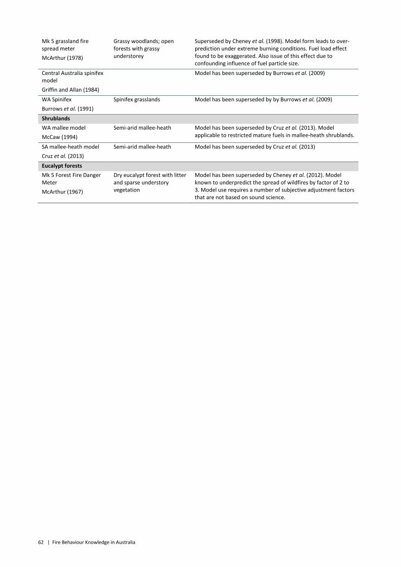
62 | Fire Behaviour Knowledge in Australia
Mk 5 grassland fire spread meter McArthur (1978)
Grassy woodlands; open forests with grassy understorey
Superseded by Cheney et al. (1998). Model form leads to over-prediction under extreme burning conditions. Fuel load effect found to be exaggerated. Also issue of this effect due to confounding influence of fuel particle size.
Central Australia spinifex model Griffin and Allan (1984)
Model has been superseded by Burrows et al. (2009)
WA Spinifex Burrows et al. (1991)
Spinifex grasslands Model has been superseded by by Burrows et al. (2009)
Shrublands WA mallee model McCaw (1994)
Semi-arid mallee-heath Model has been superseded by Cruz et al. (2013). Model applicable to restricted mature fuels in mallee-heath shrublands.
SA mallee-heath model Cruz et al. (2013)
Semi-arid mallee-heath Model has been superseded by Cruz et al. (2013)
Eucalypt forests Mk 5 Forest Fire Danger Meter McArthur (1967)
Dry eucalypt forest with litter and sparse understory vegetation
Model has been superseded by Cheney et al. (2012). Model known to underpredict the spread of wildfires by factor of 2 to 3. Model use requires a number of subjective adjustment factors that are not based on sound science.
Fire Behaviour Knowledge in Australia | 63
3 Fire Perimeter Propagation Modelling
3.1 Introduction
The preceding chapter focused solely on the discussion of the development and published evaluations of rate of fire spread models in Australian vegetation types. These models are all specifically designed to provide an estimate of the speed of movement of the head fire (defined as the part of a fire perimeter where the rate of spread, flame height and intensity are greatest, usually when burning downwind or upslope (AFAC 2012)) in a particular fuel type under a finite range of conditions. As a result of their generally analytical nature (e.g. consisting often of a single mathematical relation that has a closed form solution), the level of technical sophistication required to implement these models is generally quite low. These have taken the form of tables, circular and linear slide rules, or even simple rules of thumb.
However, in order to simulate the spread of a whole fire perimeter, additional information is needed about the rate of expansion of the perimeter in directions other than that of the head fire.
A number of methods have been developed over the years to simulate the propagation of the entire fire perimeter. These range from crude approximations of rate of area and perimeter increase based on rate of forward spread, geometric approximations based on given fire perimeter shapes, through to fully physical models of flame propagation in three dimensions.
In these models, the primary output is an estimate of the propagation, or progression, of a fire perimeter across a landscape. Often this is in the form of a map of fire perimeter isochrones or time of arrival of the fire perimeter at given locations.
The task of carrying out the calculations for perimeter propagation can be done manually and, indeed, has been done this way for many years--applying the selected rate of forward spread models as needed, correcting for topographic effects as required, applying the selected perimeter expansion method and drawing a map of the expected progress of the fire by hand. However, in recent years a number of computer applications have been constructed to make the task simpler and faster.
This chapter provides a brief overview of the range of computerised methodologies that have been developed and then provides more detail on the much reduced number of automated fire spread simulation packages currently employed in Australasia.
3.2 Fire perimeter propagation methodologies
Fire behaviour models may be divided into three broad categories (Sullivan 2009a, b, c). These are: physical and quasi-physical models; empirical and quasi-empirical models; and simulation or mathematical analogue models, depending on whether they attempt represent the underlying fundamental physics or chemistry of fire spread, contain little or no physical basis (generally only statistical in nature), or utilise a mathematical precept rather than a physical one for the modelling of the spread of wildland fire.
Similarly, fire perimeter propagation methods may be divided into two broad categories, based on the complexity of the approach. As would be expected, these are related to the categories of fire behaviour models. They are:
1.Computational fluid dynamic (CFD) models, and
2.Simulation models.
Computational fluid dynamic (CFD) models are similar to physical fire behaviour models in that they attempt to replicate fire behaviour based on the fundamental combustion chemistry and heat transfer physics but are more strictly limited to those that do so in a full three-dimensional framework. Lower

64 | Fire Behaviour Knowledge in Australia
dimensional physical models do exist (2D and even 1D) but these do not generally provide a map of the propagation of the entire perimeter.
CFD models are based on the compressible Navier Stokes equations for the motion of fluids, with associated auxiliary relationships for factors such as chemical reactions and turbulence. Such models are less reliant upon extensive experimental relations for robustness, but are very computationally expensive and can currently still only model a fraction of the complex processes occurring within wildfires.
Simulation models are essentially the empirical fire behaviour model equivalent in that they generally do not incorporate any physical considerations but apply empirical rate of spread models to simulate the propagation of the fire perimeter in an attempt to model the large-scale propagation of fire across a landscape. As such, they can be based on simplified versions of more complex physical (CFD) models, use empirical relationships measured in the field, or be based on an unrelated mathematical rule set. Generally they require additional model components to convert the essentially one dimensional empirical rate of spread model to one that can propagate an entire perimeter
3.3 Computational fluid dynamic modelling
Wildland fire is the complicated combination of energy released (in the form of heat) due to chemical reactions (broadly categorised as an oxidation reaction) in the process of combustion and the transport of that energy to surrounding unburnt fuel and the subsequent ignition of said fuel. The former is the domain of chemistry (more specifically, chemical kinetics) and occurs on the scale of molecules and nano-seconds, and the latter is the domain of physics (more specifically, heat transfer and fluid mechanics) and occurs on scales ranging from millimetres up to kilometres, seconds up to hours.
It is the interaction of these processes over the wide range of temporal and spatial scales that makes the modelling of wildland fire behaviour a challenging task.
Grishin (1997, pg. 81) proposed five relative independent stages in the development of a deterministic physical model of wildland fire behaviour:
1. Physical analysis of the phenomenon of wildland fire spread; isolation of the mechanism governing the transfer of energy from the fire front into the environment; definition of the medium type, and creation of a physical model of the phenomenon.
2. Determination of the reaction and thermophysical properties of the medium, the transfer coefficients and structural parameters of the medium, and deduction of the basic system of equations with corresponding additional (boundary and initial) conditions.
3. Selection of a method of numerical solution of the problem, and derivation of differential equations approximating the basic system of equations.
4. Programming; test check of the program; evaluation of the accuracy of the difference scheme; numerical solution of the system of equations.
5. Testing to see how well the derived results comply with the real system; their physical interpretation; development of new technical suggestions for ways of fighting wildland fire.
Clearly, stages one and two represent considerable hurdles and sources of contention for the best method in which to represent the phenomenon of wildland fire.
3.3.1 CHEMISTRY OF COMBUSTION
The chemistry of combustion involved in wildland fire is necessarily a complex and complicated matter. This is in part due to the complicated nature of the fuel itself but also in the range of conditions over which combustion processes occur (Sullivan and Ball 2012). The chemistry of combustion includes:
• Fuel chemistry (the chemical make-up of the fuel itself, predominantly incorporating sugar-based polymers)
Fire Behaviour Knowledge in Australia | 65
• Thermal degradation reactions (the initial thermal scission of fuel polymers under heating, pyrolysis and charring)
• Gas-phase reactions (flaming combustion of volatile products) • Solid-phase reactions (glowing combustion of charring products)
The heat released from these reactions is then transferred to adjacent unburnt fuel which can then ignite and propagate the fire. The mechanisms by which this heat is transferred is in the domain of the physics of combustion.
3.3.2 PHYSICS OF COMBUSTION AND FIRE SPREAD
The physics involved in the combustion of wildland fuel and the behaviour of wildland fires is, like the chemistry, complicated and highly dependent on the conditions in which a fire is burning. Williams (1982) gives nine possible mechanisms for the transfer of heat from a fire:
1. Diffusion of radicals
2. Heat conduction through a gas
3. Heat conduction through condensed materials
4. Convection through a gas
5. Liquid convection
6. Fuel deformation
7. Radiation from flames
8. Radiation from burning fuel surfaces
9. Firebrand transport.
1, 2 and 3 could be classed as diffusion at the molecular level. 4 and 5 are convection (although the presence of liquid phase fuel is extremely rare) but can be generalised to advection to include any transfer of heat through the motion of gases. 7 and 8 are radiation. 6 and 9 could be classed as solid fuel transport. This roughly translates to the three generally accepted forms of heat transfer (conduction, convection and radiation) plus solid fuel transport, which, as Emmons (1966) points out, is not trivial or unimportant in wildland fires.
The primary physical processes driving the transfer of heat in a wildland fire are that of advection and radiation. In low wind conditions, the dominating process is that of radiation (Weber 1989). In conditions where wind is not insignificant, it is advection that dominates (Grishin 1984). However, it is not reasonable to assume one works without the other and thus both mechanisms must be considered.
In attempting to represent the role of advection in wildland fire spread, the application of fluid dynamics is of prime importance. This assumes that the gas flow can be considered as a continuous medium or fluid.
Advection or Fluid transport
Fluid dynamics is a large area of active research and the basic outlines of the principles are given here. The interested reader is directed to a considerable number of texts on the subject for more in-depth discussion (e.g. Batchelor (1967); Turner (1973)).
The key aspect of fluid dynamics and its application to understanding the motion of gases is the notion of continuity. Here, the molecules or particles of a gas are considered to be continuous and thus behave as a fluid rather than a collection of particles. Another key aspect of fluid mechanics (and physics in general) is the fundamental notion of the conservation of quantities which is encompassed in the fluidised equations of motion.
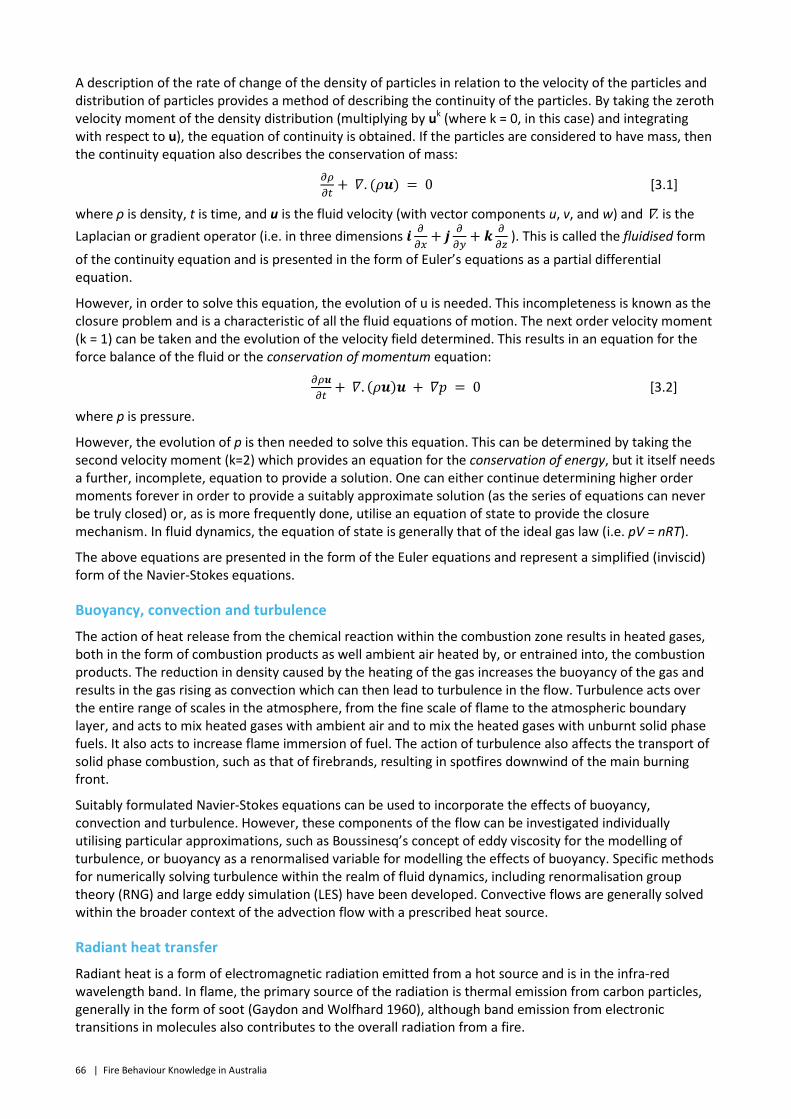
66 | Fire Behaviour Knowledge in Australia
A description of the rate of change of the density of particles in relation to the velocity of the particles and distribution of particles provides a method of describing the continuity of the particles. By taking the zeroth velocity moment of the density distribution (multiplying by uk (where k = 0, in this case) and integrating with respect to u), the equation of continuity is obtained. If the particles are considered to have mass, then the continuity equation also describes the conservation of mass:
𝜕𝜌𝜕𝑡
+ 𝛻. (𝜌𝒖) = 0 [3.1]
where ρ is density, t is time, and u is the fluid velocity (with vector components u, v, and w) and ∇. is the Laplacian or gradient operator (i.e. in three dimensions 𝒊 𝜕
𝜕𝑥+ 𝒋 𝜕
𝜕𝑦+ 𝒌 𝜕
𝜕𝑧 ). This is called the fluidised form
of the continuity equation and is presented in the form of Euler’s equations as a partial differential equation.
However, in order to solve this equation, the evolution of u is needed. This incompleteness is known as the closure problem and is a characteristic of all the fluid equations of motion. The next order velocity moment (k = 1) can be taken and the evolution of the velocity field determined. This results in an equation for the force balance of the fluid or the conservation of momentum equation:
𝜕𝜌𝒖𝜕𝑡
+ 𝛻. (𝜌𝒖)𝒖 + 𝛻𝑝 = 0 [3.2]
where p is pressure.
However, the evolution of p is then needed to solve this equation. This can be determined by taking the second velocity moment (k=2) which provides an equation for the conservation of energy, but it itself needs a further, incomplete, equation to provide a solution. One can either continue determining higher order moments forever in order to provide a suitably approximate solution (as the series of equations can never be truly closed) or, as is more frequently done, utilise an equation of state to provide the closure mechanism. In fluid dynamics, the equation of state is generally that of the ideal gas law (i.e. pV = nRT).
The above equations are presented in the form of the Euler equations and represent a simplified (inviscid) form of the Navier-Stokes equations.
Buoyancy, convection and turbulence
The action of heat release from the chemical reaction within the combustion zone results in heated gases, both in the form of combustion products as well ambient air heated by, or entrained into, the combustion products. The reduction in density caused by the heating of the gas increases the buoyancy of the gas and results in the gas rising as convection which can then lead to turbulence in the flow. Turbulence acts over the entire range of scales in the atmosphere, from the fine scale of flame to the atmospheric boundary layer, and acts to mix heated gases with ambient air and to mix the heated gases with unburnt solid phase fuels. It also acts to increase flame immersion of fuel. The action of turbulence also affects the transport of solid phase combustion, such as that of firebrands, resulting in spotfires downwind of the main burning front.
Suitably formulated Navier-Stokes equations can be used to incorporate the effects of buoyancy, convection and turbulence. However, these components of the flow can be investigated individually utilising particular approximations, such as Boussinesq’s concept of eddy viscosity for the modelling of turbulence, or buoyancy as a renormalised variable for modelling the effects of buoyancy. Specific methods for numerically solving turbulence within the realm of fluid dynamics, including renormalisation group theory (RNG) and large eddy simulation (LES) have been developed. Convective flows are generally solved within the broader context of the advection flow with a prescribed heat source.
Radiant heat transfer
Radiant heat is a form of electromagnetic radiation emitted from a hot source and is in the infra-red wavelength band. In flame, the primary source of the radiation is thermal emission from carbon particles, generally in the form of soot (Gaydon and Wolfhard 1960), although band emission from electronic transitions in molecules also contributes to the overall radiation from a fire.

Fire Behaviour Knowledge in Australia | 67
The general method of modelling radiant heat transfer is through the use of a radiant transfer equation (RTE) of which the simplest is that of the Stefan-Boltzmann equation:
𝑞 = 𝜎𝑇4 [3.3]
where σ is the Stefan-Boltzmann constant (5.67 × 10⁻⁸ JK−4 m−2 s−1 and T is the radiating temperature of the surface (K).
While it is possible to approximate the radiant heat flux from a fire as a surface emission from the flame face, this does not fully capture the volumetric emission nature of the flame (Sullivan et al. 2003) and can lead to inaccuracies in flux estimations if precise flame geometry (i.e. view factor), temperature and emissivity equivalents are not known.
More complex solutions of the RTE, such as treating the flame as a volume of radiation emitting, scattering and absorbing media, can improve the prediction of radiant heat but are necessarily more computationally intensive; varying levels of approximation (both physical and numerical) are frequently employed to improve the computational efficiency.
The Discrete Transfer Radiation Model (DTRM) solves the radiative transfer equation throughout a domain by a method of ray tracing from surface elements on its boundaries and thus does not require information about the radiating volume itself. Discrete Ordinate Method (DOM) divides the volume into discrete volumes for which the full RTE is solved at each instance and the sum of radiation along all paths from an observer calculated. The Differential Approximation (or P1 method) solves the RTE as a diffusion equation which includes the effect of scattering but assumes the media is optically thick. Knowledge about the media’s absorption, scattering, refractive index, path length and local temperature are required for many of these solutions. Descriptions of methods for solving these forms of the RTE are given in texts on radiant heat transfer (e.g. Drysdale (1985)). Sacadura (2005) and Goldstein et al. (2006) review the use of radiative heat transfer models in a wide range of applications.
Transmission of thermal radiation can be affected by smoke or band absorption by certain components of the atmosphere (e.g. CO2 , H2O).
Firebrands (solid fuel transport)
Determination of the transport of solid fuel (i.e. firebrands), which leads to the initiation of spotfires downwind of the main fire front is highly probabilistic (Ellis 2000, 2011, 2013) and not readily amenable to a purely deterministic description. This is due in part to the wide variation in firebrand sources and ignitions and the particular flight paths any firebrand might take. Maximum distance that a firebrand may be carried is determined by the intensity of the fire and the updraught velocity of the convection, the height at which the firebrand was sourced and the wind profile aloft (Albini 1979; Ellis 2000, Albini et al. 2012). Whether or not the firebrand lands alight and starts a spotfire is dependent upon the nature of the firebrand, how it was ignited, its combustion properties (including flaming lifetime) and the ignition properties of the fuel in which it lands (e.g. moisture content, bulk density, etc) (Plucinski and Anderson 2008; Sullivan et al. 2013).
Atmospheric interactions
The transport of the gas phase of the combustion products interacts with the atmosphere around it, transferring heat and energy, through convection and turbulence. The condition of the atmosphere, particularly the lapse rate, or the ease with which heated parcels of air rise within the atmosphere, controls the impact that buoyancy of the heated air from the combustion zone has on the atmosphere and the fire.
Changes in the ambient meteorological conditions, such as changes in wind speed and direction, moisture, temperature, lapse rates, etc, both at the surface and higher in the atmosphere, can have a significant impact on the state of the fuel (moisture content), the behaviour of a fire, its growth, and, in turn, the impact that fire can have on the atmosphere itself.

68 | Fire Behaviour Knowledge in Australia
Topographic interactions
The topography in which a fire is burning also plays a part in the way in which energy is transferred to unburnt fuel and the ambient atmosphere. It has long been recognised that fires burn faster upslope than they do down, even with a downslope wind. This is thought to be due to increased transfer of radiant heat due to the change in the geometry between the fuel on the slope and the flame, however recent work by Wu et al. (2000) suggests that there is also increased advection in these cases.
3.4 Computational fluid dynamics models
This section briefly describes three of the more complete physical and quasi-physical CFD models of fire perimeter propagation that have achieved a level of utilisation within the international bushfire research community (none of these models has yet to achieve consistent utilisation within the operational bushfire community). All are based on much the same basic principles as described in the preceding section and differ only in the methodology of implementation (choice of numerical solver, method of discretisation, selection of sub (e.g. turbulence) models).
They are presented in chronological order of first publication. While all have continued development since first publication, the rate of development differs markedly amongst the models. Some have been implemented and tested against observations, others have not. Where information about the performance of the model on available computing hardware is available in the literature, this is presented.
Generally, the primary output of these CFD models is a significant amount of data for a large number of variables within a three-dimensional mesh (the simulation domain)—essentially a large text file filled with numbers. These variables may include gas temperature, species concentration, velocity, pressure, etc. In order for the results to be readily discerned by a human, they must first be processed or rendered into a graphical form—either a static picture of the output at a given time or a video of the output as it evolves over time. This post-processing of the simulation output can range from the simple colouring of vectors, which may take a relatively short time (minutes to hours), to a fully rendered photo-realistic 3D image of a scene that may take a very long time (hours to days). The quality of the rendered output does not necessarily reflect the quality of the simulation; many people may be impressed by a realistically coloured image but it may not be very helpful.
3.4.1 FIRETEC (LOS ALAMOS NATIONAL LABORATORY, USA)
FIRETEC (Linn 1997), developed at the Los Alamos National Laboratory, USA, is a coupled multiphase transport/wildland fire model based on the principles of conservation of mass, momentum and energy. It is fully three-dimensional and in combination with a hydrodynamics model called HIGRAD (Reisner et al. 1998, 2000a,b), which is used to solve equations of high gradient flow such as the motions of the local atmosphere, it employs a fully compressible gas transport formulation to represent the coupled interactions of the combustion, heat transfer and fluid mechanics involved in wildland fire (Linn et al. 2002). Figure 3.1 and Figure 3.2 show different visualisations of the output of the model.
FIRETEC is described by the author as self-determining, by which it is meant that the model does not use prescribed or empirical relations in order to predict the spread and behaviour of wildland fires, relying solely on the formulations of the physics and chemistry to model the fire behaviour. The model utilises the finite volume method and the notion of a resolved volume to solve numerically its system of equations. It attempts to represent the average behaviour of the gases and solid fuels in the presence of a wildland fire.
Many small-scale processes such as convective heat transfer between solids and gases are represented without each process actually being resolved in detail (Linn 1997; Linn and Harlow 1998a). Fine scale wind patterns around structures smaller than the resolved scale of the model, including individual flames, are not represented explicitly.
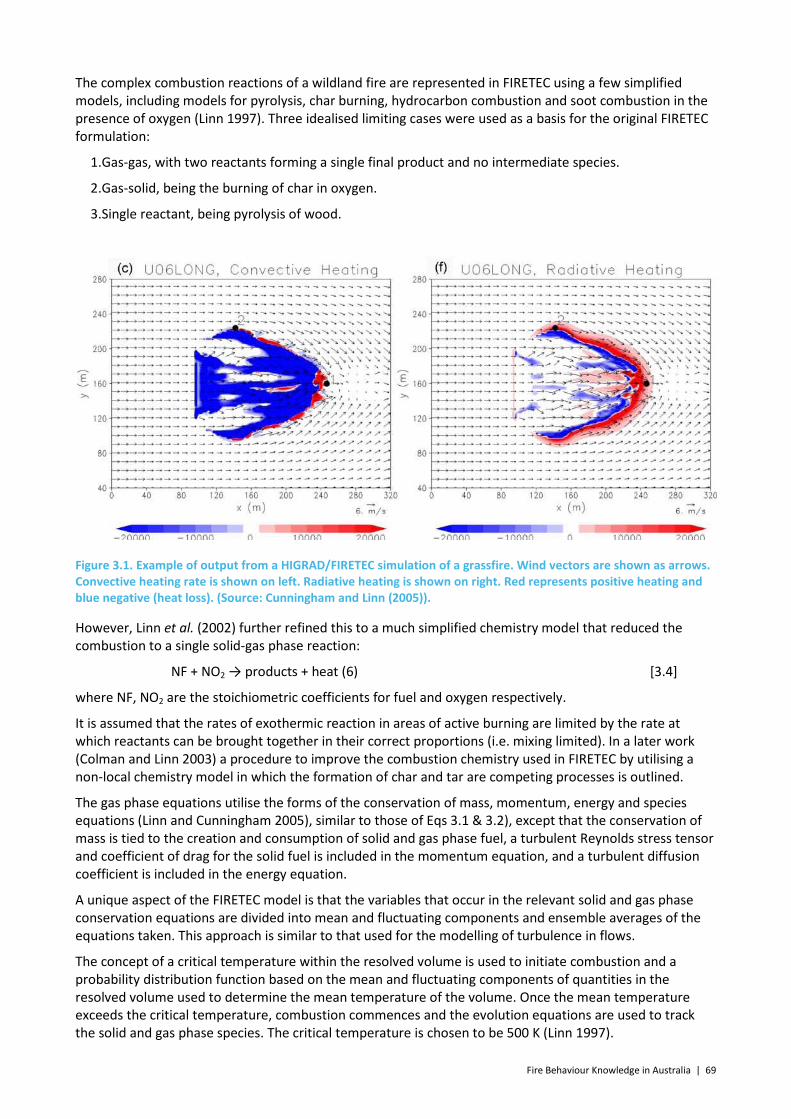
Fire Behaviour Knowledge in Australia | 69
The complex combustion reactions of a wildland fire are represented in FIRETEC using a few simplified models, including models for pyrolysis, char burning, hydrocarbon combustion and soot combustion in the presence of oxygen (Linn 1997). Three idealised limiting cases were used as a basis for the original FIRETEC formulation:
1.Gas-gas, with two reactants forming a single final product and no intermediate species.
2.Gas-solid, being the burning of char in oxygen.
3.Single reactant, being pyrolysis of wood.
Figure 3.1. Example of output from a HIGRAD/FIRETEC simulation of a grassfire. Wind vectors are shown as arrows. Convective heating rate is shown on left. Radiative heating is shown on right. Red represents positive heating and blue negative (heat loss). (Source: Cunningham and Linn (2005)).
However, Linn et al. (2002) further refined this to a much simplified chemistry model that reduced the combustion to a single solid-gas phase reaction:
NF + NO2 → products + heat (6) [3.4]
where NF, NO2 are the stoichiometric coefficients for fuel and oxygen respectively.
It is assumed that the rates of exothermic reaction in areas of active burning are limited by the rate at which reactants can be brought together in their correct proportions (i.e. mixing limited). In a later work (Colman and Linn 2003) a procedure to improve the combustion chemistry used in FIRETEC by utilising a non-local chemistry model in which the formation of char and tar are competing processes is outlined.
The gas phase equations utilise the forms of the conservation of mass, momentum, energy and species equations (Linn and Cunningham 2005), similar to those of Eqs 3.1 & 3.2), except that the conservation of mass is tied to the creation and consumption of solid and gas phase fuel, a turbulent Reynolds stress tensor and coefficient of drag for the solid fuel is included in the momentum equation, and a turbulent diffusion coefficient is included in the energy equation.
A unique aspect of the FIRETEC model is that the variables that occur in the relevant solid and gas phase conservation equations are divided into mean and fluctuating components and ensemble averages of the equations taken. This approach is similar to that used for the modelling of turbulence in flows.
The concept of a critical temperature within the resolved volume is used to initiate combustion and a probability distribution function based on the mean and fluctuating components of quantities in the resolved volume used to determine the mean temperature of the volume. Once the mean temperature exceeds the critical temperature, combustion commences and the evolution equations are used to track the solid and gas phase species. The critical temperature is chosen to be 500 K (Linn 1997).
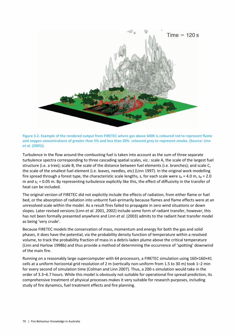
70 | Fire Behaviour Knowledge in Australia
Figure 3.2. Example of the rendered output from FIRETEC where gas above 600K is coloured red to represent flame and oxygen concentrations of greater than 5% and less than 20% coloured grey to represent smoke. (Source: Linn et al. (2005)).
Turbulence in the flow around the combusting fuel is taken into account as the sum of three separate turbulence spectra corresponding to three cascading spatial scales, viz.: scale A, the scale of the largest fuel structure (i.e. a tree); scale B, the scale of the distance between fuel elements (i.e. branches); and scale C, the scale of the smallest fuel element (i.e. leaves, needles, etc) (Linn 1997). In the original work modelling fire spread through a forest type, the characteristic scale lengths, s, for each scale were sA = 4.0 m, sB = 2.0 m and sC = 0.05 m. By representing turbulence explicitly like this, the effect of diffusivity in the transfer of heat can be included.
The original version of FIRETEC did not explicitly include the effects of radiation, from either flame or fuel bed, or the absorption of radiation into unburnt fuel–primarily because flames and flame effects were at an unresolved scale within the model. As a result fires failed to propagate in zero wind situations or down slopes. Later revised versions (Linn et al. 2001, 2002) include some form of radiant transfer, however, this has not been formally presented anywhere and Linn et al. (2003) admits to the radiant heat transfer model as being ‘very crude’.
Because FIRETEC models the conservation of mass, momentum and energy for both the gas and solid phases, it does have the potential, via the probability density function of temperature within a resolved volume, to track the probability fraction of mass in a debris-laden plume above the critical temperature (Linn and Harlow 1998b) and thus provide a method of determining the occurrence of ‘spotting’ downwind of the main fire.
Running on a reasonably large supercomputer with 64 processors, a FIRETEC simulation using 160×160×41 cells at a uniform horizontal grid resolution of 2 m (vertically non-uniform from 1.5 to 30 m) took 1–2 min for every second of simulation time (Colman and Linn 2007). Thus, a 200-s simulation would take in the order of 3.3–6.7 hours. While this model is obviously not suitable for operational fire spread prediction, its comprehensive treatment of physical processes makes it very suitable for research purposes, including study of fire dynamics, fuel treatment effects and fire planning.

Fire Behaviour Knowledge in Australia | 71
Figure 3.3. FIRETEC simulation (top) of an International Crown Fire Modelling Experiment fire in the Northwest Territories, Canada. (Source: http://www.scidacreview.org/0702/html/hardware.html).
According to the developer’s website, HIGRAD/FIRETEC is “currently being used to study the interaction between nonhomogeneities in vegetation, topography, and atmospheric conditions. Examples of the types of physical phenomenon of interest are the effects of transient wind conditions (i.e. gusts and meteorological changes), the effects of nonhomogeneous terrain (i.e. upslope canyons, saddles), and the effects of nonuniform fuels (i.e. patchy distributions), and influence of other disturbances on fire behavior (i.e. bark beetle attacks and fuels management tactics.)”
3.4.2 WFDS (NATIONAL INSTITUTE OF STANDARDS AND TECHNOLOGY, USA)
The Wildland Fire Dynamic Simulator (WFDS), developed initially by the US National Institute of Standards Technology (Mell et al. 2006) but more recently by the US Forest Service, is an extension of the model originally developed to predict the spread of fire within structures, the Fire Dynamic Simulator (FDS).
This model is fully 3D, is based upon a unique formulation of the equations of motion for buoyant flow (Rehm and Baum 1978) and is intended for use in predicting the behaviour of fires burning through peri-urban/wildlands (what the authors call ‘Community-scale fire spread’ (Rehm et al. 2003; Evans et al. 2003)). The main objective of this model is to predict the progress of fire through predominantly wildland fuel augmented by the presence of combustible structures.
WFDS utilises a varying computational grid to resolve volumes as low as 1.6 m (x) × 1.6 m (y) × 1.4 m (z) within a simulation domain in the order of 1.5 km2 in area and 200 m high. Outside regions of interest, the grid resolution is decreased to improve computation efficiency.
Mell et al. (2007) give a detailed description of the WFDS formulated for the specific initial case of grassland fuels (Figure 3.4), in which vegetation is not resolved in the gas-phase (atmosphere) grid but in a separate

72 | Fire Behaviour Knowledge in Australia
solid fuel (surface) grid (which the authors admit is not suitable for fuels in which there is significant vertical flame spread and air flow through the fuel). In the case presented, the model includes features such as momentum drag caused by the presence of the grass fuel (modelled as cylinders) which changes over time as the fuel is consumed. Mechanical turbulence, through the dynamic viscosity of the flow through the fuel, is modelled as a sub-grid parameter via a variant of the Large Eddy Simulation (LES) method.
Figure 3.4. Example of rendered output from WFDS where a CSIRO grassfire experiment was simulated. Flames are represented as orange, smoke as black. (Source: Mell et al. 2007).
The WFDS assumes a two-stage endothermic thermal decomposition (water evaporation and then solid fuel ‘pyrolysis’). It uses the temperature dependent mass loss rate expression of Morvan and Dupuy (2004) to model the solid fuel degradation and assumes that pyrolysis occurs at 127°C. Solid fuel is represented as a series of layers which are consumed from the top down until the solid mass reaches a predetermined char fraction at which point the fuel is considered consumed.
WFDS assumes combustion occurs solely as the result of fuel gas and oxygen mixing in stoichiometric proportion (and thus is independent of temperature). Char oxidation is not accounted for. The gas phase combustion is modelled using the following stoichiometric relation:
C3.4H6.2O2.5 + 3.7(O2 + 3.76N2) → 3.4CO2 + 3.1H2O + 13.91N2 [3.5]
Due to the relatively coarse scale of the resolved computation grids within WFDS, detailed chemical kinetics are not modelled. Instead, the concept of a mixture fraction within a resolved volume is used to represent the mass ratio of gas-phase fuel to oxygen using a fast chemistry or flame sheet model which then provides the mass loss flux for each species.
The energy release associated with chemical reactions is not explicitly presented but is accounted for by an enthalpy variable as a function of species. The model assumes that the time scale of the chemical reactions is much shorter than that of mixing.
Thermal radiation transport assumes a gray gas absorber-emitter using the P1 radiation model for which the absorption coefficient is a function of the mixture fraction and temperature for a given mixture of species. A soot production model is not used; instead it is an assumed fraction of the mass of fuel gas consumed.
Mell et al. (2006) provides simulation information for two experimental grassfires. In the first case, a high intensity fire in a plot 200 m × 200 m within a domain of 1.5 km × 1.5 km and vertical height of 200 m for a total 16 million grid cells, the model, running on 11 processors, took 44 cpu hours for 100 s of simulated
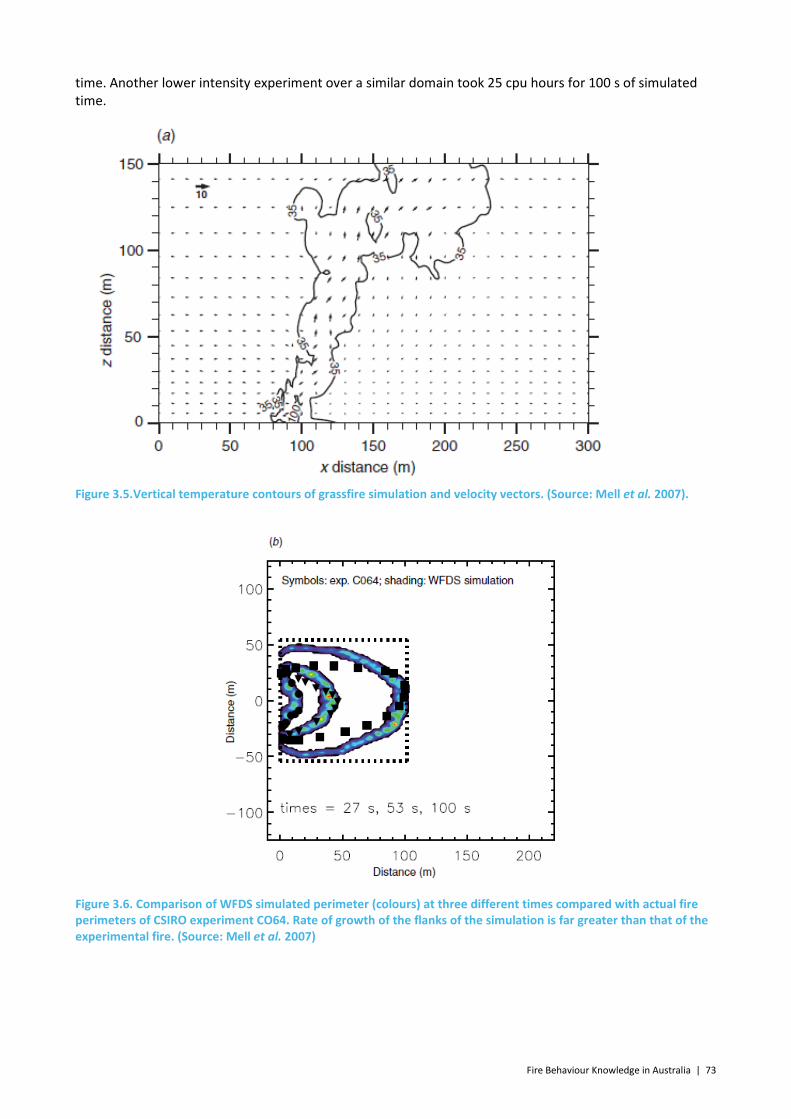
Fire Behaviour Knowledge in Australia | 73
time. Another lower intensity experiment over a similar domain took 25 cpu hours for 100 s of simulated time.
Figure 3.5.Vertical temperature contours of grassfire simulation and velocity vectors. (Source: Mell et al. 2007).
Figure 3.6. Comparison of WFDS simulated perimeter (colours) at three different times compared with actual fire perimeters of CSIRO experiment CO64. Rate of growth of the flanks of the simulation is far greater than that of the experimental fire. (Source: Mell et al. 2007)
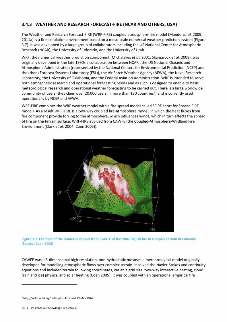
74 | Fire Behaviour Knowledge in Australia
3.4.3 WEATHER AND RESEARCH FORECAST-FIRE (NCAR AND OTHERS, USA)
The Weather and Research Forecast-FIRE (WRF-FIRE) coupled atmosphere-fire model (Mandel et al. 2009, 2011a) is a fire simulation environment based on a meso-scale numerical weather prediction system (Figure 3.7). It was developed by a large group of collaborators including the US National Center for Atmospheric Research (NCAR), the University of Colorado, and the University of Utah.
WRF, the numerical weather prediction component (Michalakes et al. 2001, Skamarock et al. 2008), was originally developed in the late 1990s a collaboration between NCAR , the US National Oceanic and Atmospheric Administration (represented by the National Centers for Environmental Prediction (NCEP) and the (then) Forecast Systems Laboratory (FSL)), the Air Force Weather Agency (AFWA), the Naval Research Laboratory, the University of Oklahoma, and the Federal Aviation Administration. WRF is intended to serve both atmospheric research and operational forecasting needs and as such is designed to enable to basic meteorological research and operational weather forecasting to be carried out. There is a large worldwide community of users (they claim over 20,000 users in more than 130 countries3
WRF-FIRE combines the WRF weather model with a fire spread model called SFIRE short for Spread FIRE model). As a result WRF-FIRE is a two-way coupled fire-atmosphere model, in which the heat fluxes from fire component provide forcing to the atmosphere, which influences winds, which in turn affects the spread of fire on the terrain surface. WRF-FIRE evolved from CAWFE (the Coupled-Atmosphere-Wildland Fire Environment (Clark et al. 2004; Coen 2005)).
) and is currently used operationally by NCEP and AFWA.
Figure 3.7. Example of the rendered output from CAWFE of the 2002 Big Elk fire in complex terrain in Colorado. (Source: Coen 2005).
CAWFE was a 3-dimensional high-resolution, non-hydrostatic mesoscale meteorological model originally developed for modelling atmospheric flows over complex terrain. It solved the Navier-Stokes and continuity equations and included terrain following coordinates, variable grid size, two-way interactive nesting, cloud (rain and ice) physics, and solar heating (Coen 2005). It was coupled with an operational empirical fire
3 http://wrf-model.org/index.php. Accessed 13 May 2014.
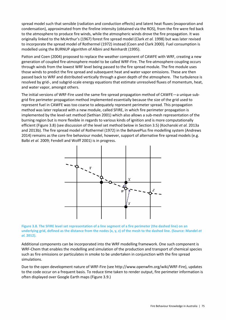
Fire Behaviour Knowledge in Australia | 75
spread model such that sensible (radiation and conduction effects) and latent heat fluxes (evaporation and condensation), approximated from the fireline intensity (obtained via the ROS), from the fire were fed back to the atmosphere to produce fire winds, while the atmospheric winds drove the fire propagation. It was originally linked to the McArthur’s (1967) forest fire spread model (Clark et al. 1998) but was later revised to incorporate the spread model of Rothermel (1972) instead (Coen and Clark 2000). Fuel consumption is modelled using the BURNUP algorithm of Albini and Reinhardt (1995).
Patton and Coen (2004) proposed to replace the weather component of CAWFE with WRF, creating a new generation of coupled fire-atmosphere model to be called WRF-Fire. The fire-atmosphere coupling occurs through winds from the lowest WRF level being passed to the fire spread module. The fire module uses those winds to predict the fire spread and subsequent heat and water vapor emissions. These are then passed back to WRF and distributed vertically through a given depth of the atmosphere. The turbulence is resolved by grid-, and subgrid-scale energy equations that estimate unresolved fluxes of momentum, heat, and water vapor, amongst others.
The initial versions of WRF-Fire used the same fire spread propagation method of CAWFE—a unique sub-grid fire perimeter propagation method implemented essentially because the size of the grid used to represent fuel in CAWFE was too coarse to adequately represent perimeter spread. This propagation method was later replaced with a new module, called SFIRE, in which fire perimeter propagation is implemented by the level-set method (Sethian 2001) which also allows a sub-mesh representation of the burning region but is more flexible in regards to various kinds of ignition and is more computationally efficient (Figure 3.8) (see discussion of the level set method below in Section 3.5) (Kochanski et al. 2013a and 2013b). The fire spread model of Rothermel (1972) in the BehavePlus fire modelling system (Andrews 2014) remains as the core fire behaviour model, however, support of alternative fire spread models (e.g. Balbi et al. 2009; Fendell and Wolff 2001) is in progress.
Figure 3.8. The SFIRE level set representation of a line segment of a fire perimeter (the dashed line) on an underlying grid, defined as the distance from the nodes (x, y, z) of the mesh to the dashed line. (Source: Mandel et al. 2012).
Additional components can be incorporated into the WRF modelling framework. One such component is WRF-Chem that enables the modelling and simulation of the production and transport of chemical species such as fire emissions or particulates in smoke to be undertaken in conjunction with the fire spread simulations.
Due to the open development nature of WRF-Fire (see http://www.openwfm.org/wiki/WRF-Fire), updates to the code occur on a frequent basis. To reduce time taken to render output, fire perimeter information is often displayed over Google Earth maps (Figure 3.9.)
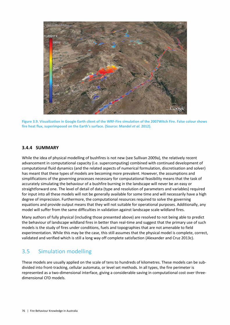
76 | Fire Behaviour Knowledge in Australia
Figure 3.9. Visualization in Google Earth client of the WRF-Fire simulation of the 2007Witch Fire. False colour shows fire heat flux, superimposed on the Earth’s surface. (Source: Mandel et al. 2012).
3.4.4 SUMMARY
While the idea of physical modelling of bushfires is not new (see Sullivan 2009a), the relatively recent advancement in computational capacity (i.e. supercomputing) combined with continued development of computational fluid dynamics (and the related aspects of numerical formulation, discretisation and solver) has meant that these types of models are becoming more prevalent. However, the assumptions and simplifications of the governing processes necessary for computational feasibility means that the task of accurately simulating the behaviour of a bushfire burning in the landscape will never be an easy or straightforward one. The level of detail of data (type and resolution of parameters and variables) required for input into all these models will not be generally available for some time and will necessarily have a high degree of imprecision. Furthermore, the computational resources required to solve the governing equations and provide output means that they will not suitable for operational purposes. Additionally, any model will suffer from the same difficulties in validation against landscape scale wildland fires.
Many authors of fully physical (including those presented above) are resolved to not being able to predict the behaviour of landscape wildland fires in better than real-time and suggest that the primary use of such models is the study of fires under conditions, fuels and topographies that are not amenable to field experimentation. While this may be the case, this still assumes that the physical model is complete, correct, validated and verified which is still a long way off complete satisfaction (Alexander and Cruz 2013c).
3.5 Simulation modelling
These models are usually applied on the scale of tens to hundreds of kilometres. These models can be sub-divided into front-tracking, cellular automata, or level set methods. In all types, the fire perimeter is represented as a two-dimensional interface, giving a considerable saving in computational cost over three-dimensional CFD models.

Fire Behaviour Knowledge in Australia | 77
Front tracking
In the front-tracking approach, the fire perimeter is described as a discretised set of line segments that expand according to a given rate-of-spread rule set. Each point on the fire perimeter is assumed to be a point source for future fire propagation (Knight and Coleman 1993; Finney 1994; Richards and Bryce 1996; Coleman and Sullivan 1996). The fire shape from these point sources are usually assumed to be elliptical, as ellipses have been found to provide a good approximation to fire perimeters in long-burning wild fires (Anderson et al. 1982; Richards 1990). The geometry of the ellipse is determined using a one dimensional rate of spread from an empirical relation for the length-to-breadth ratio of the ellipse (e.g. Alexander 1985) and the duration of the simulation time step. The symmetric nature of the template ellipse in conjunction with the application of Huygens' wavelet principle neatly provides the flank and rear spread of a fire. By relating the flank and rear spread through the ellipse geometry, the single rate of forward spread of the fire is all that is needed to simulate the spread of the entire perimeter.
The orientation of the ellipse is usually determined from wind direction. Topographic slope may also play a role (Finney 2004; Sharples 2008). The fire perimeter is updated as the maximum extent of all contributing fire ellipses for the time step.
Although these models are very fast, limitations arise from the use of only one type of front shape. While elliptical templates provides a close match to many fire propagation scenarios, other template shapes can provide a better match under certain circumstances (Green et al. 1983). For example, different fuels can produce ovoid (Peet 1967) or teardrop shaped fronts. French (1990) found that in homogeneous fuels and weather conditions, the Huygens' wavelet principle using the ellipse template shape suitably modelled fire spread, with only small distortion of the fire shape.
However, such a method cannot adequately handle conditions and fuels that are heterogeneous (e.g. they make the assumption of static conditions at each point on the perimeter for the period of the time step, and the assumption of instantaneous steady-state motion of the fire perimeter from a point source ignition) and errors are introduced through changes in the conditions during the time-step period as well as distortions in the fire perimeter due to artefacts in the Huygens' wavelet method. A large number of topology dependent rules are often required in these models to resolve overlapping, twisting or colliding fronts (Knight and Coleman 1993; Filippi et al. 2010; Bose et al. 2009). Models using this approach include SiroFire (Coleman and Sullivan 1995 1996), Phoenix (Tolhurst et al. 2008), Prometheus (Tymstra et al. 2010) and FARSITE (Finney 1998).
Cellular methods
Cellular methods discretise the domain into an underlying grid over which all input data is prescribed and all calculations are performed. Rule sets based on empirical or physical formula are used to update the state of the grid over time. Such models include static raster implementations (Green et al. 1990), cellular automata models (Encinas et al. 2007; Achtemeier 2013) and complex irregular stencil-based models (Trunfio et al. 2011). Examples of models using elliptical stencils include FireStation (Lopes et al. 2002), FIREMAP (Vasconcelos and Guertin 1992), and PYROCART (Perry et al. 1999).
Level set methods
A more recent approach, is perimeter-growth based on the level set method (Sethian 2001). In this method a local rate of spread can be applied at any point on the fire perimeter. Topological changes, such as breaking and merging of perimeters, are handled without the need for any rule sets to handle merging interfaces.
The method is also not reliant on the application of any pre-determined templates, such as ellipses. Implementations of such methods appear to be in the early stages of development compared to cellular and front-tracking methods. An early implementation was given by Rehm and McDermott (2009), who applied the method to a level homogenous terrain. Ignition points were found to evolve naturally into an elliptical form, showing the potential of the method for realistic fire perimeter simulation.
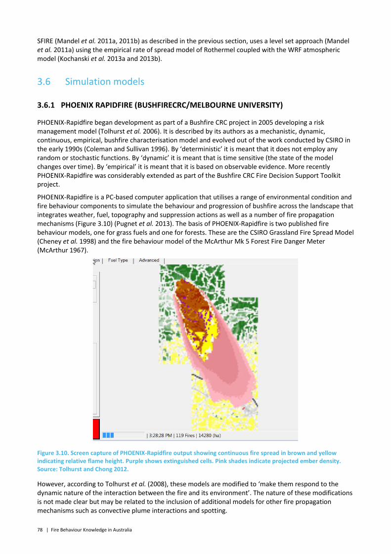
78 | Fire Behaviour Knowledge in Australia
SFIRE (Mandel et al. 2011a, 2011b) as described in the previous section, uses a level set approach (Mandel et al. 2011a) using the empirical rate of spread model of Rothermel coupled with the WRF atmospheric model (Kochanski et al. 2013a and 2013b).
3.6 Simulation models
3.6.1 PHOENIX RAPIDFIRE (BUSHFIRECRC/MELBOURNE UNIVERSITY)
PHOENIX-Rapidfire began development as part of a Bushfire CRC project in 2005 developing a risk management model (Tolhurst et al. 2006). It is described by its authors as a mechanistic, dynamic, continuous, empirical, bushfire characterisation model and evolved out of the work conducted by CSIRO in the early 1990s (Coleman and Sullivan 1996). By ‘deterministic’ it is meant that it does not employ any random or stochastic functions. By ‘dynamic’ it is meant that is time sensitive (the state of the model changes over time). By ‘empirical’ it is meant that it is based on observable evidence. More recently PHOENIX-Rapidfire was considerably extended as part of the Bushfire CRC Fire Decision Support Toolkit project.
PHOENIX-Rapidfire is a PC-based computer application that utilises a range of environmental condition and fire behaviour components to simulate the behaviour and progression of bushfire across the landscape that integrates weather, fuel, topography and suppression actions as well as a number of fire propagation mechanisms (Figure 3.10) (Pugnet et al. 2013). The basis of PHOENIX-Rapidfire is two published fire behaviour models, one for grass fuels and one for forests. These are the CSIRO Grassland Fire Spread Model (Cheney et al. 1998) and the fire behaviour model of the McArthur Mk 5 Forest Fire Danger Meter (McArthur 1967).
Figure 3.10. Screen capture of PHOENIX-Rapidfire output showing continuous fire spread in brown and yellow indicating relative flame height. Purple shows extinguished cells. Pink shades indicate projected ember density. Source: Tolhurst and Chong 2012.
However, according to Tolhurst et al. (2008), these models are modified to ‘make them respond to the dynamic nature of the interaction between the fire and its environment’. The nature of these modifications is not made clear but may be related to the inclusion of additional models for other fire propagation mechanisms such as convective plume interactions and spotting.

Fire Behaviour Knowledge in Australia | 79
PHOENIX-Rapidfire represents a fire perimeter as a series of linked points or vertices positioned across the landscape, known as a vector representation (each point is stored as a coordinate of the vector that represents the fire perimeter). The modified fire behaviour models are used to calculate the rate of forward spread, flame height and fireline intensity at each point around the perimeter and the perimeter expansion algorithm of Knight and Coleman (1993) is used to propagate the perimeter over the landscape for a fixed period (known as the time-step).
This perimeter propagation algorithm utilises Huygens’ wavelet principle (Anderson et al. 1982, Richards 1990) in which a template shape (in this case an ellipse) is placed at each vertex in the perimeter and a new perimeter generated by the combination of the extremities of each template. The geometry of the ellipse (i.e. length, width and orientation) is determined by the appropriate fire behaviour model for the fuel in question.
Fuel information is provided to PHOENIX-Rapidfire in the form of raster (i.e. cell-based) files exported from a geographic information system (GIS). Tools are provided to enable the export of these data from ARCMap or MapInfo software at the appropriate resolution (generally 30 m cell size). To improve computation times, higher resolution data cells are averaged over larger areas (Tolhurst and Chong 2012). Where multiple fuel types occur within a single cell, a weighted average of rate of spread predictions for all fuels present is calculated (Chong and Tolhurst 2012).
PHOENIX-Rapidfire can incorporate three sources of weather:
• historical weather files that may be produced externally or manually entered within the software, • automatic weather station feeds, or • gridded forecast data obtained directly from the Bureau of Meteorology.
Weather from multiple simultaneous sources is combined with the effects of terrain using the US Forest Service wind model WindNinja (Forthofer et al. in press).
Version 4.0 of PHOENIX-Rapidfire included a simplified convective plume model that brought a parameterised 3D component into the 2D fire spread simulation of previous versions (Chong et al. 2012a). This model utilises the calculation of heat release, identification of ‘heat segments’ around the fire perimeter and the aggregation of these heat segments to form convective centres which are then used to generate convective plumes (Figure 3.11).
Figure 3.11. Illustration of PHOENIX-Rapidfire simulation of three fires that have merged with three primary convective centres formed by a number of smaller heat segments from the fire perimeters. (Source: Chong and Tolhurst 2012)
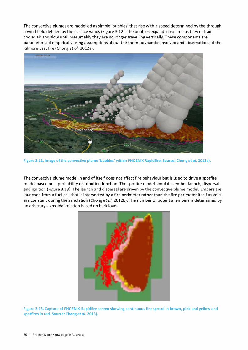
80 | Fire Behaviour Knowledge in Australia
The convective plumes are modelled as simple ‘bubbles’ that rise with a speed determined by the through a wind field defined by the surface winds (Figure 3.12). The bubbles expand in volume as they entrain cooler air and slow until presumably they are no longer travelling vertically. These components are parameterised empirically using assumptions about the thermodynamics involved and observations of the Kilmore East fire (Chong et al. 2012a).
Figure 3.12. Image of the convective plume ‘bubbles’ within PHOENIX Rapidfire. Source: Chong et al. 2012a).
The convective plume model in and of itself does not affect fire behaviour but is used to drive a spotfire model based on a probability distribution function. The spotfire model simulates ember launch, dispersal and ignition (Figure 3.13). The launch and dispersal are driven by the convective plume model. Embers are launched from a fuel cell that is intersected by a fire perimeter rather than the fire perimeter itself as cells are constant during the simulation (Chong et al. 2012b). The number of potential embers is determined by an arbitrary sigmoidal relation based on bark load.
Figure 3.13. Capture of PHOENIX-Rapidfire screen showing continuous fire spread in brown, pink and yellow and spotfires in red. Source: Chong et al. 2013).
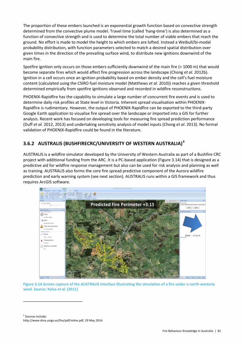
Fire Behaviour Knowledge in Australia | 81
The proportion of these embers launched is an exponential growth function based on convective strength determined from the convective plume model. Travel time (called ‘hang-time’) is also determined as a function of convective strength and is used to determine the total number of viable embers that reach the ground. No effort is made to model the height to which embers are lofted. Instead a Weibull/bi-modal probability distribution, with function parameters selected to match a desired spatial distribution over given times in the direction of the prevailing surface wind, to distribute new ignitions downwind of the main fire.
Spotfire ignition only occurs on those embers sufficiently downwind of the main fire (> 1000 m) that would become separate fires which would affect fire progression across the landscape (Chong et al. 2012b). Ignition in a cell occurs once an ignition probability based on ember density and the cell’s fuel moisture content (calculated using the CSIRO fuel moisture model (Matthews et al. 2010)) reaches a given threshold determined empirically from spotfire ignitions observed and recorded in wildfire reconstructions.
PHOENIX-Rapidfire has the capability to simulate a large number of concurrent fire events and is used to determine daily risk profiles at State level in Victoria. Inherent spread visualisation within PHOENIX-Rapidfire is rudimentary. However, the output of PHOENIX-Rapidfire can be exported to the third-party Google Earth application to visualise fire spread over the landscape or imported into a GIS for further analysis. Recent work has focused on developing tools for measuring fire spread prediction performance (Duff et al. 2012, 2013) and undertaking sensitivity analysis of model inputs (Chong et al. 2013). No formal validation of PHOENIX-Rapidfire could be found in the literature.
3.6.2 AUSTRALIS (BUSHFIRECRC/UNIVERSITY OF WESTERN AUSTRALIA)4
AUSTRALIS is a wildfire simulator developed by the University of Western Australia as part of a Bushfire CRC project with additional funding from the ARC. It is a PC-based application (
Figure 3.14) that is designed as a predictive aid for wildfire response management but also can be used for risk analysis and planning as well as training. AUSTRALIS also forms the core fire spread predictive component of the Aurora wildfire prediction and early warning system (see next section). AUSTRALIS runs within a GIS framework and thus requires ArcGIS software.
Figure 3.14.Screen capture of the AUSTRALIS interface illustrating the simulation of a fire under a north-westerly wind. Source: Kelso et al. (2011)
4 Sources include: http://www.dma.uvigo.es/fire/pdf/milne.pdf, 29 May 2014.
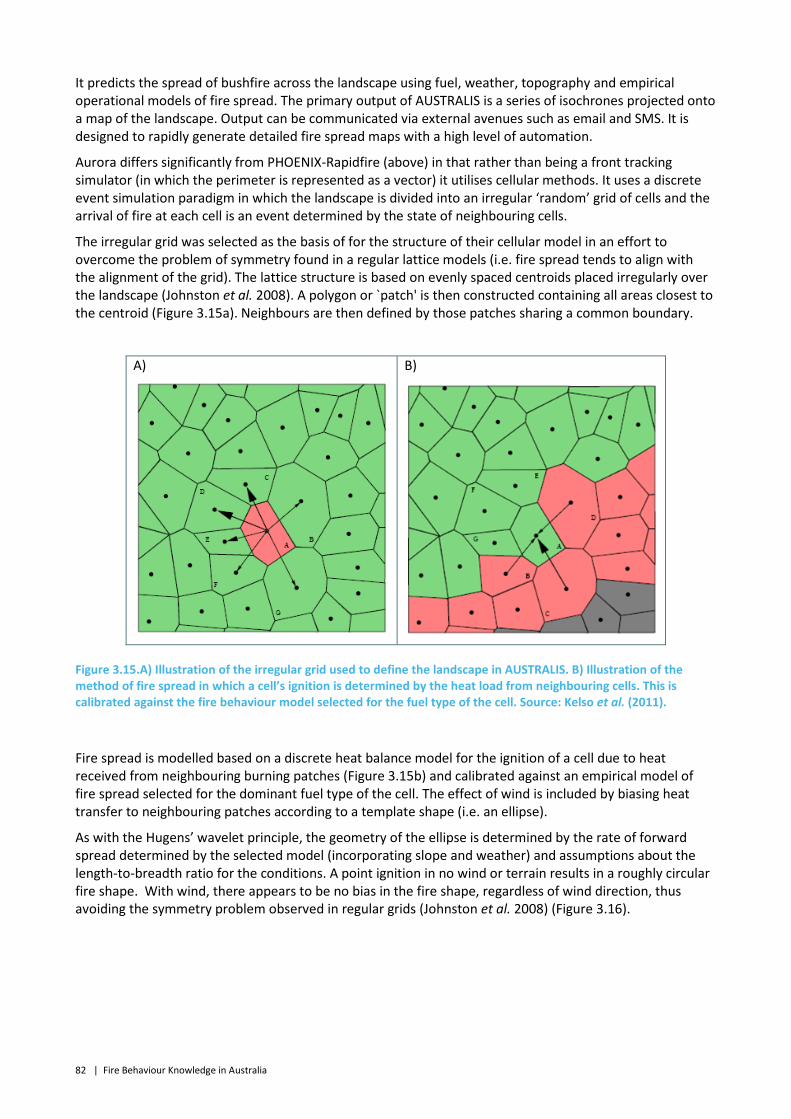
82 | Fire Behaviour Knowledge in Australia
It predicts the spread of bushfire across the landscape using fuel, weather, topography and empirical operational models of fire spread. The primary output of AUSTRALIS is a series of isochrones projected onto a map of the landscape. Output can be communicated via external avenues such as email and SMS. It is designed to rapidly generate detailed fire spread maps with a high level of automation.
Aurora differs significantly from PHOENIX-Rapidfire (above) in that rather than being a front tracking simulator (in which the perimeter is represented as a vector) it utilises cellular methods. It uses a discrete event simulation paradigm in which the landscape is divided into an irregular ‘random’ grid of cells and the arrival of fire at each cell is an event determined by the state of neighbouring cells.
The irregular grid was selected as the basis of for the structure of their cellular model in an effort to overcome the problem of symmetry found in a regular lattice models (i.e. fire spread tends to align with the alignment of the grid). The lattice structure is based on evenly spaced centroids placed irregularly over the landscape (Johnston et al. 2008). A polygon or `patch' is then constructed containing all areas closest to the centroid (Figure 3.15a). Neighbours are then defined by those patches sharing a common boundary.
A)
B)
Figure 3.15.A) Illustration of the irregular grid used to define the landscape in AUSTRALIS. B) Illustration of the method of fire spread in which a cell’s ignition is determined by the heat load from neighbouring cells. This is calibrated against the fire behaviour model selected for the fuel type of the cell. Source: Kelso et al. (2011).
Fire spread is modelled based on a discrete heat balance model for the ignition of a cell due to heat received from neighbouring burning patches (Figure 3.15b) and calibrated against an empirical model of fire spread selected for the dominant fuel type of the cell. The effect of wind is included by biasing heat transfer to neighbouring patches according to a template shape (i.e. an ellipse).
As with the Hugens’ wavelet principle, the geometry of the ellipse is determined by the rate of forward spread determined by the selected model (incorporating slope and weather) and assumptions about the length-to-breadth ratio for the conditions. A point ignition in no wind or terrain results in a roughly circular fire shape. With wind, there appears to be no bias in the fire shape, regardless of wind direction, thus avoiding the symmetry problem observed in regular grids (Johnston et al. 2008) (Figure 3.16).
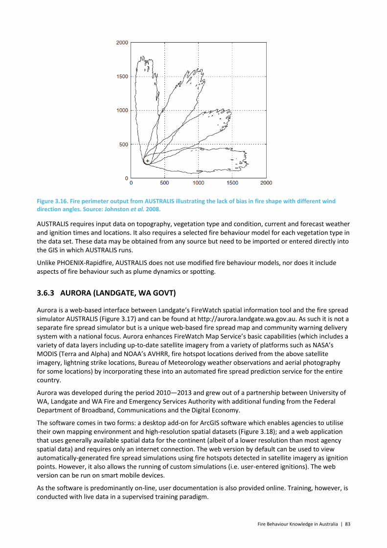
Fire Behaviour Knowledge in Australia | 83
Figure 3.16. Fire perimeter output from AUSTRALIS illustrating the lack of bias in fire shape with different wind direction angles. Source: Johnston et al. 2008.
AUSTRALIS requires input data on topography, vegetation type and condition, current and forecast weather and ignition times and locations. It also requires a selected fire behaviour model for each vegetation type in the data set. These data may be obtained from any source but need to be imported or entered directly into the GIS in which AUSTRALIS runs.
Unlike PHOENIX-Rapidfire, AUSTRALIS does not use modified fire behaviour models, nor does it include aspects of fire behaviour such as plume dynamics or spotting.
3.6.3 AURORA (LANDGATE, WA GOVT)
Aurora is a web-based interface between Landgate’s FireWatch spatial information tool and the fire spread simulator AUSTRALIS (Figure 3.17) and can be found at http://aurora.landgate.wa.gov.au. As such it is not a separate fire spread simulator but is a unique web-based fire spread map and community warning delivery system with a national focus. Aurora enhances FireWatch Map Service’s basic capabilities (which includes a variety of data layers including up-to-date satellite imagery from a variety of platforms such as NASA’s MODIS (Terra and Alpha) and NOAA’s AVHRR, fire hotspot locations derived from the above satellite imagery, lightning strike locations, Bureau of Meteorology weather observations and aerial photography for some locations) by incorporating these into an automated fire spread prediction service for the entire country.
Aurora was developed during the period 2010—2013 and grew out of a partnership between University of WA, Landgate and WA Fire and Emergency Services Authority with additional funding from the Federal Department of Broadband, Communications and the Digital Economy.
The software comes in two forms: a desktop add-on for ArcGIS software which enables agencies to utilise their own mapping environment and high-resolution spatial datasets (Figure 3.18); and a web application that uses generally available spatial data for the continent (albeit of a lower resolution than most agency spatial data) and requires only an internet connection. The web version by default can be used to view automatically-generated fire spread simulations using fire hotspots detected in satellite imagery as ignition points. However, it also allows the running of custom simulations (i.e. user-entered ignitions). The web version can be run on smart mobile devices.
As the software is predominantly on-line, user documentation is also provided online. Training, however, is conducted with live data in a supervised training paradigm.

84 | Fire Behaviour Knowledge in Australia
Figure 3.17. Screen capture of the web-based interface of Aurora. Source: Allen 2013.
Figure 3.18. Screen capture of the ArcGIS version of Aurora. Source: Allen 2013.
Unlike the output of AUSTRALIS, Aurora with its focus on community warnings, presents fire simulation results in the form of maps of arrival time in two hour intervals (i.e. 0-2 hours, 2-4 hours, etc) for each cell in the underlying dataset (see Figure 3.18 ).
The automatic fire spread simulations of satellite-mapped ignition points produce 24 hour maps of arrival time usually within 45 minutes of satellite overpass. All of Australia is covered at least three times a day by MODIS. These simulations use gridded forecast weather and national vegetation maps based on the Major

Fire Behaviour Knowledge in Australia | 85
Vegetation Sub-groups of the National Vegetation Information System (sourced from the Federal Department of the Environment). These vegetation maps are 100 m x 100 m resolution for the continent and use 1 km point spacing (Steber 2012). User defined simulations use 250 m point spacing with a fuel grid size of 25 km × 25 km.
It is claimed (Steber 2012) that currently 30 different fire spread models can be used within Aurora, including the McArthur forest and grassland meters and the Dry Eucalypt Forest Fire Model (Project Vesta). However, it is not clear if multiple models simply represent different fuel states for a single core model (e.g. eaten-out, grazed and natural pastures for the CSIRO Grassland Fire Spread Meter). Some fuel accumulation modelling is done for some fuel types (e.g. shrublands and mallee-heath) based on time since last burn determined from the near real-time (i.e. every 9 hours) AVHRR fire scar satellite imagery.
Prior to using the software, uses must be granted access via a web-based request. Approval is given by the Department of Fire and Emergency Services (DFES) and generally requires completion of some form of training.
3.6.4 PROMETHEUS (CANADIAN CONSORTIUM)
The Canadian Wildland Fire Growth Model, Prometheus, was developed by a collaborative consortium of Canadian national and provincial agencies with responsibility for fire management and fire research in the country. These include the Province of Alberta Department of Sustainable Resource Development (lead agency), the Canadian Forest Service, and Brandon University (CWFGM 2009).It is endorsed for use nationally by the Canadian Interagency Forest Fire Centre. The continued development of the Prometheus application is coordinated by the Prometheus Project Steering Committee (CWFGM 2009).
The software was developed as a result of the need to develop, customise, and implement a physically-based, deterministic fire growth model that would allow operational and strategic assessments of spatial fire behaviour potential across the landscape nationally (CWFGM 2009). The project commenced in 1999 (Tymstra et al. 2010). The requirements were to utilise a spatially-explicit fire growth model to simulate fire spread across a landscape on an hourly or daily basis, demonstrate the application of the model in operational, real-time prediction of fire growth of escaped wildfires, use it strategically determine the potential threat that an individual wildfire or multiple wildfires may pose to selected values-at-risk and the effectiveness of possible mitigative strategies (e.g. fuel management). The model was to be a standalone application that was easy to use and integrate with other applications.
As a result, Prometheus is a deterministic model based on the Canadian Fire Weather Index System (Van Wagner 1987) and the Canadian Forest Fire Behaviour Prediction Systems (FCFDG 1992, Wotton et al. 2009), modules of the larger Canadian Forest Fire Danger Rating System (CFFDRS) (Taylor and Alexander 2006). It is Windows-based and is intended for use as a real-time operational management tool (Figure 3.19). Version 1.0 was released in 2002 and in January 2013, version 5.5.0 was released. Later versions incorporated fire behaviour models specifically modified for New Zealand fuel types.
Prometheus utilises the front tracking (Huygens’ wavelet) propagation algorithms of Richards (1995) and Richards and Bryce (1996), employing an ellipse template shape to simulate fire perimeter propagation. The application models diurnal weather (temperature, relative humidity, wind speed) from input weather data and uses fuel and geographic data exported from third-party GIS platforms (such as ArcGIS and GRASS). Prometheus also allows the user to enter and edit fuel and meteorological data in the application.
Considerable effort was expended to ensure the program could be used across Canada by not only fire management agencies, but also by other interested stakeholders, such as landscape modellers, university researchers, forest management planners, municipal planners, and educators (ref user manual).
The program is written in Visual C++ and uses Microsoft’s Component Object Model (COM) interface.

86 | Fire Behaviour Knowledge in Australia
Figure 3.19. Screen capture of the Prometheus interface showing fire spread simulation perimeters over fuel information. Source: CWFGM 2009.
Extensive research into improving the fire perimeter propagation algorithms continues across agencies and universities involved in the project. A number of these focus on the mathematical aspects of the methods used and attempts to improve efficiency and effectiveness (e.g. Bose et al. 2009).
The Prometheus application and related software COM interface are shareware software and are available from http://www.firegrowthmodel.com
3.7 Operational evaluations
The software described in the preceding sections have been available in various forms for a number of years. In that time a number of agencies, either individually or collectively, have investigated the potential for deploying the applications for operational purposes and some have deployed them in such roles. While there has been no direct comparison of software performance (which was outside the scope of this project), some agencies have undertaken some validation activities against historical fires for one or more of the software available. However, only two reports could be obtained. These are summarised here. In addition, prior to the selection of a fire perimeter propagation model for national use in New Zealand in 2006, an international workshop was held (Opperman et al. 2006; Pearce 2009) where software developers compared model performance against a common dataset and pertinent results are summarised here.
Cook et al. (2009) undertook a summary assessment of both fire behaviour models and fire spread propagation models applicable to NSW for the NSW Rural Fire Service in which they conducted analysis of the performance of Phoenix against a limited set of historical fires in a range of fuels and burning conditions. They determined six requirements for a ‘good’ operational perimeter propagation system: accuracy, ease of use, meaningful output, speed, flexibility and level of support.
Their conclusion was that while Phoenix simulated the direction of spread reasonably well, it did rather poorer on simulating arrival time of the front, both over-predicting and under-predicting. They determined that while Phoenix could be difficult to understand, it was easily adaptable and simple to learn and it was simple to set up required data layers (with the exception of suppression). The gridded output of Phoenix provides large amounts of data suitable for a range of analyses but is not suitable for producing maps of fire isochrones due to the form of data being ‘unmanageable’. In terms of speed, set up can be time
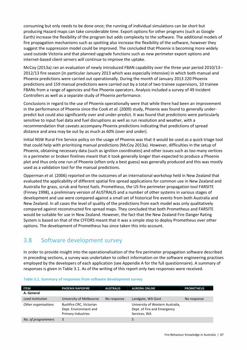
Fire Behaviour Knowledge in Australia | 87
consuming but only needs to be done once; the running of individual simulations can be short but producing Hazard maps can take considerable time. Export options for other programs (such as Google Earth) increase the flexibility of the program but adds complexity to the software. The additional models of fire propagation mechanisms such as spotting also increase the flexibility of the software, however they suggest the suppression model could be improved. The concluded that Phoenix is becoming more widely used outside Victoria and that planned upgrade functions such as new perimeter export options and internet-based client servers will continue to improve the uptake.
McCoy (2013a) ran an evaluation of newly introduced FBAN capability over the three year period 2010/13--2012/13 fire season (in particular January 2013 which was especially intensive) in which both manual and Phoenix predictions were carried out operationally. During the month of January 2013 220 Phoenix predictions and 159 manual predictions were carried out by a total of two trainee supervisors, 10 trainee FBANs from a range of agencies and five Phoenix operators. Analysis included a survey of 49 Incident Controllers as well as a separate study of Phoenix performance.
Conclusions in regard to the use of Phoenix operationally were that while there had been an improvement in the performance of Phoenix since the Cook et al. (2009) study, Phoenix was found to generally under-predict but could also significantly over and under-predict. It was found that predictions were particularly sensitive to input fuel data and fuel disruptions as well as run resolution and weather, with a recommendation that caveats accompany Phoenix predictions indicating that predictions of spread distance and area may be out by as much as 60% (over and under).
Initial NSW Rural Fire Service policy on the usage of Phoenix was that it would be used as a quick triage tool that could help with prioritising manual predictions (McCoy 2013a). However, difficulties in the setup of Phoenix, obtaining necessary data (such as ignition coordinates) and other issues such as too many vertices in a perimeter or broken firelines meant that it took generally longer than expected to produce a Phoenix plot and thus only one run of Phoenix (often only a best guess) was generally produced and this was mostly used as a validation tool for the manual predictions.
Opperman et al. (2006) reported on the outcomes of an international workshop held in New Zealand that evaluated the applicability of different spatial fire spread applications for common use in New Zealand and Australia for grass, scrub and forest fuels. Prometheus, the US fire perimeter propagation tool FARSITE (Finney 1998), a preliminary version of AUSTRALIS and a number of other systems in various stages of development and use were compared against a small set of historical fire events from both Australia and New Zealand. In all cases the level of quality of the predictions from each model was only qualitatively compared against reconstructed fire spread maps. They concluded that both Prometheus and FARSITE would be suitable for use in New Zealand. However, the fact that the New Zealand Fire Danger Rating System is based on that of the CFFDRS meant that it was a simple step to deploy Prometheus over other options. The development of Prometheus has since taken this into account.
3.8 Software development survey
In order to provide insight into the operationalisation of the fire perimeter propagation software described in preceding sections, a survey was undertaken to collect information on the software engineering practises employed by the developers of each application (see Appendix A for the full questionnaire). A summary of responses is given in Table 3.1. As of the writing of this report only two responses were received.
Table 3.1. Summary of responses from software development survey
ITEM PHOENIX RAPIDFIRE AUSTRALIS AURORA ONLINE PROMETHEUS A. General Lead institution University of Melbourne No response Landgate, WA Govt No response Other organisations Bushfire CRC, Victorian
Dept. Environment and Primary Industries
University of Western Australia, Dept. of Fire and Emergency Services, WA
No. of programmers 3 5

88 | Fire Behaviour Knowledge in Australia
ITEM PHOENIX RAPIDFIRE AUSTRALIS AURORA ONLINE PROMETHEUS Development language
Visual Basic.NET Aurora Web Application= PHP, JavaScript; Aurora MapServer Backend = PHP, Python; Aurora Processing Application = C,Shell Script, Australis Simulator=Java
Primary platform Windows 32-bit and 64-bit ( Phoenix engine can be run under Linux/other OS using Mono .NET)
Windows, Linux
Current release version
4.0.0.0 NA
Current development version
4.0.0.7 NA
B. Fire modelling Fuel types incorporated
Grasslands and sedgelands; all other fuel types considered by strata and equivalent fuel load
Within Australis, refer to UWA
Fire behaviour models incorporated
Modified CSIRO grassland model for grasslands; Novel dynamic fire behaviour model for other fuel types. Elements of McArthur Mk 5 Forest Fire Danger Meter used.
Within Australis, refer to UWA
Fire perimeter propagation method
Huygens as per Knight and Coleman (1993)
Within Australis, refer to UWA
Time for simulation of 100,000 ha fire.
< 5 mins at 180 m resolution on state wide dataset using 3.5 GHz single core machine
C. Cross-platform availability Other operating systems
None Any Web-enabled OS inc. desktop and mobile
D. Documentation Developer documentation
Automatically generated from source code
Manual creation by developer
User documentation Inline help, user manual, training guide
Online documentation (PDF), limited in-line help. No installation reqd as web-app.
E. Source control Code repository GIT, managed by
contractors at DEPI Subversion (SVN)
Release strategy Annual release with hot fixes as required. Currently stable product with only minor/infrequent enhancements
New releases are pulled from trunk with branching taken care of on the development server. Releases are pushed periodically via Phing build scripts.
Code merging None Developers have one or more local copies of the application running on a development server and typically only work on one feature per application at a time.

Fire Behaviour Knowledge in Australia | 89
ITEM PHOENIX RAPIDFIRE AUSTRALIS AURORA ONLINE PROMETHEUS Workflow for multiple platforms
None As software is web-based, only one code base required for multiple platforms.
F. Release management Strategy Release as needed to key
users Phing-based build scripts
extract latest copy from SVN, minifying and packaging code for publication on web server
User tracking None Yes Semantic version strategy
Yes No
Release process Email of zipped package to key users
Automatically deployed on web server
G. Integration and testing Auto compilation No NA Dedicated build server No NA Unit testing As needed Automated scripts poll the web
servers and the web mapping architecture backend to ensure web mapping OGC requests are successful and send SMS alerts if they fail
H. Bug tracking/source integration Bug tracker Yes Yes Integrated with source
Yes No
Tracked in source No No Bug fixes tracked in source
Manually Yes
Code review facility Yes Yes Algorithm checking No No Efficiency and effectiveness
Yes Manual
I. Planning and progress tracking Software development road map
Informal, not used to determine work schedule
No
Software improvement requirements
Determined by key end users and developers
User requested
Requirement management
Direct communication between manager and programmer
Prioritisation of user requests
Scheduled release targets
Annual release cycle As required by users and set priorities
Source code maintainability
Back up coder Good documentation
J. System testing Dedicated tester Programmer Development team Testing Load testing, comparison
of simulations against well-known datasets, real-time testing of reported and 9000+ static fires twice daily
Carried out within development, test and production environment
Software usability Not directly Yes Unit testing/ As required Yes
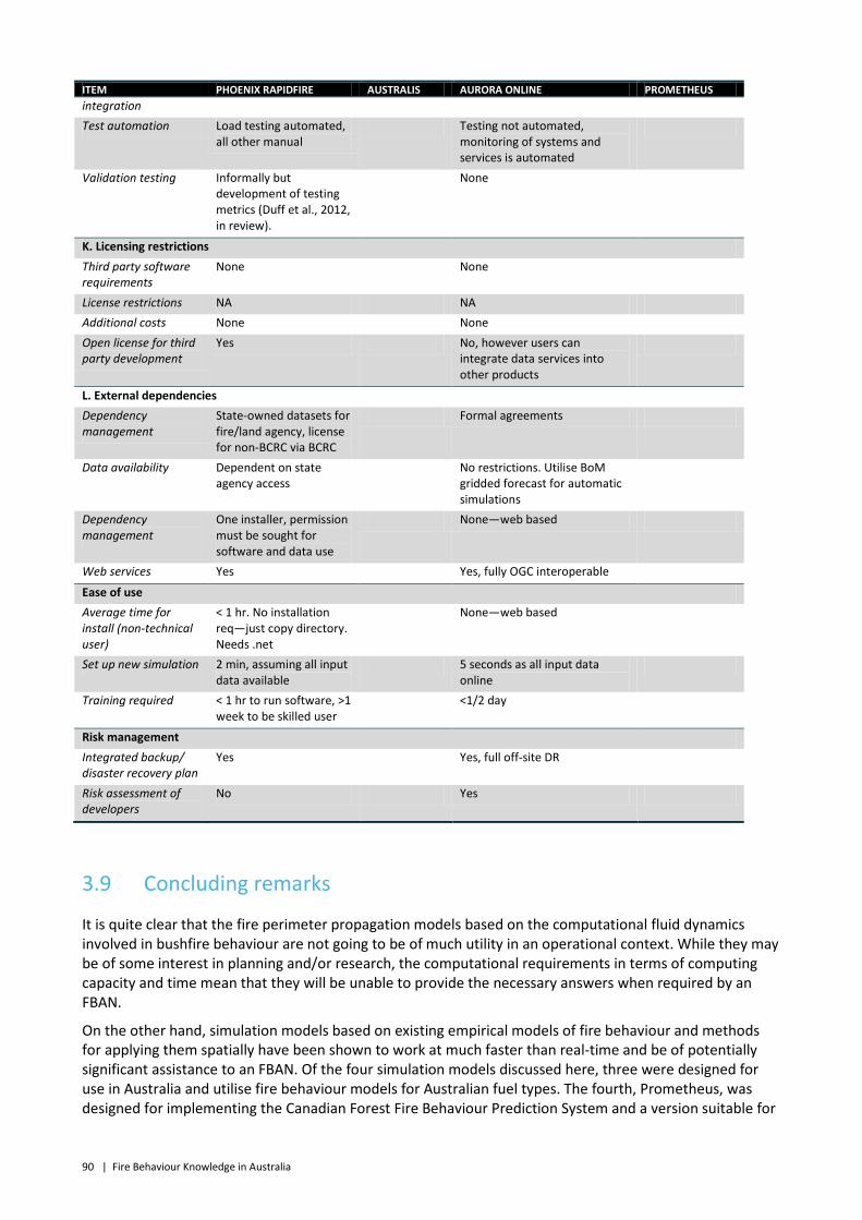
90 | Fire Behaviour Knowledge in Australia
ITEM PHOENIX RAPIDFIRE AUSTRALIS AURORA ONLINE PROMETHEUS integration Test automation Load testing automated,
all other manual Testing not automated,
monitoring of systems and services is automated
Validation testing Informally but development of testing metrics (Duff et al., 2012, in review).
None
K. Licensing restrictions Third party software requirements
None None
License restrictions NA NA Additional costs None None Open license for third party development
Yes No, however users can integrate data services into other products
L. External dependencies Dependency management
State-owned datasets for fire/land agency, license for non-BCRC via BCRC
Formal agreements
Data availability Dependent on state agency access
No restrictions. Utilise BoM gridded forecast for automatic simulations
Dependency management
One installer, permission must be sought for software and data use
None—web based
Web services Yes Yes, fully OGC interoperable
Ease of use Average time for install (non-technical user)
< 1 hr. No installation req—just copy directory. Needs .net
None—web based
Set up new simulation 2 min, assuming all input data available
5 seconds as all input data online
Training required < 1 hr to run software, >1 week to be skilled user
<1/2 day
Risk management Integrated backup/ disaster recovery plan
Yes Yes, full off-site DR
Risk assessment of developers
No Yes
3.9 Concluding remarks
It is quite clear that the fire perimeter propagation models based on the computational fluid dynamics involved in bushfire behaviour are not going to be of much utility in an operational context. While they may be of some interest in planning and/or research, the computational requirements in terms of computing capacity and time mean that they will be unable to provide the necessary answers when required by an FBAN.
On the other hand, simulation models based on existing empirical models of fire behaviour and methods for applying them spatially have been shown to work at much faster than real-time and be of potentially significant assistance to an FBAN. Of the four simulation models discussed here, three were designed for use in Australia and utilise fire behaviour models for Australian fuel types. The fourth, Prometheus, was designed for implementing the Canadian Forest Fire Behaviour Prediction System and a version suitable for

Fire Behaviour Knowledge in Australia | 91
use in New Zealand is deployed there. No forest fuel models within the Canadian system are applicable to Australian fuel types and therefore Prometheus is not recommended for use in Australian conditions.
PHOENIX-Rapidfire and AUSTRALIS (and thus Aurora which is based upon AUSTRALIS) are essentially the only models of choice currently available for Australian conditions. AUSTRALIS uses version of published fire behaviour models for a wide range of fuel types (about 30). In contrast, PHOENIX-Rapidfire uses two fire behaviour models, one modified from the CSIRO Grassland Fire Spread Model (for grassland and sedgeland fuels) and one for all other fuel types in which fuel components are stratified and fuel loads summed. The basis of this model is not clear but utilises in part the McArthur Mk 5 Forest Fire Danger Meter.
AUSTRALIS and the desktop version of Aurora are believed to require an ArcGIS license in order to operate. Most agencies have access to such a license so this should not be an issue. The web version of Aurora does not have this requirement and can be used using the provided datasets that are applicable nationally. However, it is understood that both AUSTRALIS and Aurora require a licensing agreement and certified training to be completed before the software can be used. PHOENIX-Rapidfire does not require a GIS to operate but geographic data must be sourced in the correct form from a GIS for it to be imported into the software.
PHOENIX-Rapidfire is essentially a completed software tool that is only being updated on an annual or needs basis with minor or infrequent enhancements as requested by key end users in discussion with the development team. No information about the state of the other software was forthcoming.
Agency evaluations of PHOENIX-Rapidfire suggest that it tends to under predict the spread of wildfires but can also significantly over and underpredict on occasion. However, the quality of a fire simulation prediction is highly dependent upon the quality of the data used to obtain it. Thus it would be very difficult to quantify the reasons for simulator performance given the large number of variables and spatial and temporal variation in those variables during the period of active fire spread.
Without conducting a detailed comparison of the performance of both the selection of fire behaviour models deployed in each model and the method of applying them spatially (which was beyond the scope of this project given the limitations in time and budget), the choice of selection of which model is most suited to FBAN use will be driven by consideration of a number of other factors. These include software licensing and data requirements, development pathways and software maintenance, software support and useability, and interoperability needs of the user organisation.
In order to determine suitability of fire simulation models it is suggested that extensive testing of possible models against a set of well-documented fire events across a broad range of burning and fuel conditions be undertaken by an independent assessment team utilising the range of performance metrics being developed for such purposes (e.g. Duff et al. 2012; Filippi et al.2013). It is further suggested that such comparisons of performance be carried out regularly as a form of independent testing of such models as they are continuously improved.

92 | Fire Behaviour Knowledge in Australia

Fire Behaviour Knowledge in Australia | 93
4 Fire Behaviour Analyst Practice: Survey and Interview
4.1 Introduction
‘Further major advances in combating wildfire are unlikely to be achieved simply by continued application of traditional methods. What is required is a more fundamental approach which can be applied at the design stage...Such an approach requires a detailed understanding of fire behaviour.’ (Drysdale 2011 p. 1).
Fire behaviour prediction science allows bushfire risk managers to forecast a potential version of the future, giving the ability to plan their method of mitigation prior to the realisation of an actual event (Gibos 2013a). It brings together a concrete analysis of the fire location (including topography and fuels) from a stance which is unaffected by cognitive biases, public pressure, and institutional incentive that can shape fire management (Thompson 2014). This union of the ‘art’ of reacting based on personal experience and the ‘science’ of technical bushfire behaviour prediction is the key to confident, informed decision-making under pressure. (Gibos 2013b). The move to a more scientific approach to fire prediction had led to numerous recent technical advances in bushfire behaviour analysis including Australian developments in computer software such as Phoenix and spatial fire behaviour forecast products using Bureau of Meteorology (BoM) gridded weather data.
The trend to a more scientific mode of fire behaviour prediction, however, requires adjustments within fire services. There has been a need for formal training of specialist fire behaviour analysts (FBANs) so a fire behaviour analyst course was initiated in Victoria in 2006 to fill the void by communicating academically reviewed scientific principles into everyday fire management activities. Since the inception of the training course, personnel from multiple fire management agencies have been trained and contributed products to facilitate tactical and strategic fire risk management decisions (Gibos 2013a). In NSW, a manual for fire prediction analysis has been produced (McCoy 2013b). There is scope for developing more complex but more reliable technologies based on ensemble predictions systems (EPS), which give output in terms of probabilities) however previous research suggests that the introduction of those systems might present further difficulties. For example, Handmer and Proudley (2007) found weather analysts disagreed about the meaning of probabilistic information and Demeritt et al. (2007) found that flood prediction analysts did not use the EPS information when it was provided in a workshop. Thus, the introduction of those more advanced systems would require further training of the FBANs and those who receive their predictions.
Many FBANs are working in an unprecedented climate of institutional change. In Victoria, the Bushfire Royal Commission commitments (Recommendation 17, Victorian Bushfires Royal Commission 2009) meant that all incident management team training courses must be suitable for all agencies, presenting a major challenge in bring agencies together with different training cultures, membership arrangements and responsibilities. A national Australasian Inter-Service Incident Management System (AIIMS) review has led to significant changes to the way the planning is conducted. There is also a push to focus emergency management on an ‘all hazards’ approach (Gibos 2013a).
Even in Victoria, a state which is a leading advocate for the use of specialist fire behaviour analysts, Gibos (2013b) identified three major problems facing bushfire services:
1. The need to clarify the role of the technical specialist fire behaviour analyst (FBAN) and how it will evolve into the future.
2. The lack of involvement and education of incident management personnel on methods for optimising the development, use and acceptance of FBAN products and services.
3. The limitations of current capability and capacity on FBAN services in the state.
94 | Fire Behaviour Knowledge in Australia
FBANs themselves have identified a range of challenges (Gibos 2013c). Many of these challenges were organisational in nature, such as a lack of a predictive services manager or coordinator. FBANs wanted support systems and contingencies for when they are overloaded (e.g. sending work to FBANs in other regions). Whether FBANs should be located in district offices or centrally located in the state office was an issue. This latter issue reflects another problem which is the shortage of trained FBANs. With more FBANs available, they could be located both centrally and regionally. Further, the lack of FBANs is exacerbated by the fact that other incident management team (IMT) roles offer a financial bonus and therefore have potential to direct people away from the FBAN role. Other problems were about a lack of recognition of the value of the new sophisticated techniques among incident managers or regional managers. In some cases managers preferred to rely on traditional methods and experience and in other cases they did not understand how to use the new information.
As analysis becomes increasingly technical, there is an increasing need for high levels of training and constant upgrading of skills. The Victorian Bushfires Royal Commission (2009) following the Black Saturday fires of February 2009 stressed the need to ‘provide regular training to IMT staff, highlighting the importance of information and reinforcing the support available from specialists within the State Control Centre’ (Recommendation 15). The Victorian FBANs in Gibos’ (2013c) study suggested that training should begin prior to FBAN training by developing the role of intelligence gatherer (measuring fuel condition, evaluation of fallback lines, provision of quality weather reporting from the fire line) to develop a set of basic skills to service the FBAN role. They also suggested that newly qualified FBANs then need to be nurtured through a system, such as a mentoring program, that encourages them to learn and keeps them interested and involved. This would require some management resources and ongoing support from the management. Further, all FBANs need opportunities to hone their skills, such as being involved in controlled burns, and regular hands-on updates in the use of new products. The technical nature of the role requires a level of commitment by the individual and the agency to maintain their skills. This is not readily achieved if the FBAN has a substantive role that is not fire related. The final area that needed attention was quick access to the input information when FBANs are called into a fire. For example, FBANs located at head offices need access to information from the fire site and ongoing maintenance is needed for the spreadsheets and data sources required as inputs for the modelling programs.
Thus the recent and rapid developments in diverse fire behaviour analysis techniques have led to a need for:
1. more, and more highly trained fire behaviour analysts
2. greater understanding of the available technologies
3. reconsideration of the organisational support, positioning and deployment of FBANs
4. a review of current specialist FBAN practices and requirements for assisting them to improve their performance.
The present research addresses the fourth issue: A review of current specialist FBAN practices and requirements for assisting them to improve their performance by conducting a survey of current FBAN practices and follow up interviews to address the requirements for assisting them to improve their performance. Given Gibos’ (2013c) findings, both technical and organisational issues will be addressed as part of the strategy for improving their performance.
The present project component was informed by CSIRO and international fire behaviour experts and an expert panel consisting of ten senior fire managers from New South Wales, Victoria, Tasmania, Western Australia, South Australia, Australian Capital Territory, and New Zealand.
4.2 Method
The data on fire behaviour analysts’ reports about their work was obtained from an online survey and telephone interviews. Ethical approval for the research was obtained from the CSIRO Ethics Committee Approval no. 010/14.

Fire Behaviour Knowledge in Australia | 95
4.2.1 ONLINE SURVEY
Content for the online survey was derived in large part from CSIRO and international bushfire behaviour experts supplemented by material from the Expert Panel and literature review. The Reference Panel also reviewed the survey as it was developed.
The survey consisted of seven major sections:
1. Background: demographic questions and their role as FBANs
2. Training: professional development and experience
3. Process: obtaining inputs for the analyses, communication with the personnel on the fire line and others, verification of predictions, timing of predictions and revisions
4. Fire prediction tools and simulation models
5. Inputs: air temperature, humidity, wind speed and direction, precipitation, fuel loads, topography
6. Outputs: content of reports
7. Review: reviewing fire analyses, confidence in their predictions.
The survey was detailed and lengthy with 101 questions (See Appendix B). The majority of questions were developed to have tick-box options as responses in order to reduce participant fatigue, although comment boxes were added to these questions to allow participants to clarify responses. The survey could be completed in about 40 minutes but most respondents put considerable effort into considering their answers and the completion of open-ended sections.
The survey was conducted online and data was gathered between 3/03/2014 and 28/04/2014.
4.2.2 TELEPHONE INTERVIEWS
Whereas the online survey consisted of detailed questions to collect a large amount of technical information, the telephone interviews were open-ended and gave FBANs the opportunity to discuss the issues that were important to them. The interview started by asking the FBANs to describe what typically happens when they are called to a fire: ‘I’d like to start by asking you to walk me through what happens when you get assigned to analyse a fire.’ The respondent was then encouraged to describe the whole process until the shift ends/the fire is controlled. The interviewer then went back over the account probing for difficulties and suggested improvements, for example ‘Ok, so you are called into the office – is that system working smoothly? Is there anything you would like to see improved? e.g. timeliness, allocation system.’ Probes were also based on the respondent’s survey responses, following up with any areas they identified as problems. In particular there were questions about their communication and connections and the support and recognition of their work.
Telephone interviews were approximately 45 minutes in length. Participants were advised that the telephone interview would be recorded and transcribed, and used to supplement information gathered in the survey.
4.2.3 PARTICIPANT RECRUITMENT
Participants were recruited via an invitation email. A list of potential participants was provided by the Reference Panel, who nominated FBANs from Australia and New Zealand who had a minimum of two years experience in the role and had undertaken predictions for at least two major fires.
A total of 54 fire behaviour analysts were emailed an invitation to participate, which included information about the project and a consent form. They were asked to return the completed consent form to indicate their willingness to participate and would in turn receive an email with a link to the online survey, along

96 | Fire Behaviour Knowledge in Australia
with an access code. This access code was to ensure participant information was separated from their responses.
Reminder emails were sent out during the collection period, both to nominees who had not yet returned a consent form and those who had returned a consent form but not yet completed the online survey. A total of 32 fire behaviour analysts completed the online survey.
In addition to the online survey, participants were advised they may be contacted for a telephone interview and were asked to provide a contact number and both suitable and unsuitable contact times. There were difficulties encountered in completing the telephone interviews, due in part to the unpredictable nature of the work undertaken by the analysts and the time required for the interview. In total, eight participants completed the in-depth telephone interviews.
4.2.4 PARTICIPANT DEMOGRAPHICS
A total of 32 fire behaviour analysts completed the online survey. While the majority of participants (53.1%) were from Victoria and New South Wales, there are participants from each Australian state as well as representatives from New Zealand, as detailed in Table 4.1 below.
Table 4.1 Location of survey participants
LOCATION PARTICIPANTS (N = 32)
%
VIC 9 28.1%
NSW 8 25.0%
WA 5 15.6%
TAS 4 12.5%
QLD 2 6.3%
NZ 2 6.3%
SA 1 3.1%
International - other 1 3.1%
The International-other representative has had significant experience in both New Zealand and Victoria, so the decision was made to invite the respondent to participate.
Figure 4.1 Age distribution of respondents.

Fire Behaviour Knowledge in Australia | 97
Most of the sample were men (n = 26), with women representing less than 20% (n = 6) of the total participants (Q 1). Over 60% (n = 20) of the participants were aged between 35 and 54, and a further 25% were in the 55–64 age category (Q 2). The age distribution is detailed below in Figure 4.1.
Table 4.2 details the survey respondents’ formal education (Q 3). All participants had undertaken further education, with nearly half having started or completed a postgraduate qualification (n = 4 and n = 11, respectively). A further 40.6% had completed an undergraduate degree, with the remaining 12.5% having completed a trade/TAFE qualification.
Table 4.2 Highest level of formal education
PARTICIPANTS
(N = 32) %
High school 0 0.0%
Trade/TAFE qualification 4 12.5%
Undergraduate degree 13 40.6%
Some of postgraduate qualification 4 12.5%
Postgraduate qualification 11 34.4%
All but one were in full time employment but only half (50%) worked full time as FBANs (
Q 6). One was a volunteer and the others worked part time as required in the fire season (Q 11). Nineteen worked with a land management agency and twelve with a fire authority (Q 8). All but eight worked in fire related paid work. The others had positions in land conservation or community safety more broadly (Q 5). One had retired from fire related work.
4.2.5 ANALYSIS
Data from the online survey and interviews was entered into an Excel spreadsheet for content analysis.
4.3 Results 1: The FBANs experience
Out of the 32 respondents, 31 were highly experienced in bushfire analysis and one was a researcher who was knowledgeable in the subject area but not had direct fire management experience. They had been working in the area of fire behaviour prediction for an average of 18.5 years (median 17 years 9 months; Q 13) with an average of 5 years (Q 12). The three least experienced individuals had been working on fire prediction for 3–5 years (Q 13). Some respondents were leaders in the field: designing fire behaviour based decision support tools and systems; being active in research; managing state-wide FBAN programs; or undertaking a leading role within the Australasian Fire and Emergency Service Authorities Council (AFAC) to establish a national FBAN capacity (Q 7).
Their experience could also be gauged by the number and size of fires they had analysed. Only six had analysed 5 or fewer fires and five had worked on 6–10 fires. Eight had worked on over 40 fires including some who had analysed hundreds of fires (Q 27). They had worked quite intensively covering multiple fires simultaneously. Sixteen had analysed 2–5 fires at a time; seven had worked on 6–12 and four had worked on over 10 fires at a time (Q 28). They had analysed substantial fires; the smallest being 12,500 hectares. Thirteen FBANs had analysed fires of over 100 000 hectares (Q 29).
The FBANs used a number of fire behaviour products that were standard for their organisations and 19 reported that their organisation had a handbook for FBANs (Q 22). Fire spread maps were standard behaviour products in almost all organisations and written reports were standard in 90%. About two-thirds also used potential impact zone maps (Q 23). Most organisations had a range of other standard products. For mapping products, three mentioned Phoenix, three used head fire intensity maps, three used time to 5
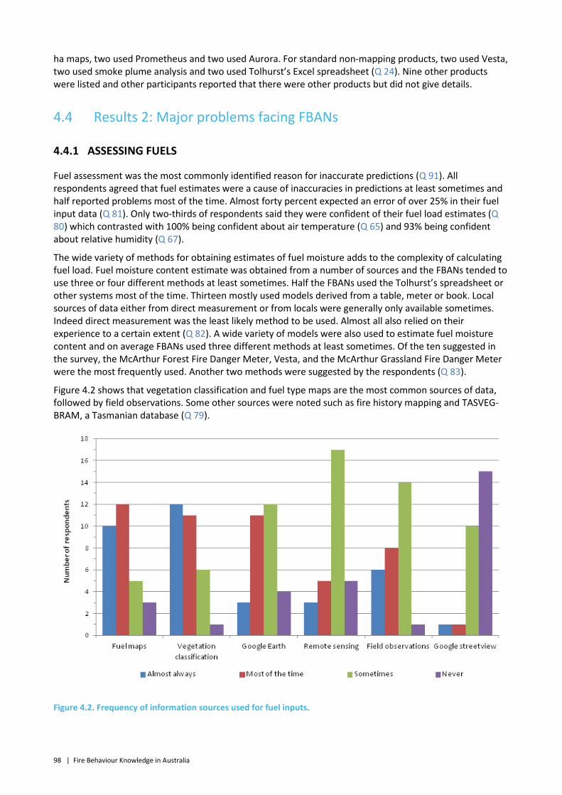
98 | Fire Behaviour Knowledge in Australia
ha maps, two used Prometheus and two used Aurora. For standard non-mapping products, two used Vesta, two used smoke plume analysis and two used Tolhurst’s Excel spreadsheet (Q 24). Nine other products were listed and other participants reported that there were other products but did not give details.
4.4 Results 2: Major problems facing FBANs
4.4.1 ASSESSING FUELS
Fuel assessment was the most commonly identified reason for inaccurate predictions (Q 91). All respondents agreed that fuel estimates were a cause of inaccuracies in predictions at least sometimes and half reported problems most of the time. Almost forty percent expected an error of over 25% in their fuel input data (Q 81). Only two-thirds of respondents said they were confident of their fuel load estimates (Q 80) which contrasted with 100% being confident about air temperature (Q 65) and 93% being confident about relative humidity (Q 67).
The wide variety of methods for obtaining estimates of fuel moisture adds to the complexity of calculating fuel load. Fuel moisture content estimate was obtained from a number of sources and the FBANs tended to use three or four different methods at least sometimes. Half the FBANs used the Tolhurst’s spreadsheet or other systems most of the time. Thirteen mostly used models derived from a table, meter or book. Local sources of data either from direct measurement or from locals were generally only available sometimes. Indeed direct measurement was the least likely method to be used. Almost all also relied on their experience to a certain extent (Q 82). A wide variety of models were also used to estimate fuel moisture content and on average FBANs used three different methods at least sometimes. Of the ten suggested in the survey, the McArthur Forest Fire Danger Meter, Vesta, and the McArthur Grassland Fire Danger Meter were the most frequently used. Another two methods were suggested by the respondents (Q 83).
Figure 4.2 shows that vegetation classification and fuel type maps are the most common sources of data, followed by field observations. Some other sources were noted such as fire history mapping and TASVEG-BRAM, a Tasmanian database (Q 79).
Figure 4.2. Frequency of information sources used for fuel inputs.
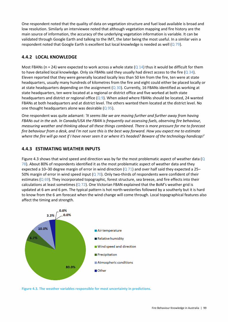
Fire Behaviour Knowledge in Australia | 99
One respondent noted that the quality of data on vegetation structure and fuel load available is broad and low resolution. Similarly an interviewee noted that although vegetation mapping and fire history are the main source of information, the accuracy of the underlying vegetation information is variable. It can be validated through Google Earth and talking to the IMT, the later being the most useful. In a similar vein a respondent noted that Google Earth is excellent but local knowledge is needed as well (Q 79).
4.4.2 LOCAL KNOWLEDGE
Most FBANs (n = 24) were expected to work across a whole state (Q 14) thus it would be difficult for them to have detailed local knowledge. Only six FBANs said they usually had direct access to the fire (Q 34). Eleven reported that they were generally located locally less than 50 km from the fire, ten were at state headquarters, usually many hundreds of kilometres from the fire and eight could either be placed locally or at state headquarters depending on the assignment (Q 30). Currently, 16 FBANs identified as working at state headquarters, ten were located at a regional or district office and five worked at both state headquarters and district or regional office (Q 9). When asked where FBANs should be located, 24 wanted FBANs at both headquarters and at district level. The others wanted them located at the district level. No one thought headquarters alone was desirable (Q 95).
One respondent was quite adamant: ‘It seems like we are moving further and further away from having FBANs out in the ash. In Canada/USA the FBAN is frequently out assessing fuels, observing fire behaviour, measuring weather and thinking about all these things combined. There is more pressure for me to forecast fire behaviour from a desk, and I'm not sure this is the best way forward. How you expect me to estimate where the fire will go next if I have never seen it or where it's headed? Beware of the technology handicap!’
4.4.3 ESTIMATING WEATHER INPUTS
Figure 4.3 shows that wind speed and direction was by far the most problematic aspect of weather data (Q 78). About 80% of respondents identified it as the most problematic aspect of weather data and they expected a 10–30 degree margin of error in wind direction (Q 71) and over half said they expected a 25–50% margin of error in wind speed input (Q 70). Only two-thirds of respondents were confident of their estimates (Q 69). They incorporated topographic, forest structure, sea breeze, and fire effects into their calculations at least sometimes (Q 72). One Victorian FBAN explained that the BoM’s weather grid is updated at 6 am and 6 pm. The typical pattern is hot north-westerlies followed by a southerly but it is hard to know from the 6 am forecast when the wind change will come through. Local topographical features also affect the timing and strength.
Figure 4.3. The weather variables responsible for most uncertainty in predictions.
100 | Fire Behaviour Knowledge in Australia
4.4.4 ATMOSPHERIC CONDITIONS
Some 10% of FBANs reported that atmospheric conditions were the aspect of weather that caused the highest level of uncertainty (Q 78). When asked about upper atmospheric conditions almost all used the Haines or C-Haines and most used the F160 as well (Q 76). Use of the F160 relies on suitable sites and one respondent reported that in his area one is too far away, and the other is to the north-east which is not useful for fire prediction. FBANs commented on the importance of understanding the likelihood of mixing down of upper level winds. Such an understanding helps predict, the risk of convective driven fires, spot fire potential, fire instability, and ‘blow up’ conditions thus assisting the FBAN to give appropriate warnings (Q 77).
4.4.5 PRECIPITATION
Although over half of the FBANs were confident (n = 16) or very confident (n = 2) of their precipitation inputs, a sizable minority (n = 11) were not confident about these estimates (Q 73). While most expected a margin of error of under three hours in the timing of the predictions, ten expected more than three hours or did not know the margin of error (Q 74). Two-thirds thought the margin of error in their prediction of the amount of precipitation was 5–15 ml and a third thought it was less than 5 ml (Q 75).
4.4.6 INCORPORATING SUPPRESSION EFFORTS
Forty percent of FBANs incorporated suppression activities into their predictions (Q 35). There is general agreement that suppression efforts are not properly taken into account in fire behaviour analysis and almost all respondents agreed that suppression efforts were a cause of inaccuracies in predictions at least sometimes (Q 91), but opinions vary about the problem:
• Some believed that this was not their role and that their role was to give the worst case scenario – as is NSW policy. One interview commented ‘But it does make it hard. It then puts all these questions in your mind about, well “I know that this trail or this river is going to slow this fire down. I know that there are helicopters working really effectively in this area”.’
• Others believe that assessing suppression effects is very difficult because of the problems obtaining accurate information about the suppression efforts.
• Phoenix has some capability to incorporate efforts along the fire flanks but this was seen as limited, for example, with helicopters spot fires and properties are targeted too, not just the flanks.
• Infra-red images of the fire are extremely useful and show effects of suppression but are they not always readily or frequently available. NSW Rural Fire Service increased IR line scans to 3–4 per day last season and FBANs have appreciated this.
Although the difference between the worst case and likely case scenarios does not rest entirely on the suppression efforts, they are a major factor. Half the FBANs preferred to make predictions for both the worst case and likely case scenarios, if time permits. Six favoured the worst case scenario and only two favoured the likely case scenario. Four said it depended on the context such as the consequences or the needs of the client. Thus, only the six who focussed solely on worst case scenarios did not need to take into account suppression efforts (Q 86).
4.4.7 ACCESSING DATA FROM ELECTRONIC SYSTEMS
Most of the time, FBANs do have access to the data they need (Figure 4.4) but most of the time it may not be good enough (Q 59). It suggests some unpredictability for FBANs in being able to properly do their work. In regional areas they reported that ‘it pays to take your own resources’. One problem was different departments which were not entirely synchronised. For example, National Parks and Wildlife Service (NPWS) cannot fully access the Rural Fire Service (RFS) databases in NSW. There can be delays setting up an RFS computer at busy times which is when NPWS is likely to be called in – but this is improving. Another
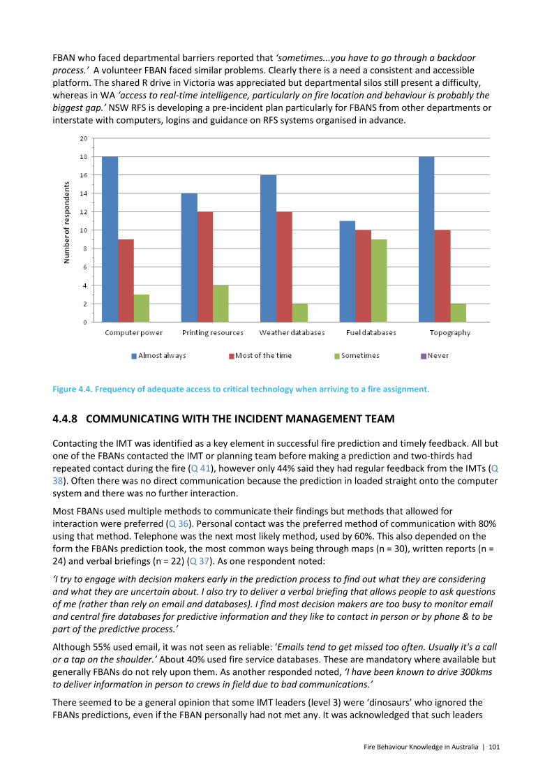
Fire Behaviour Knowledge in Australia | 101
FBAN who faced departmental barriers reported that ‘sometimes...you have to go through a backdoor process.’ A volunteer FBAN faced similar problems. Clearly there is a need a consistent and accessible platform. The shared R drive in Victoria was appreciated but departmental silos still present a difficulty, whereas in WA ‘access to real-time intelligence, particularly on fire location and behaviour is probably the biggest gap.’ NSW RFS is developing a pre-incident plan particularly for FBANS from other departments or interstate with computers, logins and guidance on RFS systems organised in advance.
Figure 4.4. Frequency of adequate access to critical technology when arriving to a fire assignment.
4.4.8 COMMUNICATING WITH THE INCIDENT MANAGEMENT TEAM
Contacting the IMT was identified as a key element in successful fire prediction and timely feedback. All but one of the FBANs contacted the IMT or planning team before making a prediction and two-thirds had repeated contact during the fire (Q 41), however only 44% said they had regular feedback from the IMTs (Q 38). Often there was no direct communication because the prediction in loaded straight onto the computer system and there was no further interaction.
Most FBANs used multiple methods to communicate their findings but methods that allowed for interaction were preferred (Q 36). Personal contact was the preferred method of communication with 80% using that method. Telephone was the next most likely method, used by 60%. This also depended on the form the FBANs prediction took, the most common ways being through maps (n = 30), written reports (n = 24) and verbal briefings (n = 22) (Q 37). As one respondent noted:
‘I try to engage with decision makers early in the prediction process to find out what they are considering and what they are uncertain about. I also try to deliver a verbal briefing that allows people to ask questions of me (rather than rely on email and databases). I find most decision makers are too busy to monitor email and central fire databases for predictive information and they like to contact in person or by phone & to be part of the predictive process.’
Although 55% used email, it was not seen as reliable: ‘Emails tend to get missed too often. Usually it's a call or a tap on the shoulder.’ About 40% used fire service databases. These are mandatory where available but generally FBANs do not rely upon them. As another responded noted, ‘I have been known to drive 300kms to deliver information in person to crews in field due to bad communications.’
There seemed to be a general opinion that some IMT leaders (level 3) were ‘dinosaurs’ who ignored the FBANs predictions, even if the FBAN personally had not met any. It was acknowledged that such leaders

102 | Fire Behaviour Knowledge in Australia
may have experienced some bad predictions and lost faith in the process. Therefore, there was a need to educate them about the value of FBAN predictions but also to be realistic about their limitations and assumptions e.g. making it clear that suppression efforts had not been taken into account. IMT leaders should not be expected to attend a five day course but could be given a two-page overview of the process and some idea of the confidence that can be expected around predictions.
Figure 4.5. Frequency of output variable inclusion in fire simulation report.
Some FBANs stressed the importance of ongoing communication with the IMT to obtain information about local conditions, and discuss their predictions and assumptions about the fuel type(s), etc. However, some IMT leaders were irritated at being bothered with requests for information by someone at state headquarters whom they saw as irrelevant. Other FBANs bypassed the official approval system to communicate directly with the IMT leaders when the situation was urgent and they were known and trusted. One interviewee suggested that when the FBAN service had matured, it would be providing information in a form that was most useful to the IMTs including advice on suppression tactics and responsive to IMT’s specific requests such as the time at which a fire would reach a particular site.
4.4.9 NEED FOR MORE TRAINING
Nearly half of the FBANs had undergone training within the last five years (Q 17), and most FBANs had completed a basic fire behaviour analysis course (Q 16). Half the FBANs said they needed further training (Q 18). They specifically mentioned further training in the latest prediction tools; the computer simulations (e.g. Phoenix or Aurora); choosing a model of best fit for the environmental conditions; explanation of all the assumptions implicit in the models; the need for an annual refresher course especially as the tools were constantly being updated; the tools used in other states (as over one-quarter of FBANs had been deployed interstate Q 15); and strategic and tactical analysis.
Almost all the FBANs would appreciate more time to work through cases/scenarios with other FBANs or instructors (Q 19). Reading case studies was OK, but face-to-face interactive analysis was most valued (Q 20). Part-timers, and those whose winter jobs were quite different, felt the greatest need to update their skills at the beginning of each season. The one-day pre-season orientation in Victoria and two-day
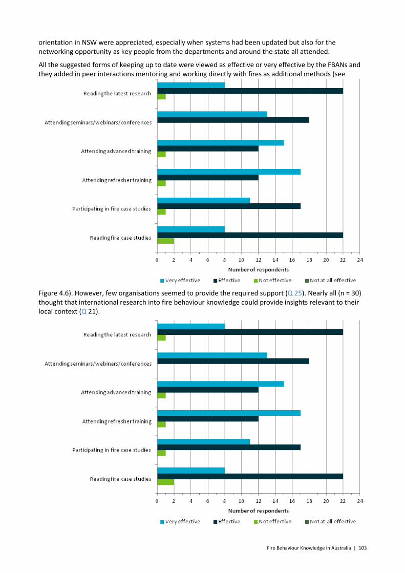
Fire Behaviour Knowledge in Australia | 103
orientation in NSW were appreciated, especially when systems had been updated but also for the networking opportunity as key people from the departments and around the state all attended.
All the suggested forms of keeping up to date were viewed as effective or very effective by the FBANs and they added in peer interactions mentoring and working directly with fires as additional methods (see
Figure 4.6). However, few organisations seemed to provide the required support (Q 25). Nearly all (n = 30) thought that international research into fire behaviour knowledge could provide insights relevant to their local context (Q 21).
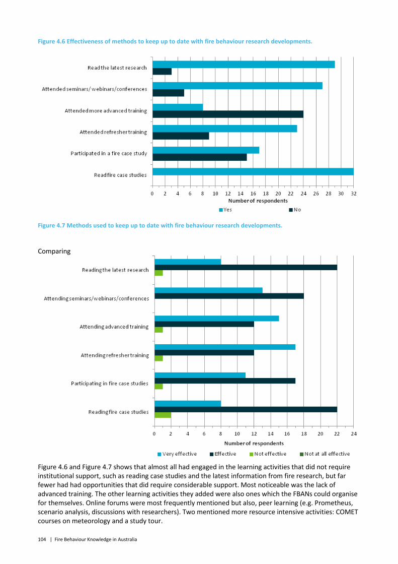
104 | Fire Behaviour Knowledge in Australia
Figure 4.6 Effectiveness of methods to keep up to date with fire behaviour research developments.
Figure 4.7 Methods used to keep up to date with fire behaviour research developments.
Comparing
Figure 4.6 and Figure 4.7 shows that almost all had engaged in the learning activities that did not require institutional support, such as reading case studies and the latest information from fire research, but far fewer had had opportunities that did require considerable support. Most noticeable was the lack of advanced training. The other learning activities they added were also ones which the FBANs could organise for themselves. Online forums were most frequently mentioned but also, peer learning (e.g. Prometheus, scenario analysis, discussions with researchers). Two mentioned more resource intensive activities: COMET courses on meteorology and a study tour.
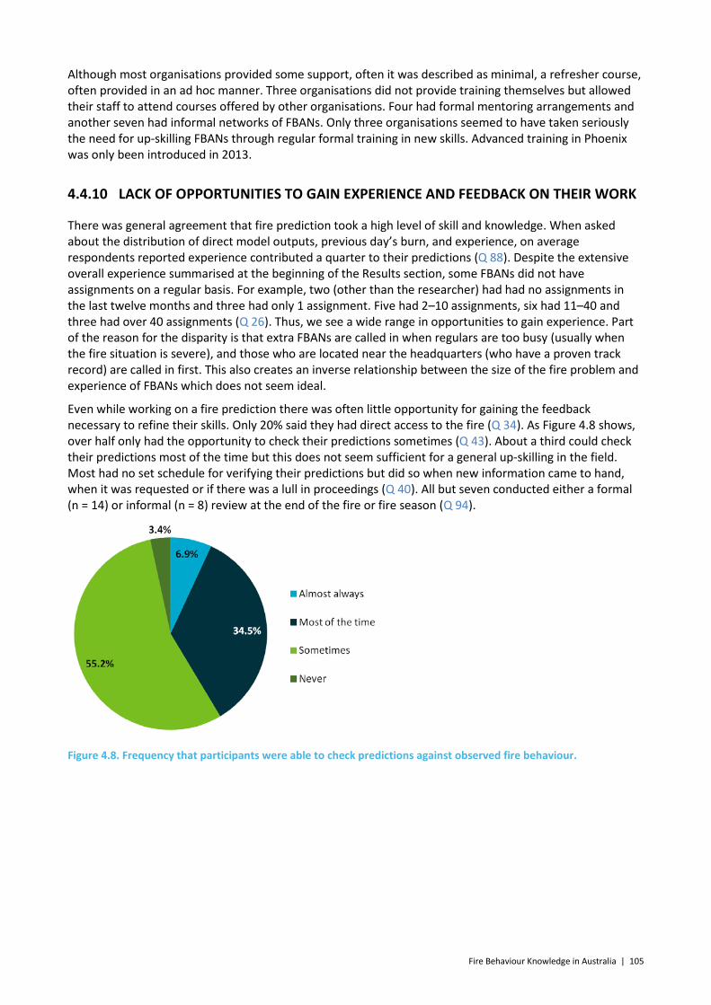
Fire Behaviour Knowledge in Australia | 105
Although most organisations provided some support, often it was described as minimal, a refresher course, often provided in an ad hoc manner. Three organisations did not provide training themselves but allowed their staff to attend courses offered by other organisations. Four had formal mentoring arrangements and another seven had informal networks of FBANs. Only three organisations seemed to have taken seriously the need for up-skilling FBANs through regular formal training in new skills. Advanced training in Phoenix was only been introduced in 2013.
4.4.10 LACK OF OPPORTUNITIES TO GAIN EXPERIENCE AND FEEDBACK ON THEIR WORK
There was general agreement that fire prediction took a high level of skill and knowledge. When asked about the distribution of direct model outputs, previous day’s burn, and experience, on average respondents reported experience contributed a quarter to their predictions (Q 88). Despite the extensive overall experience summarised at the beginning of the Results section, some FBANs did not have assignments on a regular basis. For example, two (other than the researcher) had had no assignments in the last twelve months and three had only 1 assignment. Five had 2–10 assignments, six had 11–40 and three had over 40 assignments (Q 26). Thus, we see a wide range in opportunities to gain experience. Part of the reason for the disparity is that extra FBANs are called in when regulars are too busy (usually when the fire situation is severe), and those who are located near the headquarters (who have a proven track record) are called in first. This also creates an inverse relationship between the size of the fire problem and experience of FBANs which does not seem ideal.
Even while working on a fire prediction there was often little opportunity for gaining the feedback necessary to refine their skills. Only 20% said they had direct access to the fire (Q 34). As Figure 4.8 shows, over half only had the opportunity to check their predictions sometimes (Q 43). About a third could check their predictions most of the time but this does not seem sufficient for a general up-skilling in the field. Most had no set schedule for verifying their predictions but did so when new information came to hand, when it was requested or if there was a lull in proceedings (Q 40). All but seven conducted either a formal (n = 14) or informal (n = 8) review at the end of the fire or fire season (Q 94).
Figure 4.8. Frequency that participants were able to check predictions against observed fire behaviour.
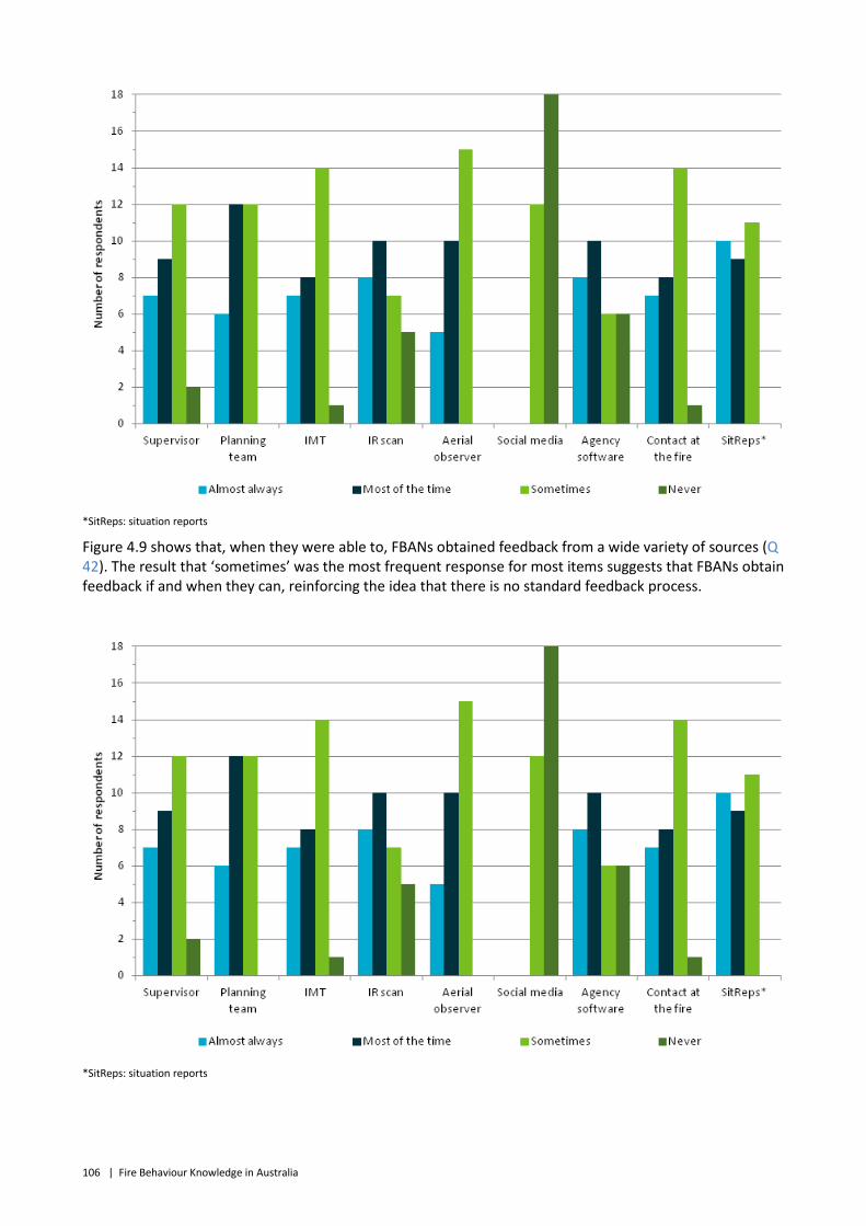
106 | Fire Behaviour Knowledge in Australia
*SitReps: situation reports
Figure 4.9 shows that, when they were able to, FBANs obtained feedback from a wide variety of sources (Q 42). The result that ‘sometimes’ was the most frequent response for most items suggests that FBANs obtain feedback if and when they can, reinforcing the idea that there is no standard feedback process.
*SitReps: situation reports
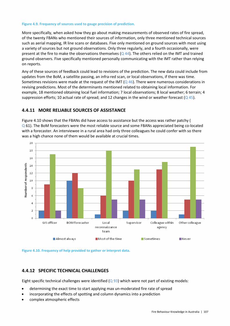
Fire Behaviour Knowledge in Australia | 107
Figure 4.9. Frequency of sources used to gauge precision of prediction.
More specifically, when asked how they go about making measurements of observed rates of fire spread, of the twenty FBANs who mentioned their sources of information, only three mentioned technical sources such as aerial mapping, IR line scans or databases. Five only mentioned on ground sources with most using a variety of sources but not ground observations. Only three regularly, and a fourth occasionally, were present at the fire to make the observations themselves (Q 44). The others relied on the IMT and trained ground observers. Five specifically mentioned personally communicating with the IMT rather than relying on reports.
Any of these sources of feedback could lead to revisions of the prediction. The new data could include from updates from the BoM, a satellite passing, an infra-red scan, or local observations, if there was time. Sometimes revisions were made at the request of the IMT (Q 46). There were numerous considerations in revising predictions. Most of the determinants mentioned related to obtaining local information. For example, 18 mentioned obtaining local fuel information; 7 local observations; 8 local weather; 6 terrain; 4 suppression efforts; 10 actual rate of spread; and 12 changes in the wind or weather forecast (Q 45).
4.4.11 MORE RELIABLE SOURCES OF ASSISTANCE
Figure 4.10 shows that the FBANs did have access to assistance but the access was rather patchy ( Q 61). The BoM forecasters were the most reliable source and some FBANs appreciated being co-located with a forecaster. An interviewee in a rural area had only three colleagues he could confer with so there was a high chance none of them would be available at crucial times.
Figure 4.10. Frequency of help provided to gather or interpret data.
4.4.12 SPECIFIC TECHNICAL CHALLENGES
Eight specific technical challenges were identified (Q 93) which were not part of existing models:
• determining the exact time to start applying max un-moderated fire rate of spread • incorporating the effects of spotting and column dynamics into a prediction • complex atmospheric effects
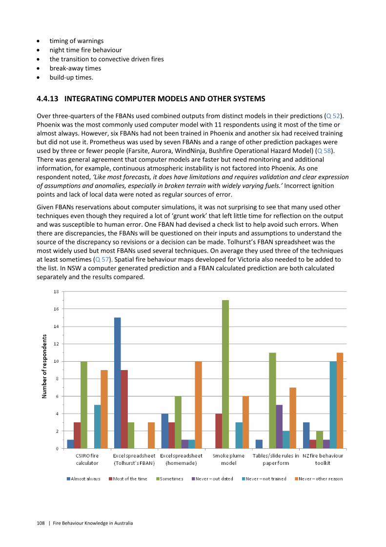
108 | Fire Behaviour Knowledge in Australia
• timing of warnings • night time fire behaviour • the transition to convective driven fires • break-away times • build-up times.
4.4.13 INTEGRATING COMPUTER MODELS AND OTHER SYSTEMS
Over three-quarters of the FBANs used combined outputs from distinct models in their predictions (Q 52). Phoenix was the most commonly used computer model with 11 respondents using it most of the time or almost always. However, six FBANs had not been trained in Phoenix and another six had received training but did not use it. Prometheus was used by seven FBANs and a range of other prediction packages were used by three or fewer people (Farsite, Aurora, WindNinja, Bushfire Operational Hazard Model) (Q 58). There was general agreement that computer models are faster but need monitoring and additional information, for example, continuous atmospheric instability is not factored into Phoenix. As one respondent noted, ‘Like most forecasts, it does have limitations and requires validation and clear expression of assumptions and anomalies, especially in broken terrain with widely varying fuels.’ Incorrect ignition points and lack of local data were noted as regular sources of error.
Given FBANs reservations about computer simulations, it was not surprising to see that many used other techniques even though they required a lot of ‘grunt work’ that left little time for reflection on the output and was susceptible to human error. One FBAN had devised a check list to help avoid such errors. When there are discrepancies, the FBANs will be questioned on their inputs and assumptions to understand the source of the discrepancy so revisions or a decision can be made. Tolhurst’s FBAN spreadsheet was the most widely used but most FBANs used several techniques. On average they used three of the techniques at least sometimes (Q 57). Spatial fire behaviour maps developed for Victoria also needed to be added to the list. In NSW a computer generated prediction and a FBAN calculated prediction are both calculated separately and the results compared.
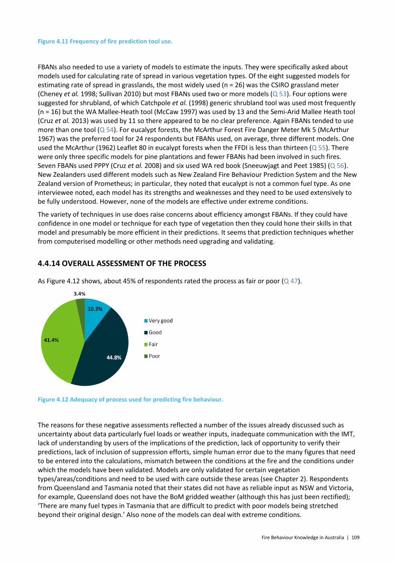
Fire Behaviour Knowledge in Australia | 109
Figure 4.11 Frequency of fire prediction tool use.
FBANs also needed to use a variety of models to estimate the inputs. They were specifically asked about models used for calculating rate of spread in various vegetation types. Of the eight suggested models for estimating rate of spread in grasslands, the most widely used (n = 26) was the CSIRO grassland meter (Cheney et al. 1998; Sullivan 2010) but most FBANs used two or more models (Q 53). Four options were suggested for shrubland, of which Catchpole et al. (1998) generic shrubland tool was used most frequently (n = 16) but the WA Mallee-Heath tool (McCaw 1997) was used by 13 and the Semi-Arid Mallee Heath tool (Cruz et al. 2013) was used by 11 so there appeared to be no clear preference. Again FBANs tended to use more than one tool (Q 54). For eucalypt forests, the McArthur Forest Fire Danger Meter Mk 5 (McArthur 1967) was the preferred tool for 24 respondents but FBANs used, on average, three different models. One used the McArthur (1962) Leaflet 80 in eucalypt forests when the FFDI is less than thirteen (Q 55). There were only three specific models for pine plantations and fewer FBANs had been involved in such fires. Seven FBANs used PPPY (Cruz et al. 2008) and six used WA red book (Sneeuwjagt and Peet 1985) (Q 56). New Zealanders used different models such as New Zealand Fire Behaviour Prediction System and the New Zealand version of Prometheus; in particular, they noted that eucalypt is not a common fuel type. As one interviewee noted, each model has its strengths and weaknesses and they need to be used extensively to be fully understood. However, none of the models are effective under extreme conditions.
The variety of techniques in use does raise concerns about efficiency amongst FBANs. If they could have confidence in one model or technique for each type of vegetation then they could hone their skills in that model and presumably be more efficient in their predictions. It seems that prediction techniques whether from computerised modelling or other methods need upgrading and validating.
4.4.14 OVERALL ASSESSMENT OF THE PROCESS
As Figure 4.12 shows, about 45% of respondents rated the process as fair or poor (Q 47).
Figure 4.12 Adequacy of process used for predicting fire behaviour.
The reasons for these negative assessments reflected a number of the issues already discussed such as uncertainty about data particularly fuel loads or weather inputs, inadequate communication with the IMT, lack of understanding by users of the implications of the prediction, lack of opportunity to verify their predictions, lack of inclusion of suppression efforts, simple human error due to the many figures that need to be entered into the calculations, mismatch between the conditions at the fire and the conditions under which the models have been validated. Models are only validated for certain vegetation types/areas/conditions and need to be used with care outside these areas (see Chapter 2). Respondents from Queensland and Tasmania noted that their states did not have as reliable input as NSW and Victoria, for example, Queensland does not have the BoM gridded weather (although this has just been rectified); ‘There are many fuel types in Tasmania that are difficult to predict with poor models being stretched beyond their original design.’ Also none of the models can deal with extreme conditions.
110 | Fire Behaviour Knowledge in Australia
4.5 Results 3: Areas of confidence
Despite the issues raised above, only two FBANs said they were not confident in the models they commonly use to predict fire behaviour (Q 51). All but three said their knowledge of the models they use was good or excellent (Q 50). Over half reported that their predictions were largely or totally accepted by the planning team or IMT (Q 49) and were also frequently used by other groups, including community warning preparation (n = 24) and public liaison groups (n = 16) (Q 39). Nearly all (n = 27) were able to make their predictions in time to be useful, at least most of the time (Q 48).
In terms of their data input, they were either confident (86%) or very confident (14%) of their air temperature inputs (Q 65) with a margin of error of 1–5 degrees (Q 66). Only two FBANs were not confident of their relative humidity inputs. Others were confident (83%) or very confident (10%) (Q 67), with less than a 10% margin of error (Q 68).
FBANs work under tight time pressures but only three said there was a problem with the timeliness of their predictions. On average, they estimated it took 54 minutes to produce a prediction for the next two hours (Q 31), 115 minutes for a prediction for the next six to nine hours (Q 32), and 192 minutes for the next 24 to 36 hours (Q 33). Weather inputs (17 minutes) and fire location and perimeter (15 minutes) were the longest tasks (Q 60).
When asked about their particular areas of confidence (Q 92), of the 26 responses, 8 listed rate of spread, 4 mentioned using the models they are familiar with, 4 mentioned predicting the initial stages and build up of the fire; 5 mentioned effects of various fuels, 2 weather, 3 topographical effects; 2 said they were confident if there was good data; 1 was confident of predicting the fire without suppression efforts; 1 communicating ease of suppression to IMTs.
4.6 Discussion
Rapid advances in fire prediction technologies have greatly increased the effectiveness and the specialisation of fire behaviour analysis. As with most times of rapid change there is a need for reflection, integration, and validation. There is also a need to adjust organisational systems, roles and training to maximise the benefits. The results showed that nearly half the FBANs in this study rated the adequacy of their prediction process as fair or poor and identified a number of areas where the role of the FBAN could be better supported. Rectifying the problems identified by the FBANs in this survey appears quite manageable and a worthwhile investment given the lives and property that are at stake.
4.6.1 MORE RELIABLE LOCAL INPUTS
Predictions would be improved with more reliable local inputs, especially for fuel–including its type, arrangements, structure, moisture, and spatial variation. The current fuel maps were not seen as being sufficiently reliable. Local wind speed and direction were also often problematic. Precipitation and atmospheric conditions were described as problematic less frequently but misjudgements of their effects can be dangerous. For example, deaths have occurred due to overestimating the effects of light rain. Measures of atmospheric conditions were considered important for predicting unstable fire behaviour with dangerous ‘blow-ups’ but the BoM are reducing the number of sites for upper air soundings, thus making these inputs to F160 aerological charts less reliable.
Those working at the district level were more familiar with the local conditions such as vegetation types and some topographical effects however only six FBANs usually had access to the fire site themselves and only one mentioned a trained ground observer. For the others, access to local data seemed to be rather ad hoc.
There were several suggested approaches to obtaining more reliable local inputs:
• One was the development of the role of ground observer in local crews or IMTs. Ground observers would make systematic observations and measurements of their district as prescribed by an FBAN at

Fire Behaviour Knowledge in Australia | 111
the beginning of the fire season and at regular intervals so that when a fire started, their data would be on a central system and the FBANs could communicate directly with them. NSW RFS is interested in this approach and currently trying to obtain funding to develop the reconnaissance role.
• Another approach is to have more FBANs at the district or regional level so that they can become very familiar with local conditions. This would require the training of more FBANs which, as noted before, requires highly technical ongoing training and a great deal of experience. Decentralising the FBAN role leads to greater specialisation but less uniformity in the FBAN skills and thus less flexibility in their deployment to fires in other regions or interstate. However, a positive of decentralised FBANs is the likelihood of easier communication with the IMT and closer consultation between the FBAN and the Planning Officer and Incident Controller and any other agencies operating in the region.
• The vegetation across Australia and New Zealand is diverse and more mapping and testing of the diverse fuel types in needed so that the models and simulations can be more accurate.
• Improved technology provides a third approach to more reliable local inputs. Portable automatic weather stations that are consistent with BoM standards cost over $20,000 but the BoM is developing a data system that can use data from less the inexpensive models ($1,000) thus allowing the potential deployment of multiple weather stations at key sites even in the path of the fire. Improved satellite coverage (such as from the new BoM multi-spectral satellite) and aerial depictions also improve the FBAN’s knowledge of vegetation, fuel, and weather.
4.6.2 IMPROVED COMMUNICATION WITH THE INCIDENT MANAGEMENT TEAM
Education of IMT leaders was seen as key for the FBANs to obtain the feedback they need and for their predictions to be properly interpreted. In some cases FBANs first presented a ‘worst case scenario’ which was rejected by the IMT due to local knowledge. When the IMT did not register that this was the worst case, not the most likely case, the FBAN could be discredited and ignored. Most FBANs wanted to move beyond the worst case scenario, but that required intelligence on the suppression efforts of the fire crews, for which they need good feedback from the IMT. It is important to note that not all IMT leaders are knowledgeable about fire behaviour: some incident controllers are only experienced in incident management.
Although it is useful for the incident controller, operations manager, and planning officer to all have some understanding of the FBAN role it would seem that the strongest communication needs to be with the planning officer, as it is the planning officer that works out the strategy and resources. One obstacle might be that FBAN outputs are quite variable, so more standardised products might be easier for educating IMT leaders. Alternatively, locating FBANs at the regional level would allow for non-standard products that are particularly tailored to the needs of local personnel.
Further, several interviewees suggested that the ideal scenario is one in which the IMT can ask specific practical questions of the FBAN, such as the time before a fire reaches a certain road or the best approach to suppression in a given context. Such exchanges require the IMTs to understand the FBANs skills and the FBANs being able to give their expert opinion in time for the planning officer to incorporate those predictions in the plans for the day.
Although very few FBANs said they had difficulty with the timeliness of their predictions, the fact that they were not in close contact with the IMT might mean that they have limited knowledge of the actual time pressures for specific information.
4.6.3 COMPLEXITY OF MANAGING INPUTS AND PREDICTIONS FROM NUMEROUS MODELS
To a certain extent, a variety of models is desirable to deal with differing local conditions and to validate predictions by comparisons across methods. Australia and New Zealand have such diverse terrains that models need to be validated in many locations. Western Australia’s vegetation is unique and more models need to be developed for their particular conditions. However, there were a very large number of models
112 | Fire Behaviour Knowledge in Australia
that FBANs used only occasionally, making it difficult for them to become expert in the strengths, weaknesses, and assumptions of them all. The FBANs work could be simplified by further development and validation of a smaller selection of models so they can be used with confidence. The work in assessing models in Chapter 2 goes some way to simplifying the selection process but it will take some time before FBANs have access to and expertise in all the recommended models.
Simulation programs, such as Phoenix, simplify the incorporation of data from many sources but they were not trusted by the FBANs who usually tried to manually verify the prediction from the simulation. Manual predictions on the other hand are relatively slow and laborious decreasing the likelihood of a timely prediction and increasing the likelihood of human error. A check-list developed by one FBAN to minimise errors, could be used more widely. To maximise speed and accuracy, one FBAN suggested a semi-automatic simulation program for which each step can be seen and monitored for reasonableness by the FBAN.
Further, some computerised simulations are not modularised so that it is not easy to update them as better models emerge or to add in more indicators (such as F160 which is missing from Phoenix). If the current programs are not revised then FBANs and their managers will have the difficult decision about if and when they move to an entirely different simulation program. Models and simulations need to be updated to deal with the extreme conditions which will be more prevalent with climate change.
4.6.4 FURTHER TRAINING
Although all the FBANs used a range of informal systems for updating their skills (e.g. reading case studies, reading research publications, and online groups) and these could be developed with mechanisms to share the latest science and other developments. However, there was a need for more formal courses to increase their skills and keep them up to date with technical developments. Indeed if regular courses were available on the new models and computer simulations, then the problem mentioned above about the complexity of inputs from numerous models and learning about new computer simulations would be minimised.
There will be an ongoing tension between the need for uniform training and training for specific conditions experienced in the diverse locations across Australia and New Zealand but clearly both need to be addressed. FBANs might also benefit from training in decision-making with insufficient data. Uncertainty will often be present due to the wide array of data that is needed for precise prediction, but there are risk assessment and decision-making models that might be useful.
The issue of increased training to up-skill the level of the FBAN workforce needs to be distinguished from the other role of training, which is accreditation. Accreditation requires designated standards, assessment, and registration and is probably best managed through an existing tertiary institution. There is a national training module but only one person has completed it. One obstacle is lack of a process for assessment of the portfolios for the module.
The benefits of professionalisation would be public recognition of FBANs’ expertise, transportability of their qualifications, and uniformity of training standards. The negatives of such courses for FBANs would be the increased cost and time invested at the early training stage, when their main concerns were about updating their skills and gaining practical experience. A challenge will be to address both universal and local knowledge otherwise local knowledge and respect for that knowledge is likely to dwindle.
There is a clear role for the Australasian Fire and Emergency Service Authorities Council (AFAC) in managing the accreditation processes.
4.6.5 A NEED FOR MORE OPPORTUNITIES TO GAIN EXPERIENCE AND FEEDBACK
Because the FBANs believed that experience was a major contributor to their predictions, opportunities to both practice their skills and to gain feedback are essential. This was a challenge for the many part-time FBANs, especially those whose regular jobs are not fire related. Some FBANs lacked regular assignments partly because extra FBANs are called in when the regulars are too busy and that is when the fire situation is severe. This creates an inverse relationship between the size of the fire problem and experience of FBANs

Fire Behaviour Knowledge in Australia | 113
which does not seem ideal. Thus, regular rostering of FBANs and establishing mentoring programs would be valuable.
More significantly, there was a general lack of regular feedback on their predictions suggesting the need for feedback systems to be put in place. The range of inputs FBANs used to try to validate their predictions shows that they were making an effort but that there were no particular systems in place. Indeed the identification of fuel and wind inputs as the most common sources of error could be questioned because FBANs have so few opportunities to validate their predictions.
Access to aerial infra-red line scans of the fire front were identified as useful feedback mechanisms and some fire authorities are increasing the number of scans to four per day. The use of drones is being explored for increasing the number of scans in the future. However, one interviewee who had a good knowledge of his local conditions was still unable to make any of the models or simulations fit the actual rate of spread.
Furthermore, validation needs to address more than the rate of spread, thus even more detailed data is needed such as the actual weather conditions at the fire site suggesting another important activity for the field observer role. Thus, further detailed study would be needed to identify the cause of any discrepancy between the actual and predicted rate of spread.
4.6.6 ACCESSING ONLINE SYSTEMS AND DATABASES
Administrative arrangements need to be put in place to enable FBANs from a variety of agencies to travel interstate to work on a severe fire situation. All the FBANs will need suitable equipment, access to any central databases, and understanding of the fire authority systems. So standardised, quick basic training systems need to be put in place. Even regular FBANs appreciated pre-season updates to familiarise themselves with any new systems and models.
FBANs in regional areas need to be properly resourced so they are not dependent on web access which may not be reliable. Although such adjustments seem straight forward, organising systems across government departments can be difficult to negotiate and some states have had more success than others.
4.7 Concluding remarks
Rapid advances in fire prediction technologies have greatly increased the effectiveness and the specialisation of fire behaviour analysis. As with most times of rapid change there is a need for reflection, integration, and validation. There is also a need to adjust organisational systems, roles and training to maximise the benefits. Rectifying the problems identified by this study appears quite manageable and a worthwhile investment given the lives and property that are at stake.

114 | Fire Behaviour Knowledge in Australia
5 References
Achtemeier, G.L. 2013. Field validation of a free-agent cellular automata model of fire spread with fire-atmosphere coupling. International Journal of Wildland Fire 22, 148-156.
AFAC 2012. Bushfire Glossary. Prepared by Rural and Land Management Group for AFAC agencies. AFAC, Melbourne, 30 pp.
Albini, F.A. 1976. Estimating wildland fire behavior and effects. USDA Forest Service, Intermountain Forest and Range Experiment Station, Ogden, Utah. General Technical Report INT-130. 92 p.
Albini FA. 1979. Spot fire distance from burning trees–a predictive model. General Technical Report INT-56, USDA Forest Service, Intermountain Forest and Range Experimental Station, Odgen UT.
Albini, F.A.; Alexander, M.E.; Cruz, M.G. 2012. A mathematical model for predicting the maximum potential spotting distance from a crown fire. International Journal of Wildland Fire 21, 609-627.
Albini, F.A. and Reinhardt, E.D. 1995. Modeling ignition and burning rate of large woody natural fuels. International Journal of Wildland Fire 5, 81-91.
Alexander, M.E. 1985. Estimating the length-to-breadth ratio of elliptical forest fire patterns. Pages 287-304 in Proc. Eighth Conf. Fire and For. Meteorol. (Apr. 29-May 2, 1985, Detroit, MI). Soc. Amer. For., Bethesda, MD. SAF Publ., 85-04
Alexander, M.E. 1998. Crown fire thresholds in exotic pine plantations of Australasia. Australian National University, Canberra, Australian Capital Territory. Ph.D. Thesis 228 p. >Alexander, M.E. 2009. Are we abusing our use of models and modelling in wildland fire and fuel management? Fire Management Today 69(4): 24-27.
Alexander, M.E.; Cruz, M.G. 2006. Evaluating a model for predicting active crown fire rate of spread using wildfire observations. Canadian Journal of Forest Research 36: 3015-3028.
Alexander ME, Cruz MG. 2013a. Assessing the effect of foliar moisture on the spread rate of crown fires. International Journal of Wildland Fire 22, 415–427.
Alexander, M.E.; Cruz, M.G. 2013b. Limitations on the accuracy of model predictions of wildland fire behaviour: a state-of-the-knowledge overview. Forestry Chronicle 89: 370-381.
Alexander, M.E.; Cruz, M.G. 2013c. Are the applications of wildland fire behaviour models getting ahead of their evaluation again? Environmental Modelling & Software 41, 65-71.
Alexander, M.E., Thomas, D.A., 2004. Forecasting wildland fire behavior: Aids and guides, and knowledge-based protocols. Fire Management Today 64, 4-11.
Allen, A. 2013. Aurora: National Bushfire Detection, Prediction, Simulation and Early Warning System. Talk presented at the CSIRO Bushfire Science Symposium, Canberra October 14-16 2013.
Anderson D.H., Catchpole E.A., de Mestre N.J., Parkes T. 1982. Modelling the spread of grass fires. Journal of Australian Mathematics Society 23, 451-466.
Andrews PL. 2014. Current status and future needs of the BehavePlus Fire Modeling System. International Journal of Wildland Fire 23, 21–33.
Balbi, J., Morandini, F., Silvani, X., Filippi, J. and Rinieri, F. 2009. A physical model for wildland fires. Combustion and Flame 156, 2217-2230.
Barrows, J.S. 1951. Fire behavior in northern Rocky Mountain forests. USDA Forest Service, Northern Rocky Mountain Forest and Range Experiment Station, Missoula, Montana. Station Paper No. 29. 103 p. + Appendices.

Fire Behaviour Knowledge in Australia | 115
Batchelor G. 1967. An Introduction to Fluid Mechanics. Cambridge University Press, London.
Beck, J.A. 1995. Equations for the Forest Fire Behaviour Tables for Western Australia. CALM Science 1, 325-348.
Bose, C., Bryce, R. and Dueck, G. 2009. Untangling the Prometheus Nightmare. In: Anderssen, R. S.; Braddock, R. D. & Newham, L. T. H. (Eds.) 18th World IMACS Congress and MODSIM09 International Congress on Modelling and Simulation, 13-17 July 2009, Cairns, Australia. 240-246.
Bradstock R.A., Gill, A.M. 1993. Fire in semi-arid Mallee shrublands: size of flames from discrete fuel arrays and their role in the spread of fire. Int. J. Wildland Fire 3:3-12.
Buckley, A.J. 1993. Fuel reducing regrowth forests with a wiregrass fuel type: fire behaviour guide and prescriptions. Research Report No. 40. Department of Conservation and Natural Resources, Fire Management Branch, East Melbourne, VIC.
Burrows, N.D. 1984. Predicting blow-up fires in the jarrah forest. Forests Department, Perth, Western Australia. Technical Paper No. 12 27 p.
Burrows, N.; Ward, B.; Robinson, A. 1988. Aspects of fire behaviour and fire suppression in a Pinus radiata plantation. Western Australia Department of Conservation and Land Management, Perth, Western Australia. Landnote 2/88. 4 p.
Burrows, N., Ward, B. and Robinson, A. 1991. Fire behaviour in spinifex fuels on the Gibson Desert Nature Reserve, Western Australia. Journal of Arid Environments 20, 189-204.
Burrows, N.D. 1994. Experimental development of a fire management model for jarrah (Eucalyptus marginata Donn ex Sm.) forest. Aust. Natl. Univ., Canberra, Australian Capital Territory,. Ph.D. thesis. 293 pp.
Burrows, N.D. 1999. Fire behaviour in jarrah forest fuels: 2. field experiments. CALM Science 3, 57-84.
Burrows, N.D., 1999. Fire behaviour in jarrah forest fuels: 2. Field experiments. CALMScience 3, 57–84.
Burrows, N.D., Sneeuwjagt, R.J. 1991. McArthur’s forest fire danger meter and the forest fire behaviour tables for western Australia: derivation, application and limitations. In: Cheney, N. P; Gill, A. M., (Eds), Proceedings Of Conference On Bushfire Modeling And Fire Danger Rating Systems; 11–12 July 1988; Canberra, ACT: CSIRO Division of Forestry, 65-77.
Burrows, N.D.; Ward, B.; Robinson, A. 2000. Behaviour and some impacts of a large wildfire in the Gnangara martime pine (Pinus pinaster) plantation, Western Australia. CALMscience 3: 251-260.
Burrows, ND, Ward B, Robinson A (2009) Fuel dynamics and fire spread in spinifex grasslands of the western desert. In Tran, C. (Ed.) The Proceedings of the Royal Society of Queensland – Bushfire 2006 conference. Brisbane 6-9 June 2006, 69-76.
Byram, G.M. 1959. Combustion of forest fuels. Pages 61-89 in K.P. Davis (ed.). Forest Fire: Control and Use. McGraw Hill, New York
Byrne, P.J. 1980. Prescribed burning in Queensland exotic pine plantations. Queensland Department of Forestry, Brisbane, Queensland. Paper prepared for the Eleventh Commonwealth Forestry Conference. 58 p.
Canadian Wildland Fire Growth Model. 2009. Prometheus the Canadian Wildland Fire Growth Simulation Model, 5.2.2 User Manual (May 4, 2009). 225 pp.
Catchpole, T.; de Mestre, N. 1986. Physical models for a spreading line fire. Australian Forestry 49: 101-111.
Catchpole, W.R., Bradstock, R.A., Choate, J., Fogarty, L.G., Gellie, N., McCarthy, G., McCaw, W.L., Marsden-Smedley, J.B., Pearce, G. 1998 Cooperative development of equations for heathland fire behaviour. In ‘III International Conference on Forest Fire Research/14th Conference on Fire and Forest Meteorology Proceedings, Volume II’, 16-20 November 1998, Luso, Portugal. (DX Viegas, Ed.) pp. 631-645. (ADAI, University of Coimbra: Coimbra, Portugal).

116 | Fire Behaviour Knowledge in Australia
Catchpole, W. 2002. Fire properties and burn patterns in heterogeneous landscapes. Pages 49-75 in R.A. Bradstock, J.E. Williams and A.M. Gill (eds.), Flammable Australia: The Fire Regimes and Biodiversity of a Continent. University Press, Cambridge, UK.
Chandler, C.C.; Countryman, C.M. 1959. Use of fire behavior specialists can pay off. Fire Control Notes 20, 130-132.
Cheney, N.P. 1968. Predicting fire behaviour with fire danger tables. Australian Forestry 32:71-79.
Cheney, N.P. 1981. Fire behaviour. Pages 151-175 in A.M. Gill, R.H.Groves and I.R. Noble (eds.). Fire and the Australian Biota. Australian Academy of Science, Canberra, Australian Capital Territory.
Cheney, N.P. 1991. Models used for fire danger rating in Australia. In: Cheney, N. P; Gill, A. M., (Eds), Proceedings of Conference on Bushfire Modelling and Fire Danger Rating Systems, 11-12 July 1988, Canberra, ACT, CSIRO Division of Forestry, 19-28.
Cheney, N.P.; Bary, G.A.V. 1969. The propagation of mass conflagrations in a standing eucalypt forest by the spotting process. Paper A6 in Collected Papers, Mass Fire Symposium, Volume I. Commonwealth of Australia, Defence Standards Laboratory, Maribyrnong, Victoria. 18 p.
Cheney, N.P., 1968. Predicting fire behaviour with fire danger tables. Australian Forestry 32, 71-79, DOI: 10.1080/00049158.1968.10675463.
Cheney, N.P. 1981. Fire behaviour. Pages 151-175 in A.M. Gill, R.H. Groves and I.R. Noble (eds.). Fire and the Australian Biota. Australian Academy of Science, Canberra, Australian Capital Territory.
Cheney N.P. and Gould, J.S. (1996) Development of fire behaviour models for high-intensity forest fires. NDR96 Conference on Natural Disaster Reduction. 29 September – 2 October 1996. Gold Coast. Australia.
Cheney, N.P., Gould, J.S., and Catchpole, W.R. 1993. The influence of fuel, weather and fire shape variables on fire-spread in grasslands. International Journal of Wildland Fire 3, 31-44.
Cheney, N.P., Gould, J.S., Catchpole, W.R. 1998. Prediction of fire spread in grasslands. International Journal of Wildland Fire 8(1):1-15.
Cheney, N.P., Gould, J.S., Knight, I., 1992. A prescribed burning guide for young regrowth forest of silvertop ash. Forestry Commission of NSW Research Report No. 16. 91 pp.
Cheney, N.P., Gould, J.S., McCaw, L., 1998. Project Vesta: Research initiative into the effects of fuel structure and fuel load on behaviour of wildfires in dry eucalypt forest. In: Proceedings 13th International Conference of Forest Fire and Meteorology. International Association of Wildland Fire, pp. 375 – 78.
Cheney, N.P., Gould, J.S. McCaw, W.L. Anderson, W.R., 2012. Predicting fire behaviour in dry eucalypt forest in southern Australia. Forest Ecology and Management. 280, 120-131. doi: 10.1016/foreco.2012.06.012
Cheney, N.P., Just, T.E. (1974). The behaviour and application of fire in sugar cane in Queensland. Leaflet No. 115. Australian Department of Agriculture, Forestry and Timber Bureau, Canberra, ACT.
Cheney, P., Sullivan, A. 2008. Grassfires: Fuel, Weather and Fire Behaviour. Second edition. CSIRO Publishing, Collingwood, Australia. 160 pp.
Chong, D. M. and Tohurst, K. 2012. Phoenix- Under the Hood. A Technical guide to the Phoenix bushfire Characterisation Model, Version 3.9. University of Melbourne, 27 pp.
Chong, D., Tolhurst, K. and Duff, T. 2012a. PHOENIX Rapidfire 4.0's Convective Plume Model. Bushfire CRC, 23 pp.
Chong, D., Tolhurst, K. and Duff, T. 2012b. PHOENIX Rapidfire 4.0's Convection and Ember Dispersal Model. Bushfire CRC, 22 pp.
Fire Behaviour Knowledge in Australia | 117
Chong, D., Tolhurst, K., Duff, T. and Cirulis, B. 2013. Sensitivity analysis of PHOENIX Rapidfire. Bushfire CRC, 27 pp.
Clark, T.L., Coen, J. and Latham, D. 2004. Description of a coupled atmosphere-fire model. International Journal of Wildland Fire 13, 49-63.
Clark, T., Coen, J., Radke, L., Reeder, M. and Packham, D. 1998. Coupled atmosphere-fire dynamics. III International Conference on Forest Fire Research. 14th Conference on Fire and Forest Meteorology Luso, Portugal, 16-20 November 1998. Vol 1, 67-82
Coen, J.L. 2005. Simulation of the Big Elk Fire using coupled atmosphere/fire modeling. International Journal of Wildland Fire 14, 49-59.
Coen, J.L. and Clark, T.L. 2000. Coupled atmosphere-fire model dynamics of a fireline crossing a hill. Third Symposium on Fire and Forest Meteorology, 9-14 January 2000, Long Beach, California. 7-10.
Coleman, J.R., Sullivan, A.L. 1995. SiroFire: the CSIRO bushfire spread simulator. In: Proc. Inst. Foresters Aust. 16th Biennial Conf. Canberra, 309-319.
Coleman, J.R., Sullivan, A.L. 1996. A real-time computer application for the prediction of fire spread across the Australian landscape. Simulation 67, 230-240.
Colman, J.J. and Linn, R.R. 2003. Non-local chemistry implementation in HIGRAD/FIRETEC. Fifth Symposium on Fire and Forest Meteorology, 16-20 November 2003, Orlando, Florida.
Colman, J. J. and Linn, R. R. 2007. Separating combustion from pyrolysis in HIGRAD/FIRETEC. International Journal of Wildland Fire 16, 493-502
Commonwealth of Australia 2008. Australia’s State of the Forests Report 2008. Bureau of Rural Sciences, Canberra.
Cook, B., Price, O., Chong, D. and Tolhurst, K. 2009. Review of Potential Applications for Bushfire Behaviour Models for Bushfire Management in NSW. Final Report to NSW Rural Fire Service. University of Wollongong and University of Melbourne, 68 pp.
Countryman, C.M.; Chandler, C.C. 1963. The fire behavior team approach in fire control. Fire Control Notes 24, 56-60.
Crane, W.B. 1982. Computing grassland and forest fire behaviour, relative humidity and drought index by pocket calculator. Australian Forestry 45: 89-97.
Cruz, M.G.; Alexander, M.E. 2013. Uncertainty associated with model predictions of surface and crown fire rates of spread. Environmental Modelling & Software 47, 16-28.
Cruz, M.G., Alexander, M.E., Fernandes, P. 2008. Development of a model system to predict wildfire behaviour in pine plantations. Australian Forestry 71, 113-121.
Cruz, M.G., Alexander, M.E., Wakimoto, R.H. 2004. Modeling the likelihood of crown fire occurrence in conifer forest stands. Forest Science 50: 640-658.
Cruz, M.G., Alexander, M.E., Wakimoto, R.H. 2005. Development and testing of models for predicting crown fire rate of spread in conifer forest stands. Canadian Journal of Forest Research 35: 1626-1639.
Cruz, M.G.; Butler, B.W.; Alexander, M.E. 2006a. Predicting the ignition of crown fuels above a spreading surface fire. Part II: Model behavior and evaluation. International Journal of Wildland Fire 15: 61-72.
Cruz, M.G.; Butler, B.W.; Alexander, M.E.; Forthofer, J.M.; Wakimoto, R.H. 2006b. Predicting the ignition of crown fuels above a spreading surface fire. Part I: Model idealization. International Journal of Wildland Fire 15: 47-60.
Cruz, M.G. and Fernandes, P.A.M. (2008) Development of fuel models for fire behaviour prediction in maritime pine (Pinus pinaster Ait.) stands. International Journal of Wildland Fire 17,194-204.
118 | Fire Behaviour Knowledge in Australia
Cruz, M.G., Gould, J 2009a. Field-based fire behaviour research: past and future roles. Proceedings of the 18th World IMACS / MODSIM congress, Cairns, Australia 13-17 July 2009, 247-253.
Cruz, M.G.; Gould, J. 2009b. National fire behaviour prediction system. Pages 285-291 in Proceedings of the Biennial Conference of the Institute of Foresters of Australia. Institute of Foresters of Australia, Yarralumla, Australian Capital Territory.
Cruz, M.G., Matthews, S., Gould, J., Ellis, P. Henderson, M. Knight, I., Watters, J. 2010. Fire dynamics in mallee-heath: fuel, weather and fire behaviour prediction in south Australian semi-arid shrublands. Bushfire CRC report A.10.01.
Cruz, M.G., McCaw, W.L., Anderson, W.R., Gould, J.S. 2013. Fire behaviour modelling in semi-arid mallee-heath shrublands of southern Australia, Environmental Modelling and Software, 40:21-34.
Cruz, M.G.; Plucinski, M.P. 2007. Billo Road Fire – report on fire behaviour phenomena and suppression activities. Bushfire Cooperative Research Centre, East Melbourne, Victoria. Report No. A.07.02. 96 p.
Cruz M.G., Sullivan AL, Gould JS, Sims NC, Bannister AJ, Hollis JJ, Hurley RJ. 2012. Anatomy of a catastrophic wildfire: The Black Saturday Kilmore East fire in Victoria, Australia. Forest Ecology and Management 284, 269-285.
Cunningham, P., Goodrick, S. L., Hussaini, M. Y. and Linn, R. R. 2005. Coherent vortical structures in numerical simulations of buoyant plumes from wildland fires. International Journal of Wildland Fire 14, 61-75.
Davis KM (1976) Behaviour and effects of fire during mild weather. Devision of Forest Research Internal Report 3. CSIRO, Canberra, Australia. 7 pp.
Dell, J.D. 1966. The fire-behavior team in action - the Coyote Fire. Fire Control Notes 27(1), 8-10, 15.
Demeritt, D., Cloke, H., Pappenberger, F., Thielen, J., Bartholmes, J., & Ramos, M. (2007). Ensemble predictions and perceptions of risk, uncertainty, and error in flood forecasting. Environmental Hazards 7(2), 115-127. doi: 10.1016/j.envhaz.2007.05.001
DEH, 2006. Overall fuel hazard guide for South Australia. Department of Environment and Heritage. Adelaide, SA.
Drysdale D. 1985. An Introduction to Fire Dynamics. John Wiley and Sons, Chichester.
Duff, T. J., Chong, D. M. and Tolhurst, K. G. 2013. Quantifying spatio-temporal differences between fire shapes: Estimating fire travel paths for the improvement of dynamic spread models. Environmental Modelling & Software 46, 33-43.
Duff, T. J., Chong, D. M., Taylor, P. and Tolhurst, K. G. 2012. Procrustes based metrics for spatial validation and calibration of two-dimensional perimeter spread models: A case study considering fire. Agricultural and Forest Meteorology 160, 110-117.
Duff, T.J., Chong, D.M., and Tolhurst, K.G. In review. The Area Difference Index (ADI), an improved index for the comparison of patterns of fire spread. Submitted to the Journal of Environmental Informatics.
Ellis PFM. 2000. The aerodynamic and combustion characteristics of eucalypt bark: A firebrand study. PhD thesis, The Australian National University School of Forestry, Canberra.
Ellis PFM. 2011. Fuelbed ignition potential and bark morphology explain the notoriety of the eucalypt messmate `stringybark' for intense spotting. International Journal of Wildland Fire 20, 897-907.
Ellis PFM. 2013. Firebrand characteristics of the stringy bark of messmate (Eucalyptus obliqua) investigated using non-tethered samples. International Journal of Wildland Fire 22, 642-651.
Emmons, H. 1966. Fundamental problems of the free burning fire. Fire Research Abstracts and Reviews 8, 1–17.
Fire Behaviour Knowledge in Australia | 119
Encinas, L.H., White, S.H., del Ray, A.M., Sanchez, G.R. 2007. Modelling forest fire spread using hexagonal cellular automata. Applied Mathematical Modelling 31, 1213-1227.
Evans, D. D., Rehm, R. G. and McPherson, E. G. 2003. Physics-based modelling of wildland-urban intermix fires. Proceedings of the 3rd International Wildland Fire Conference, 3-6 October 2003, Sydney.
Fendell, F. E. and Wolff, M. F. 2001. Wind-Aided Fire Spread. 6. In: Johnson, E. & Miyanishi, K. (Eds.) Forest Fires: Behaviour and Ecological Effects, Academic Press, 171-223.
Fernandes, P.A.M.; Loureiro, C.; Botelho, H.S. 2014. Fire behaviour and severity in a maritime pine stand under differing fuel conditions. Annals of Forest Science 61: 537-544.
Filippi, J.B., Mallet, V. and Nader, B. 2014. Representation and evaluation of wildfire propagation simulations. International Journal of Wildland Fire 23, 46-57.
Filippi, J.B., Morandini, F., Balbi, J.H. 2010. Discrete Event Front tracking: Simulation of a Physical Fire-spread Model. Simulation 86, 629-644
Finkele, K., Mills, G. A., Beard, G. and Jones, D. A. 2006. National gridded drought factors and comparison of two soil moisture deficit formulations used in prediction of Forest Fire Danger Index in Australia. Australian Meteorological Magazine 55, 183-197.
Finney, M.A. 1994. Modeling the spread and behavior of prescribed natural fires. Proc. 12th Conf. Fire and Forest Meteorology, 138-143.
Finney, M. A. 1998. FARSITE: Fire area simulator--model development and evaluation. USDA Forest Service Research Paper RMRS-RP-4, 47 pp.
Finney, M.A. 2004. FARSITE: Fire area simulator—model development and evaluation. US Department of Agriculture, Forest Service, Rocky Mountain Research Station, Research Paper RMRS-RP-4 revised, Fort Collins, CO. 47 p
Fogarty, L.G.; Jackson, A.F.; Lindsay, W.T. 1996. Fire behaviour, suppression and lessons from the Berwick Forest Fire of 26 February 1995. New Zealand Forest Research Institute, Rotorua, in association with the National Rural Fire Authority, Wellington, New Zealand. Forest Research Bulletin No. 197, Forest and Rural Fire Scientific and Technical Series Report No. 3. 38 p. + Appendices.
Foley, J.C. 1947. A study of meteorological conditions associated with bush and grass fires and fire protection strategy in Australia. Australia Bureau of Meteorology, Melbourne, Victoria. Bulletin No. 38. 234 p.
Forest and Timber Bureau. 1960. Annual report of the Forestry and Timber Bureau. Forestry and Timber Bureau, Canberra, Australia.
Forest and Timber Bureau 1970 Annual report of the Forestry and Timber Bureau. Forestry and Timber Bureau, Canberra, Australia.
Forestry Canada Fire Danger Group. 1992. Development and structure of the Canadian Forest Fire Behavior Prediction System. Forestry Canada, Science. and Sustainable Development Directorate, Ottawa, Ontario. Information Report ST-X-3. 63 p.
Forthofer, J., Butler, B. and Wagenbrenner, N. In press. A comparison of three approaches for simulating fine-scale winds in support of wildland fire management: Part I : model formulation and comparison against measurements. International Journal of Wildland Fire
French, I. A., Anderson, D. H. and Catchpole, E. A. 1990. Graphical simulation of bushfire spread. Mathematical and Computer Modelling 13, 67-71.
Gaydon, A. and Wolfhard, H. 1960. Flames: Their Structure, Radiation and Temperature. 2nd edition. Chapman and Hall Ltd, London.
Gibos, K. (2013a). Bushfire Behaviour Predictive Services Strategy: History and background of fire behaviour analysis in Victoria. Myrtleford Vic: Ovens ICC.
120 | Fire Behaviour Knowledge in Australia
Gibos, K. (2013b). Victorian Bushfire Predictive Services Strategy: Discussion Paper. Myrtleford, VIC: CFA; Ovens ICC.
Gibos, K. (2013c). Victorian Bushfire Predictive Services Strategy: Initial Stakeholder Analysis Report. Myrtleford, Vic: CFA; Ovens ICC.
Gill, A.M., Burrows, N.D. and Bradstock, R.A. 1995. Fire modelling and fire weather in an Australian desert. CALMScience Supplement 4, 29-34.
Goldstein, R. J., Ibele, W. E., Patankar, S. V., Simon, T. W., Kuehn, T. H., Strykowski, P. J., Tamma, K. K., Heberlein, J. V. R., Davidson, J. H., Bischof, J., Kulacki, F. A., Kortshagen, U., Garrick, S., and Srinivasan, V. 2006. Heat transfer: A review of 2003 literature. International Journal of Heat and Mass Transfer 49, 451–534.
Gould, J.S., 1994. Evaluation of McArthur’s control burning guide in regrowth Eucalyptus sieberia fores. Australian Forestry, 57, 86-93.
Gould, J.S., McCaw, W.L., Cheney, N.P., Ellis, P.E., Knight, I.K., Sullivan, A.L., 2007a. Project Vesta. Fire in Dry Eucalypt Forest: Fuel Structure, Fuel Dynamics, and Fire Behaviour. Ensis-CSIRO, Canberra, ACT and Department of Environment and Conservation, Perth, WA, Australia.
Gould, J.S.; McCaw, W.L.; Cheney, N.P.; Ellis, P.F.; Matthews, S. 2007b. Field guide: Fuel assessment and fire behaviour prediction in dry eucalypt forest. Interim ed. 2007. CSIRO Publishing, Collingwood, Victoria. 92 p.
Green, D.G., Gill, A.M. and Noble, I.R. 1983. Fire shapes and the adequacy of fire-spread models. Ecological Modelling 20, 33-45.
Green, D.G., Tridgell, A., Gill, A.M. 1990. Interactive simulation of bushfires in heterogeneous fuels. Mathematical and Computer Modelling 13, 57-66.
Griffin, G.F. and Allan, G.E. (1984) Fire behaviour. In Anticipating the inevitable: a patch burn strategy for fire management at Uluru (Ayers Rock-Mt Olga) National Park, Saxon, E. (Ed.), CSIRO Australia, Melbourne, 55-68
Griffiths, D., 1999. Improved formula for the drought factor in McArthur’s Forest Fire Danger Meter. Australian Forestry, 62, 202-206, doi: 10.1080/00049158.1999.10674783.
Grishin, A. 1984. Steady-state propagation of the front of a high-level forest fire. Soviet Physics Doklady 29, 917–919.
Grishin, A. 1997. Mathematical modeling of forest fires and new methods of fighting them. Publishing House of Tomsk State University, Tomsk, Russia, english translation edition. Translated from Russian by Marek Czuma, L Chikina and L Smokotina.
Handmer, J., & Proudley, B. (2007). Communicating uncertainty via probabilities: The case of weather forecasts. Environmental Hazards, 7(2), 79-87. doi: 10.1016/j.envhaz.2007.05.002
Harris, A. C., 1968. Forest fire danger tables. Forests Department Western Australia, Perth.
Hines, F., Tolhurst, K.G., Wilson, A.A.G., McCarthy, G.J., 2010. Overall Fuel Hazard Aassessment Guide, fourth edition. Department of Sustainability and Environment. Melbourne, Victoria.
Hollis, JJ, Gould, JS, Cruz MG, McCaw WL Framework for an Australian Fuel Classification to support wildland fire management. Submitted to Australian Forestry.
Hough, W.A.; Albini, F.A. 1978. Predicting fire behaviour in palmetto-gallberry fuel complexes. USDA Forest Service, Southeastern Forest Experiment Station, Asheville, North Carolina. Research Paper SE-174. 49 p.
Hunt, S.M.; Crock, M.J. 1987. Fire behaviour modelling in exotic pine plantations: testing the Queensland Department of Forestry ‘Prescribed Burning Guide Mk III’. Australian Forest Research 17: 179-189.

Fire Behaviour Knowledge in Australia | 121
Just, T.E. 1972. Prescribed burning in slash pine plantations. Queensland Department of Forestry, Brisbane, Queensland. Department Notes 2: 29-30.
Johnston, P., Kelso, J. and Milne, G. J. 2008. Efficient simulation of wildfire spread on an irregular grid. International Journal of Wildland Fire 17, 614–627.
Keetch, J.J., Byram, G.M., 1968. A drought index for forest fire control. United States Department of Agriculture, Forest Service, Southeast Forest Experiment Station, Asheville, North Carolina. Research Paper SE-38. 32 p. [revised November 1988.]
Kelso J, Mellor D and Milne G. 2011. The AUSTRALIS Wildfire Simulator. Presentation found at http://smr.csse.uwa.edu.au/pdf/Bushfire Presentation Web Site.pdf, accessed May 29 2014.
Kilinc M, Anderson W, Price B. In press. Testing the performance of fire spread models for grassland and forest in Australia. International Journal of Wildland Fire.
Knight, I., Coleman J. 1993. A fire perimeter expansion algorithm based on Huygens wavelet propagation. International Journal of Wildland Fire 3, 73-84.
Knutson, K.K. 1962. The place of the fire behavior officer in the fire suppression organization. Fire Control Notes 23, 81-82.
Kochanski, A. K., Jenkins, M. A., Mandel, J., Beezley, J. D., Clements, C. B., Krueger, S. 2013a. Evaluation of WRF-SFIRE performance with field observations from the FireFlux experiment. Geoscientific Model Development 6, 1109-1126.
Kochanski, A. K., Jenkins, M. A., Mandel, J., Beezley, J. D., Krueger, S. 2013b. Real time simulation of 2007 Santa Ana fires. Forest Ecology and Management 294, 136-149.
Lacy, P. (2009). Burning under young eucalypts: A guide for prescribed burning and post-burn assessment. Bushfire Cooperative Research Centre, Melbourne, VIC.
Linn, R.R. 1997. A Transport Model for Prediction of Wildfire Behaviour. Los Alamos National Laboratory Report LA-13334-T, PhD Thesis (New Mexico State University).
Linn, R.R. and Harlow, F.H. 1998a. FIRETEC: A transport description of wildfire behaviour. Second Symposium on Fire and Forest Meteorology, 11-16 January 1998, Pheonix, Arizona 14-19.
Linn, R.R. and Harlow, F.H. 1998b. Use of transport models for wildfire behaviour simulations. III International Conference on Forest Fire Research, 14th Conference on Fire and Forest Meteorology, Luso, Portugal, 16-20 November 1998. Vol 1, 363-372.
Linn, R., Reisner, J., Colman, J. and Smith, S. 2001. Studying wildfire behaviour using FIRETEC. Fourth Symposium on Fire and Forest Meteorology, 13-15 November 2001, Reno, Nevada. 51-55.
Linn, R., Reisner, J., Colman, J. J. and Winterkamp, J. 2002. Studying wildfire behavior using FIRETEC. International Journal of Wildland Fire 11, 233-246.
Linn, R., Winterkamp, J., Edminster, C., Colman, J. and Steinzig, M. 2003. Modeling interactions between fire and atmosphere in discrete element fuel beds. Fifth Symposium on Fire and Forest Meteorology, 16-20 November 2003, Orlando, Florida.
Linn, R., Winterkamp, J., Colman, J., Edminster, C. and Bailey, J. D. 2005. Modeling interactions between fire and atmosphere in discrete element fuel beds. International Journal of Wildland Fire 14, 37-48.
Lopes, A.M.G., Cruz,. M.G., Viegas, D.X. 2002. FireStation an integrated software system for the numerical simulation of fire spread on complex topography. Environmental Modelling and Software 17, 269-285.
Luke, R.H. and McArthur, A.G. 1978. Bushfires in Australia. Australian Government Publishing Service, Canberra. 359 pp.
Mandel, J., Beezley, J. D., Coen, J. L., and Kim, M. 2009. Data assimilation for wildland fires: ensemble Kalman filters in coupled atmosphere-surface models, IEEE Contr. Syst. Mag. 29, 47–65.
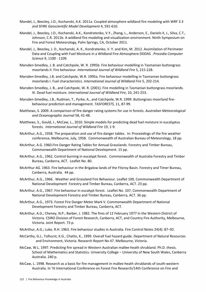
122 | Fire Behaviour Knowledge in Australia
Mandel, J., Beezley, J.D., Kochanski, A.K. 2011a. Coupled atmosphere wildland fire modeling with WRF 3.3 and SFIRE Geoscientific Model Development 4, 591-610.
Mandel, J., Beezley, J.D., Kochanski, A.K., Kondratenko, V.Y., Zhang, L., Anderson, E., Daniels II, J., Silva, C.T., Johnson, C.R. 2011b. A wildland fire modeling and visualization environment. Ninth Symposium on Fire and Forest Meteorology, Palm Springs, CA, October 2011.
Mandel, J., Beezley, J. D., Kochanski, A. K., Kondratenko, V. Y. and Kim, M. 2012. Assimilation of Perimeter Data and Coupling with Fuel Moisture in a Wildland Fire-Atmosphere DDDAS . Procedia Computer Science 9, 1100 - 1109.
Marsden-Smedley, J. B. and Catchpole, W. R. 1995b. Fire behaviour modelling in Tasmanian buttongrass moorlands II. Fire behaviour. International Journal of Wildland Fire 5, 215-228.
Marsden-Smedley, J.B. and Catchpole, W.R. 1995a. Fire behaviour modelling in Tasmanian buttongrass moorlands I. Fuel characteristics. International Journal of Wildland Fire 5, 202-214.
Marsden-Smedley, J. B., and Catchpole, W. R. (2001). Fire modelling in Tasmanian buttongrass moorlands. III. Dead fuel moisture. International Journal of Wildland Fire, 10, 241-253.
Marsden-Smedley, J.B., Rudman, T., Pyrke, A., and Catchpole, W.R. 1999. Buttongrass moorland fire-behaviour prediction and management. TASFORESTS, 11, 87-99.
Matthews, S. 2009. A comparison of fire danger rating systems for use in forests. Australian Meteorological and Oceanographic Journal 58, 41-48.
Matthews, S., Gould, J., McCaw, L., 2010. Simple models for predicting dead fuel moisture in eucalyptus forests. International Journal of Wildland Fire 19, 1-9.
McArthur, A.G., 1958. The preparation and use of fire danger tables. In: Proceedings of the fire weather conference, Melbourne, July, 1958. Commonwealth of Australian Bureau of Meteorology, 18 pp.
McArthur, A.G. 1960.Fire Danger Rating Tables for Annual Grasslands. Forestry and Timber Bureau, Commonwealth Department of National Development. 15 pp.
McArthur, A.G., 1962. Control burning in eucalypt forest. Commonwealth of Australia Forestry and Timber Bureau, Canberra, ACT. Leaflet No. 80.
McArthur AG. 1963. Fire behaviour in the Brigalow lands of the Fitzroy Basin. Forestry and Timer Bureau, Canberra, Australia. 44 pp.
McArthur, A.G., 1966. Weather and Grassland Fire Behaviour. Leaflet 100, Commonwealth Department of National Development Forestry and Timber Bureau, Canberra, ACT. 23 pp.
McArthur, A.G., 1967. Fire behaviour in eucalypt forest. Leaflet No. 107, Commonwealth Department of National Development Forestry and Timber Bureau, Canberra, ACT. 36 pp.
McArthur, A.G., 1973. Forest Fire Danger Meter Mark V. Commonwealth Department of National Development Forestry and Timber Bureau, Canberra, ACT.
McArthur, A.G.; Cheney, N.P.; Barber, J. 1982. The fires of 12 February 1977 in the Western District of Victoria. CSIRO Division of Forest Research, Canberra, ACT, and Country Fire Authority, Melbourne, Victoria. Joint Report. 73 p.
McArthur, A.G.; Luke, R.H. 1963. Fire behaviour studies in Australia. Fire Control Notes 24(4): 87–92.
McCarthy, G.J., Tolhurst, K.G., Chatto, K., 1999. Overall fuel hazard guide. Department of Natural Resources and Environment, Victoria. Research Report No 47. Melbourne, Victoria.
McCaw, W.L. 1997. Predicting fire spread in Western Australian mallee-heath shrubland. Ph.D. thesis. School of Mathematics and Statistics. University College – University of New South Wales, Canberra Australia. 240 p.
McCaw, L. 1998. Research as a basis for fire management in mallee-heath shrublands of south-western Australia. In ‘III International Conference on Forest Fire Research/14th Conference on Fire and
Fire Behaviour Knowledge in Australia | 123
Forest Meteorology Proceedings, Volume II’, 16-20 November 1998, Luso, Portugal. (Ed DX Viegas) pp. 2335-2348. (ADAI, University of Coimbra: Coimbra, Portugal).
McCaw, L., Cheney, P. and Sneeuwjagt, R. 2003. Development of a scientific understanding of fire behaviour and use in south-west Western Australia. In: Fire in ecosystems of south-west Western Australia: Impacts and management. . I. Abbott and N. Burrows (Eds.), Backhuys Publishers, Leiden, The Netherlands, pp 171-187
McCaw, W.L., Gould, J.S. and Cheney, N.P. 2008. Existing fire behaviour models under-predict the rate of spread of summer fires in open jarrah (Eucalyptus marginata) forest. Australian Forestry 71, 16-26.
McCaw, W.L., Gould, J.S., Cheney, N.P., Ellis, R.M.F, Anderson, W.R., 2012. Changes in behaviour of fire in dry eucalypt forest as fuel increases with age. Forestry Ecology and Management 271, 170–181. doi:10.1016 j.foreco 2012 02 003.
McCoy, L. 2013a. Fire Behaviour Analysis Project Final Report. NSW Rural Fire Service unpublished report. 34 pp.
McCoy, L. (2013b). NSW Fire Behaviour Analyst Handbook v1 6. Sydney: NSW Rural Fire Service.
Mell, W., Jenkins, M.A., Gould, J. and Cheney, P. 2007. A physics based approach to modeling grassland fires. International Journal of Wildland Fire 16, 1-22.
Mell, W. E., Manzello, S. L. and Maranghides, A. 2006. Numerical modeling of fire spread through trees and shrubs. Forest Ecology and Management 234, S82-S82
Michalakes, J., S. Chen, J. Dudhia, L. Hart, J. Klemp, J. Middlecoff, and W. Skamarock. 2001. Development of a Next Generation Regional Weather Research and Forecast Model. In: (Eds. Walter Zwieflhofer and Norbert Kreitz), Developments in Teracomputing: Proceedings of the Ninth ECMWF Workshop on the Use of High Performance Computing in Meteorology, pp. 269-276.
Milne G, Johnston PJ and Kelso J. 2012 Validation of the AUSTRALIS Wildfire Simulator Using a Large-Scale Historical Fire. Presentation found at http://www.bushfirecrc.com/sites/default/files/managed/resource/george_milne_presentation_.pdf, accessed 29 May 2014.
Morvan, D. and Dupuy, J. L. 2004. Modeling the propagation of a wildfire through a Mediterranean shrub using a multiphase formulation. Combustion and Flame 138, 199-210.
Moore PF 1986. Comparison of the Forest Fire Danger Meter Mk5 and the BEHAVE fire behaviour predition system in a dry eucalypt forest. MSc thesis, University of Montana, Missoula, Montana, USA.
Moore, R. M. 1970. Australian Grasslands. Australian National University Press, 455 pp.
Mount, A.B. 1972. The derivation and testing of a soil dryness index using runoff data. Bulletin No. 4 Tasmanian Forestry Commission.
Nelson, R.M. 1991. A model of diurnal moisture change in dead forest fuels. In: Proceedings of the 11th Conference on Fire and Forest Meteorology, 109–116. (Missoula, MT)
Noble, I.R., Bary, G.A.V., Gill, A.M. 1980. McArthur’s fire-danger meters expressed as equations. Australian Journal of Ecology 5, 201–203.
Opperman, T., Gould, J., Finney, M. and Tymstra, C. 2006. Applying fire spread simulators in New Zealand and Australia: Results from an international seminar. In: Andrews, P. L. & Butler, B. W. (Eds.) Fuels Management---How to Measure Success: Conference Proceedings. 28-30 March 2006; Portland, OR, p 201-212
Pastor, E., Zarate, L., Planas, E., and Arnaldos, J. 2003. Mathematical models and calculation systems for the study of wildland fire behaviour. Progress in Energy and Combustion Science 29,139-153.
Patton, E.G., Coen, J.L. 2004. WRF-Fire: A Coupled Atmosphere-Fire Module for WRF, in: Preprints of Joint MM5/Weather Research and Forecasting Model Users’ Workshop, Boulder, CO, June 22–25, NCAR,
124 | Fire Behaviour Knowledge in Australia
available at: http://www.mmm.ucar.edu/mm5/workshop/ws04/Session9/PattonEdward.pdf, 221–223.
Pearce HG, Anderson SAJ, Clifford VR. 2012. A Manual for Predicting Fire Behaviour in New Zealand Fuels (2nd ed.). Scion Rural Fire Research Group, Christchurch, New Zealand.
Peet, G.B. 1965. A fire danger rating and controlled burning guide for the northern jarrah (euc. Marginata Sm) forest of Western Australia. Forests Department, WA Bulletin 74. 37 p.
Peet, G.B. 1967. The shape of mild fires in Jarrah forest. Australian Forestry 31, 121-127.
Pearce, H.G. 2009. Review of fire growth simulation models for application in New Zealand. Scion Fire Research Group, Christchurch, NZ. Client Report No. 16246.
Perry, G.L., Sparrow, A.D. and Owens, I.F. 1999. A GIS-supported model for the simulation of the spatial structure of wildland fire, Cass Basin, New Zealand. Journal of Applied Ecology 36, 502-502.
Plucinski, M. P. and Anderson, W. R. 2008. Laboratory determination of factors influencing successful point ignition in the litter layer of shrubland vegetation. International Journal of Wildland Fire 17, 628–637
Pugnet, L., Chong, D. M., Duff, T. J. and Tolhurst, K. G. 2013. Wildland–urban interface (WUI) fire modelling using PHOENIX Rapidfire: A case study in Cavaillon, France. In: Piantadosi, J.; Anderssen, R. S. & J., B. (Eds.) MODSIM2013, 20th International Congress on Modelling and Simulation. 228-234.
Purton, C.M. 1982. Equations for the McArthur Mark 4 Grassland Fire Danger Meter. Bureau of Meteorology Meteorological Note 147.
QDF. 1976. Operations manual – prescribed burning in exotic pine plantations. Queensland Department of Forestry, Brisbane, Queensland. 11 p.
Rehm, R. G. and Baum, H. R. 1978. The equations of motion for thermally driven, buoyant flows. Journal of Research of the National Bureau of Standards 83, 297-308.
Rehm, R., Evans, D., Mell, W., Hostikka, S., McGrattan, K., Forney, G., Boulding, C. and Baker, E. 2003. Neighborhood-scale fire spread. Fifth Symposium on Fire and Forest Meteorology, 16-20 November 2003, Orlando, Florida.
Rehm, R.G., McDermott, R.J. 2009. Fire-Front Propagation Using the Level Set Method. NIST Technical Note 1611.
Reisner, J.M., Bossert, J.E. and Winterkamp, J.L. 1998. Numerical simulations of two wildfire events using a combined modeling system (HIGRAD/BEHAVE). Second Symposium on Fire and Forest Meteorology, 11-16 January 1998, Pheonix, Arizona 6-13.
Reisner, J., Wynne, S., Margolin, L. and Linn, R. 2000a. Coupled atmospheric-fire modeling employing the method of averages. Monthly Weather Review 128, 3683-3691.
Reisner, J.M., Knoll, D.A., Mousseau, V.A. and Linn, R.R. 2000b. New numerical approaches for coupled atmosphere-fire models. Third Symposium on Fire and Forest Meteorology, 9-14 January 2000, Long Beach, California. 11-14.
Richards, G.D. 1990. An elliptical growth model of forest fire fronts and its numerical solution. International Journal of Numerical Methods in Engineering 30, 1163-1179
Richards, G.D., Bryce, R.W. 1996. A computer algorithm for simulating the spread of wildland fire perimeters for heterogeneous fuel and meteorological conditions. International Journal of Wildland Fire 5, 73-80.
Ritchie, R., 1970. Control Burning Meter Mark 2. Forest Commission, Victoria, Melbourne.
Rothermel, R.C. 1972. A mathematical model for predicting fire spread in wildland fuels. US Department of Agriculture, Forest Service, Intermountain Forest and Range Experiment Station Research Paper INT-115, Ogden, UT. 40 pp.
Fire Behaviour Knowledge in Australia | 125
Rothermel, R.C. 1991. Predicting behavior and size of crown fires in the Northern Rocky Mountains. Gen. Tech. Rep. INT-438, USDA For. Serv. Intermountain. For. and Range Exp. Stn., Ogden, Utah 46 p
Russo, J.E.; Schoemaker, P.J.H. 1989. Decision traps: Ten barriers to brilliant decision-making and how to overcome them. Simon and Schuster Incorporated, New York. 280 p.
Russo, J.E.; Schoemaker, P.J.H. 2002.Winning decisions: getting it right the first time. Doubleday, New York. 329 p.
Sacadura, J. 2005. Radiative heat transfer in fire safety science. Journal of Quantitative Spectroscopy & Radiative Transfer 93, 5–24
Scott, A.C.; Bowman, D.M.J.S.; Bond, W.J.; Pyne, S.J.; Alexander, M.E. 2014. Fire on Earth: An Introduction. Wiley-Blackwell, Chichester, England. 413 p.
Sethian, J.A. 2001. Evolution, implementation, and application of level set and fast marching methods for advancing fronts. Journal of Computational Physics 169, 503-555.
Sethian, J.A. and Smereka, P. 2003. Level set methods for fluid interfaces. Annual Review of Fluid Mechanics 35, 341-372.
Sharples, J.J. 2008. Review of formal methodologies for wind-slope correction of wild fire rate of spread. International Journal of Wildland Fire 17, 179-183 35.
Sirakoff, C. 1985. A correction to the equations describing the McArthur forest fire danger meter. Australian Journal of Ecology 10: 481.
Skamarock, W. C., Klemp, J. B., Dudhia, J., Gill, D. O., Barker, D. M., Duda, M. G., Huang, X.- Y., Wang, W., and Powers, J. G. 2008. A Description of the Advanced Research WRF Version 3, NCAR Technical Note 475, available at: http://www.mmm.ucar.edu/wrf/users/docs/arw_v3.pdf.
Slijepcevic A, Tolhurst K and Fogarty L. 2008. Fire behaviour analyst roles and responsibilities in bushfire management-how to make the best use of these skills. In: Proceedings of AFAC Conference 2008, Adelaide. 7 pp.
Sneeuwjagt, R. J., Peet, G. B. 1985. Forest Fire Behaviour Tables for Western Australia, Third Edition. Department of Conservation and Land Management Western Australia, Perth.
Sneeuwjagt, R. J., Peet, G. B. 1976. Forest fire behaviour tables for Western Australia. Forests Department Western Australia, Perth.
Steber, M. 2013. Aurora: Enhancing the capabilities of Landgate’s FireWatch with fire spread simulation. Presentation found at: http://www.bushfirecrc.com/managed/resource/aurora_-_mike_steber_-_afac.pdf, accessed 29 May 2014.
Sullivan, A.L. 2001. Review of the operation calculation of McArthur’s Drought Factor. CSIRO Forestry and Forest Products, Client Report No. 921. Canberra, ACT.
Sullivan, A.L. 2009a. Wildland surface fire spread modelling, 1990-2007. 1: Physical and quasi-physical models. International Journal of Wildland Fire 18, 349-368.
Sullivan, A.L. 2009b. Wildland surface fire spread modelling, 1990-2007. 2: Empirical and quasi-empirical models. International Journal of Wildland Fire 18, 369-386.
Sullivan, A.L. 2009c. Improving operational models of fire behaviour. In Anderssen, R. S.; Braddock, R. D. & Newham, L. T. H. (Eds.), 18th World IMACS Congress and MODSIM09 International Congress on Modelling and Simulation, 13-17 July 2009, Cairns, Australia., 282-288.
Sullivan, A.L. 2009d. Wildland surface fire spread modelling, 1990-2007. 3: Simulation and mathematical analogue models. International Journal of Wildland Fire 18, 387-403.
Sullivan, A. L. 2010. Grassland fire management in future climate. Advances in Agronomy 106, 173-208.
Sullivan, A.L., Ball, R. 2012. Thermal decomposition and combustion chemistry of cellulosic biomass. Atmospheric Environment 47, 133-141.
126 | Fire Behaviour Knowledge in Australia
Sullivan, A.L., Cruz, M.G., Ellis, P.F.M., Gould, J.S., Plucinski, M.P., Hurley, R., Koul, V. 2013 Fire Development, Transitions and Suppression Final Report. Client Report EP1312986. CSIRO Ecosystem Sciences and CSIRO Climate Adaptation Flagship, Australia. 197 pp.
Sullivan, A., Ellis, P., and Knight, I. 2003. A review of the use of radiant heat flux models in bushfire applications. International Journal of Wildland Fire 12, 101–110.
Sullivan, A.L., McCaw, W.L., Cruz, M.G., Matthews, S. and Ellis, P.F. 2012. Fuel, fire weather and fire behaviour in Australian ecosystems. In: Bradstock, R. A.; Gill, A. M. & Williams, R. D. (Eds.), Flammable Australia: Fire Regimes, Biodiversity and Ecosystems in a Changing World, CSIRO Publishing, 51-77.
Sullivan AL, Sharples JJ, Matthews S, and Plucinski M. In review. Estimating downslope fire spread for landscape fire spread prediction. Submitted to Environmental Modelling & Software.
Taylor, S.W.; Alexander, M.E. 2006. Science, technology, and human factors in fire danger rating: The Canadian experience. International Journal of Wildland Fire 15: 121-135.
Taylor, S.W.; Pike, R.G.; Alexander, M.E. 1997. A field guide to the Canadian Forest Fire Behavior Prediction (FBP) System. Natural Resources Canada, Canadian Forest Service, Northern Forestry Centre, Edmonton, Alberta. Special Report 11. 60 p.
Tolhurst, K. 2013. Fire behaviour analysts - saviours or disciples? Presentation made at the CSIRO BushFire Behaviour Science Symposium, 14-16 October 2013, Canberra, Australian Capital Territory. http://www.youtube.com/watch?v=XHRq0mhqzAc.
Tolhurst, K. and Chong, D. 2012. PHOENIX Rapidfire: User Manual--introduction and exercise. University of Melbourne, 56 pp.
Tolhurst, K. G., Chong, D. M. and Strandgard, M. N. 2006. WIldfire risk management model for strategic management. Forest Ecology and Management 234S, S211.
Tolhurst, K., Shields, B. and Chong, D. 2008. Phoenix: development and application of a bushfire risk management tool. The Australian Journal of Emergency Management 23, 47-54.
Tolhurst, K.G. Kellas, J.D., Wilson, A.A.G. 1992. Low intensity fire behaviour and fuel dynamics in dry sclerophyll forest, Wombat State Forest. In K.G. Tolhurst and D.W. Flinn (Eds), Ecological Impacts of Fuel Reduction Burning in Dry Sclerophyll Forest: First Progress Report, Forest Research Report No. 349, Department of Conservation and Environment, Victoria.
Tolhurst, K.G., McCarthy, G.J., Chatto, K. 1996. Estimating overall fuel hazard for forest fuels. Department of Conservation and Natural Resources. Melbourne Victoria.
Thompson, M. P. (2014). Social, Institutional, and Psychological Factors Affecting Wildfire Incident Decision Making. Society & Natural Resources 1-9. doi: 10.1080/08941920.2014.901460
Trunfio G.A., D'Ambrosio D., Rongo R., Spataro W., Di Gregorio S. 2011. A New Algorithm for Simulating Wildfire Spread through Cellular Automata. ACM Transactions On Modeling And Computer Simulation 22, 1-26.
Turner, J. 1973. Buoyancy effects in fluids. Cambridge University Press, Cambridge.
Tversky, A.; Kahneman, D. 1974. Judgment under uncertainty: Heuristics and biases. Science 185: 1124-1131.
Tymstra C, Bryce RW, Wotton BM, Taylor SW and Armitage OB. 2010. Development and Structure of Prometheus: The Canadian Wildland Fire Growth Simulation Model. Canadian Forest Service Information Report NOR-X-417, Northern Forestry Centre, Edmonton AB. 88 pp.
Underwood, R.J. 1985. Research for forest fire operations in Australia. Pages 269-282 in J.J. Landsberg and W. Parsons (eds.). Research for Forest Management. CSIRO Division of Forest Research, Canberra, Australian Capital Territory.

Fire Behaviour Knowledge in Australia | 127
Van Wagner, C.E. 1971. Two solitudes in forest fire research. Canadian Forestry Service, Petawawa Forest Experiment Station, Chalk River, Ontario. Information Report PS-X-29. 7 p.
Van Wagner, C.E. 1977. Conditions for the start and spread of crown fire. Canadian Journal of Forest Research 7: 23-34.
Van Wagner, C.E. 1987. Development and structure of the Canadian Forest Fire Weather Index System. For. Tech. Rep. 35. Ottawa, ON: Government of Canada, Canadian Forestry Service. 37 p.
Vasconcelos, M.J., Guertin, D.P. 1992. FIREMAP Simulation of Fire Growth with a Geographic Information System. International Journal of Wildland Fire 2, 87-96
Victorian Bushfires Royal Commission. (2009). Final Report Recommendations (pp. 3). Melbourne: Victorian Government.
Viegas, D.X. 2004. Slope and wind effects on fire propagation. International Journal of Wildland Fire 13, 143–156.
Viegas, D.X., Soares, J. and Almeida, M. 2013. Combustibility of a mixture of live and dead fuel components. International Journal of Wildland Fire 22, 992-1002.
Viney, N.R. 1992. Modelling Fine Fuel Moisture. Ph.D. Thesis, Department of Mathematics, Uni. New South Wales.
Weber, R. 1989. Analytical models of fire spread due to radiation. Combustion and Flame 78,398–408.
Weber, R.O. 1991. Modelling fire spread through fuel beds. Progress in Energy and Combustion Science 17,67-82.
Weick, K.E. 2002. Human factors in fire behavior analysis: Reconstructing the Dude Fire. Fire Management Today 62(4), 8-15.
Williams, F. 1982. Urban and wildland fire phenomenology. Progress in Energy Combustion Science 8,317–354.
Wilson, A.A.G., 1992. Eucalypt bark hazard guide. Department of Conservation and Natural Resources, Victoria, Research Report No. 32, Melbourne, Victoria.
Wilson, A.A.G., 1993. Elevated fuel guide. Department of Conservation and Natural Resources, Victoria, Research Report No. 35, Melbourne, Victoria.
Wotton, B.M.; Alexander, M.E.; Taylor, S.W. 2009. Updates and revisions to the 1992 Canadian Forest Fire Behavior Prediction System. Natural Resources Canada, Canadian Forest Service, Great Lakes Forestry Centre, Sault Ste. Marie, Ontario. Information Report GLC-X-10E. 45 p.
Wu, Y., Xing, H.J., and Atkinson, G. 2000. Interaction of fire plume with inclined surface. Fire Safety Journal 35,391–403
Zylstra, P. (2011). Forest flammability: Modelling and managing a complex system. PhD thesis. University of New South Wales at the Australian Defence Force Academy, Canberra, ACT.

128 | Fire Behaviour Knowledge in Australia
Appendix A Fire Simulation Software Developers Questionnaire
Background The objective of this project is to comprehensively synthesise current bushfire behaviour prediction knowledge to better enable fire authorities and land management agencies with fire management responsibilities prepare for and respond to wildfires and utilise fire management tools.
This component of the synthesis project aims to collect basic information about the current state of software tools designed to simulate the propagation of fire perimeters across the landscape. This takes the form of a questionnaire with sections covering such topics as software availability, documentation, useability, basic software engineering practices and licensing restrictions.
The results of this questionnaire will be summarised and used to identify future steps in development of software packages in the context of the delivery of operational fire spread predictive services in the fire management industry.
Please edit the Word document directly, putting your answers in bold immediately following the questions. Where you do not think a question is applicable, please mark as NA. If you do not wish to answer, please mark No Comment.
When you have finished, please send the completed questionnaire as an attachment to:
Fire Spread Simulation Software Developer’s Questionnaire
A. GENERAL
1. Software title:
2. Developer organisation:
3. Developer lead (name):
4. How many in programming team?
5. Current release version number:
6. Current development version number:
7. Primary source code development language:
8. Ancillary source code development languages:
9. Primary development platform (Windows, MacOS, Linux, iOS, Android, other):
10. Primary release platform (Windows, MacOS, Linux, iOS, Android, other):

Fire Behaviour Knowledge in Australia | 129
B. FIRE MODELLING
11. List the fuel types and the associated fire behaviour models used in your software.
12. Have the fire behaviour models in your software been formally published?
a. Please list references.
13. What method do you use for simulating the propagation of the fire perimeter? (e.g. template shape using Huygens’ principle, cellular automata, etc?)
a. How is it implemented in your software?
14. Have you undertaken analysis of the performance of your model in relation to prediction of fire speed, fire shape, fire arrival time?
a. Have these analyses been formally published? If so, please provide references.
15. Broadly speaking, how long would it take your software to simulate the growth of a fire from point ignition to 100,000 ha? (< 5 min, <30 min, <1 hour, <3 hours, 3+ hours).
B. CROSS-PLATFORM AVAILABILITY
16. Is the software available for other operating systems/platforms?
a. If Yes, other operating systems/platforms (Select all that apply: Windows, MacOS, Linux, iOS, Android,32-bit, 64-bit, other):
C. DOCUMENTATION
C1. Developer Documentation (DD)
17. Is the DD automatically generated from the source code?
a. If No, what form does the DD take?
C2.User documentation (UD)
18. What form does the UD take? (e.g. inline help, standalone document, both?)
19. Does the UD cover installing and configuring the software?
20. Does the UD assist the user get up and running with the software?
21. Are there training tutorials?
a. If Yes, are the training tutorials of increasing complexity?
22. Has the basis of the design or features of the software been formally published?
a. If Yes, please provide references:

130 | Fire Behaviour Knowledge in Australia
D. SOURCE CONTROL AND CONFIGURATION MANAGEMENT STRATEGY
23. Is the source code version controlled in a code repository?
a. If Yes, what tools are used to enable version control? (e.g. Subversion, Git)
24. What configuration management strategy of the source code is used for new releases and updates?
a. If none, how do you keep track of release branches, tagged releases, development trunks for new releases?
25. How do you manage merging code in branches or from different developers?
26. Do you have a software workflow for developing for multiple platforms?
E. RELEASE MANAGEMENT
27. Is there a strategy for rolling out releases? Bug fixes?
a. If yes, what form does this take? (e.g. web-based, archive file)
28. Do you use User Tracking?
29. Do you use a semantic version strategy? (e.g. major/minor version increments)
30. What is your release process? (e.g. automatically deployed on web site, email, etc)
F. CONTINUOUS INTEGRATION AND AUTOMATED TESTING/UNIT TESTING
31. Do you employ auto-compilation of source code?
a. If Yes, at what frequency? Post-commit? Nightly? Other?
32. Is source code compilation carried out on a dedicated build server or other infrastructure?
a. If Yes, are unit-tests executed whenever a build is completed as a form of regression testing?
G. BUG/ISSUE TRACKING AND SOURCE CONTROL INTEGRATION
33. Do you use a bug/issue tracker?
a. If Yes, is the bug/issue tracker integrated with source version control?
34. Is the bug version identified in the source commit?
35. Do you keep track of which bug is fixed in which source version?
36. Do you use a code review facility?
a. If Yes, does it incorporate algorithm checking?
a. Does it evaluate efficiency and effectiveness?

Fire Behaviour Knowledge in Australia | 131
H. PLANNING, SCHEDULING AND PROGRESS TRACKING APPROACH?
37. Do you have a development specification or software development roadmap?
a. Is it used to determine work schedules?
38. How are software improvements and feature additions determined?
39. How do you manage requirements?
40. Do you have scheduled release targets?
a. If Yes, how do you track against those targets?
41. How do you ensure maintainability of the source code?
I. SYSTEM TESTING
42. Do you have a dedicated person to test code?
43. How is testing carried out?
44. Do you test for software usability, data requirements, accessibility, language translations, etc?
45. Do you undertake unit testing/integration as well as system-wide testing against use cases?
46. How much of your testing is automated?
47. Is validation testing undertaken?
a. If so are the results documented and published (either formally or informally)?
J. LICENSING RESTRICTIONS
48. What third-party/separately licensed software is required to run your software?
b. What are the license restrictions of this licensed software?
49. Are there any additional costs associated with using your software (e.g. essential third-party software)?
50. Does your license enable others to build-upon your software or use your software as part of another product?
K. EXTERNAL DEPENDENCIES
51. How are external dependencies managed? (e.g. data, software and licensing dependencies)
52. Are there restrictions on availability of data necessary to run your software?
53. How do you manage these dependencies with your distribution?
a. One installer for all dependencies?

132 | Fire Behaviour Knowledge in Australia
b. Individual installers for each dependency?
c. Does it support web services for meeting data needs?
L. EASE OF USE
54. How long would it take the average non-technical user to install your software? (<1 hr, 2-3 hrs, 3+ hrs)
55. How long does it take to set up a new simulation?
56. How much training is required to use the software proficiently operationally? (<1 hr, < ½ day, <1 day, < 1 week, > 1 week)
M. RISK MANAGEMENT
57. Do you have an integrated backup and disaster recovery plan?
58. Do you undertake risk assessment/management of developers?

Fire Behaviour Knowledge in Australia | 133

134 | Fire Behaviour Knowledge in Australia
Appendix B FBAN Survey Results
B.1 Background
Q 1 Please indicate your gender
ANSWER OPTIONS N %
Male 26 81.3%
Female 6 18.8%
Q 2 Please indicate your age
ANSWER OPTIONS % N
25 – 34 years 9.4% 3
35 – 44 years 31.3% 10
45 – 54 years 31.3% 10
55 – 64 years 25.0% 8
65 – 74 years 3.1% 1
Q 3 What is the highest level of education you have attained?
(N = 32) %
High school 0 0
Trade/TAFE qualification 4 12.5%
Undergraduate degree 13 40.6%
Some of postgraduate qualification 4 12.5%
Postgraduate qualification 11 34.4%
Q 4
Q 5 Usual occupation
USUAL OCCUPATION
Bushfire Manager Y
Bushfire Risk Management Officer Y
Conservation Officer N
Currently Area Director RFSQ (Substantive Manager Rural Training -Delivery)RFSQ Y
District Program Manager (Planner) for the South Gippsland area with Parks Victoria N
Ecologist N
Fire and Environment Program Officer Y
Fire Behaviour Analyst Y
Fire Behaviour Simulator Y
Fire Behaviour Specialist Y
Fire Fighter / Fire Behaviour Specialist Y
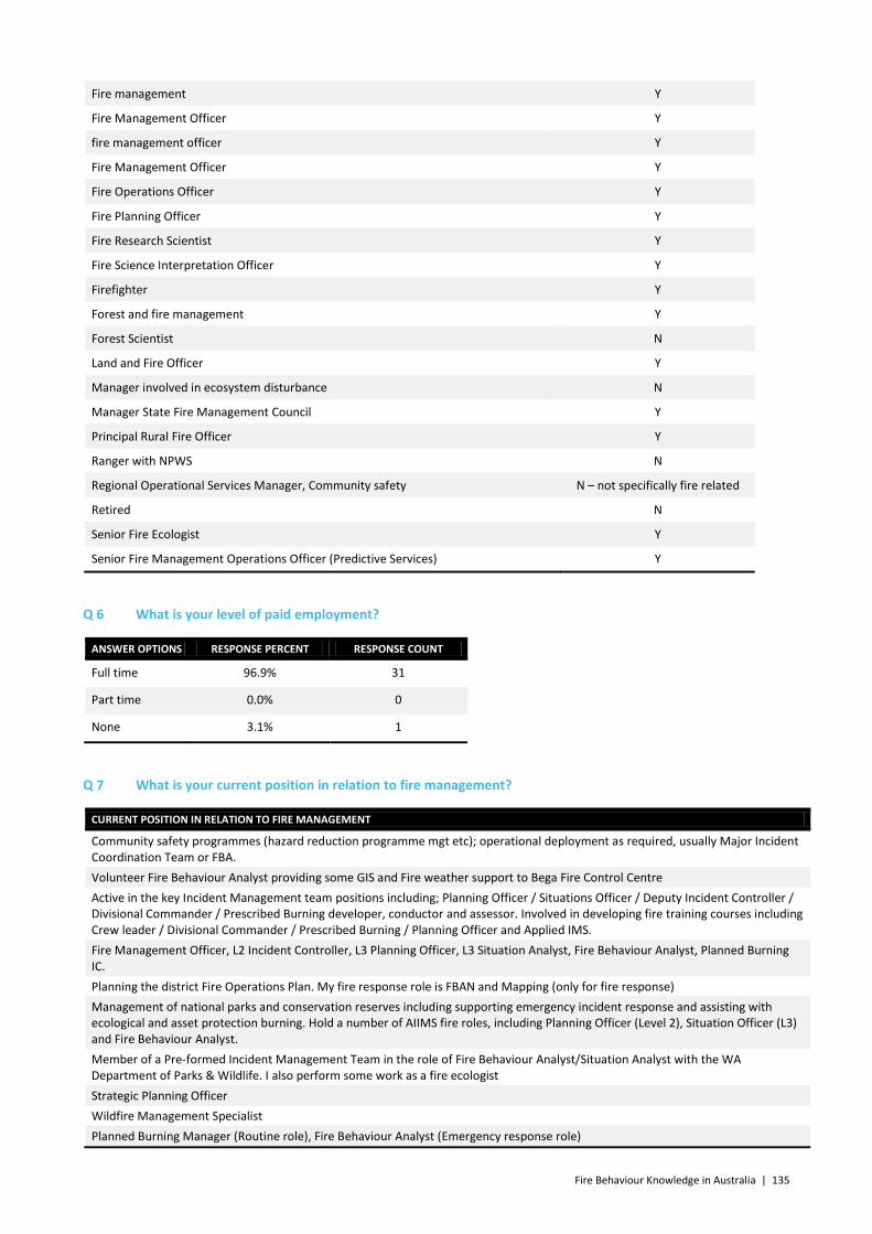
Fire Behaviour Knowledge in Australia | 135
Fire management Y
Fire Management Officer Y
fire management officer Y
Fire Management Officer Y
Fire Operations Officer Y
Fire Planning Officer Y
Fire Research Scientist Y
Fire Science Interpretation Officer Y
Firefighter Y
Forest and fire management Y
Forest Scientist N
Land and Fire Officer Y
Manager involved in ecosystem disturbance N
Manager State Fire Management Council Y
Principal Rural Fire Officer Y
Ranger with NPWS N
Regional Operational Services Manager, Community safety N – not specifically fire related
Retired N
Senior Fire Ecologist Y
Senior Fire Management Operations Officer (Predictive Services) Y
Q 6 What is your level of paid employment?
ANSWER OPTIONS RESPONSE PERCENT RESPONSE COUNT
Full time 96.9% 31
Part time 0.0% 0
None 3.1% 1
Q 7 What is your current position in relation to fire management?
CURRENT POSITION IN RELATION TO FIRE MANAGEMENT
Community safety programmes (hazard reduction programme mgt etc); operational deployment as required, usually Major Incident Coordination Team or FBA. Volunteer Fire Behaviour Analyst providing some GIS and Fire weather support to Bega Fire Control Centre Active in the key Incident Management team positions including; Planning Officer / Situations Officer / Deputy Incident Controller / Divisional Commander / Prescribed Burning developer, conductor and assessor. Involved in developing fire training courses including Crew leader / Divisional Commander / Prescribed Burning / Planning Officer and Applied IMS. Fire Management Officer, L2 Incident Controller, L3 Planning Officer, L3 Situation Analyst, Fire Behaviour Analyst, Planned Burning IC. Planning the district Fire Operations Plan. My fire response role is FBAN and Mapping (only for fire response) Management of national parks and conservation reserves including supporting emergency incident response and assisting with ecological and asset protection burning. Hold a number of AIIMS fire roles, including Planning Officer (Level 2), Situation Officer (L3) and Fire Behaviour Analyst. Member of a Pre-formed Incident Management Team in the role of Fire Behaviour Analyst/Situation Analyst with the WA Department of Parks & Wildlife. I also perform some work as a fire ecologist Strategic Planning Officer Wildfire Management Specialist Planned Burning Manager (Routine role), Fire Behaviour Analyst (Emergency response role)

136 | Fire Behaviour Knowledge in Australia
Fire behaviour analyst Senior Fire Ecologist Performance Management My current position is within the Department of Parks and Wildlife as a Conservation Officer which includes aspects of fire ecology and fire planning. During the fire season i perform roles where required as a Fire Behaviour analyst, Situation Unit Leader, Mapping and Sector Commander Season outlook, fire weather and fire behaviour information needs, fire behaviour analysis Fire Behaviour Specialist / Fire Behaviour Analyst Development of strategic fire plans, level 3 incident planning officer, environmental assessment of planned burns Principal Rural Fire Officer I manage a small unit that undertakes tenure blind bushfire risk management planning, and oversees local fire management area committees to cooperatively manage bushfire risk across all tenures. Manager Environmental Fire Research & Training Bushfire Risk Management Officer, Situation Officer, Operations Officer, Air Attack Supervisor Planning Officer on National Fire Management Team (1 of 3 teams). Just finished 5 years as deputy and then national fire coordinator in a government department Fire Behaviour Simulator Fire Behaviour Analyst, Situation Officer (Level 3), Operations Officer (Level 2), Burn Officer in Charge Fire Behaviour Analyst May undertake a number of Fire Management positions and supply Fire Behaviour relevant information to field crews. Senior Fire Operations Officer, State and regional Duty Office, Operations Officer on L3 Preformed team NPWS Fire & Incident Management Section. Fire Science Officer. Operational duties (mostly state level coordination) as required Preformed IMT Situation Analysis Fire Management Officer for NPWS NSW in the North Coast Region Senior Ranger - Fire
Q 8 What best describes your role?
ANSWER CHOICES RESPONSES
I work with a fire authority 11 34.38%
I work with a land management agency 19 59.38%
I have no formal association 0 0.00%
Other (please specify): 2 6.25%
Total 32
Q 9 Which of the following best describes the area where you work when undertaking fire behaviour analysis?
ANSWER CHOICES – RESPONSES –
State head office 16 50.00%
Regional office 4 12.50%
District office 5 15.63%
Other (please specify): 7 21.88%
Total 32
All of the above at various intervals over the last 3 years Both in a District Office and State Operations For emergency response in Incident Control Centre or State Control Centre), Planning at District Office National Incident Management Team (NIMT) or Regional Incident Management Team (RIMT) Regional Office, and MultiAgency Incident management Teams State, Regional and as Operations officer usually level 3 incidents
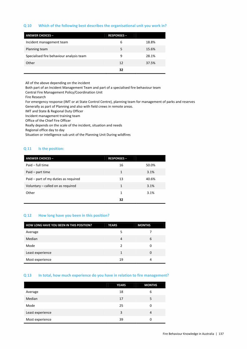
Fire Behaviour Knowledge in Australia | 137
Q 10 Which of the following best describes the organisational unit you work in?
ANSWER CHOICES – RESPONSES –
Incident management team 6 18.8%
Planning team 5 15.6%
Specialised fire behaviour analysis team 9 28.1%
Other 12 37.5%
32
All of the above depending on the incident Both part of an Incident Management Team and part of a specialised fire behaviour team Central Fire Management Policy/Coordination Unit Fire Research For emergency response (IMT or at State Control Centre), planning team for management of parks and reserves Generally as part of Planning and also with field crews in remote areas. IMT and State & Regional Duty Officer Incident management training team Office of the Chief Fire Officer Really depends on the scale of the incident, situation and needs Regional office day to day Situation or intelligence sub unit of the Planning Unit During wildfires
Q 11 Is the position:
ANSWER CHOICES – RESPONSES –
Paid – full time 16 50.0%
Paid – part time 1 3.1%
Paid – part of my duties as required 13 40.6%
Voluntary – called on as required 1 3.1%
Other 1 3.1%
32
Q 12 How long have you been in this position?
HOW LONG HAVE YOU BEEN IN THIS POSITION? YEARS MONTHS
Average 5 7
Median 4 6
Mode 2 0
Least experience 1 0
Most experience 19 4
Q 13 In total, how much experience do you have in relation to fire management?
YEARS MONTHS
Average 18 6
Median 17 5
Mode 25 0
Least experience 3 4
Most experience 39 0

138 | Fire Behaviour Knowledge in Australia
Q 14 My fire behaviour analysis covers an area which is:
24 FBANs were located at state HQ. The 8 that were located regionally were in very large regions
ANSWER CHOICES – RESPONSES –
State wide 75.0% 24
District/region specific 25.0% 8
32
Q 15 Have you been called upon to perform fire behaviour analysis in another state?
ANSWER CHOICES – RESPONSES –
Yes 28.1% 9
No 71.9% 23
32
B.2 Training
Q 16 What formal fire behaviour analyst training have you completed?
Advanced Fire Behaviour course 3
unspecified 1
Canada 2
Crew Leader Fire Behaviour NZ 1
Fire Behaviour Analysis course 22
unspecified 8
Australian national 1
DSE 1
Tolhurst 7
RFS 5
Fire Behaviour Refresher course 1
Fire Behaviour Specialist Canada 1
Fire Weather training 1
Intermediate Fire Behaviour 7
unspecified 2
Canada 1
DSE 3
NZ 1
Planning Officer course 1
Prometheus Fire Growth Modelling 1
Situation Unit Leader DPaW 1
Situation/Prediction course 1
Tech Transfer workshop 1
Wildland Fire Behaviour Specialist course
1
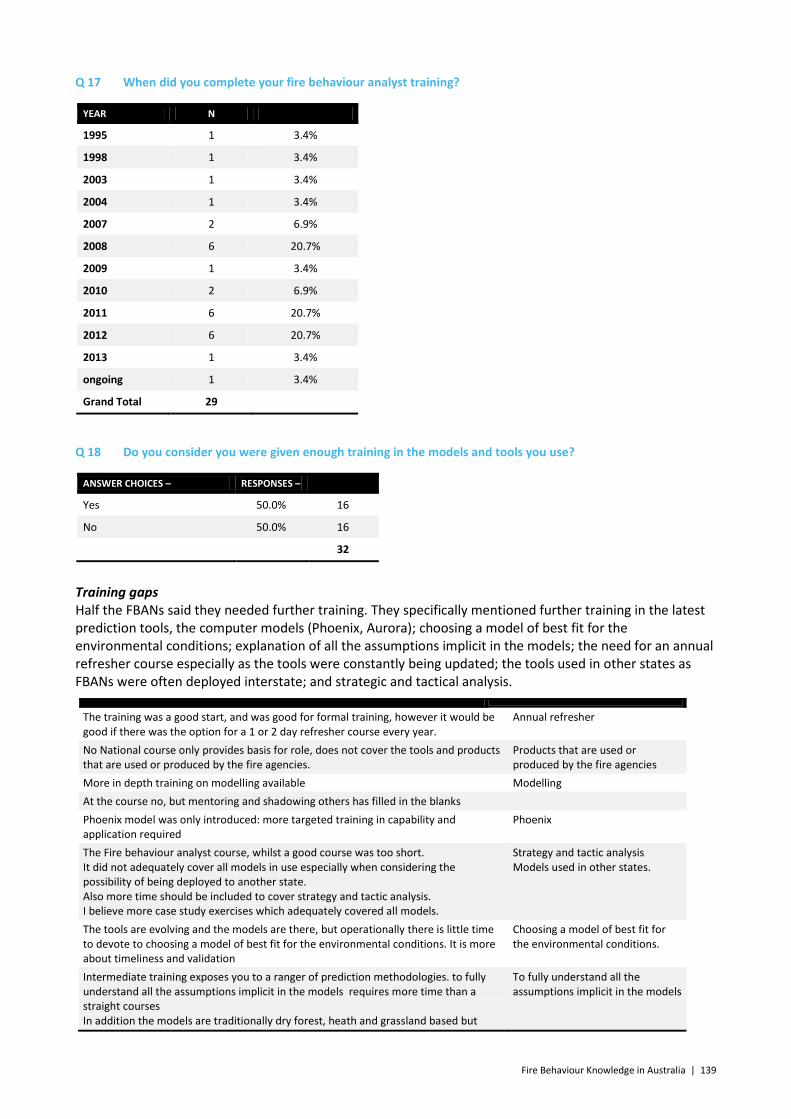
Fire Behaviour Knowledge in Australia | 139
Q 17 When did you complete your fire behaviour analyst training?
YEAR N
1995 1 3.4%
1998 1 3.4%
2003 1 3.4%
2004 1 3.4%
2007 2 6.9%
2008 6 20.7%
2009 1 3.4%
2010 2 6.9%
2011 6 20.7%
2012 6 20.7%
2013 1 3.4%
ongoing 1 3.4%
Grand Total 29
Q 18 Do you consider you were given enough training in the models and tools you use?
ANSWER CHOICES – RESPONSES –
Yes 50.0% 16
No 50.0% 16
32
Training gaps Half the FBANs said they needed further training. They specifically mentioned further training in the latest prediction tools, the computer models (Phoenix, Aurora); choosing a model of best fit for the environmental conditions; explanation of all the assumptions implicit in the models; the need for an annual refresher course especially as the tools were constantly being updated; the tools used in other states as FBANs were often deployed interstate; and strategic and tactical analysis.
The training was a good start, and was good for formal training, however it would be good if there was the option for a 1 or 2 day refresher course every year.
Annual refresher
No National course only provides basis for role, does not cover the tools and products that are used or produced by the fire agencies.
Products that are used or produced by the fire agencies
More in depth training on modelling available Modelling At the course no, but mentoring and shadowing others has filled in the blanks Phoenix model was only introduced: more targeted training in capability and application required
Phoenix
The Fire behaviour analyst course, whilst a good course was too short. It did not adequately cover all models in use especially when considering the possibility of being deployed to another state. Also more time should be included to cover strategy and tactic analysis. I believe more case study exercises which adequately covered all models.
Strategy and tactic analysis Models used in other states.
The tools are evolving and the models are there, but operationally there is little time to devote to choosing a model of best fit for the environmental conditions. It is more about timeliness and validation
Choosing a model of best fit for the environmental conditions.
Intermediate training exposes you to a ranger of prediction methodologies. to fully understand all the assumptions implicit in the models requires more time than a straight courses In addition the models are traditionally dry forest, heath and grassland based but
To fully understand all the assumptions implicit in the models

140 | Fire Behaviour Knowledge in Australia
there is an immense amount of different fuel types out there Not really been formally trained in Phoenix, though have been able to figure it out. No training with Aurora, limited training with Vesta.
Phoenix, Aurora, Vesta
No formal training in using fire behaviour computer models. Computer models The tools that are currently used have progressed considerably since I undertook training in 2008.
New tools
The training was sufficient initially but new tools were developed since the training and this had been taught on the job. It always takes a day to get used to new tools and procedures each year
New tools
At the time it was what was available, have looked at other models since with limited use of most, however can generally use information to produce a manual outcome.
New tools
Possibly enough training but without regular use there is definitely a need for a refresher
Refresher
See above
Q 19 There are a number of ways you can keep up-to-date with the latest developments in fire behaviour research. Have you:
YES – NO – TOTAL –
Read fire case studies 100.00% 32 0.00% 0 32
Participated in a fire case study 53.13% 17 46.88% 15 32
Attended refresher training 71.88% 23 28.13% 9 32
Attended more advanced training 25.00% 8 75.00% 24 32
Attended seminars/webinars/conferences 84.38% 27 15.63% 5 32
Read the latest research 90.63% 29 9.38% 3 32
Other Training Online forums, COMET courses on Meteorology, study tour, peer learning e.g. Prometheus, scenario analysis; discussions with researchers
As a group in Tasmania, we endeavour to get together annually to keep everyone up to date with models, lessons learnt etc. We have also taught each other to use Prometheus. Developed a session on fire predictions for the NPWS Planning Officer Course / also a session for the RFS Planning workshop discussions with researchers Study tour Each year there is a refresher. In a part time role cannot keep informed of all the new developments so full time fire roles can develop more specialised expertise. End of season debrief Sharing information through FBA Yahoo Group Sharing research output among FBAs via email FBA Discussion Group on Linkedin Haven’t attended formal refresher training but have worked with others to organise time each year to run through a scenario I am an active fire behaviour researcher I develop/design fire behaviour based decision support tools and systems I have had some discussions with peers as to gain better knowledge and use of online modelling tools. I manage the FBA function in SA I am chairing AFAC group to establish a National FBA capacity interaction between other fire specialists It forms a large part of my substantive role On job refresher and collegial learning Online FBA user group Online forums Undertaking COMET courses on Meteorology Improving and modifying Excel models to reduce workloads and reduce errors
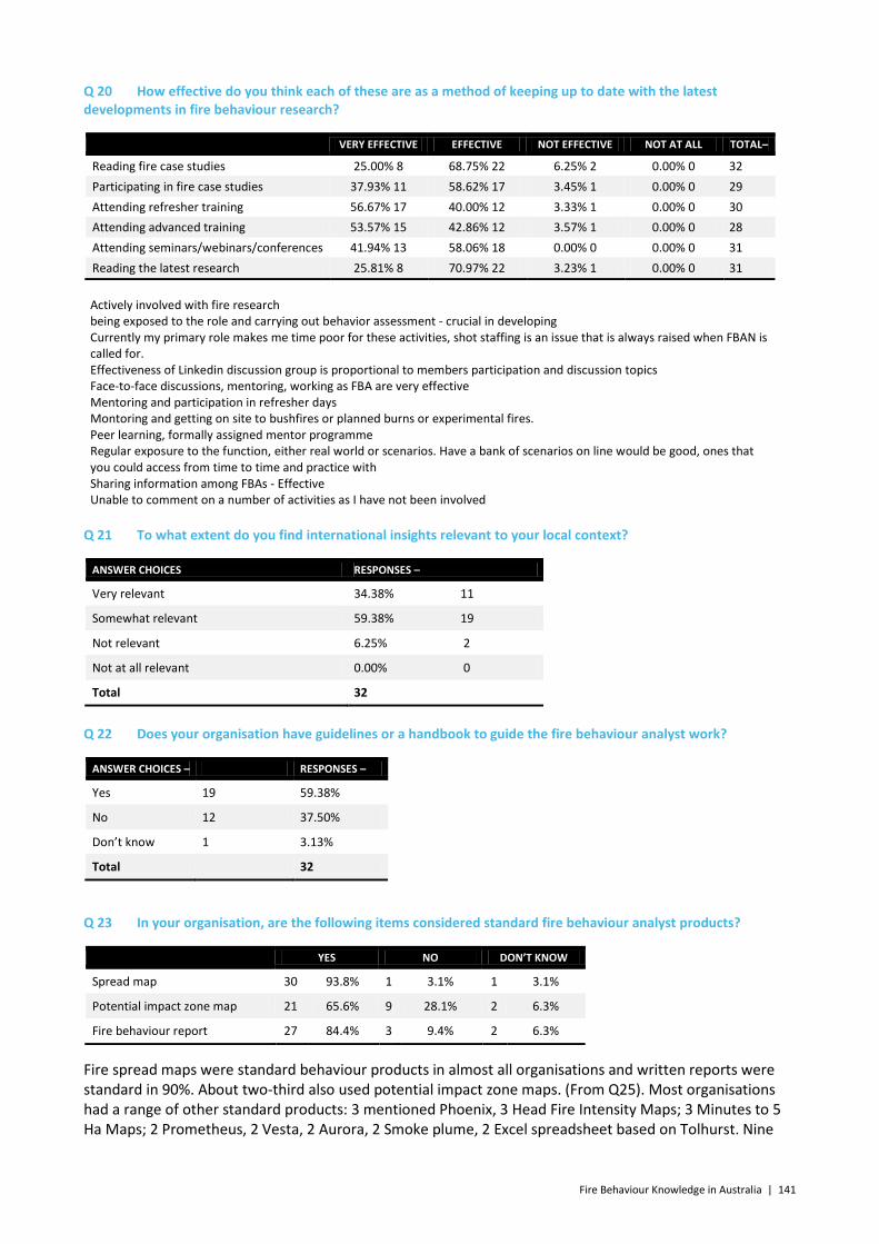
Fire Behaviour Knowledge in Australia | 141
Q 20 How effective do you think each of these are as a method of keeping up to date with the latest developments in fire behaviour research?
VERY EFFECTIVE EFFECTIVE NOT EFFECTIVE NOT AT ALL TOTAL–
Reading fire case studies 25.00% 8 68.75% 22 6.25% 2 0.00% 0 32 Participating in fire case studies 37.93% 11 58.62% 17 3.45% 1 0.00% 0 29 Attending refresher training 56.67% 17 40.00% 12 3.33% 1 0.00% 0 30 Attending advanced training 53.57% 15 42.86% 12 3.57% 1 0.00% 0 28 Attending seminars/webinars/conferences 41.94% 13 58.06% 18 0.00% 0 0.00% 0 31 Reading the latest research 25.81% 8 70.97% 22 3.23% 1 0.00% 0 31
Actively involved with fire research being exposed to the role and carrying out behavior assessment - crucial in developing Currently my primary role makes me time poor for these activities, shot staffing is an issue that is always raised when FBAN is called for. Effectiveness of Linkedin discussion group is proportional to members participation and discussion topics Face-to-face discussions, mentoring, working as FBA are very effective Mentoring and participation in refresher days Montoring and getting on site to bushfires or planned burns or experimental fires. Peer learning, formally assigned mentor programme Regular exposure to the function, either real world or scenarios. Have a bank of scenarios on line would be good, ones that you could access from time to time and practice with Sharing information among FBAs - Effective Unable to comment on a number of activities as I have not been involved
Q 21 To what extent do you find international insights relevant to your local context?
ANSWER CHOICES RESPONSES –
Very relevant 34.38% 11
Somewhat relevant 59.38% 19
Not relevant 6.25% 2
Not at all relevant 0.00% 0
Total 32
Q 22 Does your organisation have guidelines or a handbook to guide the fire behaviour analyst work?
ANSWER CHOICES – RESPONSES –
Yes 19 59.38%
No 12 37.50%
Don’t know 1 3.13%
Total 32
Q 23 In your organisation, are the following items considered standard fire behaviour analyst products?
YES NO DON’T KNOW
Spread map 30 93.8% 1 3.1% 1 3.1%
Potential impact zone map 21 65.6% 9 28.1% 2 6.3%
Fire behaviour report 27 84.4% 3 9.4% 2 6.3%
Fire spread maps were standard behaviour products in almost all organisations and written reports were standard in 90%. About two-third also used potential impact zone maps. (From Q25). Most organisations had a range of other standard products: 3 mentioned Phoenix, 3 Head Fire Intensity Maps; 3 Minutes to 5 Ha Maps; 2 Prometheus, 2 Vesta, 2 Aurora, 2 Smoke plume, 2 Excel spreadsheet based on Tolhurst. Nine
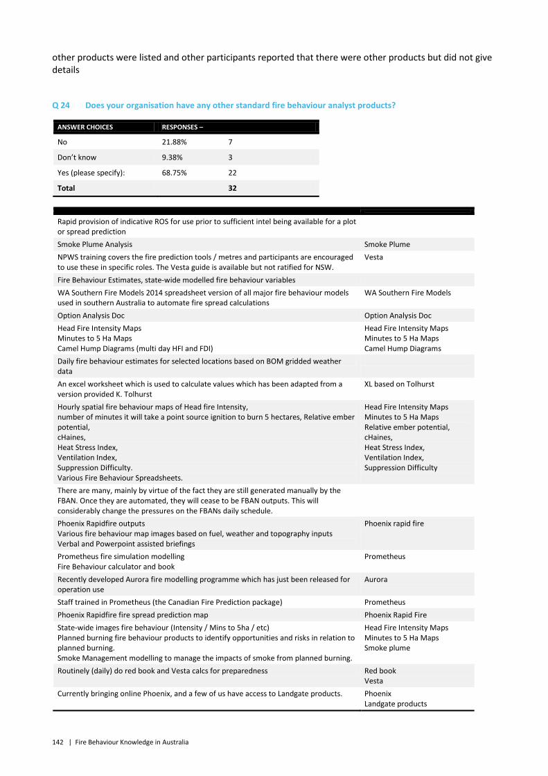
142 | Fire Behaviour Knowledge in Australia
other products were listed and other participants reported that there were other products but did not give details
Q 24 Does your organisation have any other standard fire behaviour analyst products?
ANSWER CHOICES RESPONSES –
No 21.88% 7
Don’t know 9.38% 3
Yes (please specify): 68.75% 22
Total 32
Rapid provision of indicative ROS for use prior to sufficient intel being available for a plot or spread prediction
Smoke Plume Analysis Smoke Plume NPWS training covers the fire prediction tools / metres and participants are encouraged to use these in specific roles. The Vesta guide is available but not ratified for NSW.
Vesta
Fire Behaviour Estimates, state-wide modelled fire behaviour variables WA Southern Fire Models 2014 spreadsheet version of all major fire behaviour models used in southern Australia to automate fire spread calculations
WA Southern Fire Models
Option Analysis Doc Option Analysis Doc Head Fire Intensity Maps Minutes to 5 Ha Maps Camel Hump Diagrams (multi day HFI and FDI)
Head Fire Intensity Maps Minutes to 5 Ha Maps Camel Hump Diagrams
Daily fire behaviour estimates for selected locations based on BOM gridded weather data
An excel worksheet which is used to calculate values which has been adapted from a version provided K. Tolhurst
XL based on Tolhurst
Hourly spatial fire behaviour maps of Head fire Intensity, number of minutes it will take a point source ignition to burn 5 hectares, Relative ember potential, cHaines, Heat Stress Index, Ventilation Index, Suppression Difficulty. Various Fire Behaviour Spreadsheets.
Head Fire Intensity Maps Minutes to 5 Ha Maps Relative ember potential, cHaines, Heat Stress Index, Ventilation Index, Suppression Difficulty
There are many, mainly by virtue of the fact they are still generated manually by the FBAN. Once they are automated, they will cease to be FBAN outputs. This will considerably change the pressures on the FBANs daily schedule.
Phoenix Rapidfire outputs Various fire behaviour map images based on fuel, weather and topography inputs Verbal and Powerpoint assisted briefings
Phoenix rapid fire
Prometheus fire simulation modelling Fire Behaviour calculator and book
Prometheus
Recently developed Aurora fire modelling programme which has just been released for operation use
Aurora
Staff trained in Prometheus (the Canadian Fire Prediction package) Prometheus Phoenix Rapidfire fire spread prediction map Phoenix Rapid Fire State-wide images fire behaviour (Intensity / Mins to 5ha / etc) Planned burning fire behaviour products to identify opportunities and risks in relation to planned burning. Smoke Management modelling to manage the impacts of smoke from planned burning.
Head Fire Intensity Maps Minutes to 5 Ha Maps Smoke plume
Routinely (daily) do red book and Vesta calcs for preparedness Red book Vesta
Currently bringing online Phoenix, and a few of us have access to Landgate products. Phoenix Landgate products
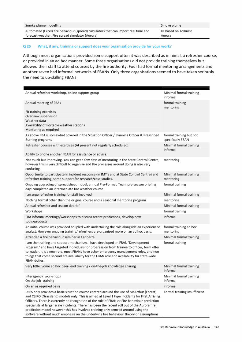
Fire Behaviour Knowledge in Australia | 143
Smoke plume modelling Smoke plume Automated (Excel) fire behaviour (spread) calculators that can import real time and forecast weather. Fire spread simulator (Aurora)
XL based on Tolhurst Aurora
Q 25 What, if any, training or support does your organisation provide for your work?
Although most organisations provided some support often it was described as minimal, a refresher course, or provided in an ad hoc manner. Some three organisations did not provide training themselves but allowed their staff to attend courses by the fire authority. Four had formal mentoring arrangements and another seven had informal networks of FBANs. Only three organisations seemed to have taken seriously the need to up-skilling FBANs
Annual refresher workshop, online support group Minimal formal training
informal Annual meeting of FBAs FB training exercises Overview supervision Weather data Availability of Portable weather stations Mentoring as required
formal training mentoring
As above FBA is somewhat covered in the Situation Officer / Planning Officer & Prescribed Burning programs
formal training but not specifically FBAN
Refresher courses with exercises (At present not regularly scheduled). Ability to phone another FBAN for assistance or advice.
Minimal formal training informal
Not much but improving. You can get a few days of mentoring in the State Control Centre, however this is very difficult to organise and the processes around doing is also very confusing.
mentoring
Opportunity to participate in incident response (in IMT's and at State Control Centre) and refresher training, some support for research/case studies.
Minimal formal training mentoring
Ongoing upgrading of spreadsheet model; annual Pre-Formed Team pre-season briefing day; completed an intermediate fire weather course
formal training
I arrange refresher training for staff involved Minimal formal training Nothing formal other than the original course and a seasonal mentoring program mentoring Annual refresher and season debrief Minimal formal training Workshops formal training FBA informal meetings/workshops to discuss recent predictions, develop new tools/products
informal
An initial course was provided coupled with undertaking the role alongside an experienced analyst. However ongoing training/refreshers are organised more on an ad hoc basis.
formal training ad hoc mentoring
Attended a fire behaviour seminar in Canberra Minimal formal training I am the training and support mechanism. I have developed an FBAN 'Development Program.' and have targeted individuals for progression from trainee to officer, form offer to leader. It is a new role, most FBANs have other emergency management roles, and two things that come second are availability for the FBAN role and availability for state-wide FBAN duties.
formal training
Very little. Some ad hoc peer-lead training / on-the-job knowledge sharing Minimal formal training informal
Interagency workshops On the job training
Minimal formal training informal
On an as required basis informal DFES only provides a basic situation course centred around the use of McArthur (Forest) and CSIRO (Grassland) models only. This is aimed at Level 1 type incidents for First Arriving Officers. There is currently no recognition of the role of FBAN or Fire behaviour prediction specialists at larger scale incidents. There has been the recent roll out of the Aurora fire prediction model however this has involved training only centred around using the software without much emphasis on the underlying fire behaviour theory or assumptions
Formal training insufficient
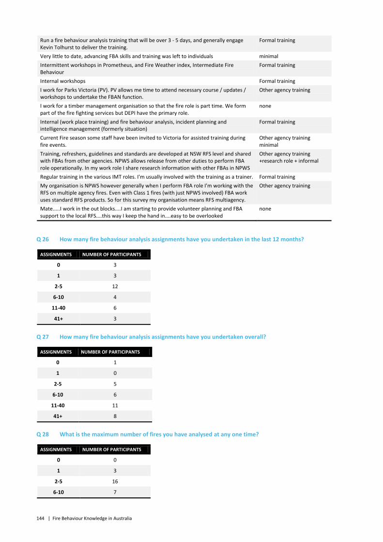
144 | Fire Behaviour Knowledge in Australia
Run a fire behaviour analysis training that will be over 3 - 5 days, and generally engage Kevin Tolhurst to deliver the training.
Formal training
Very little to date, advancing FBA skills and training was left to individuals minimal Intermittent workshops in Prometheus, and Fire Weather index, Intermediate Fire Behaviour
Formal training
Internal workshops Formal training I work for Parks Victoria (PV). PV allows me time to attend necessary course / updates / workshops to undertake the FBAN function.
Other agency training
I work for a timber management organisation so that the fire role is part time. We form part of the fire fighting services but DEPI have the primary role.
none
Internal (work place training) and fire behaviour analysis, incident planning and intelligence management (formerly situation)
Formal training
Current Fire season some staff have been invited to Victoria for assisted training during fire events.
Other agency training minimal
Training, refreshers, guidelines and standards are developed at NSW RFS level and shared with FBAs from other agencies. NPWS allows release from other duties to perform FBA role operationally. In my work role I share research information with other FBAs in NPWS
Other agency training +research role + informal
Regular training in the various IMT roles. I'm usually involved with the training as a trainer. Formal training My organisation is NPWS however generally when I perform FBA role I'm working with the RFS on multiple agency fires. Even with Class 1 fires (with just NPWS involved) FBA work uses standard RFS products. So for this survey my organisation means RFS multiagency.
Other agency training
Mate.....I work in the out blocks....I am starting to provide volunteer planning and FBA support to the local RFS....this way I keep the hand in....easy to be overlooked
none
Q 26 How many fire behaviour analysis assignments have you undertaken in the last 12 months?
ASSIGNMENTS NUMBER OF PARTICIPANTS
0 3
1 3
2-5 12
6-10 4
11-40 6
41+ 3
Q 27 How many fire behaviour analysis assignments have you undertaken overall?
ASSIGNMENTS NUMBER OF PARTICIPANTS
0 1
1 0
2-5 5
6-10 6
11-40 11
41+ 8
Q 28 What is the maximum number of fires you have analysed at any one time?
ASSIGNMENTS NUMBER OF PARTICIPANTS
0 0
1 3
2-5 16
6-10 7
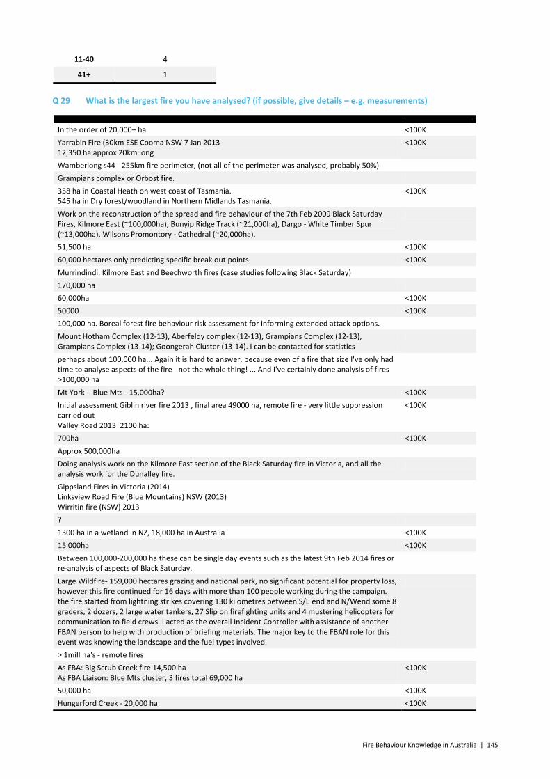
Fire Behaviour Knowledge in Australia | 145
11-40 4
41+ 1
Q 29 What is the largest fire you have analysed? (if possible, give details – e.g. measurements)
In the order of 20,000+ ha <100K Yarrabin Fire (30km ESE Cooma NSW 7 Jan 2013 12,350 ha approx 20km long
<100K
Wamberlong s44 - 255km fire perimeter, (not all of the perimeter was analysed, probably 50%) Grampians complex or Orbost fire. 358 ha in Coastal Heath on west coast of Tasmania. 545 ha in Dry forest/woodland in Northern Midlands Tasmania.
<100K
Work on the reconstruction of the spread and fire behaviour of the 7th Feb 2009 Black Saturday Fires, Kilmore East (~100,000ha), Bunyip Ridge Track (~21,000ha), Dargo - White Timber Spur (~13,000ha), Wilsons Promontory - Cathedral (~20,000ha).
51,500 ha <100K 60,000 hectares only predicting specific break out points <100K Murrindindi, Kilmore East and Beechworth fires (case studies following Black Saturday) 170,000 ha 60,000ha <100K 50000 <100K 100,000 ha. Boreal forest fire behaviour risk assessment for informing extended attack options. Mount Hotham Complex (12-13), Aberfeldy complex (12-13), Grampians Complex (12-13), Grampians Complex (13-14); Goongerah Cluster (13-14). I can be contacted for statistics
perhaps about 100,000 ha... Again it is hard to answer, because even of a fire that size I've only had time to analyse aspects of the fire - not the whole thing! ... And I've certainly done analysis of fires >100,000 ha
Mt York - Blue Mts - 15,000ha? <100K Initial assessment Giblin river fire 2013 , final area 49000 ha, remote fire - very little suppression carried out Valley Road 2013 2100 ha:
<100K
700ha <100K Approx 500,000ha Doing analysis work on the Kilmore East section of the Black Saturday fire in Victoria, and all the analysis work for the Dunalley fire.
Gippsland Fires in Victoria (2014) Linksview Road Fire (Blue Mountains) NSW (2013) Wirritin fire (NSW) 2013
? 1300 ha in a wetland in NZ, 18,000 ha in Australia <100K 15 000ha <100K Between 100,000-200,000 ha these can be single day events such as the latest 9th Feb 2014 fires or re-analysis of aspects of Black Saturday.
Large Wildfire- 159,000 hectares grazing and national park, no significant potential for property loss, however this fire continued for 16 days with more than 100 people working during the campaign. the fire started from lightning strikes covering 130 kilometres between S/E end and N/Wend some 8 graders, 2 dozers, 2 large water tankers, 27 Slip on firefighting units and 4 mustering helicopters for communication to field crews. I acted as the overall Incident Controller with assistance of another FBAN person to help with production of briefing materials. The major key to the FBAN role for this event was knowing the landscape and the fuel types involved.
> 1mill ha's - remote fires As FBA: Big Scrub Creek fire 14,500 ha As FBA Liaison: Blue Mts cluster, 3 fires total 69,000 ha
<100K
50,000 ha <100K Hungerford Creek - 20,000 ha <100K
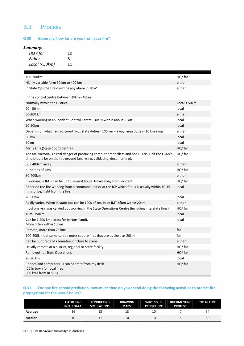
146 | Fire Behaviour Knowledge in Australia
B.3 Process
Q 30 Generally, how far are you from your fire?
Summary: HQ / far 10 Either 8 Local (<50km) 11
100-700km HQ/ far Highly variable form 30 km to 400 km either In State Ops the fire could be anywhere in NSW In the control centre between 15km - 40km
either
Normally within the District. Local < 50km 20 - 50 km local 50-200 km either When working in an Incident Control Centre usually within about 50km local 10-50km local Depends on what I am rostered for... state duties= 100 km + away, area duties= 10 km away either 50 km local 50km local Many kms (State Coord Centre) HQ/ far Too far. Victoria is a real danger of producing computer modellers and not FBANs. Half the FBAN's time should be on the fire ground (analysing, validating, documenting).
HQ/ far
50 - 400km away. either hundreds of kms HQ/ far 50-400km either If working in IMT- can be up to several hours travel away from incident HQ/ far Either on the fire working from a command unit or at the ICP which for us is usually within 10-15 mins drive/flight from the fire
local
20-50km local Really varies. When in state ops can be 100s of km, in an IMT often within 20km. either most analysis was carried out working in the State Operations Centre (including interstate fires) HQ/ far 10m- 150km local Can be 1,200 km (latest for in Northland). More often within 10 km
local
Remote, more than 25 kms far 100-200km but some can be outer suburb fires that are as close as 20km far Can be hundreds of kilometres or close to scene either Usually remote at a district, regional or State facility HQ/ far Removed - at State Operations HQ/ far 20-30 km local Phones and computers - I can operate from my desk. ICC in town for local fires 500 kms from RFS HO
HQ/ far
Q 31 For one fire spread prediction, how much time do you spend doing the following activities to predict fire propagation for the next 2 hours?
GATHERING INPUT DATA:
CONDUCTING SIMULATIONS:
DRAWING MAPS:
WRITING UP PREDICTION:
DOCUMENTING PROCESS:
TOTAL TIME
Average 16 13 13 10 7 54
Median 10 11 10 10 5 50
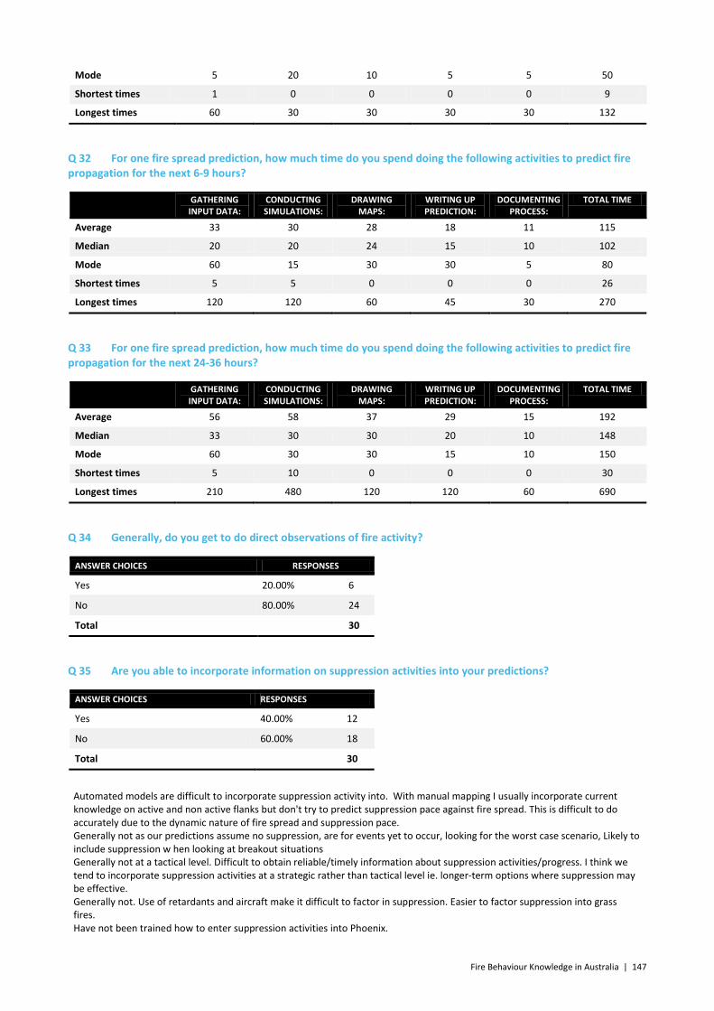
Fire Behaviour Knowledge in Australia | 147
Mode 5 20 10 5 5 50
Shortest times 1 0 0 0 0 9
Longest times 60 30 30 30 30 132
Q 32 For one fire spread prediction, how much time do you spend doing the following activities to predict fire propagation for the next 6-9 hours?
GATHERING INPUT DATA:
CONDUCTING SIMULATIONS:
DRAWING MAPS:
WRITING UP PREDICTION:
DOCUMENTING PROCESS:
TOTAL TIME
Average 33 30 28 18 11 115
Median 20 20 24 15 10 102
Mode 60 15 30 30 5 80
Shortest times 5 5 0 0 0 26
Longest times 120 120 60 45 30 270
Q 33 For one fire spread prediction, how much time do you spend doing the following activities to predict fire propagation for the next 24-36 hours?
GATHERING INPUT DATA:
CONDUCTING SIMULATIONS:
DRAWING MAPS:
WRITING UP PREDICTION:
DOCUMENTING PROCESS:
TOTAL TIME
Average 56 58 37 29 15 192
Median 33 30 30 20 10 148
Mode 60 30 30 15 10 150
Shortest times 5 10 0 0 0 30
Longest times 210 480 120 120 60 690
Q 34 Generally, do you get to do direct observations of fire activity?
ANSWER CHOICES RESPONSES
Yes 20.00% 6
No 80.00% 24
Total 30
Q 35 Are you able to incorporate information on suppression activities into your predictions?
ANSWER CHOICES RESPONSES
Yes 40.00% 12
No 60.00% 18
Total 30
Automated models are difficult to incorporate suppression activity into. With manual mapping I usually incorporate current knowledge on active and non active flanks but don't try to predict suppression pace against fire spread. This is difficult to do accurately due to the dynamic nature of fire spread and suppression pace. Generally not as our predictions assume no suppression, are for events yet to occur, looking for the worst case scenario, Likely to include suppression w hen looking at breakout situations Generally not at a tactical level. Difficult to obtain reliable/timely information about suppression activities/progress. I think we tend to incorporate suppression activities at a strategic rather than tactical level ie. longer-term options where suppression may be effective. Generally not. Use of retardants and aircraft make it difficult to factor in suppression. Easier to factor suppression into grass fires. Have not been trained how to enter suppression activities into Phoenix.

148 | Fire Behaviour Knowledge in Australia
I can, but, we are providing predictions without suppression input Manually into predictions Most analysis is carried out with no consideration of suppression activities or as a 'worst case' scenario. there should be scope to include fire predictions that consider backburning operations and suppression activities as this can drastically alter fire development most or prediction will be based on no suppression it is difficult to incorporate active suppression rates in a fire behaviour models Poorly modelled, and hard to verify from the field. Most of our predictions are used to identify worst case scenarios. Predictions generally run assuming no suppression. Use suppression info when providing multiple predictions or scenarios. Can be hard to get accurate, relevant, or immediate information on suppression from IMTs Simulation model has capability but it is not well developed Too many variables to accurately predict effect of suppression- some inbuilt assumptions about suppression are made by selecting points of ignition for simulations on a going fire Unable to get access to accurate field intelligence, no reliable suppression models, unable to access information about planned strategies and tactics Very little information available Very poor fire ground communication and feedback. We always assume no suppression, unless it is for an escape or re-ignition scenario from active edge We can but it's really a guess as to suppression success/effectiveness. When working from State Ops sometime difficult to get info from fireline or IMT if you dont have specific contacts
Q 36 How do you communicate fire spread projections/fire behaviour to the planning team/incident management team?
ANSWER CHOICES – RESPONSES –
Central fire database 40.00% 12
Telephone 63.33% 19
In person 80.00% 24
Email 56.67% 17
Total Respondents 30
Q 37 Which of the following do you use to communicate your predictions?
ANSWER CHOICES – RESPONSES –
Maps 100.00% 30
Graphs 20.00% 6
Other visuals 30.00% 9
Written report 80.00% 24
Verbal report 73.33% 22
Total Respondents 30
Q 38 How often do you get feedback from the planning team/incident management team?
ANSWER CHOICES – RESPONSES –
Regularly 40.00% 12
Occasionally 16.67% 5
Rarely 26.67% 8
Never 0.00% 0
Other (please specify): 16.67% 5
Total 30

Fire Behaviour Knowledge in Australia | 149
Q 39 Are your predictions used by any other group?
RESPONSES –
Public liaison 61.54% 16
Community warning preparation 92.31% 24
Restricted area response team 3.85% 1
Total Respondents: 26
Q 40 How often do you verify your predictions?
ANSWER CHOICES – RESPONSES –
Every hour 3.33% 1
Every 3 hours 0.00% 0
If requested 0.00% 0
If new information arrives 56.67% 17
Once per shift 0.00% 0
Once per day 0.00% 0
Other (please specify): 40.00% 12
Total 30
As new info arrives and daily as requested, or if new information arrives, depending on how busy we are it may not get done for a few days. By necessity, this varies in line with the timescale of the prediction Constant contact with field intel to adjust prediction Depends on the emerging situation and weather changes Depends on where I am. In NZ probably every 4 hours. In Aus once a 12 hour shift If requested AND If new information arrives if requested or when new information arrives, otherwise every 3 to 6 hours depending on fire situation If working in an IMT on a single incident, every 1 to 2 hours, if at region or state level 2 to 3 times per shift or as requested. it varies a lot. I try to seek new information if I ever have a lull It varies with business of the fire and IMT but try to get verification 3 - 4 hourly. Whenever time permits which is seldom. Poor fire ground feedback and there seems an operational reluctance to send FBANs to the fire ground
Q 41 Which best describes how you interact with the planning team/incident management team?
RESPONSES –
I seek input prior to making predictions 30.00% 9
I seek input after making predictions 0.00% 0
I seek input on an ongoing basis 53.33% 16
I don’t need to seek input as they provide me with directions 0.00% 0
I don’t seek input 0.00% 0
Other (please specify): 16.67% 5
Total 30
A combination of points 1 to 4, depending on situation I get both pull and push input. I provide output. It needs to be a consistent and fluid info exchange There is overall poor understanding by incident management teams as to how best to use FBANs. Tick the first two Usually I am the planning team

150 | Fire Behaviour Knowledge in Australia
Q 42 How often do you use the following sources of information to gauge the precision of your predictions?
ALMOST ALWAYS MOST OF THE TIME SOMETIMES NEVER TOTAL
Supervisor 23.33% 7 30.00% 9 40.00% 12 6.67% 2 30
Planning team 20.00% 6 40.00% 12 40.00% 12 0.00% 0 30
Incident management team 23.33% 7 26.67% 8 46.67% 14 3.33% 1 30
IR scan 26.67% 8 33.33% 10 23.33% 7 16.67% 5 30
Aerial observer 16.67% 5 33.33% 10 50.00% 15 0.00% 0 30
Social media 0.00% 0 0.00% 0 40.00% 12 60.00% 18 30
Agency software 26.67% 8 33.33% 10 20.00% 6 20.00% 6 30
Personal contact at the fire 23.33% 7 26.67% 8 46.67% 14 3.33% 1 30
SitReps 33.33% 10 30.00% 9 36.67% 11 0.00% 0 30
Q 43 How often do you have opportunity to check your predictions with observed fire behaviour?
ANSWER CHOICES RESPONSES
Almost always 6.67% 2
Most of the time 33.33% 10
Sometimes 56.67% 17
Never 3.33% 10
Total 30
Q 44 How do you go about making measurements of observed rates of fire spread?
Only 3 mentioned technical sources such as aerial mapping, IR line scans or databases but not ground observations. 5 mentioned on ground sources
• Ground observations by IMT or trained observers 17 • Personal observations 4 • SitReps 4 or Fireground 1 total 5 • Infra red Line Scans 7 • Comparing MODIS Hotspot data 1 • Aerial photos or mapping 9 • tracking data from on site equipment 1 • unclear whether ground or aerial photos - probably aerial 1 • just said GIS 1 • Just described calculation not source of data 2 • Does not happen / no time / no answer 4
I don't personally get to, however I always check my predictions with field intel via the IMT ground observers Line Scans Field reports ground observers
Line Scans Time the FROS for 10 minutes from an identified point, time the BROS for 10 minutes from an identified point.
calculation
Line of sight on the ground if possible. Reverse calculation of spread of fire between two known points and times.
Personal obs
Oblique aerial photos from aerial observer combined with GIS; aerial Air and Ground observers, IR scans, photographs ground observers
aerial
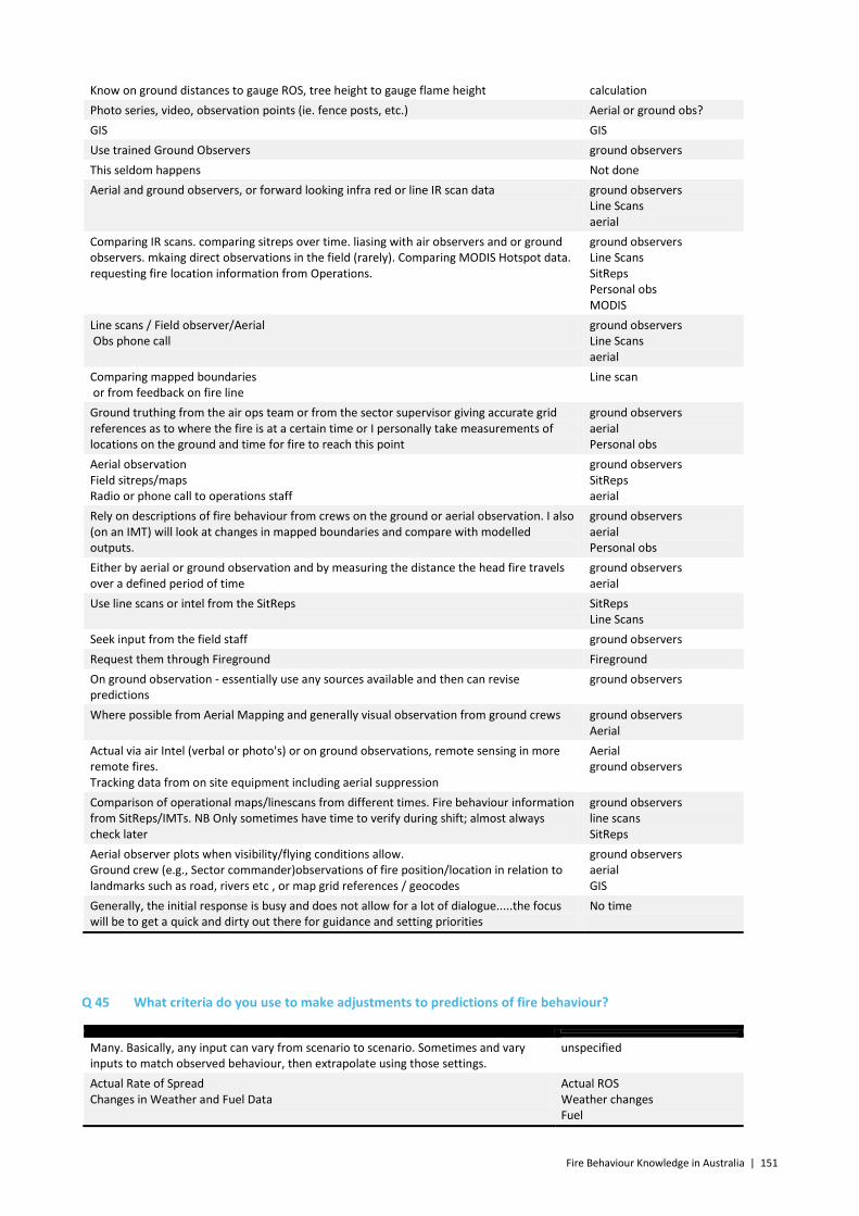
Fire Behaviour Knowledge in Australia | 151
Know on ground distances to gauge ROS, tree height to gauge flame height calculation Photo series, video, observation points (ie. fence posts, etc.) Aerial or ground obs? GIS GIS Use trained Ground Observers ground observers This seldom happens Not done Aerial and ground observers, or forward looking infra red or line IR scan data ground observers
Line Scans aerial
Comparing IR scans. comparing sitreps over time. liasing with air observers and or ground observers. mkaing direct observations in the field (rarely). Comparing MODIS Hotspot data. requesting fire location information from Operations.
ground observers Line Scans SitReps Personal obs MODIS
Line scans / Field observer/Aerial Obs phone call
ground observers Line Scans aerial
Comparing mapped boundaries or from feedback on fire line
Line scan
Ground truthing from the air ops team or from the sector supervisor giving accurate grid references as to where the fire is at a certain time or I personally take measurements of locations on the ground and time for fire to reach this point
ground observers aerial Personal obs
Aerial observation Field sitreps/maps Radio or phone call to operations staff
ground observers SitReps aerial
Rely on descriptions of fire behaviour from crews on the ground or aerial observation. I also (on an IMT) will look at changes in mapped boundaries and compare with modelled outputs.
ground observers aerial Personal obs
Either by aerial or ground observation and by measuring the distance the head fire travels over a defined period of time
ground observers aerial
Use line scans or intel from the SitReps SitReps Line Scans
Seek input from the field staff ground observers Request them through Fireground Fireground On ground observation - essentially use any sources available and then can revise predictions
ground observers
Where possible from Aerial Mapping and generally visual observation from ground crews ground observers Aerial
Actual via air Intel (verbal or photo's) or on ground observations, remote sensing in more remote fires. Tracking data from on site equipment including aerial suppression
Aerial ground observers
Comparison of operational maps/linescans from different times. Fire behaviour information from SitReps/IMTs. NB Only sometimes have time to verify during shift; almost always check later
ground observers line scans SitReps
Aerial observer plots when visibility/flying conditions allow. Ground crew (e.g., Sector commander)observations of fire position/location in relation to landmarks such as road, rivers etc , or map grid references / geocodes
ground observers aerial GIS
Generally, the initial response is busy and does not allow for a lot of dialogue.....the focus will be to get a quick and dirty out there for guidance and setting priorities
No time
Q 45 What criteria do you use to make adjustments to predictions of fire behaviour?
Many. Basically, any input can vary from scenario to scenario. Sometimes and vary inputs to match observed behaviour, then extrapolate using those settings.
unspecified
Actual Rate of Spread Changes in Weather and Fuel Data
Actual ROS Weather changes Fuel
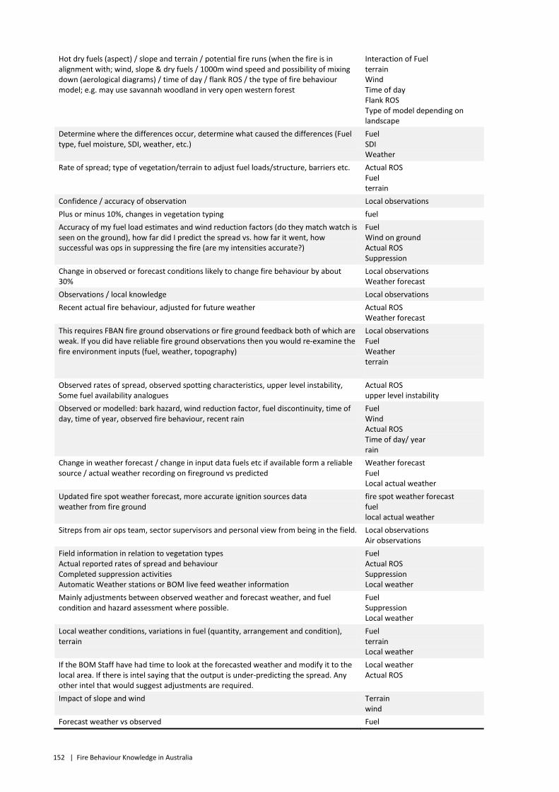
152 | Fire Behaviour Knowledge in Australia
Hot dry fuels (aspect) / slope and terrain / potential fire runs (when the fire is in alignment with; wind, slope & dry fuels / 1000m wind speed and possibility of mixing down (aerological diagrams) / time of day / flank ROS / the type of fire behaviour model; e.g. may use savannah woodland in very open western forest
Interaction of Fuel terrain Wind Time of day Flank ROS Type of model depending on landscape
Determine where the differences occur, determine what caused the differences (Fuel type, fuel moisture, SDI, weather, etc.)
Fuel SDI Weather
Rate of spread; type of vegetation/terrain to adjust fuel loads/structure, barriers etc. Actual ROS Fuel terrain
Confidence / accuracy of observation Local observations Plus or minus 10%, changes in vegetation typing fuel Accuracy of my fuel load estimates and wind reduction factors (do they match watch is seen on the ground), how far did I predict the spread vs. how far it went, how successful was ops in suppressing the fire (are my intensities accurate?)
Fuel Wind on ground Actual ROS Suppression
Change in observed or forecast conditions likely to change fire behaviour by about 30%
Local observations Weather forecast
Observations / local knowledge Local observations Recent actual fire behaviour, adjusted for future weather Actual ROS
Weather forecast This requires FBAN fire ground observations or fire ground feedback both of which are weak. If you did have reliable fire ground observations then you would re-examine the fire environment inputs (fuel, weather, topography)
Local observations Fuel Weather terrain
Observed rates of spread, observed spotting characteristics, upper level instability, Some fuel availability analogues
Actual ROS upper level instability
Observed or modelled: bark hazard, wind reduction factor, fuel discontinuity, time of day, time of year, observed fire behaviour, recent rain
Fuel Wind Actual ROS Time of day/ year rain
Change in weather forecast / change in input data fuels etc if available form a reliable source / actual weather recording on fireground vs predicted
Weather forecast Fuel Local actual weather
Updated fire spot weather forecast, more accurate ignition sources data weather from fire ground
fire spot weather forecast fuel local actual weather
Sitreps from air ops team, sector supervisors and personal view from being in the field. Local observations Air observations
Field information in relation to vegetation types Actual reported rates of spread and behaviour Completed suppression activities Automatic Weather stations or BOM live feed weather information
Fuel Actual ROS Suppression Local weather
Mainly adjustments between observed weather and forecast weather, and fuel condition and hazard assessment where possible.
Fuel Suppression Local weather
Local weather conditions, variations in fuel (quantity, arrangement and condition), terrain
Fuel terrain Local weather
If the BOM Staff have had time to look at the forecasted weather and modify it to the local area. If there is intel saying that the output is under-predicting the spread. Any other intel that would suggest adjustments are required.
Local weather Actual ROS
Impact of slope and wind Terrain wind
Forecast weather vs observed Fuel

Fire Behaviour Knowledge in Australia | 153
Modelled fuel loads vs actual Modelled fuel moisture vs actual
Local weather
On ground observations or IR, air obs - whatever is available Local observations Air observations
Weather, Fuel levels and types, topography and previous fire scars. Fuel terrain weather previous fires
Depends on discrepancy: Compare observed to forecast weather and adjust. Account for suppression success. Verify fuel/vegetation data inputs with other sources. Use a different model and compare calculated RoS. Account for more or less spotting.
Fuel Actual ROS Suppression Local weather Different model/ Spotting amount
Actual recent historical/known fire spread - I use this to 'calibrate' my predictions. Sometimes, I obtain actual field weather and fuel inputs rather than forecast or predicted.
previous fire spread Fuel Local weather
Local knowledge Grassland condition
Local observations fuel
Q 46 How often do you revise your predictions?
ANSWER CHOICES – RESPONSES –
– Every hour 0.00% 0
– Every 3 hours 0.00% 0
– If requested 0.00% 0
– If new information arrives 63.33% 19
– Once per shift 0.00% 0
– Once per day 0.00% 0
– Other (please specify): 36.67% 11
Total 30
As new information arrives on fire spread, suppression activities and weather. As required but without feedback the only assumption that can be made is the prediction was accurate. as required or if new information arrives AND time permits daily and as new relevant info becomes available eg revised forecast or satellite pass depends on the amount of resources in planning team n as to weather in can get the opportunity to revises the prediction within an operational period depends on the number of fires and workload, perhaps twice a day or when new information or variation from the current prediction is noticed if requested or if new information arrives, otherwise every 3-6 hours depending on situation If requested OR If new information OR If have time Only if input data is wrong or inaccurate really dependant where I am working, and for how long. In state ops it is very reactive, on an IMT it is more structured. Varies from situation to situation - this can't be generalised
Q 47 How adequate is the process you use for predicting fire behaviour?
ANSWER CHOICES RESPONSES
Very good 3 10.0%
Good 13 43.3%
Fair 13 43.3%
Poor 1 3.3%
Total 30
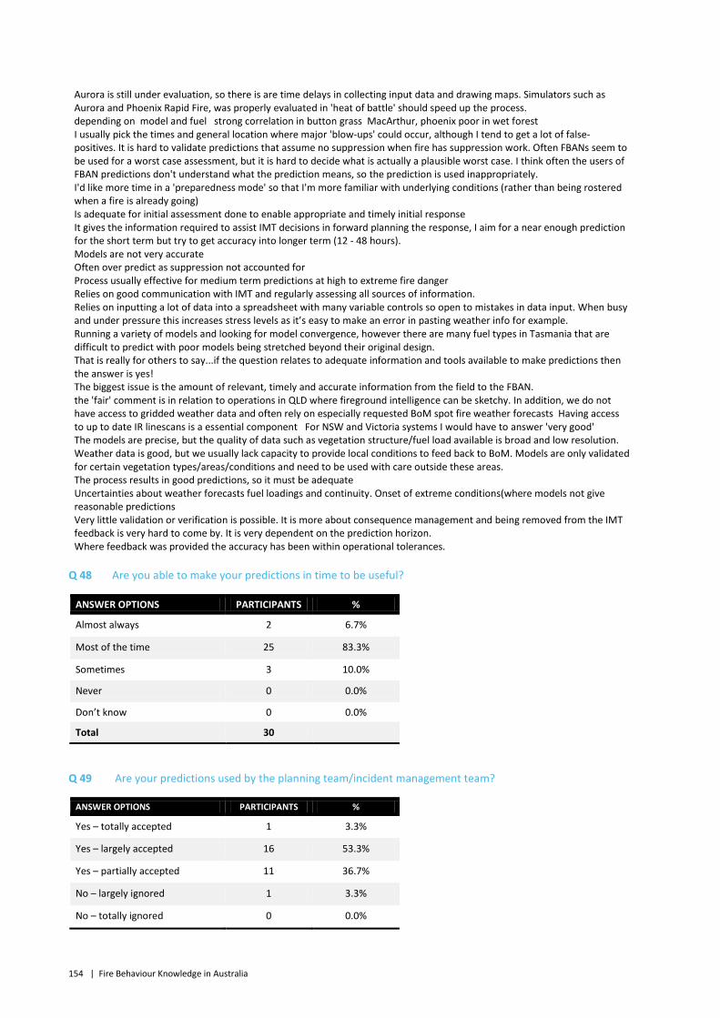
154 | Fire Behaviour Knowledge in Australia
Aurora is still under evaluation, so there is are time delays in collecting input data and drawing maps. Simulators such as Aurora and Phoenix Rapid Fire, was properly evaluated in 'heat of battle' should speed up the process. depending on model and fuel strong correlation in button grass MacArthur, phoenix poor in wet forest I usually pick the times and general location where major 'blow-ups' could occur, although I tend to get a lot of false-positives. It is hard to validate predictions that assume no suppression when fire has suppression work. Often FBANs seem to be used for a worst case assessment, but it is hard to decide what is actually a plausible worst case. I think often the users of FBAN predictions don't understand what the prediction means, so the prediction is used inappropriately. I'd like more time in a 'preparedness mode' so that I'm more familiar with underlying conditions (rather than being rostered when a fire is already going) Is adequate for initial assessment done to enable appropriate and timely initial response It gives the information required to assist IMT decisions in forward planning the response, I aim for a near enough prediction for the short term but try to get accuracy into longer term (12 - 48 hours). Models are not very accurate Often over predict as suppression not accounted for Process usually effective for medium term predictions at high to extreme fire danger Relies on good communication with IMT and regularly assessing all sources of information. Relies on inputting a lot of data into a spreadsheet with many variable controls so open to mistakes in data input. When busy and under pressure this increases stress levels as it’s easy to make an error in pasting weather info for example. Running a variety of models and looking for model convergence, however there are many fuel types in Tasmania that are difficult to predict with poor models being stretched beyond their original design. That is really for others to say...if the question relates to adequate information and tools available to make predictions then the answer is yes! The biggest issue is the amount of relevant, timely and accurate information from the field to the FBAN. the 'fair' comment is in relation to operations in QLD where fireground intelligence can be sketchy. In addition, we do not have access to gridded weather data and often rely on especially requested BoM spot fire weather forecasts Having access to up to date IR linescans is a essential component For NSW and Victoria systems I would have to answer 'very good' The models are precise, but the quality of data such as vegetation structure/fuel load available is broad and low resolution. Weather data is good, but we usually lack capacity to provide local conditions to feed back to BoM. Models are only validated for certain vegetation types/areas/conditions and need to be used with care outside these areas. The process results in good predictions, so it must be adequate Uncertainties about weather forecasts fuel loadings and continuity. Onset of extreme conditions(where models not give reasonable predictions Very little validation or verification is possible. It is more about consequence management and being removed from the IMT feedback is very hard to come by. It is very dependent on the prediction horizon. Where feedback was provided the accuracy has been within operational tolerances.
Q 48 Are you able to make your predictions in time to be useful?
ANSWER OPTIONS PARTICIPANTS %
Almost always 2 6.7%
Most of the time 25 83.3%
Sometimes 3 10.0%
Never 0 0.0%
Don’t know 0 0.0%
Total 30
Q 49 Are your predictions used by the planning team/incident management team?
ANSWER OPTIONS PARTICIPANTS %
Yes – totally accepted 1 3.3%
Yes – largely accepted 16 53.3%
Yes – partially accepted 11 36.7%
No – largely ignored 1 3.3%
No – totally ignored 0 0.0%

Fire Behaviour Knowledge in Australia | 155
Don't know 1 3.3%
Total 30
B.4 Fire prediction tools and simulation models
Q 50 My knowledge of the fire behaviour models that I commonly use is:
ANSWER OPTIONS PARTICIPANTS %
Excellent 5 16.7%
Good 22 73.3%
Fair 3 10.0%
Poor 0 0.0%
answered question 30
Q 51 How confident are you in the models you commonly use to predict fire behaviour?
ANSWER OPTIONS PARTICIPANTS %
Very confident 1 3.3%
Confident 27 90.0%
Not confident 2 6.7%
Not at all confident 0 0.0%
answered question 30
Q 52 For a given fire propagation scenario do you use a single model or combine outputs from distinct models?
ANSWER OPTIONS PARTICIPANTS %
Single model 7 23.3%
Combine outputs 23 76.7%
answered question 30
Q 53 How often do you use the following fire spread models for GRASSLAND areas?
MOST THE TIME ALMOST ALWAYS SOMETIMES OUT DATED NOT TRAINED OTHER REASON N
McArthur Mk 3 (McArthur 1973) 1 3.6% 0 0.0% 4 14.3% 14 50.0% 1 3.6% 8 28.6% 28
McArthur Mk 5 (McArthur 1977) 5 17.2% 4 13.8% 6 20.7% 4 13.8% 0 0.0% 10 34.5% 29
Purton GFDI (Purton 1982) 2 6.9% 1 3.4% 2 6.9% 3 10.3% 11 37.9% 10 34.5% 29
CSIRO grassland meter (Cheney et al. 1998)
9 32.1% 12 42.9% 5 17.9% 0 0.0% 0 0.0% 2 7.1% 28
Northern grassland equation (Cheney et al. 1998)
4 14.3% 1 3.6% 5 17.9% 0 0.0% 6 21.4% 12 42.9% 28
Central Australia spinifex (Griffin and Allan 1984)
0 0.0% 0 0.0% 1 3.4% 1 3.4% 11 37.9% 16 55.2% 29
Gibson desert 0 0.0% 1 3.4% 2 6.9% 0 0.0% 10 34.5% 16 55.2% 29
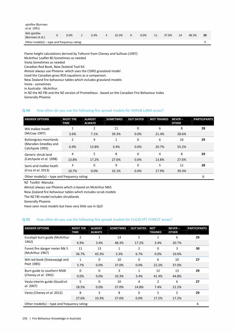
156 | Fire Behaviour Knowledge in Australia
spinifex (Burrows et al. 1991) WA spinifex (Burrows et al.) 0 0.0% 1 3.4% 3 10.3% 0 0.0% 11 37.9% 14 48.3% 29
Other model(s) – type and frequency rating: 9
Flame height calculations derived by Tolhurst from Cheney and Sullivan (1997) McArthur Leaflet 80 Sometimes as needed Vesta Sometimes as needed Canadian Red Book, New Zealand Tool Kit Almost always use Phoenix- which uses the CSIRO grassland model Used the Canadian grass ROS equations as a comparison. New Zealand fire behaviour tables which includes grassland models Vesta - sometimes In Australia - McArthur. In NZ the NZ FBI and the NZ version of Prometheus - based on the Canadian Fire Behaviour Index Generally Phoenix
Q 54 How often do you use the following fire spread models for SHRUB LAND areas?
ANSWER OPTIONS MOST THE TIME
ALMOST ALWAYS
SOMETIMES OUT DATED NOT TRAINED NEVER – OTHER
PARTICIPANTS
WA mallee-heath (McCaw 1997)
1 2 11 0 6 8 28
3.6% 7.1% 39.3% 0.0% 21.4% 28.6% Buttongrass moorlands (Marsden-Smedley and Catchpole 1995)
2 4 1 0 6 16 29
6.9% 13.8% 3.4% 0.0% 20.7% 55.2%
Generic shrub land (Catchpole et al. 1998)
4 5 8 0 4 8 29
13.8% 17.2% 27.6% 0.0% 13.8% 27.6% Semi-arid mallee heath (Cruz et al. 2013)
3 0 9 0 5 11 28
10.7% 0.0% 32.1% 0.0% 17.9% 39.3% Other model(s) – type and frequency rating: 6
NZ Toolkit -Manuka Almost always use Phoenix which is based on McArthur Mk5 New Zealand fire behaviour tables which includes scrub models The NZ FBI model includes shrublands Generally Phoenix Have seen most models but have very little use in QLD
Q 55 How often do you use the following fire spread models for EUCALYPT FOREST areas?
ANSWER OPTIONS MOST THE TIME
ALMOST ALWAYS
SOMETIMES OUT DATED NOT TRAINED
NEVER – OTHER
PARTICIPANTS
Eucalypt burn guide (McArthur 1962)
2 1 14 5 1 6 29 6.9% 3.4% 48.3% 17.2% 3.4% 20.7%
Forest fire danger meter Mk 5 (McArthur 1967)
11 13 1 2 0 3 30 36.7% 43.3% 3.3% 6.7% 0.0% 10.0%
WA red book (Sneeuwjagt and Peet 1985)
1 0 10 0 6 10 27 3.7% 0.0% 37.0% 0.0% 22.2% 37.0%
Burn guide to southern NSW (Cheney et al. 1992)
0 0 3 1 12 13 29 0.0% 0.0% 10.3% 3.4% 41.4% 44.8%
Vesta interim guide (Gould et al. 2007)
5 0 10 4 2 6 27 18.5% 0.0% 37.0% 14.8% 7.4% 22.2%
Vesta (Cheney et al. 2012) 8 3 8 0 5 5 29 27.6% 10.3% 27.6% 0.0% 17.2% 17.2%
Other model(s) – type and frequency rating: 6
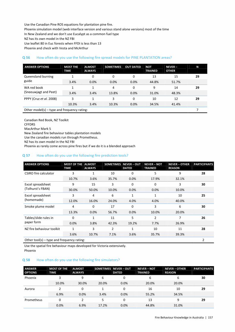
Fire Behaviour Knowledge in Australia | 157
Use the Canadian Pine ROS equations for plantation pine fire. Phoenix simulation model (web interface version and various stand alone versions) most of the time In New Zealand and we don't use Eucalypt as a common fuel type NZ has its own model in the NZ FBI Use leaflet 80 in Euc forests when FFDI is less than 13 Phoenix and check with Vesta and McArthur
Q 56 How often do you use the following fire spread models for PINE PLANTATION areas?
ANSWER OPTIONS MOST THE TIME
ALMOST ALWAYS
SOMETIMES OUT DATED NOT TRAINED
NEVER – OTHER
N
Queensland burning guide
1 0 0 0 13 15 29 3.4% 0.0% 0.0% 0.0% 44.8% 51.7%
WA red book (Sneeuwjagt and Peet)
1 1 4 0 9 14 29 3.4% 3.4% 13.8% 0.0% 31.0% 48.3%
PPPY (Cruz et al. 2008) 3 1 3 0 10 12 29 10.3% 3.4% 10.3% 0.0% 34.5% 41.4%
Other model(s) – type and frequency rating: 7
Canadian Red Book, NZ Toolkit CFFDRS MacArthur Mark 5 New Zealand fire behaviour tables plantation models Use the canadian models run through Prometheus. NZ has its own model in the NZ FBI Phoenix as rarely come across pine fires but if we do it is a blended approach
Q 57 How often do you use the following fire prediction tools?
ANSWER OPTIONS MOST OF THE TIME
ALMOST ALWAYS
SOMETIMES NEVER – OUT DATED
NEVER – NOT TRAINED
NEVER – OTHER REASON
PARTICIPANTS
CSIRO fire calculator 3 1 10 0 5 9 28 10.7% 3.6% 35.7% 0.0% 17.9% 32.1%
Excel spreadsheet (Tolhurst’s FBAN)
9 15 3 0 0 3 30 30.0% 50.0% 10.0% 0.0% 0.0% 10.0%
Excel spreadsheet (homemade)
3 4 6 1 1 10 25 12.0% 16.0% 24.0% 4.0% 4.0% 40.0%
Smoke plume model 4 0 17 0 3 6 30
13.3% 0.0% 56.7% 0.0% 10.0% 20.0%
Tables/slide rules in paper form
0 1 11 5 2 7 26 0.0% 3.8% 42.3% 19.2% 7.7% 26.9%
NZ fire behaviour toolkit 1 3 2 1 10 11 28 3.6% 10.7% 7.1% 3.6% 35.7% 39.3%
Other tool(s) – type and frequency rating: 2
Use the spatial fire behaviour maps developed for Victoria extensively. Phoenix
Q 58 How often do you use the following fire simulators?
ANSWER OPTIONS
MOST OF THE TIME
ALMOST ALWAYS
SOMETIMES NEVER – OUT DATED
NEVER – NOT TRAINED
NEVER – OTHER REASON
PARTICIPANTS
Phoenix 3 9 6 0 6 6 30 10.0% 30.0% 20.0% 0.0% 20.0% 20.0%
Aurora 2 0 1 0 16 10 29 6.9% 0.0% 3.4% 0.0% 55.2% 34.5%
Prometheus 0 2 5 0 13 9 29 0.0% 6.9% 17.2% 0.0% 44.8% 31.0%
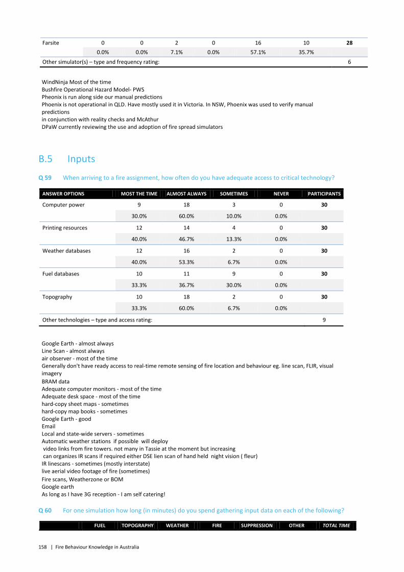
158 | Fire Behaviour Knowledge in Australia
Farsite 0 0 2 0 16 10 28 0.0% 0.0% 7.1% 0.0% 57.1% 35.7%
Other simulator(s) – type and frequency rating: 6
WindNinja Most of the time Bushfire Operational Hazard Model- PWS Pheonix is run along side our manual predictions Phoenix is not operational in QLD. Have mostly used it in Victoria. In NSW, Phoenix was used to verify manual predictions in conjunction with reality checks and McAthur DPaW currently reviewing the use and adoption of fire spread simulators
B.5 Inputs
Q 59 When arriving to a fire assignment, how often do you have adequate access to critical technology?
ANSWER OPTIONS MOST THE TIME ALMOST ALWAYS SOMETIMES NEVER PARTICIPANTS
Computer power 9 18 3 0 30
30.0% 60.0% 10.0% 0.0%
Printing resources 12 14 4 0 30
40.0% 46.7% 13.3% 0.0%
Weather databases 12 16 2 0 30
40.0% 53.3% 6.7% 0.0%
Fuel databases 10 11 9 0 30
33.3% 36.7% 30.0% 0.0%
Topography 10 18 2 0 30
33.3% 60.0% 6.7% 0.0%
Other technologies – type and access rating: 9
Google Earth - almost always Line Scan - almost always air observer - most of the time Generally don't have ready access to real-time remote sensing of fire location and behaviour eg. line scan, FLIR, visual imagery BRAM data Adequate computer monitors - most of the time Adequate desk space - most of the time hard-copy sheet maps - sometimes hard-copy map books - sometimes Google Earth - good Email Local and state-wide servers - sometimes Automatic weather stations if possible will deploy video links from fire towers. not many in Tassie at the moment but increasing can organizes IR scans if required either DSE lien scan of hand held night vision ( fleur) IR linescans - sometimes (mostly interstate) live aerial video footage of fire (sometimes) Fire scans, Weatherzone or BOM Google earth As long as I have 3G reception - I am self catering!
Q 60 For one simulation how long (in minutes) do you spend gathering input data on each of the following?
FUEL TOPOGRAPHY WEATHER FIRE SUPPRESSION OTHER TOTAL TIME

Fire Behaviour Knowledge in Australia | 159
LOCATION INFORMATION INPUT(S)
Average 12 7 17 15 12 14 61 Median 10 5 10 10 5 10 50 Mode 10 5 10 5 5 10 10 Shortest time 0 0 0 1 0 0 7 Longest time 60 30 45 90 90 60 280
Q 61 How often do you have the following to help with gathering data or interpretation?
ANSWER OPTIONS MOST THE TIME ALMOST ALWAYS SOMETIMES NEVER PARTICIPANTS
GIS officer
9 2 17 2 30 30.0% 6.7% 56.7% 6.7%
BOM forecaster
12 10 8 0 30 40.0% 33.3% 26.7% 0.0%
Local reconnaissance team
6 1 18 5 30 20.0% 3.3% 60.0% 16.7%
Supervisor
10 2 13 5 30 33.3% 6.7% 43.3% 16.7%
Colleague within agency
13 2 15 0 30 43.3% 6.7% 50.0% 0.0%
Other colleague
5 1 19 5 30 16.7% 3.3% 63.3% 16.7%
Other – type and frequency rating: 8
Ground / Air Observers Have State GIS Data available on portable drives almost always Existing map files on veg, topo, fire history, etc, almost always. State Predictive Services (Most of the time) local knowledge, i.e. forestry officer or brigade captain if available pick their brains as to fuel status IMT or Planning Section - sometimes Only in 2007 in Victoria really depends on prediction. Use any resource available ot improve predictions
B.5.1 INPUTS - WEATHER Q 62 Where do you get your weather forecast data?
ANSWER OPTIONS MOST OF THE TIME ALMOST ALWAYS SOMETIMES NEVER PARTICIPANTS
BOM public web site 7 4 17 1 29 24.1% 13.8% 58.6% 3.4%
BOM spot fire weather forecast
9 12 8 1 30 30.0% 40.0% 26.7% 3.3%
Download gridded weather
6 16 6 1 29 20.7% 55.2% 20.7% 3.4%
BOM registered user pages
6 16 5 3 30 20.0% 53.3% 16.7% 10.0%
Met Eye 9 7 11 3 30 30.0% 23.3% 36.7% 10.0%
Other forecast site (e.g. Elders, Weatherzone)
6 5 12 4 27
22.2% 18.5% 44.4% 14.8%
Other source(s) – type and frequency rating: 11
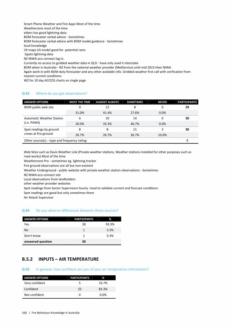
160 | Fire Behaviour Knowledge in Australia
Smart Phone Weather and Fire Apps Most of the time Weatherzone most of the time elders has good lightning data BOM forecaster verbal advice - Sometimes BOM forecaster verbal advice with BOM model guidance - Sometimes local knowledge VX maps US model good for potential rains Gpats lightning data NZ NIWA eco connect log in. Currently no access to gridded weather data in QLD - have only used it interstate BOM when in Australia - NZ from the national weather provider (MetService) until mid 2013 then NIWA Again work in with BOM duty forecaster and any other available info. Gridded weather first call with verification from nearest current conditions WZ for 10 day ACCESS charts on single page
Q 63 Where do you get observations?
ANSWER OPTIONS MOST THE TIME ALMOST ALWAYS SOMETIMES NEVER PARTICIPANTS
BOM public web site 9 12 8 0 29
31.0% 41.4% 27.6% 0.0%
Automatic Weather Station (i.e. PAWS)
6 10 14 0 30
20.0% 33.3% 46.7% 0.0%
Spot readings by ground crews at fire ground
8 8 11 3 30
26.7% 26.7% 36.7% 10.0%
Other source(s) – type and frequency rating: 9
Web Sites such as Davis Weather Link (Private weather stations, Weather stations installed for other purposes such as road works) Most of the time Weatherzone Pro - sometimes eg. lightning tracker Fire ground observations are all but non-existent Weather Underground - public website with private weather station observations - Sometimes NZ NIWA eco connect site Local observations from landholders other weather provider websites Spot readings from Sector Supervisors hourly. Used to validate current and forecast conditions Spot readings are good but only sometimes there Air Attack Supervisor
Q 64 Do you observe differences between these sources?
ANSWER OPTIONS PARTICIPANTS %
Yes 28 93.3%
No 1 3.3%
Don't know 1 3.3%
answered question 30
B.5.2 INPUTS – AIR TEMPERATURE
Q 65 In general, how confident are you of your air temperature information?
ANSWER OPTIONS PARTICIPANTS %
Very confident 5 16.7%
Confident 25 83.3%
Not confident 0 0.0%
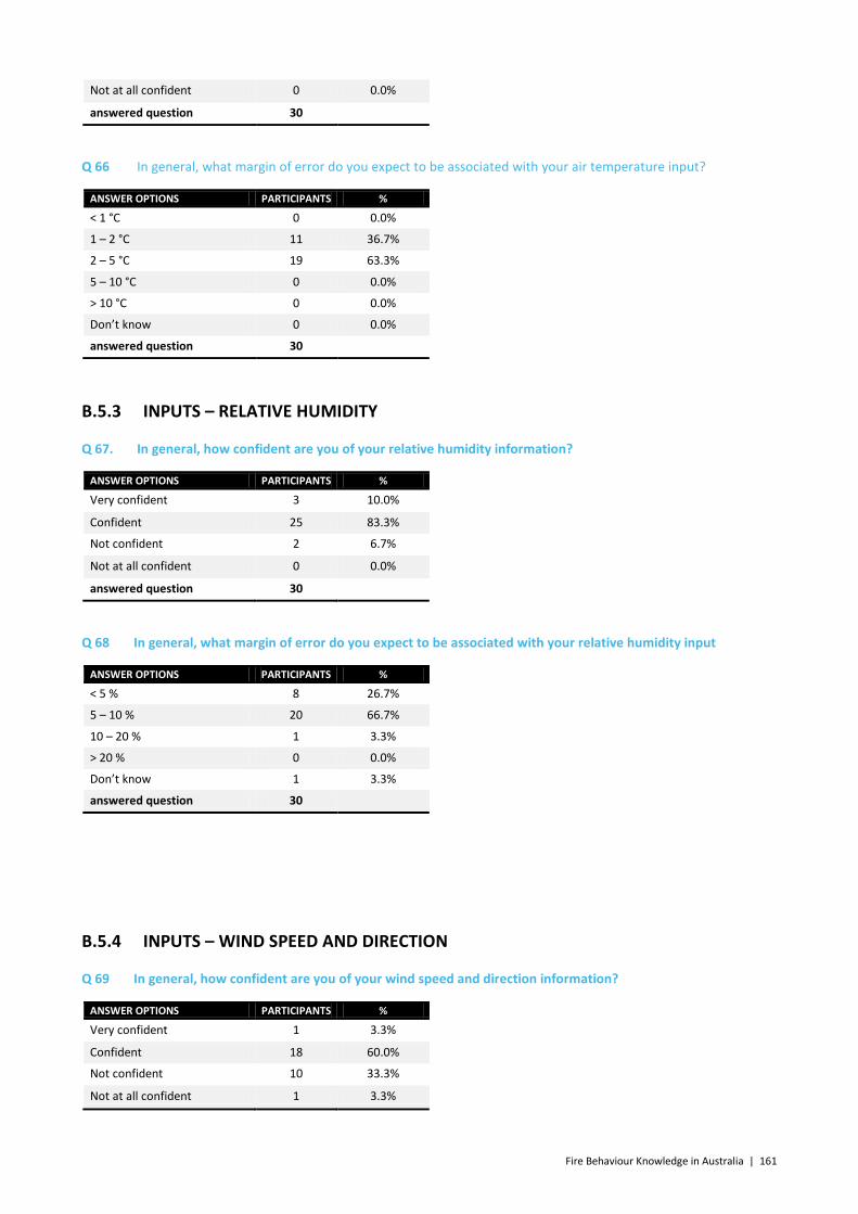
Fire Behaviour Knowledge in Australia | 161
Not at all confident 0 0.0%
answered question 30
Q 66 In general, what margin of error do you expect to be associated with your air temperature input?
ANSWER OPTIONS PARTICIPANTS %
< 1 °C 0 0.0%
1 – 2 °C 11 36.7%
2 – 5 °C 19 63.3%
5 – 10 °C 0 0.0%
> 10 °C 0 0.0%
Don’t know 0 0.0%
answered question 30
B.5.3 INPUTS – RELATIVE HUMIDITY
Q 67. In general, how confident are you of your relative humidity information?
ANSWER OPTIONS PARTICIPANTS %
Very confident 3 10.0%
Confident 25 83.3%
Not confident 2 6.7%
Not at all confident 0 0.0%
answered question 30
Q 68 In general, what margin of error do you expect to be associated with your relative humidity input
ANSWER OPTIONS PARTICIPANTS %
< 5 % 8 26.7%
5 – 10 % 20 66.7%
10 – 20 % 1 3.3%
> 20 % 0 0.0%
Don’t know 1 3.3%
answered question 30
B.5.4 INPUTS – WIND SPEED AND DIRECTION
Q 69 In general, how confident are you of your wind speed and direction information?
ANSWER OPTIONS PARTICIPANTS %
Very confident 1 3.3%
Confident 18 60.0%
Not confident 10 33.3%
Not at all confident 1 3.3%

162 | Fire Behaviour Knowledge in Australia
answered question 30
Q 70 In general, what margin of error do you expect to be associated with your wind speed input?
ANSWER OPTIONS PARTICIPANTS %
< 25 % 13 43.3%
25 – 50 % 16 53.3%
50 – 75 % 1 3.3%
75 – 100 % 0 0.0%
> 100 % 0 0.0%
Don’t know 0 0.0%
answered question 30
Q 71 In general, what margin of error do you expect to be associated with your wind direction input?
ANSWER OPTIONS PARTICIPANTS %
< 10 ° 5 16.7%
10 – 30 ° 24 80.0%
30 – 45 ° 0 0.0%
45 – 90 ° 1 3.3%
> 90 ° 0 0.0%
Don’t know 0 0.0%
answered question 30
Q 72 How often do the following effects require you to modify wind speed and direction?
ANSWER OPTIONS MOST OF THE TIME ALMOST ALWAYS SOMETIMES NEVER PARTICIPANTS
Topographic effects 14 6 10 0 30
46.7% 20.0% 33.3% 0.0%
Forest structure effects 9 9 12 0 30
30.0% 30.0% 40.0% 0.0%
Sea breeze 3 4 22 1 30
10.0% 13.3% 73.3% 3.3%
Fire effects 4 1 24 1 30
13.3% 3.3% 80.0% 3.3%
answered question 30
B.5.5 INPUTS – PRECIPITATION
Q 73 In general, how confident are you of your probability of precipitation information?
ANSWER OPTIONS PARTICIPANTS %
Very confident 2 6.7%
Confident 17 56.7%
Not confident 11 36.7%
Not at all confident 0 0.0%
answered question 30

Fire Behaviour Knowledge in Australia | 163
Q 74 In general, what margin of error do you expect to be associated with your timing of precipitation input? ANSWER OPTIONS PARTICIPANTS %
< 1 hour 1 3.3%
1 – 3 hours 19 63.3%
3 – 6 hours 6 20.0%
> 12 hours 2 6.7%
Don’t know 2 6.7%
answered question 30
Q 75 In general, what margin of error do you expect to be associated with your amount of precipitation input?
ANSWER OPTIONS PARTICIPANTS %
< 5 mm 11 36.7%
5 – 15 mm 18 60.0%
> 15 mm 0 0.0%
Don't know 1 3.3%
answered question 30
B.5.6 INPUTS – ATMOSPHERIC CONDITIONS
Q 76 How often do you use descriptions of the upper atmosphere condition?
MOST OF THE TIME ALMOST ALWAYS SOMETIMES NEVER PARTICIPANTS
F160 5 6 10 7 28
17.9% 21.4% 35.7% 25.0%
Haines/C-Haines 14 7 6 2 29
48.3% 24.1% 20.7% 6.9%
answered question 30
Q 77 If used, do you use it to: (select all that apply)
ANSWER OPTIONS PARTICIPANTS %
Modify the weather inputs 11 39.3%
Modify the fire model outputs 11 39.3%
Adjust the weather inputs for fires requiring multiple forecasts 9 32.1%
Adjust the fire model outputs for fires requiring multiple forecasts 5 17.9%
Other 13 46.4%
answered question 28
Develop confidence with prediction Having an understanding of the weather mixing down is central to being able to provide an accurate spread prediction. It's also useful for thinking about spot fire potential. Help assess risk of convective driven fires, to help assess stability. Fire model outputs are changed via changes to weather inputs Develop broader situation awareness and identify potential risk factors that may affect fire behaviour that may require weather inputs to be adjusted, or potential "blow-up" conditions to be anticipated and communicated Adjust weather inputs and fire model outputs, produce alternate weather stream from surface conditions with mixing down of upper level winds)
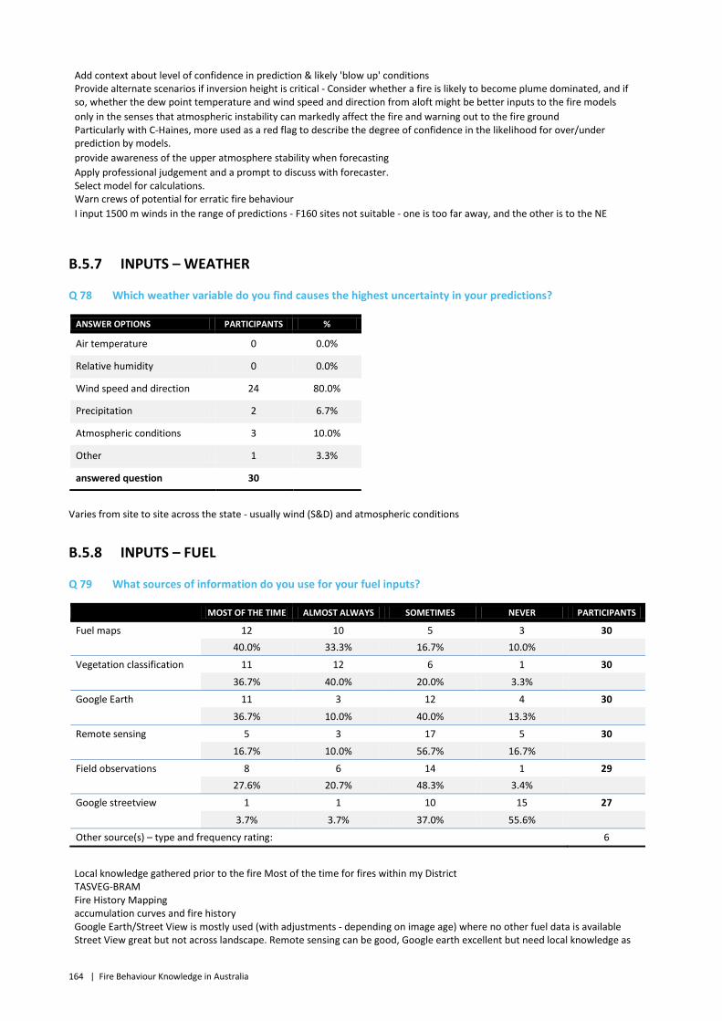
164 | Fire Behaviour Knowledge in Australia
Add context about level of confidence in prediction & likely 'blow up' conditions Provide alternate scenarios if inversion height is critical - Consider whether a fire is likely to become plume dominated, and if so, whether the dew point temperature and wind speed and direction from aloft might be better inputs to the fire models only in the senses that atmospheric instability can markedly affect the fire and warning out to the fire ground Particularly with C-Haines, more used as a red flag to describe the degree of confidence in the likelihood for over/under prediction by models. provide awareness of the upper atmosphere stability when forecasting Apply professional judgement and a prompt to discuss with forecaster. Select model for calculations. Warn crews of potential for erratic fire behaviour I input 1500 m winds in the range of predictions - F160 sites not suitable - one is too far away, and the other is to the NE
B.5.7 INPUTS – WEATHER
Q 78 Which weather variable do you find causes the highest uncertainty in your predictions?
ANSWER OPTIONS PARTICIPANTS %
Air temperature 0 0.0%
Relative humidity 0 0.0%
Wind speed and direction 24 80.0%
Precipitation 2 6.7%
Atmospheric conditions 3 10.0%
Other 1 3.3%
answered question 30
Varies from site to site across the state - usually wind (S&D) and atmospheric conditions
B.5.8 INPUTS – FUEL
Q 79 What sources of information do you use for your fuel inputs?
MOST OF THE TIME ALMOST ALWAYS SOMETIMES NEVER PARTICIPANTS
Fuel maps 12 10 5 3 30 40.0% 33.3% 16.7% 10.0%
Vegetation classification 11 12 6 1 30
36.7% 40.0% 20.0% 3.3%
Google Earth 11 3 12 4 30
36.7% 10.0% 40.0% 13.3%
Remote sensing 5 3 17 5 30
16.7% 10.0% 56.7% 16.7%
Field observations 8 6 14 1 29 27.6% 20.7% 48.3% 3.4%
Google streetview 1 1 10 15 27
3.7% 3.7% 37.0% 55.6%
Other source(s) – type and frequency rating: 6
Local knowledge gathered prior to the fire Most of the time for fires within my District TASVEG-BRAM Fire History Mapping accumulation curves and fire history Google Earth/Street View is mostly used (with adjustments - depending on image age) where no other fuel data is available Street View great but not across landscape. Remote sensing can be good, Google earth excellent but need local knowledge as
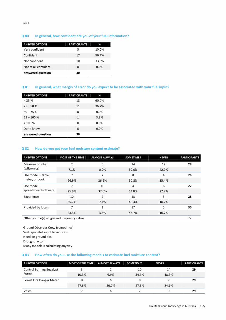
Fire Behaviour Knowledge in Australia | 165
well
Q 80 In general, how confident are you of your fuel information?
ANSWER OPTIONS PARTICIPANTS %
Very confident 3 10.0%
Confident 17 56.7%
Not confident 10 33.3%
Not at all confident 0 0.0%
answered question 30
Q 81 In general, what margin of error do you expect to be associated with your fuel input?
ANSWER OPTIONS PARTICIPANTS %
< 25 % 18 60.0%
25 – 50 % 11 36.7%
50 – 75 % 0 0.0%
75 – 100 % 1 3.3%
> 100 % 0 0.0%
Don’t know 0 0.0%
answered question 30
Q 82 How do you get your fuel moisture content estimate?
ANSWER OPTIONS MOST OF THE TIME ALMOST ALWAYS SOMETIMES NEVER PARTICIPANTS
Measure on site (wiltronics)
2 0 14 12 28
7.1% 0.0% 50.0% 42.9%
Use model – table, meter, or book
7 7 8 4 26
26.9% 26.9% 30.8% 15.4%
Use model –spreadsheet/software
7 10 4 6 27 25.9% 37.0% 14.8% 22.2%
Experience 10 2 13 3 28 35.7% 7.1% 46.4% 10.7%
Provided by locals 7 1 17 5 30
23.3% 3.3% 56.7% 16.7%
Other source(s) – type and frequency rating: 5
Ground Observer Crew (sometimes) Seek specialist input from locals Need on ground obs Drought factor Many models is calculating anyway
Q 83 How often do you use the following models to estimate fuel moisture content?
ANSWER OPTIONS MOST OF THE TIME ALMOST ALWAYS SOMETIMES NEVER PARTICIPANTS
Control Burning Eucalypt Forest
3 2 10 14 29 10.3% 6.9% 34.5% 48.3%
Forest Fire Danger Meter 8 6 8 7 29
27.6% 20.7% 27.6% 24.1%
Vesta 7 6 7 9 29
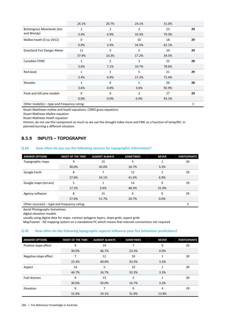
166 | Fire Behaviour Knowledge in Australia
24.1% 20.7% 24.1% 31.0%
Buttongrass Moorlands (Jon and Wendy)
1 2 3 23 29 3.4% 6.9% 10.3% 79.3%
Mallee-heath (Cruz 2012) 0 1 10 18 29 0.0% 3.4% 34.5% 62.1%
Grassland Fire Danger Meter 11 3 5 10 29 37.9% 10.3% 17.2% 34.5%
Canadian FFMC 1 2 3 22 28
3.6% 7.1% 10.7% 78.6%
Red book 1 2 5 21 29
3.4% 6.9% 17.2% 72.4%
Sharples 1 0 1 26 28 3.6% 0.0% 3.6% 92.9%
Pook and Gill pine models 0 0 2 27 29 0.0% 0.0% 6.9% 93.1%
Other model(s) – type and frequency rating: 3
Stuart Matthews mallee and heath equations. CSIRO grass equations Stuart Mathews Mallee equation Stuart Mathews Heath equation Hmmm, do not use this component as much as we use the drought index more and FMC as a function of temp/RH. in planned burning a different situation
B.5.9 INPUTS – TOPOGRAPHY
Q 84 How often do you use the following sources for topographic information?
ANSWER OPTIONS MOST OF THE TIME ALMOST ALWAYS SOMETIMES NEVER PARTICIPANTS
Topographic maps 9 15 5 1 30 30.0% 50.0% 16.7% 3.3%
Google Earth 8 7 12 2 29 27.6% 24.1% 41.4% 6.9%
Google maps (terrain) 5 1 14 9 29 17.2% 3.4% 48.3% 31.0%
Agency software 8 15 6 0 29 27.6% 51.7% 20.7% 0.0%
Other source(s) – type and frequency rating: 3 Aerial Photographs Sometimes digital elevation models usually using digital data for maps- contour polygons layers, slope grids, aspect grids MapToaster - NZ mapping system on a standalone PC which means that internet connections not required
Q 85 How often do the following topographic aspects influence your fire behaviour predictions?
ANSWER OPTIONS MOST OF THE TIME ALMOST ALWAYS SOMETIMES NEVER PARTICIPANTS
Positive slope effect 9 14 7 0 30
30.0% 46.7% 23.3% 0.0%
Negative slope effect 7 12 10 1 30
23.3% 40.0% 33.3% 3.3%
Aspect 14 5 10 1 30 46.7% 16.7% 33.3% 3.3%
Fuel dryness 9 15 5 1 30 30.0% 50.0% 16.7% 3.3%
Elevation 9 7 9 4 29 31.0% 24.1% 31.0% 13.8%
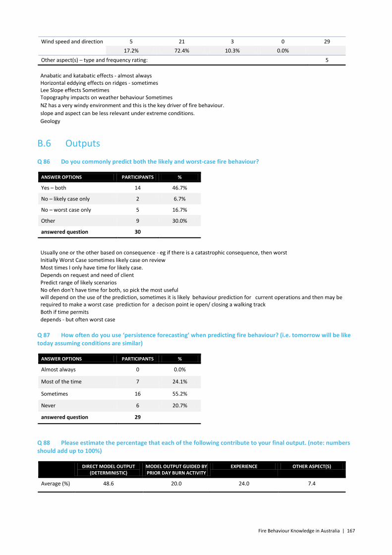
Fire Behaviour Knowledge in Australia | 167
Wind speed and direction 5 21 3 0 29 17.2% 72.4% 10.3% 0.0%
Other aspect(s) – type and frequency rating: 5
Anabatic and katabatic effects - almost always Horizontal eddying effects on ridges - sometimes Lee Slope effects Sometimes Topography impacts on weather behaviour Sometimes NZ has a very windy environment and this is the key driver of fire behaviour. slope and aspect can be less relevant under extreme conditions. Geology
B.6 Outputs
Q 86 Do you commonly predict both the likely and worst-case fire behaviour?
ANSWER OPTIONS PARTICIPANTS %
Yes – both 14 46.7%
No – likely case only 2 6.7%
No – worst case only 5 16.7%
Other 9 30.0%
answered question 30
Usually one or the other based on consequence - eg if there is a catastrophic consequence, then worst Initially Worst Case sometimes likely case on review Most times I only have time for likely case. Depends on request and need of client Predict range of likely scenarios No ofen don't have time for both, so pick the most useful will depend on the use of the prediction, sometimes it is likely behaviour prediction for current operations and then may be required to make a worst case prediction for a decison point ie open/ closing a walking track Both if time permits depends - but often worst case
Q 87 How often do you use ‘persistence forecasting’ when predicting fire behaviour? (i.e. tomorrow will be like today assuming conditions are similar)
ANSWER OPTIONS PARTICIPANTS %
Almost always 0 0.0%
Most of the time 7 24.1%
Sometimes 16 55.2%
Never 6 20.7%
answered question 29
Q 88 Please estimate the percentage that each of the following contribute to your final output. (note: numbers should add up to 100%)
DIRECT MODEL OUTPUT (DETERMINISTIC)
MODEL OUTPUT GUIDED BY PRIOR DAY BURN ACTIVITY
EXPERIENCE OTHER ASPECT(S)
Average (%) 48.6 20.0 24.0 7.4
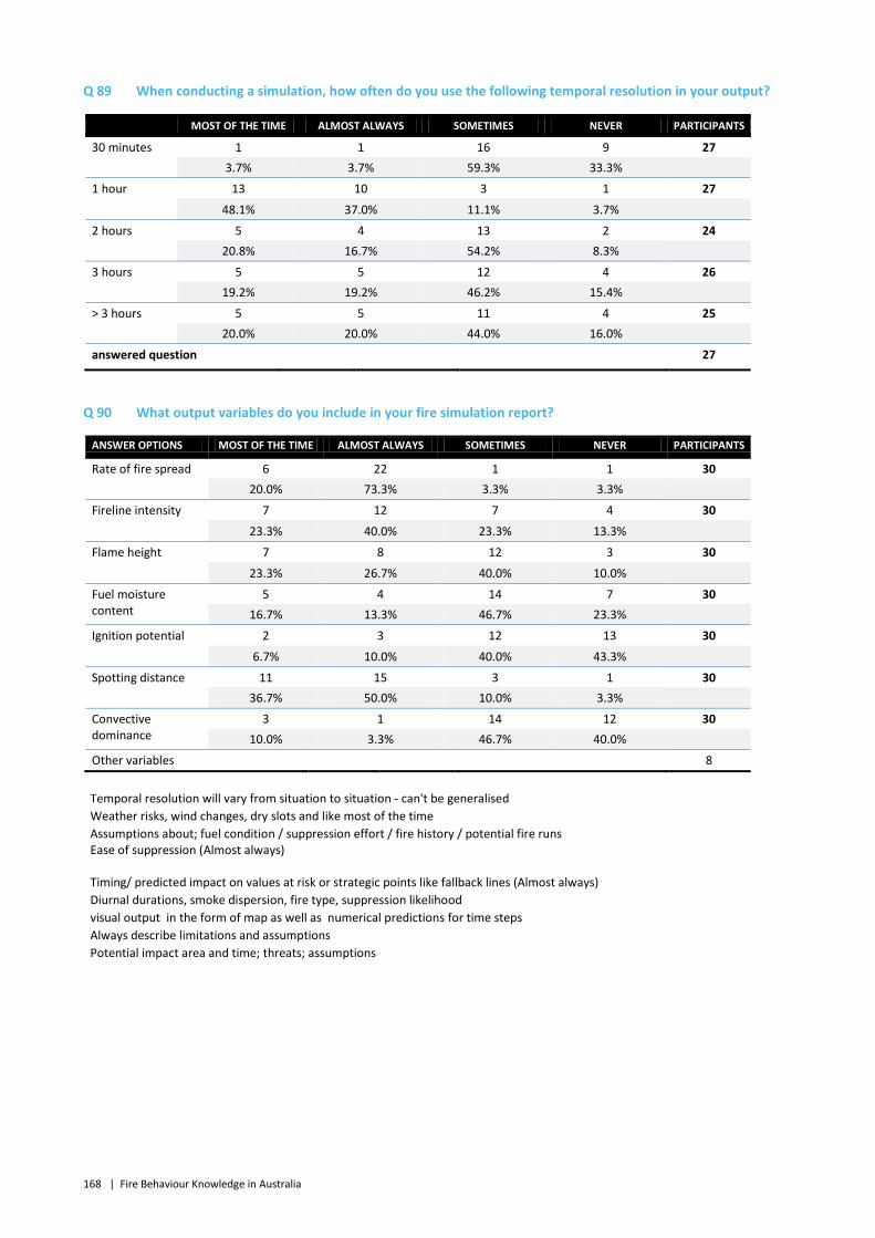
168 | Fire Behaviour Knowledge in Australia
Q 89 When conducting a simulation, how often do you use the following temporal resolution in your output?
MOST OF THE TIME ALMOST ALWAYS SOMETIMES NEVER PARTICIPANTS
30 minutes 1 1 16 9 27 3.7% 3.7% 59.3% 33.3%
1 hour 13 10 3 1 27
48.1% 37.0% 11.1% 3.7%
2 hours 5 4 13 2 24 20.8% 16.7% 54.2% 8.3%
3 hours 5 5 12 4 26 19.2% 19.2% 46.2% 15.4%
> 3 hours 5 5 11 4 25 20.0% 20.0% 44.0% 16.0%
answered question 27
Q 90 What output variables do you include in your fire simulation report?
ANSWER OPTIONS MOST OF THE TIME ALMOST ALWAYS SOMETIMES NEVER PARTICIPANTS
Rate of fire spread 6 22 1 1 30 20.0% 73.3% 3.3% 3.3%
Fireline intensity 7 12 7 4 30
23.3% 40.0% 23.3% 13.3%
Flame height 7 8 12 3 30
23.3% 26.7% 40.0% 10.0%
Fuel moisture content
5 4 14 7 30 16.7% 13.3% 46.7% 23.3%
Ignition potential 2 3 12 13 30
6.7% 10.0% 40.0% 43.3%
Spotting distance 11 15 3 1 30 36.7% 50.0% 10.0% 3.3%
Convective dominance
3 1 14 12 30 10.0% 3.3% 46.7% 40.0%
Other variables 8
Temporal resolution will vary from situation to situation - can't be generalised Weather risks, wind changes, dry slots and like most of the time Assumptions about; fuel condition / suppression effort / fire history / potential fire runs Ease of suppression (Almost always) Timing/ predicted impact on values at risk or strategic points like fallback lines (Almost always) Diurnal durations, smoke dispersion, fire type, suppression likelihood visual output in the form of map as well as numerical predictions for time steps Always describe limitations and assumptions Potential impact area and time; threats; assumptions
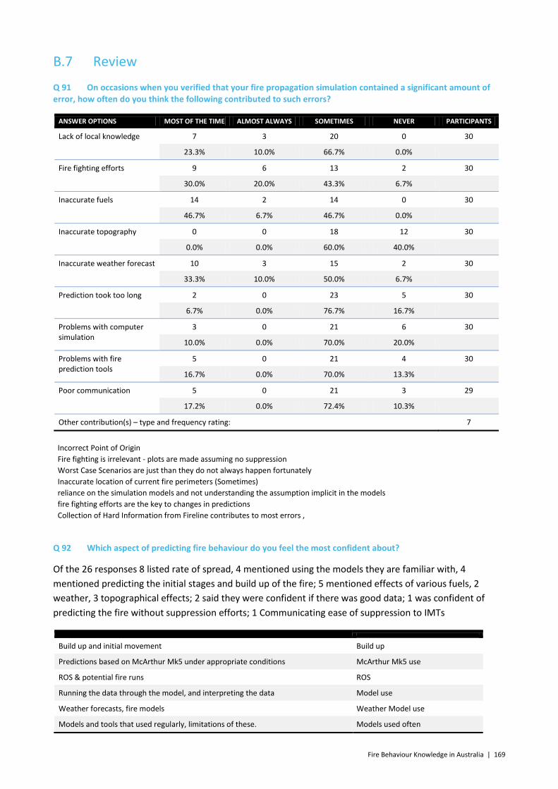
Fire Behaviour Knowledge in Australia | 169
B.7 Review
Q 91 On occasions when you verified that your fire propagation simulation contained a significant amount of error, how often do you think the following contributed to such errors?
ANSWER OPTIONS MOST OF THE TIME ALMOST ALWAYS SOMETIMES NEVER PARTICIPANTS
Lack of local knowledge 7 3 20 0 30
23.3% 10.0% 66.7% 0.0%
Fire fighting efforts 9 6 13 2 30
30.0% 20.0% 43.3% 6.7%
Inaccurate fuels 14 2 14 0 30
46.7% 6.7% 46.7% 0.0%
Inaccurate topography 0 0 18 12 30
0.0% 0.0% 60.0% 40.0%
Inaccurate weather forecast 10 3 15 2 30
33.3% 10.0% 50.0% 6.7%
Prediction took too long 2 0 23 5 30
6.7% 0.0% 76.7% 16.7%
Problems with computer simulation
3 0 21 6 30
10.0% 0.0% 70.0% 20.0%
Problems with fire prediction tools
5 0 21 4 30
16.7% 0.0% 70.0% 13.3%
Poor communication 5 0 21 3 29
17.2% 0.0% 72.4% 10.3%
Other contribution(s) – type and frequency rating: 7
Incorrect Point of Origin Fire fighting is irrelevant - plots are made assuming no suppression Worst Case Scenarios are just than they do not always happen fortunately Inaccurate location of current fire perimeters (Sometimes) reliance on the simulation models and not understanding the assumption implicit in the models fire fighting efforts are the key to changes in predictions Collection of Hard Information from Fireline contributes to most errors ,
Q 92 Which aspect of predicting fire behaviour do you feel the most confident about?
Of the 26 responses 8 listed rate of spread, 4 mentioned using the models they are familiar with, 4 mentioned predicting the initial stages and build up of the fire; 5 mentioned effects of various fuels, 2 weather, 3 topographical effects; 2 said they were confident if there was good data; 1 was confident of predicting the fire without suppression efforts; 1 Communicating ease of suppression to IMTs
Build up and initial movement Build up
Predictions based on McArthur Mk5 under appropriate conditions McArthur Mk5 use
ROS & potential fire runs ROS
Running the data through the model, and interpreting the data Model use
Weather forecasts, fire models Weather Model use
Models and tools that used regularly, limitations of these. Models used often
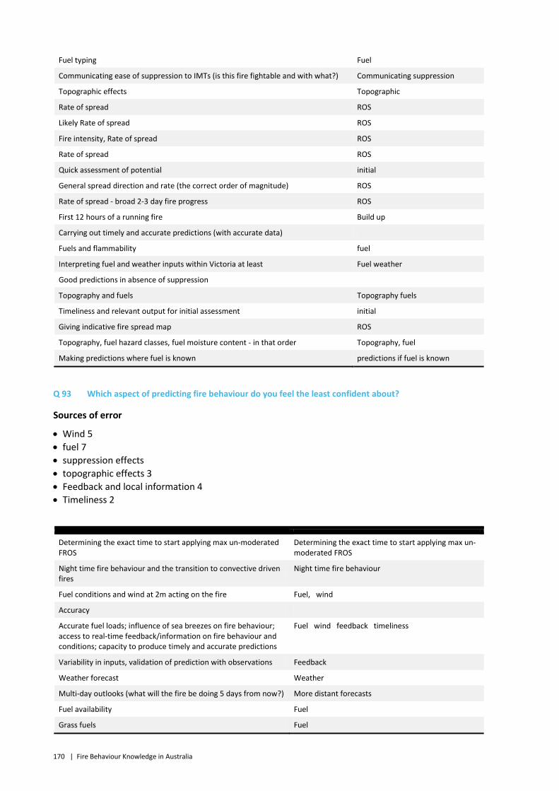
170 | Fire Behaviour Knowledge in Australia
Fuel typing Fuel
Communicating ease of suppression to IMTs (is this fire fightable and with what?) Communicating suppression
Topographic effects Topographic
Rate of spread ROS
Likely Rate of spread ROS
Fire intensity, Rate of spread ROS
Rate of spread ROS
Quick assessment of potential initial
General spread direction and rate (the correct order of magnitude) ROS
Rate of spread - broad 2-3 day fire progress ROS
First 12 hours of a running fire Build up
Carrying out timely and accurate predictions (with accurate data)
Fuels and flammability fuel
Interpreting fuel and weather inputs within Victoria at least Fuel weather
Good predictions in absence of suppression
Topography and fuels Topography fuels
Timeliness and relevant output for initial assessment initial
Giving indicative fire spread map ROS
Topography, fuel hazard classes, fuel moisture content - in that order Topography, fuel
Making predictions where fuel is known predictions if fuel is known
Q 93 Which aspect of predicting fire behaviour do you feel the least confident about?
Sources of error
• Wind 5 • fuel 7 • suppression effects • topographic effects 3 • Feedback and local information 4 • Timeliness 2
Determining the exact time to start applying max un-moderated FROS
Determining the exact time to start applying max un-moderated FROS
Night time fire behaviour and the transition to convective driven fires
Night time fire behaviour
Fuel conditions and wind at 2m acting on the fire Fuel, wind
Accuracy
Accurate fuel loads; influence of sea breezes on fire behaviour; access to real-time feedback/information on fire behaviour and conditions; capacity to produce timely and accurate predictions
Fuel wind feedback timeliness
Variability in inputs, validation of prediction with observations Feedback
Weather forecast Weather
Multi-day outlooks (what will the fire be doing 5 days from now?) More distant forecasts
Fuel availability Fuel
Grass fuels Fuel
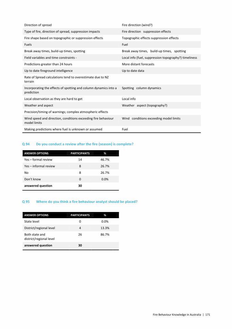
Fire Behaviour Knowledge in Australia | 171
Direction of spread Fire direction (wind?)
Type of fire, direction of spread, suppression impacts Fire direction suppression effects
Fire shape based on topographic or suppression effects Topographic effects suppression effects
Fuels Fuel
Break away times, build-up times, spotting Break away times, build-up times, spotting
Field variables and time constraints - Local info (fuel, suppression topography?) timeliness
Predictions greater than 24 hours More distant forecasts
Up to date fireground intelligence Up to date data
Rate of Spread calculations tend to overestimate due to NZ terrain
Incorporating the effects of spotting and column dynamics into a prediction
Spotting column dynamics
Local observation as they are hard to get Local info
Weather and aspect Weather aspect (topography?)
Precision/timing of warnings; complex atmospheric effects
Wind speed and direction, conditions exceeding fire behaviour model limits
Wind conditions exceeding model limits
Making predictions where fuel is unknown or assumed Fuel
Q 94 Do you conduct a review after the fire (season) is complete?
ANSWER OPTIONS PARTICIPANTS %
Yes – formal review 14 46.7%
Yes – informal review 8 26.7%
No 8 26.7%
Don’t know 0 0.0%
answered question 30
Q 95 Where do you think a fire behaviour analyst should be placed?
ANSWER OPTIONS PARTICIPANTS %
State level 0 0.0%
District/regional level 4 13.3%
Both state and district/regional level
26 86.7%
answered question 30

FOR FURTHER INFORMATION
Ecosystem Sciences/Digital Productivity and Services
Andrew Sullivan
t +61 2 6246 4051
w www.csiro.au