Finite element simulation of metal forming processes inABAQUSYang, J.; Technische Universiteit Eindhoven (TUE). Stan Ackermans Instituut.Computergesteund ontwerpen en fabriceren van discrete produkten

Published: 01/01/1992

Document VersionPublisher’s PDF, also known as Version of Record (includes final page, issue and volume numbers)

Please check the document version of this publication:

• A submitted manuscript is the author's version of the article upon submission and before peer-review. There can be important differencesbetween the submitted version and the official published version of record. People interested in the research are advised to contact theauthor for the final version of the publication, or visit the DOI to the publisher's website.• The final author version and the galley proof are versions of the publication after peer review.• The final published version features the final layout of the paper including the volume, issue and page numbers.

Link to publication

Citation for published version (APA):Yang, J., & Technische Universiteit Eindhoven (TUE). Stan Ackermans Instituut. Computergesteund ontwerpenen fabriceren van discrete produkten (1992). Finite element simulation of metal forming processes in ABAQUSEindhoven: Technische Universiteit Eindhoven

General rightsCopyright and moral rights for the publications made accessible in the public portal are retained by the authors and/or other copyright ownersand it is a condition of accessing publications that users recognise and abide by the legal requirements associated with these rights.

• Users may download and print one copy of any publication from the public portal for the purpose of private study or research. • You may not further distribute the material or use it for any profit-making activity or commercial gain • You may freely distribute the URL identifying the publication in the public portal ?

Take down policyIf you believe that this document breaches copyright please contact us providing details, and we will remove access to the work immediatelyand investigate your claim.

Download date: 29. May. 2018

Computer Aided Design and Manufacture

of Discrete Products

FINITE ELEMENT SIMULATION OF METALFORMING PROCESSES IN ABAQUS

Jing Han YANG

SUMMARY

The finite element simulation of metal forming processes is very

useful to predict the strain, stress, working force and ductile

failure. Ductile failure is defined as the initiation of cracks

during the plastic deformation. It delimits the maximal possible

deformation in forming processes.

As an example to test the ductile failure idea, the finite element

simulation of a metal forming process was made in ABAQUS. Although

the simulation of this kind of problem is successful, some

inherent defects of ABAQUS are found. Finally some proposals to

overcome these defects are presented.

If only the effect of stress state is accounted for, an attractive

way to represent material ductility is the failure curve. It gives

the triaxiality (Um/Uf) versus the equivalent strain e at ductile

failure. The triaxiality is the quotient of the hydrostatic stress

and the flow stress. A failure curve is obtained in general by

the torsion and tensile tests of cylindrical specimens. In the

course of a tensile test the occurrence of necking introduces a

triaxial stress state.

Of known models, besides finite element models, the Bridgman model

is suitable to describe the stress state during necking, but its

accuracy has to be doubted [ 15]. Finite element models are the

most accurate, but a computer system and complex programs are

needed. This makes them less suitable for practice in some cases.

The application of the Bridgman model therefore is still of

importance in practice. But its accuracy must be verified.

In this thesis the tensile test simUlation in ABAQUS is performed.

Two groups of results of the triaxiality and strain are compared

for investigating the correctness of the Bridgman model. Results

indicate that the Bridgman model has a better agreement with

finite element model with the increase of the strain hardening

exponent n, but a correction parameter, which should be put in the

CONTENTS

2.1 Nonlinear solution methods

2.2 Basic finite element equation

3 FINITE ELEMENT SIMULATION OF BACKWARD CAN EXTRUSION

SUMMARY

1 INTRODUCTION

2 BASIC ALGORITHM AND BASIC EQUATION IN ABAQUS

3.6.1 Deformed mesh

3.6.2 Equivalent stress and strain

3.6.3 Extrusion force

3.6.4 Triaxiality

4 FINITE ELEMENT SIMULATION OF THE TENSILE TEST

48

50

52

53

55

1

5

5

8

15

15

16

16

18

21

23

26

27

27

29

31

33

34

34

35

36

36

37

39

41

Finite element model

The selection of elements

Four node solid isoparametric element

Interface element and rigid surface

static analysis

constitutive relationship

Mesh rezoning

Results and discussion

4.1

4.2

4.3

4.3.1

4.3.2

4.3.3

4.3.4

4.3.5

3.1

3.2

3.2.1

3.2.2

3.3

3.4

3.5

3.6

Finite element model

Bridgman model

Results and discussion

The finite element meshes of the necking process

Equivalent strain

Triaxiality

The curves of the triaxiality versus the strain

The comparison of the ABAQUS solution

and the MARC solution of triaxiality

5 CONCLUSIONS

ACKNOWLEDGEMENT

REFERENCES

APPENDIX A INPUT FILES

A.1

A.2

The input file of the backward

can extrusion problem

The input file of the tensile test problem

55

59

APPENDIX B DEFORMED MESHES, COI\ITOUR PLOTS OF

EQUIVALENT STRAIN AND TRIAXIALITY

B.l

B.2

strain hardening exponent n=O.OO

strain hardening exponent n=O.28

65

65

68

1 INTRODUCTION

A significant advantage in the field of Computer Aided Design and

Manufacture of Discrete Products is that the time from design to

manufacture can be shortened greatly. But to complete this process

many problems must be solved.

One of the problems to shorten the time from design to production

for the market is the lack of knowledge of the designer in the

field of the combination of material and mechanical forming

technology. When someone designs a part of a product, he has to

know not only that it can be made by a mechanical working process

but also his material choice is suitable for this process. In many

cases, the constraints of a material for a given process are given

by its ductility.

Ductility can be regarded as a material characteristic that

describes the response of a material to the process parameters,

with respect to ductile failure. If only the effect of the state

of stress has to be accounted for, an attractive way to represent

this characteristic is a curve, which is called failure curve. It

gives the triaxiality (Um/Uf') versus the equivalent strain Cf' at

ductile failure. In this relation Um is the hydrostatic stress and

Uf' the flow stress of the material.

Ductile failure, being the initiation of cracks during plastic

deformation, is a phenomenon of considerable importance in the

field of metal working. It may limit the formability of a metal in

forming processes, while it may be the condition for the

separation, that occurs in separating processes such as in

punching or cutting.

An effective method to predict ductile failure is the finite

element simulation of metal forming processes under the condition

that the equivalent strain and triaxiality at ductile failure is

known. In general, the curves of the triaxiality versus the

equivalent strain are obtained by the tensile and torsion tests of

1

cylindrical bars.

In this thesis, the basic algorithm and equilibrium equation in

ABAQUS [13] are first described simply in Chapter 2, and then two

calculations in ABAQUS, the finite element simulation of backward

can extrusion and the finite element simulation of the tensile

test, are introduced and analyzed in Chapter 3 and in Chapter 4

respectively.

Large elastic-plastic deformation processes are characterized by

severe nonlinear material and geometric behavior. As a consequence

both have to be taken into account.

In general, the nonlinear problems were treated as an extension of

linear structural problems and the application was confined to

deformation where the plastic strain was of the order of a few

percent. However, for metal forming operations such a structural

approach does hardly make sense. Here it is actually the objective

to change the geometry drastically. In the numerical analysis it

is necessary to discretize the deformation history. This requires

a sequential incremental analysis of the continuously deforming

body.

Regarding the state of a deformed body two descriptions are

possible, which are dependent on the definition of the reference

frame in which the deformation is described. The Lagrange method

[1] is based on a material-bounded coordinate system, whereas in

the Euler method [1] the deformation are referred to a fixed

special coordinate system. The kinematic relations for a deforming

body are most easily expressed by employing the Lagrange type of

formulations, whereas the rheological approach of plasticity

commends to an Euler formulation.

An approach in which the advantages of both methods are retained

was pioneered by McMeeking and Rice (1975) [2]. They used an

updated Lagrange formulation in which each incremental step of the

calculation is based upon an update reference state. Following

2

this approach it has become possible to get the steady state of a

metal forming process at the termination of a transient

elastic-plastic flow through successive deformation stages. The

updated Lagrange method is used in ABAQUS owing to its suitability

for the analysis of metal forming processes.

The strong element mesh distortion during continuously increasing

deformation is inherent to the updated Lagrange formulation. Most

of the computations must be stopped prematurely, because the

results in the distorted elements become unreliable. Proceeding

those calculations is even impossible owing to mesh degeneration.

Therefore, the mesh must be rezoned before the mesh distortion

occurs. ABAQUS offers the function of rezoning the mesh. This

technique makes it possible to redefine an element mesh at regular

intervals on the basis of the deformation and to continue the

computation of large deformation.

The finite element simulation of backward can extrusion is very

useful to predict the punch force, strain, stress and possible

fracture etc. in metal forming processes.

Some authors have used finite elements to simulate the deformation

of backward can extrusion in some finite element programs such as

P. Hartley [3] [4]. He used the program MAFEPM 111 developed by P.

Hartley in 1977 and also the program EPFEPM [5] by means of which

the eight node elements were used and the mesh was rezoned on a

microcomputer system. C. J. M. Gelten [6] used the program MARC by

means of which the mesh can be rezoned automatically. J. S. Park

[7] also presented a method of automatic remeshing and applied the

method to the problem of backward can extrusion. But up to now,

the paper which describes the finite element simulation of

backward can extrusion in ABAQUS has not been found. In this

thesis, some main options combined with the descriptions of

theory and option principles are introduced and some defects in

comparison with other programs are discussed and the results are

analyzed.

3

In a tensile test, failure usually is preceded by a localized

reduction in diameter called necking. The formation of a neck

introduces a triaxial state of stress in this region. Here,

continued deformation starts nucleated voids in this region to

grow and coalescence, and finally initiate a crack. This crack

starts in the centre of the smallest cross section of the

specimen. Therefore, the state of stress and strain in the middle

of the smallest cross section of a tensile test specimen are of

great interest to us. These local quantities cannot be measured

directly, therefore models describing these have to be employed. A

well-known analytical model, describing the situation mentioned

above, is the model developed by Bridgman (1952) [8]. This model

assumes the equivalent strain across the smallest cross section to

be constant. From a practical point of view, the Bridgman model is

the most suitable to use in practice because of its simplicity.

its accuracy, however, has to be doubted. Finite element models

are believed to be more accurate, but a computer and complex

programs are needed. This makes them less suitable for practice.

Therefore, the Bridgman model must be verified in finite element

model for practical use.

In the second calculation, the tensile test simulation in ABAQUS

is performed. Two groups of results of the triaxiality and strain

are compared for investigating the correctness of the Bridgman

model. One group of results is taken from the finite element model

directly. Another group of results is obtained using the Bridgman

model in which the required data also are taken from the same

finite element model, such as the radius of the smallest cross

section and the radius of profile arc during necking. Finally from

the description of the curves of the triaxiality (Um/U) versus the

equivalent strain e or the mean strain Cave and the mean strain

Cave versus the equivalent strain e, the difference between the

finite element solution and the Bridgman model solution is found.

On the basis of the results, some discussion points and proposals

will be given.

4

2 BASIC ALGORITHM AND BASIC EQUATION IN ABAQUS

The finite element model generated in ABAQUS [13] is usually

non-linear and may involve from a few to many thousand variables.

In terms of these variables, the equilibrium equations obtained by

discretizing the virtual work equation may be written sYmbolically

as

(2-1)

where ~ is the force component conjugate to the Nth variable in

the problem, and UK is the value of the Mth variable. The basic

problem is to solve Equation 2-1 for the UK throughout the history

of interest. Many of the problems to which ABAQUS will be applied

are history dependent, so the solution must be developed by a

series of small increments.

2.1 Nonlinear solution methods

ABAQUS generally used Newton's method as a numerical technique for

solving the nonlinear equilibrium equations. The basic formalism

of Newton's method is as follows. Assume that, after an iteration

i, an approximation UN, to the solution has been obtained. Let1

eN be the difference between this solution and the exact1+1

solution to the discrete equilibrium equation, Equation 2-1. This

means that

::If -K -K.1'" (u +c ) =0.

1 1+1

Expanding the left-hand side of this equation

about the approximate solution UK and taking1

linear system of equations are obtained, i.e.

:-.NP-P -N.K C =-F.

1 1+1 1

where

5

in a Taylor series

first two terms, a

(2.1-1)

-N:-.NP aF -K.K =-- (u )

1 -p 1au

is the Jacobian matrix, and

Then

-K -K-KU =u +c

1+1 1 1+1

is the next approximation to the solution, and the iteration

continues.

Convergence of Newton's method is best measured by ensuring that

all entries in FN and all entries in cl are sUfficiently small.1 1+1

In ABAQUS, only the FN are checked against user prescribed force1

and moment tolerances (PTOL and MTOL), typical values being 0.1%

to 10% of actual loads.

The principal advantage of Newton's method is its quadratic

convergence rate. But the method has two major disadvantages: the

Jacobian matrix has to be calculated, and this same matrix has to

be solved. The most commonly used alternative to Newton is the

modified Newton method, in which the Jacobian in Equation 2.1-1 is

only recalculate occasionally (or not at all, as in the initial

strain method of simple contained plasticity problem). This method

is attractive for mildly nonlinear problems involving softening

behavior (such as contained plasticity with monotonic straining),

but is not suitable for more severely nonlinear cases. Another

alternate is the quasi-Newton method in which the inverse Jacobian

is obtained by an iteration process. ABAQUS offers the "BFGS"

quasi-Newton method. Its convergence rate is slower than the

quadratic convergence rate of Newton's method, faster than the

convergence rate of the modified Newton method.

When any iterative algorithm is applied to a history dependent

6

problem the intermediate, nonconverged solutions obtained during

the iteration process are usually not on the actual solution path,

and thus the integration of history dependent variables must be

performed completely over the increment at each iteration, and not

obtained as the sum of integrations associated with each Newton

iteration, c. In ABAQUS, this is done by assuming that the basic1

nodal variables, u, vary linearly over the increment, so that

- ,; - ,;-u(';)=(l- f1t )U(l)+ f1t U(l+f1l),

where O::5,;::5f1t represents "time" during the increment. Then, for any

history dependent variable, g(t), we compute

at each iteration.

ABAQUS provides both "automatic" time step choice, as well as

direct user control, for all classes of problem. Direct user

control may be useful in cases where the problem behavior is well

understood, or in cases where the automatic algorithm do not

handle the problem well. However, the automatic schemes in the

program are based on extensive experience with a wide range of

problems, and therefore generally provide a reliable approach.

For static problems, ABAQUS uses a scheme based on the maximum

force residuals following each iteration. By comparing consecutive

values of these quantities, ABAQUS determines whether convergence

is likely in the number of iterations allowed by the analyst. If

convergence is deemed unlikely, ABAQUS adjusts the load increment;

if convergence is deemed likely and more iterations than allowed

by the user are needed, ABAQUS overrides the analyst's upper bound

on iterations (for this increment only). In this way, excessive

iteration is eliminated in cases where convergence is unlikely,

and an increment that appears to be converging is not aborted due

to its needing a few more iterations. One other ingredient in this

algorithm is that a minimum increment size is specified. This

7

prevents excessive computation in cases where buckling, limit

load, some modeling error causes the solution to stall. This

control is handled internally, with user override if needed.

Several other controls are built into the algorithm: for example,

it will cut back the increment size if an element inverts due to

excessively large geometry changes. These detailed controls are

based on empirical testing.

2.2 Basic finite element equation

Many of the problems to which ABAQUS is applied involved finding

an approximate finite element solution for the displacements,

deformations, stresses, and forces. The exact solution of such a

problem requires that both force and moment equilibrium be

maintained at all times over any arbitrary volume of body. the

displacement finite element method is based on approximating this

equilibrium requirement by replacing it with a weaker requirement,

that equilibrium must be maintained in an average sense over a

finite number of divisions of the volume of the body. In this

section, the exact equilibrium statement is first written in the

form of the virtual work statement and then the approximate form

of equilibrium used in a finite element model is derived.

Let V denote a volume occupied by a part of the body in the

current configuration and let S be the surface bounding this

volume. Let the surface traction at any point on S be the force t

per unit of current area, and let the body force at any point

within the volume of material under consideration be f per unit of

current volume. Then force equilibrium for the volume is

I tds+I fdV=Os v

(2.2-1)

-The "true" or Cauchy stress matrix (J" at a point of S is defined by

- -t=no(J" (2.2-2)

-where n is the unit outward normal to S at the point. Using this

8

this equation must apply point wise

the differential equation of

definition, Equation 2.2-2 is

J lioUdS+J fdV=Os v

Gauss' theorem allows us to rewrite a surface integral as a volume

integral according to

J lio( )dS=J ~x ( ) dVs . v

where ( is any continuous function-scalar vector or tensor.

Applying the Gauss theorem to the surface integral in the

equilibrium equation gives

J- - J anoudS= (ax )udV.s v

since the volume is arbitrary,

in the body, thus proving

translational equilibrium:

a ­(-) ou+f=Oax . (2.2-3)

These are the three differential equations of force equilibrium.

Moment equilibrium is most simply written in the general case

by taking moments about the origin:

J(xxt)dS+J(XXf)dV=O.

Use of the Gauss theorem with this equation then leads to the

result that the "true" stress matrix must be symmetric:

- -Tu=u (2.2-4)

so that at each point there are only six independent components of

stress. Conversely, by taking the stress matrix to be symmetric,

the moment equilibrium is satisfied automatically and therefore

only translational equilibrium need be considered when explicitly

9

writing the equilibrium equations.

The basis for the development of a displacement-interpolation

finite element model is the introduction of some locally based

spatial approximation to parts of the solution. To develop such an

approximation, the three equilibrium equations represented by

Equating 2.2-3 are replaced by an equivalent "weak form"-a single

scalar equation over the entire body, which is obtained by

mUltiplying the point wise differential equations by an arbitrary

vector-valued "test function" defined with suitable continuity

over the entire volume, and integrating. Because the test function

is quite arbitrary, the differential equilibrium statement in any

particular direction at any particular point can always be

recovered by choosing the test function to be non-zero only in

that direction at that point. For this case of equilibrium with a

general stress matrix, this equivalent "weak form" is the virtual

work principle. The test function may be imagined to a "virtual"

velocity field, oV which is completely arbitrary except that it

must obey any prescribed kinematic constraints and have sufficient

continuity: the dot product of this test function with the

equilibrium force field then represents the "virtual" work rate.

Taking the dot product of Equation 2.2-3 with oV results in a

single scalar equation at each material point which is then

integrated over the entire body to give

J a -[ ( - ) ·u+f]· ovdV=Ov ax

The chain rule allows us to write

a - a - - aov(-). (u·ov)=[ (-) .0'] ·ov+u· (--)ax ax • ax

so that

J a - J a - - aovv [( ax ) .0']. ovdV= v [( ax ). (0'. oV) -0': ( ---ax- )]dV

10

(2.2-5)

J- - J- 8[,v J J- 8[,v= n·O'· [,vdS- 0': (~ ) dV= t· [,vdS- 0': (~ ) dV.s v s v

Thus, the virtual work statement, Equation 2.2-5, may be written

J J J- 8[,vt· [,vdS+ f· [,vdV= 0': (~ ) dV.v v v

From the previous section, the virtual velocity gradient in the

current configuration is

the gradient can be decomposed into a symmetric and an anti­

sYmmetric part

where

is the virtual strain rate, and

1 T~n= - ([,L-[,L )2

is the virtual rotation rate, with these definitions

-Since 0' is sYmmetric

Finally, then the virtual work equation in the classical form is

obtained as follows

11

J U:oDdV=J ovotdS+J ovofdVV s v

-Recall that t, f, and u are an equilibrium set:

-- 8 - --Tt=n'u (--) 'u+f=O u=u', 8x "

and that oD and oV are compatible:

oD=...!- ( 80v + [80V JT) .2 8x 8x '

(2.2-6)

and 8v is compatible with all kinematic constraints. The virtual

work principal with a suitable test function can be used as a

statement of equilibrium.

The virtual work statement has a simple physical

interpretation: the rate of work done by the external forces

sUbjected to any virtual velocity field is equal to the rate of

done by equilibrating stress on the rate of deformation of the

same virtual velocity field. The principal of virtual work is the

"weak form" of the equilibrium equations and is used as the basic

equilibrium statement for the finite element formation that will

be introduced below. Its advantage in this regard is that it is a

statement of equilibrium cast in the form of an integral over the

volume of the body: the approximations can be introduced by

choosing test function for the virtual velocity field that are not

entirely arbitrary, but whose variation is restricted to a finite

number of nodal values. This approach provides a stronger

mathematical basis for studying the approximation that the

alternative of direct discretization of the derivation in the

differential equation of equilibrium at a point, which is the

typical starting point for a finite difference approach to the

same problem.

From Equation 2.2-6 following the above discussion the left-hand

side of this equation is replaced with the integral over the

reference volume of the virtual work rate per reference volume

12

defined by any conjugate pairing of stress and strain:

J -c - 0 J T J T01; : ocdV = t· ovdS+ f· ovdV.v s v

(2.2-7)

-c -where 1; and c are any conjugate pairing of material stress and

strain measures.

The finite element interpolator may be written in general as

-Nu=N uN '

where N are interpolation functions which depend on some materialN

coordinate system, UN are nodal variables. The virtual field, ov,

must be compatible with all kinematic constrains so that oV must

also have the same form

-Nov=N oVN

The continuum variational statement Equation 2.2-7 is thus

approximated by a finite variation over the finite set ov.

Now oc is the virtual rate of material strain associated with ov,

and because it is a rate form, it must be linear in oV, Hence, the

interpolation assumption gives

where 13 is a matrix which depends, in general, on the currentN

position, x, of the material point being considered. The matrix 13N

that defines the strain variation from the variations of the

kinematic variables is derivable immediately from the

interpolation functions once the particular strain measure to be

used is defined.

without loss of generality we can write 13 =13 (x,N ), and, withN N N

this notation, the equilibrium equation is approximated as

13

and since the 5v are independent variables, we can choose each one

to be non-zero and all others zero in turn to obtain a system of

nonlinear equilibrium equations:

(2.2-8)

This system of equation is the basic finite element stiffness

(assumed displacement interpolation) model, and is of the form

::N -K.1'" (u )=0

discussed above, For the Newton algorithm, we need the Jacobian of

this equation. To develop this matrix, we begin by taking the

variation of Equation 2.2-7 and then by a series of derivation we

finally obtain the complete Jacobian matrix as

(2.2-9)

where H is a matrix which describes• -N sstress and straJ.n, a =a /au, and Q

N Nthe load vector with nodal variables

QS=a t+t ---..!.- a ArN N Ar N '

the relationship between the

and Qv are the variation ofN

and are written as

where Ar=ldS/dSol is the surface area ratio between the reference

and the current configuration and 3= IdV/dVo I is the volume change

between the reference and the current volume occupied by a piece

of the structure. Thus Equation 2.2-9 and Equation 2.2-8 provide

the basis for the Newton incremental solution, given specification

of the interpolation function and constitutive theories to be

used.

14

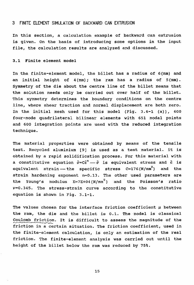
3 FINITE ELEMENT SIMULATION OF BACKWARD CAN EXTRUSION

In this section, a calculation example of backward can extrusion

is given. On the basis of introducing some options in the input

file, the calculation results are analyzed and discussed.

3.1 Finite element model

In the finite-element model, the billet has a radius of 6 (rom) and

an initial height of 4 (rom); the ram has a radius of 5 (rom) •

SYmmetry of the die about the centre line of the billet means that

the solution needs only be carried out over half of the billet.

This symmetry determines the boundary conditions on the centre

line, where shear traction and normal displacement are both zero.

In the initial mesh used for this model (Fig. 3.6-1 (a», 600

four-node quadrilateral bilinear elements with 651 nodal points

and 600 integration points are used with the reduced integration

technique.

The material properties were obtained by means of the tensile

test. Recycled aluminium [9] is used as a test material. it is

obtained by a rapid solidification process. For this material with

a constitutive equation o-=Ccn- 0- is equivalent stress and c is

equivalent strain - the specific stress C=176 (N/rom2) and the

strain hardening exponent n=O. 13 . The other used parameters are

the Young's modulus E=7E+04(N/mm2) and the Poisson's ratio

v=O. 345. The stress-strain curve according to the constitutive

equation is shown in Fig. 3.1-1.

The values chosen for the interface friction coefficient ~ between

the ram, the die and the billet is 0.1. The model is classical

Coulomb friction. It is difficult to assess the magnitude of the~---------",",---,

friction in a certain situation. The friction coefficient, used in

the finite-element calculation, is only an estimation of the real

friction. The finite-element analysis was carried out until the

height of the billet below the ram was reduced by 75%.

15

- -no-=CcC=176 N/mm

2

n=O.13

210

180

.. 150 .E ,E ""- 120

I

z-(/)(f} 90<l)\-.......(/) 60

30

I)1).0 JA- 0.8 1.2 1.6 2.0 2.4

natural strain2.8 3.2 3.6 4.0

Fig. 3.1-1. The stress-strain curve for recycled aluminium

at the temperature of 234 degrees Celsius.

3.2 The selection of elements

ABAQUS contains a library of solid elements for two-dimensional

and three-dimensional application. The two-dimensional elements

allow modelling of plane and axisymmetric problem.

For our problem, only four node axisymmetric elements, CAX4 and

CAX4R, can be used because the finite element mesh of backward can

extrusion must be rezoned several times for protecting the

elements from excessive distortion and other kinds of elements are

not supported for rezoning the finite element mesh by ABAQUS.

The CAX4R and IRS21A, which is a three node contact element and

must be used together with a rigid surface, were selected. The

reason why CAX4R was selected is introduced in the following

Section.

3.2.1 Four node solid isoparametric element

All solid elements used in ABAQUS are isoparametric elements, that

is, coordinate interpolation is the same as displacement.

16

(1) Interpolation

Isoparametric interpolation for the first order isoparametric

element coordinates g, h, shown in Figure 3.2-1. These are also

usually material coordinates, since ABAQUS is a lagrangian code

for most application. They each span the range -1 to +1 in an

element. The interpolation function is as follows:

Fig. 3.2-1. The first order

isoparametric

master element.

(2) Integration

4 r-----------..., 3

11....-------------'2

All of the isoparametric solid elements are integrated

numerically. Two schemes are offered: "full" integration and

reduced integration. Gauss integration is always used because it

is efficient and is especially suited to the polynomial product

interpolations used in these elements.

Reduced integration means that the number of the integration

points less than the "full" scheme is used to integrate the

element's internal forces and stiffness. Superficially this

appears to be a poor approximation, but it has proved to offer

significant advantages. For elements in which the isoparametric

coordinate lines remain orthogonal in the physical space, the

strains are calculated from the interpolation functions with

higher accuracy at these points than where else in the element.

Not only is this important with respect to the values available

for output: it is also significant when the constitutive model is

nonlinear, since the strains passed into the constitutive routines

17

are then a better representation of the actual strains. When

reduced integration is used in the first order elements (the four

node quadrilateral) hourglassing can often make the elements

unusable unless it is controlled. In ABAQUS the artificial

stiffness method of Flanagan and Belytschko (1981) [10] is used to

control the hourglass modes in these elements. The method can be

successful, but it is not a fully robust technique and must

therefore be used with caution.

When discontinuities are expected in the solution (such as

plasticity analysis at large strains), the first order elements

are usually recommended. Reduced integration can be used with such

elements. Fully integrated first order elements should not be used

in cases where "shear locking" [11] can occur, such as when the

elements must exhibit bending behavior.

3.2.2 Interface element and rigid surface

After selecting a four node axisymmetric element CAX4 or CAX4R,

only one kind of interface element, IRS21A, can be used. This is a

three node contact element and is used together with a rigid

surface. It determines whether there is contact between the billet

and the rigid surface or not. When there is contact, the contact

pressure and a possible friction force are calculated. The element

consists of 3 nodes. Two of them are the nodes on a free edge of a

four node element and the third node is a reference node on the

rigid surface.

Two rigid surfaces are defined (see input file in APPENDIX A) and

they are coupled to the groups of interface elements called SECOND

and PUNCH respectively. With the use of the INTERFACE card, two

friction coefficients are defined between the mesh and the

corresponding rigid surface. The friction coefficient has to be

given with a "stiffness in stick". The "stiffness in stick" is an

elastic stiffness which will transmit the shear force across the

element as long as these force are below the friction limit. This

stiffness simulates the fact that there ·should be no relative

18

motion between the surfa,ce until slip occurs. Its

defined by dividing the expected friction limit

acceptable relative displacement before slip

mathematical form of the friction model is described

value can be

force by an

occurs. The

as follows.

A standard Coulomb friction model, with an additional limit on

allowable shear stress is provided in ABAQUS for use with

interface elements.

The kinematic modeling provides a set of three relative

displacements at an integration point associated with the

surfaces: e, the surface over closure; ~, the relative surface3 1

sliding in one direction in the surface; and ~2' the relative

surface sliding in the surface direction orthogonal to that in

which ~ is measured.1

Usually these displacements are only defined as rate. The

kinematic modeling must provide finite increments of these

variables, through some suitable integration of their rates. These

variables will often be in a load system which rotates with the

surfaces. This will give rise to an initial stress term in the

Jacobian matrix, and that term will not be sYmmetric, since the

constitutive term in the Jacobian will not be sYmmetric, the lack

of sYmmetry in the initial stress matrix introduces no additional

penalty.

Let P , Q and Q be surface stresses. We assume that the surfaces3 1 2

are in contact, so that e ~o and P ~O. The Coulomb model is then3 3

defined as follows.

In the normal direction, we assume an elastic behavior:

P =P <e )3 3 3

where the stiffness

E =dP Ide333

19

(3.2-1)

(3.2-2)

where E (£: ) may be allowed to £: =0.3 3 3

In the shear direction, we assume a "strain" rate decomposition

a=1,2

where d1';l is the elastic part of d1'a' and d1'~l represents the

rate of frictional slip.

We assume that this rate decomposition can be integrated over an

increment as

The elastic part of the relative slip,

elastic:

elQ =G. 'Y

a "a'

(3.2-3)

is treated as linear

(3.2-4)

where G is a constant (the "stiffness in stick"), which might be

very large or infinite, and 1'el=~~1'el, summation being taken overa a

all increments since the surface last came into contact.

Slip is governed

(3.2-5)

-sl °Q =min(IlP ,Q )3

where 11 is the friction coefficient, a constant, and QO is a

limiting value of allowable shear stress. This form of the yield

condition is the classical Coulomb model, for IlP <Qo, but has the3

additional shear stress limit, QO. This limit is often useful in

cases involving high contact stress, where the Coulomb

relationship might allow shear stresses that exceed the yield

stress of one of the contacting materials.

20

• sl slIf f::$O at the end of an increment, based on assuml.ng lJ.'1 =lJ.'1 =01 2

during the increment, then no slip has occurred within the

increment. If this is not true, there has been slip. When slip-sloccurs, d'1 is the direction of Q, so that the "flow rule" is

Qd sl d- sl a'1 ='1--a -sl

Q

-slwhere d'1 is the "equivalent slip rate".

(3.2-6)

equation 3.2-3 to 3.2-6 together with the yield condition, define

the model: it is a non associated flow plasticity model.

3.3 Static analysis

In static analysis the solution to a problem is sought assuming

that inertia forces are zero or at most vary slowly throughout the

history.

In ABAQUS two static procedures are provided. One is that the

response to a given load history is sought. Another procedure is

modified Riks algorithm which is usually used for proportional

loading cases, especially when unstable response is possible. The

former procedure was used for our problem.

The analyst has the choice in ABAQUS of solving a static problem

by directly specifying the load incrementation to be followed or

by letting the code choose its own incrementation scheme, based on

user specified tolerances. The former option is useful to the

experienced analyst running a familiar problem. More often,

however the problem is not familiar and the option of letting

ABAQUS choose appropriate load step is the most valuable. So the

latter one was chosen.

On the data card following the *STATIC option, the user specifies

a suggested "time" increment and a total "time" for the static

21

solution. For example, for the problem of backward can extrusion.

*STATIC,PTOL=50

0.1,1

where 0.1 is a suggested "time" increment and 1 is a total

"time". "time" here is usually understood as a normalized time and

is used for convenience in referring load parameters to *

AMPLITUDE references. ABAQUS begins the solution of a static step

with the user specified suggested increment of time. This time

increment will be increased or decreased as described below.

Given an increment size, ABAQUS monitors the maximum force and

moment residuals. If Rell denotes the maximum residual at the i th

iteration, the solution

Otherwise at iteration

predicted, i.e.

is considered converged when Ro):sPTOL.

i, the convergence at iteration n is

n=i+In (PTOL/Re II ) / In (Re II /RO-ll ) (the derivation is omitted).

If n exceeds m, the maximum number of iterations permitted in an

increment, the following occurs:

(a). if n>m, the increment is considered too large, and is cut

to 1/4 of its size. The solution is then started over again from

the end of the previous increment.

(b). if n<m, the iteration is continued.

(c). if, in two successive increments, convergence is achieved

in less than m/2 iterations, the increment size is increased by

25% for the next increment.

The maximum increment in a static analysis step and the maximum

number of iterations in a increment are given by user. For the

problem of backward can extrusion, they were specified as follows;

*STEP,INT=200,CYCLE=10,SUBMAX,AMP=RAMP,NLGEOM

where the "INT" is used to specify the maximum number of

22

increments according to the solved problem. the "CYCLE" is used

to specify the maximum number of iterations. The default value is

6 and should be sufficient in most smoothly nonlinear cases. This

value should be changed to 10-15 for problems with discontinuous

behavior, such as problems involving sudden changes in stiffness

associated with contact (cases' with interface elements). In such

cases the SUBMAX parameters is also usually used to suppress

subdivision except when convergence is not achieved in the maximum

number of iterations allowed, the "NLGEOM" indicates geometric

nonlinearity should be accounted for during the step and the

"AMP=RAMP" indicates the displacement of the ram varies linearly

over the step with the time variation.

3.4 Constitutive relationship

various elastic response model are provided in ABAQUS. The

simplest one of these is linear elasticity:

- el -el<T=D : c

where Del is a matrix that does not depend on the deformation. In

ABAQUS this elasticity model is intended to be used for small

strain problems or to model the elasticity in an elastic-plastic

model in which the elastic strains are always small. This type of

behavior is defined in the *ELASTIC material options (see APPENDIX

A) •

Incremental plasticity theory is based on a few fundamental

postulates, which means that all of the elastic-plastic response

models provided in ABAQUS have the same general form. The metal

plasticity model either as a rate dependent or as rate independent

model has a particularly simple form.

For simplicity of notation all quantities not explicit associated

with a time point are assumed to be evaluated at the end of the

increment.

23

The Van Mises yield function with associated flow means that there

is no volumetric plastic strain, and since the elastic bulk

modulus is quite large, the volume change will be small, so that

we can define the volume strain as

e: =trace(E) ,vol

and hence the deviatoric strain is

- 1e=e:- - e: I3 vol

The strain rate decomposition is:

- -el -pIde:=de: +de:

Using standard deformation of co-rotational measures, this can be

written in integrate form as

- -el -pIe:=e: +e: . (3.4-1)

The elasticity is linear and isotropic, and may therefore be

written in terms of two temperature dependent material parameters.

For the purpose of this development it is most appropriate to

choose these parameters as the bulk modulus, K, and shear modulus,

G. These are readily computed from the user's input of Young's

modulus, E, and Poisson's ratio, v, as

EK= 3(1-2v) and G= -:-'i"":E:-:---.-­2(1+v)

The elasticity may then be written as

P=-Ke:vol'

where

1 -P=-""'3 trace (0-)

24

(3.4-2)

is the equivalent pressure stress.

Deviatoric:

strain rate. Plasticity

uniaxial stress-plastic

the material is rate

S=2Geel ,

where S is the deviatoric stress:

S=u+pI

The flow rule is

PI -pIde =de n,

where

3 Sn=T q

and dePI is the equivalent plastic

requires that the material satisfies a

strain-strain rate relationship. If

independent this is the yield condition:

(3.4-3)

(3.4-4)

(3.4-5)

where uO(eP1 ,8) is the yield stress, and is defined by the user as

a function of equivalent plastic strain (eP1) and temperature (8).

In our problem, Uo only is the function of equivalent plastic

strain.

The material behavior is defined as a linear elastic behavior in

combination with a nonlinear plastic behavior. But the

stress-strain curve is defined in piece wise linear segments in

the *PLASTIC option up to a total plastic strain level of 3.798.

25

The yield stress remains constant for plastic strains exceeding

the last value given (see Appendix A).

3.5 Mesh rezoning

ABAQUS [12] is a Lagrangian program, in the sense that the mesh is

attached to the material and thus deforms with the material. When

the strains become large in geometrically nonlinear analysis (with

the NLGEOM parameter set on the procedure card), the elements may

become so severely distorted that they no longer provide a good

discretization of the problem. When this occurs it is necessary to

flrezon": to map the solution onto a new mesh which is better

designed to continue the analysis.

The first requirement for rezoning is some indication that the

mesh is becoming distorted in regions where this may cause the

solution to be inaccurate. One possible criterion for rezoning

would be extreme element distortion in areas of high strain

gradients. Once the user has decided that the mesh needs rezoning

he must generate a new mesh that is more suitable to the current

state of the problem.

The simulation is continued by interpolating the solution onto the

new mesh from the restart file generated with the old mesh. This

is done in the *INITIAL CONDITIONS option, using the parameter

TYPE=OLD MESH, and specifying the step number and increment number

at which solution should be read from the restart file. The

interpolation technique used in this operation is to obtain the

solution variables at the nodes of the old mesh: this is done by

extrapolating all values from the integration points to the nodes

of each element, and averaging those values over all elements

abutting each node. Then the location of each integration point in

the new mesh is obtained with respect to the old mesh. The

variables are then interpolation from the nodes of the element to

that location. All necessary variables are interpolated

automatically in this way, so that the solution can proceed on the

new mesh.

26

Whenever the solution is rezoned it can be expected that there

will be some discontinuity in the solution because of the change

in the mesh. If the discontinuity is significant it is an

indication that the meshes are too coarse, or that the rezoning

should have been done at an earlier stage before too much

distortion occurred. Provide that the meshes are sUfficiently fine

for the problem and that the rezoning is done before the elements

too distorted, the technique works well.

The mesh was rezoned totally 59 times and the ram was moved down

0.05 (mm) each time for protecting the elements from excessive

distortion which makes the calculation not convergent and further

analysis impossible because the backward can extrusion problem is

a large deformation problem.

3.6 Results and discussion

3.6.1 Deformed mesh

Fig 3.6-1 shows the rezoned meshes and deformed meshes at each 25%

deformation up to 75% besides the initial mesh and the first

deformed mesh. In order to continue a large deformation analysis

with sufficient accuracy it will be necessary to regenerate a new

mesh. But in ABAQUS there is not this kind of function by means of

which the mesh can be rezoned automatically. Therefore, a mesh has

to be rezoned by rewriting the input file. This takes a lot of

time. Another defect which has been found is that the element on

the sharp corner will cut across the sharp corner of the ram.

After rezoning the mesh, some material will be lost, because there

is just a node of the rezoned mesh on the sharp corner. Therefore,

the height of the can from finite element simulation is less than

that from practical product. If the eight node elements are used

to generate the mesh, the defect can be overcome and the accuracy

is better than that of four node elements, but the mesh of eight

node element can not be rezoned in ABAQUS.

27

(a) Initial mesh and the first deformed mesh.

(b) Rezoned mesh and 25% deformed mesh.( ~~ c; c {" /0-tc/£,Vl,..c&:lu{.f .,< OtAAC It_

(c) Rezoned mesh and 50% deformed mesh.

28

(d) Rezoned mesh and 75% deformed mesh.

Fig. 3.6-1. Rezoned mesh and deformed mesh (The deformation is

defined as the percentage of displacement at any

instantaneousness and total displacement of the ram).

3.6.2 Equivalent stress and strain

Fig. 3.6-2 shows the contour plots of equivalent stress and strain

at each 25% deformation up to 75%. The contour plots on the first

deformed mesh also are shown.

In the contour plots of equivalent stress, some facts can be paid

attention to. The highest stress gradient is concentrated around

the sharp corner of the ram. As the ram is moved down, there

exists always stress in the elements which are moving up. This is

not normal. The reason is because after rezoning the mesh each

time, the stress in the old mesh will be interpolated to the new

mesh (see section 3.5). The contour plots of equivalent stress

show this fact clearly.

29

(a) Initial deformation.

Equivalent

stress

1=6. 24E+07

2=6. 86E+07

3=7. 48E+07

4=8.10E+07

5=8. 73E+07

6=9. 35E+07

(b) 25% deformation.

I,

Equivalent

stress

1=7. 39E+07

2=9. llE+07

3=1.08E+08

4=1.25E+08

5=1. 43E+08

6=1.60E+08

Equivalent

stress

(e) 50% deformation.

30

1=9. 15E+07

2=1.07E+08

3=1. 23E+08

4=1.38E+08

5=1.54E+08

6=1.70E+08

Equivalent

stress

1=5.08E+07

2=7. 56E+07

3=1.00E+08

4=1.25E+08

5=1.50E+08

6=1.75E+08

(d) 75% deformation.

Fig. 3.6-2. The contour plots of equivalent stress (N/m2) (left)

and equivalent strain (right).

From the contour plots of equivalent strain it can also be

observed that the highest strain gradient and the biggest

equivalent strain are also concentrated around the sharp corner,

but with the movement of the ram they move to lower right hand

corner gradually.

3.6.3 Extrusion force

Fig. 3.6-3 shows the finite element solution and experimental

solution of the extrusion force. From these two curves it can be

seen that a good agreement is obtained between the finite element

solution and the experimental solution when the deformation is

less than or equal to 30%. But with the increase of the

deformation, the difference between the finite element solution

and the experimental solution increases gradually. It is due to

the algorithm of ABAQUS. First, when the mesh is rezoned each

31

time, the stress in the old mesh is always interpolated to the new

mesh. Therefore, the upper stress of extruded can can not be

released. Secondly, because the upward elements always touch the

rigid surface and there exists the normal stress in the radial

direction of the ram in these elements, there exists friction

force between the rigid surface and elements (see section 3.2.2).

As a matter of fact in practical extrusion of a can the friction

force does not exist after the extruded material moves up to a

certain height. The extra friction force was exerted to the

extruded material as a force constraint. Therefore, the extrusion

force increases rapidly with the increase of the friction force or

the rise of the material.

iii I

0.6 1.2 1.8 2.4Displacment of the ram (mm)

finite element solutionexperimental solution

I

3.0

ao!iaaa

............ 0Z 90 6.~'-"

Q}

u~

0 604-

C0en::J~

-+J

XW

120

Fig. 3.6-3. Displacement-extrusion force curves.

The selection of friction coefficients has an important influence

on the extrusion force and convergence of solution. If a higher

value of the friction coefficient is selected, the extrusion force

will be much higher than the experimental one. If the friction

coefficient is very small, the excessive distortion of some local

32

elements will occur and result in poor convergence.

After the mesh is rezoned each time, normally the discontinuity of

the extrusion force will occur (not shown in Fig. 3.6-3). Because

in a step the ram was only moved down O.05(mm) and then the mesh

was rezoned again, the discontinuity is very small. The deviation

is within 6%. If the displacement of the ram is increased in a

step the force discontinuity will also increase. Therefore, in

each step the selected displacement of the ram should not be too

large to maintain the necessary accuracy.

3.6.4 Triaxiality

Another important application about the finite element simulation

of metal forming processes is the determination of ductile failure

during the forming processes, such as backward can extrusion.

Because the triaxiality and equivalent strain distribution in

material inner can be observed through finite element analysis, it

is possible to determine the occurrence of ductile failure. r

However, the corresponding ductile failure curve for this kind of

material must be determined first. Fig. 3.6-4 shows the contour

plot of triaxiality when the deformation of the mesh is 75%.

Fig. 3.6-4. The contour plot

of triaxiality.

33

Trlaxlallty

1=-18.81

2=-15.77

3=-12.74

4=-9.70

5=-6.67

6=-3.63

4 FINITE ELEMENT SIMULATION OF THE TENSILE TEST

liCll (llel rJ;J

This section deals with the finite element simulation of a tensile

test in ABAQUS. The purpose is to verify the correctness of the

Bridgman model that describes the stress state in an unnotched

specimens. It is generally not possible that the necking of the

unnotched specimen is simulated by a finite element method. But

through taking measures, the finite element simulation was made

approximately. Some main options in this input file have been

mentioned in section 3, that will not be repeated in this section.

4.1 Finite element model

In the finite element model, the specimen has a radius of 10{mm)

and an initial length of 110{mm). It is due to the sYmmetry of the

specimen that the solution needs only be carried out over a

quarter of the specimen. This symmetry determines the boundary~._~

conditions on both the axis and the centre line, where shear

traction and normal displacement are both zero. The loading was

applied by a end displacement. In the initial mesh used for this

model (Fig. 4.1-1), 480 four node quadrilateral bilinear elements

with 533 nodal points and 480 integration points were used with

the reduced integration technique.

For simulating the necking of the specimen, the two ends of the

initial mesh are of slightly different radii. One end on which the

centre line is contained has a radius of 9.9{mm). Hence, necking

can occur, otherwise the finite element model can not simulate the

necking of cylindrical bars.

(11,'Q,

-- I<lf~

Fig. 4.1-1. The initial mesh of tensile specimen.

34

About the material properties, these were taken for aluminium: the

Poisson's ratio v=O.345 and the Young's modulus E=7.06E+04(N/mm2).

The used constitutive equation is u=Ccn• The specific stress C is

176(N/mm2). The strain hardening exponent is taken from n=O.OO to

0.28 at intervals of 0.04. Therefore, eight calculations were

carried out with different strain hardening exponent. The input

file is shown in APPENDIX A.

4.2 Bridgman model

Fig. 4.2-1. Diagram

of Bridgman model.

radius

(4.2-2)

smallest

(4.2-1)

radius of the

is the initial

2 2

O"m/U=1/3+ln(1+ a2~~ )

E:ave=2ln(a fa)o

- 2O"=F/ (lla ) ,

cross section, ao

of the specimen, r is the coordinate position in the smallest

cross section in the radial direction, and R is the radius of

profile arc. These parameters are shown in Fig. 4.2-1.

where a is the

E:ave=2ln(a fa) ,o

O"m=(1/3)U.

During necking according to the Bridgman

model (1952) [8] under the assumption of

homogeneous deformation in the area of

the smallest cross section the equivalent

strain and triaxiality in the smallest

cross section are

In a tensile test with a cylindrical test

specimen, before necking it holds

Because cracking starts in the centre of the tensile test

35

specimen, our interest is concentrated on it. Equation 4.2-2 with

r=O gives

umjU=lj3+ln(1+aj2R).

4.3 Results and discussion

(4.2-3)

4.3.1 The finite element meshes of the necking process

Fig. 4.3-1 shows the finite element meshes of the necking process

with which the calculation was made with a strain hardening

exponent n=O.20. The necking processes of other two finite element

meshes with n=O.OO and n=O.28 are shown in APPENDIX B.

Ca) The end displacement is 12(mm).

(b) The end displacement is 13(mm).

(c) The end displacement is 14(mm).

(d) the end displacement is 15(mm).

36

(e) The end displacement is 16(mm).

- ....

(f) The end displacement is 17(mm).

(g) The end displacement is 18(mm).

Fig. 4.3-1. The finite element meshes

of the necking process (n=O.20).

4.3.2 Equivalent strain

The distribution and change process of the equivalent strain

during necking are shown in Fig. 4.)-2. From that you can derive

that the maximum equivalent strain occurs at the sYmmetric centre

of the necked bar. It means that the ductile failure may initiate

at the centre part. Previous research work [14] has proved this

fact. Therefore, the main interest is aimed at this part. But

ductile failure does not certainly occur in the part where the

highest equivalent strain value takes place. It must be considered

in combination with the triaxiality [23].

37

I, 2 J 4 5 6

I 2 J 4 5 Ii, 2 J 4 5Ii,

~ 2 J 4 5,~, 2 J 4 5

(a) The end displacement is 12(mm}.

L- illli(l(b) The end displacement is 13(mm}.

lnillJ' 2 J ~

, 2 J 4 S, 2 J 4 S

, 2 J 4 5 :, 2 J 4 5 6

---------------------------

(c) The end displacement is 14(mm}.

111(}' JI 2 J ~ SI 2 4 6

~ ~ ~ ~ ; :1..- _

(d) The end displacement is 15(mm}.

JJmzJ'

II \ J 4 53 4 5 6

I ~ J 4 5 6I 2 J 4 5 6

-----------------------------

(e) The end displacement is 16(mm}.

38

~~2I 2 • 5J • 5 6I J • 5

~ i i ~ ~ f6'------------------------------

(f) The end displacement is 17(mm).

II

(g) The end displacement is 18(mm).

Fig. 4.3-2. The contour plots of equivalent strain.

4.3.3 Triaxiality

Fig. 4.3-3 shows the contour plots of triaxiality. Before necking

the triaxiality is 1/3 in the whole test specimen. During necking

the maximum triaxiality is located at the centre part. Therefore,

only the centre part needs to be considered to obtain the

triaxiality for various application. Because it is not possible

that the triaxiality and equivalent strain are taken at the

symmetric centre point, the element which is close to centre point

is used to get above values approximately.

(a) The end displacement is 12(mm).

39

__~·a(b) The end displacement is 13(mm) .

..Ii__A---:--

(c) The end displacement is 14(mm).

(d) The end displacement is 15(mm).

(e) The end displacement is 16(mm).

(f) The end displacement is 17(mm).

40

6

(g) The end displacement is 18{mm).

Fig. 4.3-3. The contour plots of triaxiality.

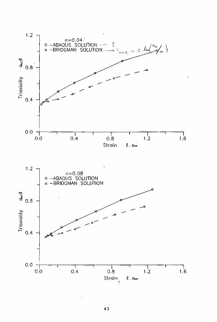
4.3.4 The curves of the triaxiality versus the strain

The triaxiality curves versus both equivalent strain c and mean

strain ea~ in the smallest cross section (see equation 4.2-1) are

shown in Fig. 4.3-4. The curves of the triaxiality versus the

equivalent strain were obtained from the finite element solution.

The curves of the triaxiality versus the mean strain were obtained

from the Bridgman model in which the radius of the smallest cross

section and the radius of profile arc of necking also were taken

from the finite element mesh. The radii R of profile arc were

calculated in a radius fitting program with a least-squares

procedure. During the calculation it was found that the results of

Bridgman model have a better agreement with the finite element

results when three nodes which are the most close to the smallest

cross section are used to calculate the radius of profile arc. The

more the fitting points used, the larger the radius of profile arc

and the smaller the triaxiality from the Bridgman model and the

bigger the difference between the finite element solution and

Bridgman solution. Therefore, the radius of profile arc was

calculated out of the position of three central nodes.

From these curves some interesting phenomena are observed. For any

strain hardening exponent n the triaxiality difference between the

finite element solution and Bridgman solution increases with the

increase of the strain and decreases with the increase of the

strain hardening exponent n. The former can be understood in the

following way. with the increase of the end displacement of the

specimen the nodes are far from the smallest cross section

41

gradually. Therefore, the difference increases (see the element

meshes in Fig. 4.3-1). This problem can be solved easily by

rezoning the element mesh before the elements in the smallest

cross section suffer excessive deformation. For the second it

holds: the Bridgman model was obtained under the condition that

the elements in the smallest cross section are deformed uniformly

[15]; the nonuniform element deformation in the smallest cross

section will influence the accuracy of the Bridgman model. More

uniform element deformation in the smallest cross section can be

observed in Fig. 4.3-1 and Fig. B.2-1 and the nonuniform element

deformation can be seen in Fig. B.1-1. Therefore, the triaxiality

difference between finite element solution and Bridgman model

solution will decrease with the increase of strain hardening

exponent n. Fig. 4.3-5 shows the triaxiality difference when the

equivalent strain c=l. O. It is due to the same reason that the

difference between the equivalent strain in the central element

and the average strain in the smallest cross section also

decreases with the increase of the strain hardening exponent n

during necking (see Fig. 4.3-6).

1.2n=O.OO

o - J,BA.QUS SOLUTION6. - BRIDGMAN SOLUTION

Ib"~ 0.8 ,4---->- ~.....

,.../

a ,.../

x ~a ../"

'C .,.A~

0.4 ~

0.0

0.0 0.4 0.8Strain e. to••

1.2I

1.6

42

1.2

10"-~ 0.8-

oxo

'Cl- OA

n=0.04 .o -ABAQUS SOLUTION --'\ ~6. -BRIDGMAN SOLUTION .---'", 't. :::- Z.

O-~ .

--I!..­..-

-

0.00.0 004 0.8 1.2

Strain l. EAve

1.6

1.2n=0.08

o -ABAQUS SOLUTION6. -BRIDGMAN SOLUTION

'0"-t! 0.8

,At.

>. --...... -r0 --X I!..--0 ..-

'C ~l- OA -

0.00.0 OA 0.8 1.2

Strain l. EAve

1.6

43

1.2

'0......

~ 0.8

oxo

'C..- 0.4

n=0.12o -ABAQUS SOLUTIONa -BRIDGMAN SOLUTION

0.00.0 0.4 0.8

Strain1.2

I1.6

1.2 -,

'0......

~ 0.8

>-.....oxo

·C..- 0.4

n=0.16o -ABAQUS SOLUTIONa -BRIDGMAN SOLUTION

0.00.0 0.4 0.8

Strain

44

l. £0..

1.2 1.6

1.2n=0.20

o -ABAQUS SOLUTION6. -BRIDGMAN SOLUTION

lb......

~ 0.8

axa'CJ-

0.4

0.00.0 ..

1.2

0.4

---~

0.8Strain

- -

1.2 1.6

n=0.24o -ABAQUS SOLUTIONu - BRIDGMAN SOLUTION

'b-...~ 0.8

axa'CJ- O.4

0.00.0 0.4

11.-­-11.­-

0.8Strain

45

g . lAve

-

1.2

-

1.6

1.2 -,n=0.28

o -ABAQUS SOLUTION6. - BRIDGMAN SOLUTION

Ib......

~ 0.8

axa

'Cl- OA

0.00.0 004 0.8

Strain ~ . E:o.e

1.2 1.6

Fig. 4.3-4. The curves of the triaxiality versus the strain.

0.30

£=1.00.24

>--+oJ

ax 0.18a--0Q) 0.12ucQ)~

Q)'+-

0.06'+-

0

0.300.00

0.00 0.06 O. 12 0.18 0.24Strain hardening exponent

Fig. 4.3-5. The difference of triaxiality between the finite

element solution and the Bridgman model solution.

46

2.00 2.0n=O.OO n=0.04. j. )( )(

<31.50 / 1.5 /

c: / c: /0 a'-

/''-- ..... /III 1.00 III 1.0

/ Lc: / c:0 0Q) Q) ~~

0.50~

0.5

0.00 0.00.0 0.5 1.0 1.5 2.0 0.0 0.5 1.0 1.5 2.0

Equivalent strain ~ Equivalent strain ~

2.0 2.0

• n=0.08 n=0.12..; x j *

1.5 / 1.5 /c:

/c: /0 0.... '-.....

~ -III 1.0 III 1.0c: b c:0 aQ) Q)

::E 0.5 ~0.5

0.0 0.00.0 0.5 1.0 1.5 2.0 0.0 0.5 1.0 1.5 2.0

Equivalent strain ~ Equivalent strain ~

2.0 2.0n=0.16 n=0.20

I.. x

" J~ /1.5 / 1.5c: /

c:0 a'- '- ,1.....

/-III 1.0III 1.0

c: c: ,f-a 0Q) Q)

~0.5

:!E0.5

/0.0 0.0 /

0.0 0.5 1.0 1.5 2.0 0.0 0.5 1.0 1.5 2.0

Equivalent strain ~ Equivalent strain £.

47

2.0 2.0n=0.24 n=0.28

: ..)( > )(t.S ~

1.5 - / 1.5 /c c0 0'- L........ ...... #III 1.0 III 1.0c c #0 0Q.I Q.I

~0.5 - ~

0.5

~r0.0 0.0 I I0.0 0.5 1.0 1.5 2.0 0.0 0.5 1.0 1.5 2.0

Equivalent strain ~ Equivalent strain l

Fig. 4.3-6. The curves of the equivalent strain in the central

element versus the mean strain in the smallest cross

section.

The fact that the difference of triaxiality between the ABAQUS

solution and Bridgman model solution decreases with the increase

of the strain hardening exponent n indicates that the problem can

probably be solved by finding an appropriate correction parameter

for this behavior. But the correctness of the Bridgman model

solution on which some parameters are taken on the deformed finite

element mesh must be verified by obtaining these parameters on a

corresponding tensile test specimen.

4.3.5 The comparison of the ABAQUS solution

and the MARC solution of triaxiality

Fig. 4.3-7 shows the curves of the triaxiality versus the

equivalent strain which were got in ABAQUS and in MARC [14 ]

respectively. These curves indicate a rough agreement. The

difference between the ABAQUS solution and MARC solution can not

be analyzed because the different parameters such as the specific

stress C, the Young's modulus E and Poisson's ratio v were used.

The parameters used in ABAQUS are taken from aluminium and the

parameters used in MARC are obtained from Armco (n=0.26) and Steel

1022 (n=0.19).

48

1.2

o -ABAQUS SOLUTION (n=0.20)a -MARC SOLUTION (n=0.19)

'b"~ 0.8

oxo

'CI-

0.4

0.00.0 0.4 0.8 1.2

Equivalent strain ~

1.6

1.2

Ib

".j 0.8

ox\]

~

l- OA

o -ABAQUS SOLUTiON (n=0.24)a -MARC SOLUTION (n~0.26) .t:. -ABAQUS SOLUTION (n=0.28)

o.0 -+------.------.---~--.......__--.___--,_--r_-____,

0.0 0.4 0.8 1.2Equivalent strain ~

1.6

Fig. 4.3-7. The comparison of the ABAQUS solution

and the MARC solution.

49

5 CONCLUSIONS

According to the above-mentioned results and analyses, the

following conclusions can be obtained.

The finite element simulation of metal forming processes can be

carried out completely in ABAQUS. But some defects of ABAQUS have

been found in solving some metal forming problem such as the

backward can extrusion problem. One defect is that the mesh can

not be rezoned automatically and the mesh can only be rezoned by

rewriting the input file. It takes a lot of time. Another defect

is that the eight node element is not supported for rezoning by

ABAQUS. If four node elements are used, some material will be lost

after rezoning the mesh. This can be solved by developing an

automatic rezoning technique for ABAQUS and making the element

mesh very fine around the sharp corner.

After rezoning the mesh, a discontinuity in the reaction force

occurs; the less the displacement of the ram for each rezoning of

the mesh, the smaller the discontinuity. In the backward can

extrusion problem the force discontinuity is less than 6%.

The friction coefficient must properly be selected for the

backward can extrusion problem. Otherwise, poor convergence will

occur. The friction force between the ram, the die and the billet

has a significant influence on the extrusion force. The question

is how the influence of extra friction force action on the side

walls can be eliminated? Further research work needs to be done.

The necking process in the tensile test can be simulated by the

finite element method, under the condition that radius tolerance

can be given. If not, it is not possible to simulate the necking

of an unnotched cylindrical specimen.

If the triaxiality is calculated with the Bridgman model in which

some parameters are 'taken from the deformed finite element mesh,

it will indicate a better agreement with the finite element

50

solution when three nodes which are the most close to the smallest

cross section are used to calculate the radius of profile arc.

This result also indicates that when the triaxiality of a

cylindrical specimen in a tensile test is calculated with the

Bridgman model, higher accuracy will be attained if the measured

points for calculating the radius of profile arc of tensile test

specimen are close to the smallest cross section.

The difference of triaxiality between the ABAQUS solution and the

Bridgman model solution increases with the increase of the strain

for any strain hardening exponent n. This can be solved by using a

mesh rezoning technique which keeps the elements in the smallest

cross section not excessive elongation in the axis direction.

The difference of triaxiality between the ABAQUS solution and the

Bridgman model solution decreases with the increase of the strain

hardening exponent n. It indicates sUfficiently that the Bridgman

model has a higher accuracy if the strain in the smallest cross

section is more uniform, because the higher the strain hardening

exponent n, the more uniform the strain in the smallest cross

section. If an additional parameter, depending on the strain

hardening exponent and the equivalent strain, is put in the

Bridgman model, the calculation accuracy of the Bridgman model

will be improved. Besides that the calculation method with which

the radius is computed by taking the node coordinates from the

deformed mesh must be verified by experiment.

The ABAQUS solution of triaxiality has a better agreement with the

MARC solution on the tendency of the triaxiality change. This

indicates that it is also valid that this kind of problem is

solved in ABAQUS.

51

ACKNOWLEDGEMENT

By means of this thesis, I would be much obliged to those people

in the Group of Production Technology and Automation, who gave me

so much help during my study and research so that I could finish

all courses and this thesis.

Especially, first I would like to express my gratitude to Prof.

ire J.A.G. Kals and dr. ire J.H. Dautzenberg who gave me the

opportunity to carry out my Second Phase study at Eindhoven

University of Technology.

Secondly, I acknowledge my coach, dr. ir. J. H. Dautzenberg, my

supervisor, Prof. ir J.A.G. Kals, ir F.A.C.M. Habraken and dr. ire

W.H. Sillekens for their guidance and help during my project and

writing the thesis.

Finally, I thank my wife and my parents for their unreserved

support for my overseas study.

52

REFERENCES

1. T.J. Chung, "continuum Mechanics", PRENTICE HALL, 1989.

2. R.M. McMeeking and J.R. Rice,"Finite Element Formulations for

Problems of Large Elastic-Plastic Deformation", Int. J. Solids

Structures, vol. 11, pp. 601-616, 1975.

3. P. Hartley, C.E.N. Sturgess and G.W. Rowe,"A Finite Element

Analysis of Extrusion-forging", Proc. 6th North American Metal

Working Research Conf., pp. 212-219, 1978.

4. P. Hartley, C. E. N• Sturgess and G. W. Rowe, "Prediction of

Deformation and Homogeneity in Rim-disc Forging", Journal of

Mechanical Working Technology, 4, pp. 145-154, 1980.

5. A.A.M. Hussin, P. Hartley, G.W.N. Sturgess and G.W. Rowe,

"Elastic-Plastic Finite-element Modelling of a cold-extrusion

Process using a Microcomputer-based System", Journal of

Mechanical Working Technology, 16, pp. 7-19, 1988.

6. G.J.M. Gelten and A.W.A. Konter,"Application of Mesh-rezoning

in the Updated Langrangian Method to Metal Forming Analysis",

Numerical Method of Industrial Forming Processes, Proc. of the

Inter. conf., pp. 511-521, 1982.

7. J.S. Park and S.M. Hwang,"Automatic Remeshing in Finite

Element Mesh Simulation of Metal Forming Processes by Guide

Grid Method", Journal of Materials processing Technology, 27,

pp. 73-89, 1991.

8. P. W. Bridgman, "Studies in Large Plastic Flow and Fracture",

McGRAW-HILL Book Company, 1952.

9. W.H. Sillekens, J.H. Dautzenberg and J.A.G. Kals,"Formability

of Recycled Aluminium-Advantages of a Rapid Solidification

Process", Annals of the CIRP, Vol. 39/1, pp. 287-290, 1990.

10. D.P. Flanagan and T. Belytschko,"A Uniform strain Hexahedron

and Quadrilateral with orthogonal Hourglass Control", Inter.

Journal for Numerical Method in Engineering", Vol. 17, pp.

679-706, 1981.

11. J.C. Nagtegaal, D.M. Parks and J.R. Rice,"On Numerically

Accurate Finite Element Solutions in the Fully Plastic Range",

Computer Methods in Applied Mechanics and Engineering, 4, pp.

153-177, 1974.

53

12. Hibbitt, Karlsson and Sorensen, Inc., "ABAQUS User's Manual",

Version 4.7, 1988.

13. Hibbitt, Karlsson and Sorensen, Inc., "ABAQUS Theory Manual",

Version 4.8, 1989.

14. P.J. Bolt,"Prediction of Ductile Failure", Ph.D. Thesis of

Eindhoven university of Technology, 1989.

15. T.G.S. Bollen,"Ductile Failure", M.Sc. Thesis of Eindhoven

University of Technology, 1990.

16. R. Hill, "The Mathematical Theory of Plasticity", OXFORD PRESS,

1950.

17. A. Needleman, "A Numerical

cylindrical Bars", J. Mech.

Study

Phys.

of Necking in

Solids, Vol.

circular

20, pp.

111-127, 1972.

18. A. Needleman and V. Tvergaard,"An Analysis of Ductile Rupture

in Notched Bars", J. Mech. Phys. Solids, Vol. 32, pp. 461-490,

1984.

19. H.D. Hibbitt, P.V. Marcal and J.R. Rice,"A Finite Element

Formulation for Problems of Large strain and large

Displacement", Int.J. Solids Structure, Vol. 6, pp. 1069-1086,

1970.

20. Ranbir S. Sandhu and Kamar J. Singh, "Reduced Integration for

Improved Accuracy of Finite Element Approximations", Computer

Methods in Applied Mechanics and Engineering, 14, pp. 23-27,

1978.

21. N. Bicanic and E. Hinton, "Spurious Modes in Two-Dimensional

Isoparametric Elements", Int. J. for Numerical Methods in

Engineering, Vol. 14, pp. 1545-1557, 1979.

22. Y.Q. Xie and F.B. He,"Finite Element Method in Elasticity and

Plasticity", China Machinery Press (in Chinese), 1982.

23. W.H.Sillekens,"Backward Can Extrusion and Materials Behavior",

Ph.D. Thesis of Eindhoven University of Technology, 1992.

54

APPENDIX A INPUT FILES

A.1 The input file of the backward can extrusion problem

In solving the backward can extrusion problem, the finite element

mesh was rezoned several times. For each rezoning an input file

has to be written. Because there is only little difference between

these input files, only one example is given.

I*HEADING

!BACKWARD CAN EXTRUSION PROBLEM

*RESTART,WRITE,FREQ=20

***********************************************************

*NODE

1,0,0

30,S.8E-03,0

'SOl,0,1.0SE-03

S30,S.8E-03,1.0SE-03

S31,6E-03,1.0SE-03

131,6E-03,2E-04

31,S.98SE-03,1.SE-OS

.8888, 6E-03, 0

9999,0,7.0SE-03

*NODE,NSET=TOP1

4826,S.0000E-03,9.8392E-03

4827,S.2007E-03,9.8S02E-03

4828,S.3997E-03,9.8682E-03

4829,S.S993E-03,9.8784E-03

4830,S.7997E-03,9.88S4E-03

4831,6.0000E-03,9.8868E-03

*NGEN,NSET=APPEN

131,S31,100

*NGEN,NSET=BOT

1,30

*NGEN,NSET=TOP

SOl,S30

*NFILL

SS

BOT,TOP,5,100

*NSET,NSET=MIDDLE,GEN

526,531,1

*NFILL

MIDDLE,TOP1,43,100

*NSET, NSET=SIDE1, GEN

526,4826,100

*NSET,NSET=SIDE2,GEN

531,4831,100

*NSET,NSET=ALL

9999,APPEN,TOP1,SIDE1,SIDE2

*NSET,NSET=AXIS,GEN

1,501,100

***********************************************************

*ELEMENT,TYPE=CAX4R,ELSET=METAL

1,1,2,102,101

626,526,527,627,626

*ELGEN,ELSET=METAL

1,30,1,1,5,100,100

626,5,1,1,43,100,100

*ELSET.ELSET=LITTL,GEN

1,401,100

*ELEMENT,TYPE=IRS21A

7701,4831,4731,8888

6601,31,30,8888

9901,501,502,9999

9926,526,626,9999

*ELGEN,ELSET=SECOND

7701,48,-100,1

6601,30,-1,1

*ELGEN,ELSET=PUNCH

9901,25,1,1

9926,43,100,1

***********************************************************

*RIGID SURFACE,ELSET=SECOND,TYPE=SEGMENTS,SMOOTH=0.00005

START,-O.OOl,O

LINE,O.006,O

56

LINE,O.006,O

*INTERFACE,ELSET=SECOND

*FRICTION

O.1,lE+11

*RIGID SURFACE,ELSET=PUNCH,TYPE=SEGMENTS,SMOOTH=O.00005

START,O.005,1.005E-02

LINE,O.005,1.05E-03

LINE,-O.OOl,1.05E-03

*INTERFACE,ELSET=PUNCH

*FRICTION

O.1,lE+11

***********************************************************

*SOLID SECTION,ELSET=METAL,MATERIAL=EL

*MATERIAL,NAME=EL

*ELASTIC

70E+09,O.345

*PLASTIC

7.1957E+07,O.OOO

1.4287E+08,O.199

1. 5629E+08, 0.399

1.6473E+08,O.599

1.7100E+08,O.799

1.7602E+08,O.999

1.8024E+08,1.198

1. 8389E+08, 1. 398

1. 8710E+08, 1. 598

1.9000E+08,1.798

1.9261E+08,1.998

1.9501E+08,2.198

1.9723E+08,2.398

1.9929E+08,2.598

2.0122E+08,2.798

2.0303E+08,2.998

2.0474E+08,3.198

2.0636E+08,3.398

2.0790E+08,3.598

2.0936E+08,3.798

57

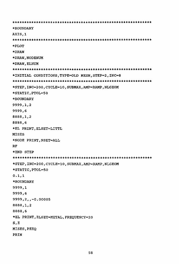
************************************************************BOUNDARY

AXIS, 1

************************************************************PLOT

*DRAW

*DRAW,NODENUM

*DRAW,ELNUM

************************************************************INITIAL CONDITIONS,TYPE=OLD MESH,STEP=2,INC=8

************************************************************STEP,INC=200,CYCLE=10,SUBMAX,AMP=RAMP,NLGEOM

*STATIC,PTOL=50

*BOUNDARY

9999,1,2

9999,6

8888,1,2

8888,6

*EL PRINT,ELSET=LITTL

MISES

*NODE PRINT,NSET=ALL

RF

*END STEP

************************************************************STEP,INC=200,CYCLE=10,SUBMAX,AMP=RAMP,NLGEOM

*STATIC,PTOL=50

0.1,1

*BOUNDARY

9999,1

9999,6

9999,2,,-0.00005

8888,1,2

8888,6

*EL PRINT,ELSET=METAL,FREQUENCY=20S,E

MISES,PEEQ

PRIN

58

*NODE PRINT,NSET=ALL,FREQUENCY=10

COORD,RF

*EL FILE,FREQUENCY=20

S,E

*NODE FILE,FREQUENCY=20

RF,U

*PLOT,FREQUENCY=10

*DISPLACED

U,l

*PLOT,FREQUENCY=10

*DETAIL,ELSET=METAL

*CONTOUR

PEEQ

MISES

*END STEP

A.2 The input file of the tensile test problem

In eight input files, because the different strain hardening

exponent n is used, the data under the option *PLASTIC and final

end displacement are different. Here only one input file is shown.

*HEADING

TENSILE TEST PROBLEM

************************************************************

*NODE,NSET=LEFT1

1,0,0

*NODE,NSET=RIGHT1

41,0,.055

*NODE,NSET=LEFT2

1201,.0099,0

*NODE,NSET=RIGHT2

1241,.01,.055

*NFILL,NSET=BOT,BIAS=.95

LEFT1,RIGHT1,40,l

*NFILL,NSET=TOP,BIAS=.95

LEFT2,RIGHT2,40,l

59

*NFILL

BOT,TOP,12,100

*NSET,NSET=BOUND,GEN

41,1241,100

*NSET,NSET=BORD,GEN

1,1201,100

*NSET,NSET=SIDE,GEN

1201,1220,1

************************************************************

*ELEMENT,TYPE=CAX4R

1,1,101,102,2

*ELGEN,ELSET=METAL

1,12,100,100,40,1,1

*ELSET,ELSET=FINE,GEN

1,1101,100

************************************************************

*BOUNDARY

BOT, 1

BORD,2

************************************************************

*SOLID SECTION,ELSET=METAL,MATERAIL=EL

*MATERIAL,NAME=EL

*ELASTIC

7.06E+l0,.345

*PLASTIC

7.771E+07,0.000

1.026E+08,0.010

1.108E+08,0.020

1.160E+08,0.029

1.200E+08,0.039

1.232E+08,0.049

1.258E+08,0.059

1.282E+08,0.069

1.302E+08,0.079

1. 320E+08, 0.089

1.337E+08,0.099

1.352E+08,0.109

60

1. 366E+08,°.119

1.379E+08,0.129

1.391E+08,0.139

1.403E+08,0.149

1. 414E+08, 0.159

1.424E+08,0.169

1.434E+08,0.179

1.443E+08,0.189

1.651E+08,0.199

1.524E+08,0.299

1..697E+08,0.399

1.620E+08,0.499

1.725E+08,0.599

1.687E+08,0.699

1. 745E+08, 0.799

1.738E+08,0.899

1.760E+08,0.999

1.773E+08,1.199

1.784E+08,1.399

1.793E+08,1.599

1. 802E+08, 1. 799

1.810E+08,1.999

1.816E+08,2.199

1.823E+08,2.399

1.829E+08,2.599

1.834E+08,2.799

*************************************************************PLOT

*DRAW

*DRAW,NODENUM

*DRAW,ELNUM

*************************************************************STEP,INC=2000,CYCLE=10,SUBMAX,AMP=RAMP,NLGEOM

*STATIC,PTOL=10

.001,1

*BOUNDARY

BOUND,2".005

61

*EL PRINT,ELSET=FINE,FRE=2000

MISES,PEEQ

S,E

*NODE PRINT,NSET=BORD,FRE=2000

COORD,RF

*NODE PRINT,NSET=BOUND,FRE=2000

COORD,RF

*NODE PRINT,NSET=SIDE,FRE=2000

COORD

*EL FILE,FRE=2000

S,E

*NODE FILE,FRE=2000

RF,U

*PLOT,FRE=2000

*DISPLACED

U,l

*PLOT,FRE=2000

*DETAIL,ELSET=METAL

* CONTOUR

PEEQ

MISES

*END STEP

************************************************************

*STEP,INC=2000,CYCLE=10,SUBMAX,AMP=RAMP,NLGEOM

*STATIC,PTOL=10

.001,1

* BOUNDARY

BOUND,2".006

*EL PRINT,ELSET=FINE,FRE=2000

MISES,PEEQ

S,E

*NODE PRINT,NSET=BORD,FRE=2000

COORD,RF

*NODE PRINT,NSET=BOUND,FRE=2000

COORD,RF

*NODE PRINT,NSET=SIDE,FRE=2000

COORD

62

*EL FILE,FRE=2000

S,E

*NODE FILE,FRE=2000

RF,U

*PLOT,FRE=2000

*DISPLACED

U,l

*PLOT,FRE=2000

*DETAIL,ELSET=METAL

*CONTOUR

PEEQ

MISES

*END STEP

************************************************************

************************************************************

*STEP,INC=2000,CYCLE=10,SUBMAX,AMP=RAMP,NLGEOM

*STATIC,PTOL=10

.001,1

*BOUNDARY

BOUND,2".010

*EL PRINT,ELSET=FINE,FRE=2000

MISES,PEEQ

S,E

*NODE PRINT,NSET=BORD,FRE=2000

COORD,RF

*NODE PRINT,NSET=BOUND,FRE=2000

COORD,RF

*NODE PRINT,NSET=SIDE,FRE=2000

COORD

*EL FILE,FRE=2000

S,E

*NODE FILE,FRE=2000

RF,U

*PLOT,FRE=2000

63

*DISPLACED

U,l

*PLOT,FRE=2000

*DETAIL,ELSET=METAL*CONTOUR

PEEQ

MISES

*END STEP

*************************************************************STEP,INC=2000,CYCLE=10,SUBMAX,AMP=RAMP,NLGEOM*STATIC,PTOL=10.001,1

*BOUNDARY

BOUND,2".011*EL PRINT,ELSET=FINE,FRE=2000

MISES,PEEQ

S,E

*NODE PRINT,NSET=BORD,FRE=2000

COORD,RF

*NODE PRINT,NSET=BOUND,FRE=2000COORD,RF

*NODE PRINT,NSET=SIDE,FRE=2000COORD

*EL FILE,FRE=2000S,E

*NODE FILE,FRE=2000RF,U

*PLOT,FRE=2000

*DISPLACEDU,l

*PLOT,FRE=2000

*DETAIL,ELSET=METAL*CONTOURPEEQ

IMISES

I*END STEP

64

APPENDIX B DEFORMED MESHES, CONTOUR PLOTS OF EQUIVALENT STRAINAND TRIAXIALITY

B.l Strain hardening exponent n=O.OO

(a) The end displacement is l(mm).

(b) The end displacement is 2(mm).

,.

(c) The end displacement is 3(mm).

-

(d) The end displacement is 4(mm).

(e) The end displacement is 5(mm).

Fig. B.l-l. The deformed meshes.

65

(a) The end displacement is l(mm).

(b) The end displacement is 2(mm).

(c) The end displacement is 3(mm).

(d) The end displacement is 4(mm).

66

(e) The end displacement is 5(mm).

Fig. B.1-2. The contour plots of equivalent strain.

(a) The end displacement is l(mm).

55

5

55S5

(b) The end displacement is 2(mm).

(c) The end displacement is 3(mm).

67

(d) The end displacement is 4(mm).

(e) The end displacement is 5(mm).

Fig. B.1-3. The contour plots of triaxiality.

B.2 Strain hardening exponent n=O.28

(a) The end displacement is 13(mm).

(b) The end displacement is 14(mm).

(c) The end displacement is 15(mm).

68

(d) The end displacement is 16(mm).

(e) The end displacement is 17(mm).

(f) The end displacement is 18(mm).

(g) The.end displacement is 19(mm).

(h) The end displacement is 20(mm).

Fig. B.2-1. The deformed meshes.

(a) The end displacement is 13(mm).

69

_________________JL-\__rnJ1_6

__.....,1

(b) The end displacement is 14(mm).

____________lIITlt 1

(c) The end displacement is 15(mm).

___________________JL-":__lJIIU·_6

_......;1

(d) The end displacement is 16(mm).

-------- \'-\ [ll][J(e) The end displacement is 17(mm).

70

UITm2 .. ~2 3" 52 3.. 5 6

2 3.. 5 :2 3" 5 6

L- _\\1.- _

(f) The end displacement is 18(mm).

\\----------------------------

(g) The end displacement is 19(mm).

\_~'1~2:=5 6J ~ ;~~2'--------------------------

(h) The end displacement is 20(mm).

Fig. B.2-2. The contour plots of strain.

(a) The end displacement is 13(mm).

71

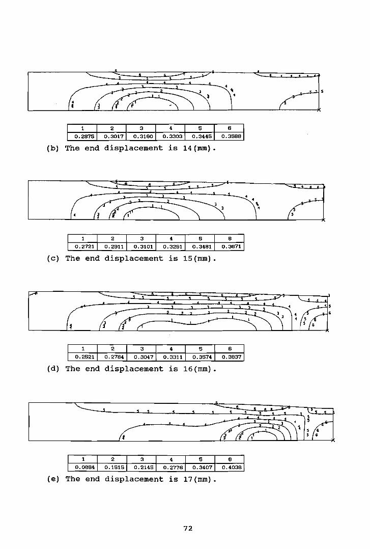
(b) The end displacement is 14(mm).

s

(c) The end displacement is 15(mm).

(d) The end displacement is 16(mm).

(e) The end displacement is 17(mm).

72

~ 5 5 5 5 5

:1(f) The end displacement is 18(mm).

c 5 5 5 5

(g) The end displacement is 19(mm).

(h) The end displacement is 20(mm).

Fig. B.2-3. The contour plots of triaxiality.

73